Design and Complex Dynamics of Potra–Pták-Type Optimal Methods for Solving Nonlinear Equations and Its Applications

Abstract

In this paper, using the idea of weight functions on the Potra–Pták method, an optimal fourth order method, a non optimal sixth order method, and a family of optimal eighth order methods are proposed. These methods are tested on some numerical examples, and the results are compared with some known methods of the corresponding order. It is proved that the results obtained from the proposed methods are compatible with other methods. The proposed methods are tested on some problems related to engineering and science. Furthermore, applying these methods on quadratic and cubic polynomials, their stability is analyzed by means of their basins of attraction.

1. Introduction

For solving nonlinear equations iteratively, the Newton’s method given by

$$x_{n+1}=x_n-\frac{f(x_n)}{f^{\prime }(x_n)}$$

is one of the most commonly used methods. The efficiency index as defined by Ostroswki in [1], which relates the order of convergence of a method p with the number of function evaluations per iteration d, is given by the expression $p^{1/d}$. Newton’s method is quadratically convergent and requires two function evaluations per iteration and, thereby, has the efficiency index value of $2^{1/2}\approx 1.414.$ Numerous methods have appeared giving higher order of convergence or better efficiency. One of the recent strategies to increase the order of the methods is the use of weight functions [2,3,4,5]. In this regard, Sharma and Behl [6] presented the fourth order method:

$$\begin{array}{cc}\hfill y_n& =x_n-\frac{2}{3}\frac{f(x_n)}{f^{\prime }(x_n)},\hfill \\ \hfill x_{n+1}& =x_n-\left(-\frac{1}{2}+\frac{3}{8}\frac{f^{\prime }(y_n)}{f^{\prime }(x_n)}+\frac{9}{8}\frac{f^{\prime }(x_n)}{f^{\prime }(y_n)}\right)\frac{f(x_n)}{f^{\prime }(x_n)}.\hfill \end{array}$$

(1)

Similarly, Sharifi et al. [7] used weight functions on the third order Heun’s method and proposed the fourth order method

$$\begin{array}{cc}\hfill y_n& =x_n-\frac{2}{3}\frac{f(x_n)}{f^{\prime }(x_n)},\hfill \\ \hfill x_{n+1}& =x_n-\frac{f(x_n)}{4}\left(\frac{1}{f^{\prime }(x_n)}+\frac{3}{f^{\prime }(y_n)}\right)\left(1+\frac{3}{8}{\left(\frac{f^{\prime }(y_n)}{f^{\prime }(x_n)}-1\right)}^2-\frac{69}{64}{\left(\frac{f^{\prime }(y_n)}{f^{\prime }(x_n)}-1\right)}^3+\frac{f(x_n)}{f^{\prime }(y_n)}\right).\hfill \end{array}$$

(2)

According to Kung and Traub [8], an iterative method is said to be optimal if its order is $2^{d-1},$ where d is the number of function evaluations per iteration. Notice that Newton’s method as well as (1) and (2) are all optimal.

Potra and Pták [9], as an attempt to improve Newton’s method, gave the method

$$\begin{array}{cc}\hfill y_n& =x_n-\frac{f(x_n)}{f^{\prime }(x_n)},\hfill \\ \hfill x_{n+1}& =x_n-\frac{f(x_n)+f(y_n)}{f^{\prime }(x_n)}.\hfill \end{array}$$

(3)

This method is cubically convergent but is not optimal, as it requires three function evaluations per iteration.

The aim, in the present paper, is to further investigate the method (3). Precisely, we use weight functions and improve the order of convergence of (3). We do it in three ways which correspond to the methods of orders 4, 6 and 8. Out of these, the methods with orders 4 and 8 are optimal.

Dynamics of a rational operator give important information about the convergence, efficiency and stability of the iterative methods. During the last few decades, many researchers, e.g., [10,11,12,13,14,15,16] and references therein, study the dynamical behavior of rational operators associated with iterative methods. Furthermore, there is an extensive literature [17,18,19,20,21] to understand and implement further results on the dynamics of rational functions. In this paper, we also analyze the dynamical behavior of the methods that we have developed in this paper. Furthermore, at the end of this work, the basins of attraction are also presented and compared among the proposed and other methods of the corresponding order.

The remaining part of the paper is organized as follows. In Section 2, the development of the methods and their convergence analysis are given. In Section 3, the proposed methods are tested on some functions, and the results are compared with other methods in the head of Numerical Examples. In Section 4, the proposed methods are tested on some engineering and science related designs. Section 5 is devoted to analyze the stability of the introduced methods by means of complex dynamics. In this sense, the study of the rational function resulting from the application of the methods to several nonlinear functions is developed, and their basins of attraction are represented. Finally, Section 6 covers the conclusions of the research.

2. Development of Methods and Their Convergence Analysis

In this section, the methods of order four, six and eight are introduced, and its convergence is analyzed.

2.1. Optimal Fourth Order Method

Based on the Potra–Pták method (3), we propose the following two-step method using a weight function, whose iterative expression is

$$\begin{array}{cc}\hfill y_n& =x_n-\frac{f\left(x_n\right)}{f^{\prime }\left(x_n\right)},\hfill \\ \hfill x_{n+1}& =x_n-w\left(t_n\right)\frac{f\left(x_n\right)+f\left(y_n\right)}{f^{\prime }\left(x_n\right)},\hfill \end{array}$$

(4)

where $w\left(t_n\right)=a_1+a_2{t}_n+a_3{t}_n^2$ and $t_n=\frac{f\left(y_n\right)}{f\left(x_n\right)}.$ The convergence of (4) is proved in the following theorem.

Theorem 1.

Let f be a real or complex valued function defined in the interval I having a sufficient number of smooth derivatives. Let α be a simple root of the equation $f\left(x\right)=0$ and the initial point $x_0$ is close enough to $\alpha .$ Then, the method (4) is fourth order of convergence if $a_1=1$, $a_2=0$ and $a_3=2$.

Proof. 

We denote $c_j=\frac{f^{\left(j\right)}\left(\alpha \right)}{j!f^{\prime }\left(\alpha \right)}.$ Let $e_n=x_n-\alpha$ be the error in $x_n.$ Then, Taylor’s series expansion of $f\left(x_n\right)$ and $f^{\prime }\left(x_n\right)$ about $\alpha$ gives

$$f\left(x_n\right)=f^{\prime }\left(\alpha \right)\left(e_n+c_2{e}_n^2+c_3{e}_n^3+c_4{e}_n^4+c_5{e}_n^5+c_6{e}_n^6+c_7{e}_n^7+c_8{e}_n^8+O\left(e_n^9\right)\right)$$

(5)

and

$$f^{\prime }\left(x_n\right)=f^{\prime }\left(\alpha \right)\left(1+2c_2{e}_n+3c_3{e}_n^2+4c_4{e}_n^3+5c_5{e}_n^4+6c_6{e}_n^5+7c_7{e}_n^6+8c_8{e}_n^7+O\left(e_n^8\right)\right).$$

(6)

Let $d_n=y_n-\alpha$, then, from the first equation of (4), we get

$$\begin{array}{cc}\hfill d_n=& c_2{e}_n^2-2\left(c_2^2-c_3\right)e_n^3+\left(4c_2^3-7c_2{c}_3+3c_4\right)e_n^4+\left(-8c_2^4+20c_3{c}_2^2-10c_4{c}_2-6c_3^2+4c_5\right)e_n^5\hfill \\ & +\left(16c_2^5-52c_3{c}_2^3+28c_4{c}_2^2+\left(33c_3^2-13c_5\right)c_2-17c_3{c}_4+5c_6\right)e_n^6\hfill \\ & -2\left(16c_2^6-64c_3{c}_2^4+36c_4{c}_2^3+9\left(7c_3^2-2c_5\right)c_2^2+\left(8c_6-46c_3{c}_4\right)c_2-9c_3^3+6c_4^2+11c_3{c}_5-3c_7\right)e_n^7\hfill \\ & +(64c_2^7-304c_3{c}_2^5+176c_4{c}_2^4+\left(408c_3^2-92c_5\right)c_2^3+\left(44c_6-348c_3{c}_4\right)c_2^2\hfill \\ & +75c_3^2{c}_4-31c_4{c}_5-27c_3{c}_6+c_2\left(-135c_3^3+118c_5{c}_3+64c_4^2-19c_7\right)+7c_8)e_n^8+O\left(e_n^9\right)\hfill \end{array}$$

so that, using Taylor’s series expansion of $f\left(y_n\right)$ about $\alpha$, we get

$$\begin{array}{cc}\hfill f\left(y_n\right)& =f(d_n+\alpha )\hfill \\ \hfill & =f^{\prime }\left(\alpha \right)[c_2{e}_n^2-2(c_2^2-c_3)e_n^3+\left(5c_2^3-7c_2{c}_3+3c_4\right)e_n^4-2\left(6c_2^4-12c_3{c}_2^2+5c_4{c}_2+3c_3^2-2c_5\right)e_n^5\hfill \\ \hfill & +\left(28c_2^5-73c_3{c}_2^3+34c_4{c}_2^2+\left(37c_3^2-13c_5\right)c_2-17c_3{c}_4+5c_6\right)e_n^6\hfill \\ \hfill & -2(32c_2^6-103c_3{c}_2^4+52c_4{c}_2^3+\left(80c_3^2-22c_5\right)c_2^2+\left(8c_6-52c_3{c}_4\right)c_2\hfill \\ \hfill & -9c_3^3+6c_4^2+11c_3{c}_5-3c_7)e_n^7+(144c_2^7-552c_3{c}_2^5+297c_4{c}_2^4+2\left(291c_3^2-67c_5\right)c_2^3\hfill \\ \hfill & +\left(54c_6-455c_3{c}_4\right)c_2^2+75c_3^2{c}_4-31c_4{c}_5-27c_3{c}_6+c_2\left(-147c_3^3+134c_5{c}_3+73c_4^2-19c_7\right)\hfill \\ \hfill & +7c_8)e_n^8+O\left(e_n^9\right)].\hfill \end{array}$$

(7)

Now, from (5) and (7), we get

$$\begin{array}{cc}\hfill t_n& =\frac{f\left(y_n\right)}{f\left(x_n\right)}\hfill \\ \hfill & =c_2{e}_n+(-3c_2^2+2c_3)e_n^2+(8c_2^3-10c_2{c}_3+3c_4)e_n^3+\left(-20c_2^4+37c_2^2{c}_3-14c_2{c}_4-8c_3^2+4c_5\right)e_n^4\hfill \\ \hfill & +\left(48c_2^5-118c_2^3{c}_3+51c_2^2{c}_4+55c_2{c}_3^2-18c_2{c}_5-22c_3{c}_4+5c_6\right)e_n^5\hfill \\ \hfill & +(-112c_2^6+344c_3{c}_2^4-163c_4{c}_2^3+\left(65c_5-252c_3^2\right)c_2^2+2\left(75c_3{c}_4-11c_6\right)c_2\hfill \\ \hfill & +26c_3^3-15c_4^2-28c_3{c}_5+6c_7)e_n^6+O\left(e_n^7\right).\hfill \end{array}$$

(8)

Therefore, using the results obtained above in the second equation of (4), we get

$$\begin{array}{cc}\hfill e_{n+1}& =\left(1-a_1\right)e_n-a_2{c}_2{e}_n^2+\left(2a_1{c}_2^2+3a_2{c}_2^2-2a_2{c}_3-a_3{c}_2^2\right)e_n^3\hfill \\ \hfill & +\left(-9a_1{c}_2^3+7a_1{c}_2{c}_3-6a_2{c}_2^3+10a_2{c}_2{c}_3-3a_2{c}_4+6a_3{c}_2^3-4a_3{c}_2{c}_3\right)e_n^4+O\left(e_n^5\right).\hfill \end{array}$$

(9)

In order to obtain fourth order of convergence, in view of (9), we must have

$$\begin{array}{cc}\hfill 1-a_1& =0,\hfill \\ \hfill a_2& =0,\hfill \\ \hfill 2a_1{c}_2^2+3a_2{c}_2^2-2a_2{c}_3-a_3{c}_2^2& =0,\hfill \end{array}$$

which gives $a_1=1$, $a_2=0$ and $a_3=2$. Therefore, from (9), the error equation of the method (4) becomes

$$e_{n+1}=(3c_2^3-c_2{c}_3)e_n^4+\mathcal{O}\left(e_n^5\right),$$

and the assertion follows. □

In view of Theorem 1, the proposed fourth order method is

$$\begin{array}{cc}\hfill y_n& =x_n-\frac{f\left(x_n\right)}{f^{\prime }\left(x_n\right)},\hfill \\ \hfill x_{n+1}& =x_n-\left(1+2{\left(\frac{f\left(y_n\right)}{f\left(x_n\right)}\right)}^2\right)\frac{f\left(x_n\right)+f\left(y_n\right)}{f^{\prime }\left(x_n\right)},\hfill \end{array}$$

(10)

which requires three function evaluations per iteration and consequently is optimal. In addition, the efficiency index of (10) is $1.5874$, which is higher than that of (3) having an efficiency index of $1.442$.

2.2. Sixth Order Method

Using the results obtained in (10), we propose a new method defined by

$$\begin{array}{cc}\hfill y_n& =x_n-\frac{f\left(x_n\right)}{f^{\prime }\left(x_n\right)},\hfill \\ \hfill z_n& =x_n-\left(1+2{\left(\frac{f\left(y_n\right)}{f\left(x_n\right)}\right)}^2\right)\frac{f\left(x_n\right)+f\left(y_n\right)}{f^{\prime }\left(x_n\right)},\hfill \\ \hfill x_{n+1}& =z_n-w_1\left(t_n\right)\frac{f\left(z_n\right)}{f^{\prime }\left(x_n\right)},\hfill \end{array}$$

(11)

where $w_1\left(t_n\right)=b_1+b_2{t}_n$ is a new weight function and $t_n$ is as in (4). The order of convergence is shown in the following result.

Theorem 2.

Let f be a real or complex valued function defined in an interval I having a sufficient number of smooth derivatives. Let α be a simple root of the equation $f\left(x\right)=0$ and the initial point $x_0$ is close enough to α. Then, (11) has a sixth order of convergence if $b_1=1$ and $b_2=2$.

Proof. 

Let ${\theta }_n=z_n-\alpha$. Then, from second equation of (11), we obtain

$$\begin{array}{cc}\hfill {\theta }_n& =(3c_2^3-c_2{c}_3)e_n^4-2\left(8c_2^4-10c_2^2{c}_3+c_3^2+c_2{c}_4\right)e_n^5\hfill \\ \hfill & +(46c_2^5-114c_2^3{c}_3+30c_2^2{c}_4+42c_2{c}_3^2-3c_2{c}_5-7c_3{c}_4)e_n^6+O\left(e_n^7\right).\hfill \end{array}$$

(12)

Now, by expanding $f\left(z_n\right)$ about $\alpha$ using Equation (12), we obtain

$$\begin{array}{cc}\hfill f\left(z_n\right)& =f({\theta }_n+\alpha )\hfill \\ \hfill & =f^{\prime }\left(\alpha \right)[\left(3c_2^3-c_2{c}_3\right)e_n^4-2\left(8c_2^4-10c_2^2{c}_3+c_3^2+c_2{c}_4\right)e_n^5\hfill \\ \hfill & +\left(46c_2^5-114c_2^3{c}_3+30c_2^2{c}_4+42c_2{c}_3^2-3c_2{c}_5-7c_3{c}_4\right)e_n^6+O\left(e_n^7\right)].\hfill \end{array}$$

(13)

Therefore, using (6), (8) and (13) in the third equation of (11), we obtain

$$\begin{array}{cc}\hfill e_{n+1}& =(1-b_1)c_2(3c_2^2-c_3)e_n^4\hfill \\ \hfill & +\left(c_2^4(22b_1-3b_2-16)+c_2^2{c}_3(-22b_1+b_2+20)+2(b_1-1)c_2{c}_4+2(b_1-1)c_3^2\right)e_n^5\hfill \\ \hfill & +(c_2^5(-90b_1+31b_2+46)+c_2^3{c}_3(167b_1-31b_2-114)+2c_2^2{c}_4(-17b_1+b_2+15)\hfill \\ \hfill & +c_2(c_3^2(-49b_1+4b_2+42)+3(b_1-1)c_5)+7(b_1-1)c_3{c}_4)e_n^6+O\left(e_n^7\right).\hfill \end{array}$$

(14)

In order to obtain sixth order of convergence, the coefficients of $e_n^4$ and $e_n^5$ must vanish in (14), i.e., $b_1=1$ and $b_2=2$. Therefore, the error equation of the method (11) becomes

$$e_{n+1}=c_2\left(18c_2^4-9c_2^2{c}_3+c_3^2\right)e_n^6+\mathcal{O}\left(e_n^7\right),$$

and the assertion follows. □

In view of Theorem 2, the following is the sixth order method

$$\begin{array}{cc}\hfill y_n& =x_n-\frac{f\left(x_n\right)}{f^{\prime }\left(x_n\right)},\hfill \\ \hfill z_n& =x_n-\left(1+2{\left(\frac{f\left(y_n\right)}{f\left(x_n\right)}\right)}^2\right)\frac{f\left(x_n\right)+f\left(y_n\right)}{f^{\prime }\left(x_n\right)},\hfill \\ \hfill x_{n+1}& =z_n-\left(1+2\frac{f\left(y_n\right)}{f\left(x_n\right)}\right)\frac{f\left(z_n\right)}{f^{\prime }\left(x_n\right)}.\hfill \end{array}$$

(15)

2.3. Optimal Eighth Order Method

Notice that the method (15) is not optimal as it requires four function evaluation per iteration to achieve sixth order of convergence. Its efficiency index is $1.5651$, which is less than that of the fourth order method (10). However, an eighth order method is obtained by (10) using an additional Newton step. The resulting iterative scheme is

$$\begin{array}{cc}\hfill y_n& =x_n-\frac{f\left(x_n\right)}{f^{\prime }\left(x_n\right)},\hfill \\ \hfill z_n& =x_n-\left(1+2{\left(\frac{f\left(y_n\right)}{f\left(x_n\right)}\right)}^2\right)\frac{f\left(x_n\right)+f\left(y_n\right)}{f^{\prime }\left(x_n\right)},\hfill \\ \hfill x_{n+1}& =z_n-\frac{f\left(z_n\right)}{f^{\prime }\left(z_n\right)}.\hfill \end{array}$$

(16)

Nevertheless, this method requires five function evaluation per iteration, so that its efficiency index reduces to $1.5157$, and, moreover, it is not optimal. Towards making the method (16) more efficient and optimal, we approximate $f^{\prime }\left(z\right)$ as

$$f^{\prime }\left(z_n\right)\approx \frac{f^{\prime }\left(x_n\right)}{J(t_n,u_n)·G\left(s_n\right)},$$

(17)

where

$$t_n=\frac{f\left(y_n\right)}{f\left(x_n\right)},u_n=\frac{f\left(z_n\right)}{f\left(x_n\right)},s_n=\frac{f\left(z_n\right)}{f\left(y_n\right)}.$$

Here, J and G are some appropriate weight functions of two variables and one variable, respectively. This type of approximations was done by Matthies et al. in [22]. Accordingly, we propose the following method:

$$\begin{array}{cc}\hfill y_n& =x_n-\frac{f\left(x_n\right)}{f^{\prime }\left(x_n\right)},\hfill \\ \hfill z_n& =x_n-\left(1+2{\left(\frac{f\left(y_n\right)}{f\left(x_n\right)}\right)}^2\right)\frac{f\left(x_n\right)+f\left(y_n\right)}{f^{\prime }\left(x_n\right)},\hfill \\ \hfill x_{n+1}& =z_n-\frac{f\left(z_n\right)}{f^{\prime }\left(x_n\right)}·J(t_n,u_n)·G\left(s_n\right),\hfill \end{array}$$

(18)

where $t_n,$ $u_n,$ and $s_n,$ are as in (17). For the method (18), we take the functions J and G as

$$J(t_n,u_n)=\frac{1+2t_n+(\beta +2)u_n+3t_n^2}{1+\beta u_n}$$

(19)

and

$$G\left(s_n\right)=\frac{1+\lambda s_n}{1+(\lambda -1)s_n},$$

(20)

where $\beta$ and $\lambda$ belong to $\mathbb{C}$. We prove the following result.

Theorem 3.

Let f be a real or complex valued function defined on some interval I having a sufficient number of smooth derivatives. Let α be a simple root of the equation $f\left(x\right)=0$ and the initial point $x_0$ is close enough to $\alpha .$ Then, (18) is an eighth order of convergence for the functions J and G given by (19) and (20), respectively.

Proof. 

In view of (5) and (13), we obtain

$$\begin{array}{cc}\hfill u_n& =\frac{f\left(z_n\right)}{f\left(x_n\right)}\hfill \\ & =\left(3c_2^3-c_2{c}_3\right)e_n^3+\left(-19c_2^4+21c_2^2{c}_3-2c_2{c}_4-2c_3^2\right)e_n^4\hfill \\ & +\left(65c_2^5-138c_2^3{c}_3+32c_2^2{c}_4+45c_2{c}_3^2-3c_2{c}_5-7c_3{c}_4\right)e_n^5+O\left(e_n^6\right).\hfill \end{array}$$

Similarly, (7) and (13) yield

$$\begin{array}{cc}\hfill s_n& =\frac{f\left(z_n\right)}{f\left(y_n\right)}\hfill \\ & =\left(3c_2^2-c_3\right)e_n^2-2\left(5c_2^3-6c_2{c}_3+c_4\right)e_n^3+\left(11c_2^4-44c_2^2{c}_3+17c_2{c}_4+11c_3^2-3c_5\right)e_n^4\hfill \\ & +\left(56c_2^5+28c_2^3{c}_3-56c_2^2{c}_4-60c_2{c}_3^2+22c_2{c}_5+30c_3{c}_4-4c_6\right)e_n^5+O\left(e_n^6\right).\hfill \end{array}$$

Consequently, (19) gives

$$\begin{array}{cc}\hfill J(t_n,u_n)& =1+2c_2{e}_n+\left(4c_3-3c_2^2\right)e_n^2+\left(4c_2^3-10c_2{c}_3+6c_4\right)e_n^3\hfill \\ \hfill & +\left(-3(2\beta +1)c_2^4+2(\beta +10)c_2^2{c}_3-14c_2{c}_4-8c_3^2+8c_5\right)e_n^4\hfill \\ \hfill & +((47\beta -38)c_2^5-(57\beta +14)c_2^3{c}_3+4(\beta +7)c_2^2{c}_4\hfill \\ \hfill & +2c_2\left(4(\beta +4)c_3^2-9c_5\right)-22c_3{c}_4+10c_6)e_n^5+O\left(e_n^6\right),\hfill \end{array}$$

(21)

and (20) gives

$$\begin{array}{cc}\hfill G\left(s_n\right)& =1+\left(3c_2^2-c_3\right)e_n^2-2\left(5c_2^3-6c_2{c}_3+c_4\right)e_n^3\hfill \\ \hfill & +\left((20-9\lambda )c_2^4+2(3\lambda -25)c_2^2{c}_3-(\lambda -12)c_3^2+17c_2{c}_4-3c_5\right)e_n^4\hfill \\ \hfill & +2((30\lambda -2)c_2^5+(60-46\lambda )c_2^3{c}_3+2(3\lambda -17)c_2^2{c}_4+c_2\left(6(2\lambda -7)c_3^2+11c_5\right)\hfill \\ \hfill & +(17-2\lambda )c_3{c}_4-2c_6)e_n^5+O\left(e_n^6\right).\hfill \end{array}$$

(22)

Now, using the values from (6), (12), (13), (21), and (22) in (18), the error equation of the method is

$$e_{n+1}=c_2\left(3c_2^2-c_3\right)\left(c_2^4(6\beta +9\lambda +9)-2c_2^2{c}_3(\beta +3\lambda +4)+c_2{c}_4+c_3^2\lambda \right)e_n^8+\mathcal{O}\left(e_n^9\right),$$

which gives the eighth order of convergence. □

3. Numerical Examples

In this section, we test the performance of the methods proposed in Section 2 with the help of some numerical examples. We compare the results obtained with the known methods of the corresponding order. We consider the following nonlinear equations and initial guesses:

• $f_1\left(x\right)={sin}^{2}x-x^2+1,x_0=2,$
• $f_2\left(x\right)=ln(1+x^2)+exp(x^2-3x)sinx,x_0=2,$
• $f_3\left(x\right)=x^2-{(1-x)}^5,x_0=1,$
• $f_4\left(x\right)=x^2-exp\left(x\right)-3x+2,x_0=1,$
• $f_5\left(x\right)=\sqrt{x^2+2x+5}-2sinx-x^2+3,x_0=2.$

In the previous section, we have proved the theoretical order of convergence of various methods. For practical purposes, we can test numerically the order of convergence of these methods by using Approximated Computational Order of Convergence (or ACOC), defined by Cordero and Torregrosa [23]. They defined the ACOC of a sequence $\left\{x_k\right\},k\ge 0$ as

$$ACOC=\frac{log\left(\left|x_{k+1}-x_k\right|/\left|x_k-x_{k-1}\right|\right)}{log\left(\left|x_k-x_{k-1}\right|/\left|x_{k-1}-x_{k-2}\right|\right)}.$$

(23)

The use of $ACOC$, given by (23), serves as a practical check on the theoretical error calculations.

We apply our proposed methods and other existing methods as discussed in the following subsections on each of the test functions. Various results of up to four iterations are observed, and we compare the results obtained at the 4th iteration among different methods of the corresponding order and shown in

Table 1. Comparison of numerical results of fourth order methods at the 4th iteration.

		${\mathit{f}}_1$	${\mathit{f}}_2$	${\mathit{f}}_3$	${\mathit{f}}_4$	${\mathit{f}}_5$
$\Delta x_n$	$M_{41}$	8.7309 × 10${}^{-26}$	2.7730 × 10${}^{-55}$	9.9454 × 10${}^{-30}$	1.2399 × 10${}^{-65}$	9.2139 × 10${}^{-82}$
	$M_{42}$	1.1188 × 10${}^{-27}$	2.9815 × 10${}^{-28}$	1.0915 × 10${}^{-24}$	7.7434 × 10${}^{-72}$	3.5851 × 10${}^{-101}$
	$M_{43}$	1.1523 × 10${}^{-23}$	NC	6.1887 × 10${}^{-13}$	1.3049 × 10${}^{-15}$	3.6376 × 10${}^{-49}$
	$M_{44}$	2.0493 × 10${}^{-32}$	2.0594 × 10${}^{-31}$	1.1971 × 10${}^{-20}$	1.5448 × 10${}^{-71}$	1.1488 × 10${}^{-97}$
	$M_{45}$	4.0043 × 10${}^{-28}$	2.8464 × 10${}^{-57}$	2.4018 × 10${}^{-30}$	4.7295 × 10${}^{-65}$	2.8215 × 10${}^{-81}$
$x_n$	$M_{41}$	1.4045	−7.8835 × 10${}^{-218}$	0.3460	0.2575	2.3320
	$M_{42}$	1.4045	−6.9805 × 10${}^{-110}$	0.3460	0.2575	2.3320
	$M_{43}$	1.4045	NC	0.3460	0.2575	2.3320
	$M_{44}$	1.4045	3.2977 × 10${}^{-123}$	0.3460	0.2575	2.3320
	$M_{45}$	1.4045	−3.5010 × 10${}^{-226}$	0.3460	0.2575	2.3320
$\left|f\right(x_n\left)\right|$	$M_{41}$	1.9828 × 10${}^{-100}$	7.8835 × 10${}^{-218}$	1.9230 × 10${}^{-116}$	2.5756 × 10${}^{-262}$	1.1861 × 10${}^{-326}$
	$M_{42}$	4.0436 × 10${}^{-108}$	6.9805 × 10${}^{-110}$	1.1758 × 10${}^{-96}$	6.8107 × 10${}^{-287}$	1.9034 × 10${}^{-404}$
	$M_{43}$	3.6237 × 10${}^{-93}$	NC	6.4877 × 10${}^{-49}$	7.5782 × 10${}^{-62}$	2.9990 × 10${}^{-196}$
	$M_{44}$	1.7439 × 10${}^{-127}$	3.2977 × 10${}^{-123}$	4.4608 × 10${}^{-80}$	1.3131 × 10${}^{-285}$	2.5652 × 10${}^{-390}$
	$M_{45}$	5.7027 × 10${}^{-110}$	3.5010 × 10${}^{-226}$	9.4841 × 10${}^{-120}$	6.9959 × 10${}^{-260}$	1.1952 × 10${}^{-324}$
$ACOC$	$M_{41}$	3.9919	4.0000	4.0184	4.0000	4.0000
	$M_{42}$	3.9935	3.9953	4.0646	4.0000	4.0000
	$M_{43}$	4.1336	NC	3.5972	4.6265	4.0214
	$M_{44}$	3.9978	4.0069	3.9838	4.0000	4.0000
	$M_{45}$	3.9946	4.0001	3.9878	4.0000	4.0000

,

Table 2. Comparison of numerical results of sixth order methods at the 4th iteration.

		${\mathit{f}}_1$	${\mathit{f}}_2$	${\mathit{f}}_3$	${\mathit{f}}_4$	${\mathit{f}}_5$
$\Delta x_n$	$M_{61}$	1.8933 × 10${}^{-73}$	1.8896 × 10${}^{-148}$	5.1627 × 10${}^{-90}$	1.3377 × 10${}^{-199}$	9.5891 × 10${}^{-261}$
	$M_{62}$	1.6801 × 10${}^{-106}$	2.9382 × 10${}^{-152}$	2.4137 × 10${}^{-64}$	1.7893 × 10${}^{-191}$	3.75383 × 10${}^{-255}$
	$M_{63}$	2.9803 × 10${}^{-95}$	2.9803 × 10${}^{-95}$	2.9815 × 10${}^{-82}$	2.9815 × 10${}^{-82}$	2.9803 × 10${}^{-95}$
	$M_{64}$	5.0012 × 10${}^{-85}$	2.4246 × 10${}^{-153}$	4.9788 × 10${}^{-69}$	4.6397 × 10${}^{-198}$	4.0268 × 10${}^{-259}$
	$M_{65}$	9.9516 × 10${}^{-88}$	2.1737 × 10${}^{-154}$	3.3993 × 10${}^{-86}$	2.7764 × 10${}^{-193}$	3.4903 × 10${}^{-256}$
$x_n$	$M_{61}$	1.4045	−1.1331 × 10${}^{-884}$	0.3460	0.2575	2.3320
	$M_{62}$	1.4045	4.5753 × 10${}^{-908}$	0.3460	0.2575	2.3320
	$M_{63}$	1.4045	1.4045	0.3460	0.2575	1.4045
	$M_{64}$	1.4045	1.0114 × 10${}^{-914}$	0.3460	0.2575	2.3320
	$M_{65}$	1.4045	−3.7511 × 10${}^{-921}$	0.3460	0.2575	2.3320
$\left|f\right(x_n\left)\right|$	$M_{61}$	5.6523 × 10${}^{-436}$	1.1331 × 10${}^{-884}$	1.8046 × 10${}^{-535}$	0.0	0.0
	$M_{62}$	6.7308 × 10${}^{-636}$	4.5753 × 10${}^{-908}$	1.0347 × 10${}^{-381}$	0.0	0.0
	$M_{63}$	8.1802 × 10${}^{-568}$	8.1802 × 10${}^{-568}$	8.2004 × 10${}^{-490}$	8.2004 × 10${}^{-490}$	8.1802 × 10${}^{-568}$
	$M_{64}$	5.7605 × 10${}^{-506}$	1.0114 × 10${}^{-914}$	1.8726 × 10${}^{-409}$	0.0	0.0
	$M_{65}$	3.7794 × 10${}^{-522}$	3.7511 × 10${}^{-921}$	4.8072 × 10${}^{-514}$	0.0	0.0
$ACOC$	$M_{61}$	5.9980	6.0000	5.9980	6.0000	6.0000
	$M_{62}$	5.9992	6.0000	5.9854	6.0000	6.000
	$M_{63}$	5.9997	5.9997	5.9992	5.9992	5.9997
	$M_{64}$	5.9991	6.0000	5.9984	6.0000	6.0000
	$M_{65}$	5.9993	6.0000	6.0088	6.0000	6.0000

and

Table 3. Comparison of numerical results of eighth order methods at the 4th iteration.

		${\mathit{f}}_1$	${\mathit{f}}_2$	${\mathit{f}}_3$	${\mathit{f}}_4$	${\mathit{f}}_5$
$\Delta x_n$	$M_{81}$	5.8768 × 10${}^{-187}$	1.5404 × 10${}^{-393}$	2.5345 × 10${}^{-165}$	6.1099 × 10${}^{-495}$	4.4344 × 10${}^{-658}$
	$M_{82}$	2.0563 × 10${}^{-165}$	9.0158 × 10${}^{-321}$	1.1101 × 10${}^{-167}$	5.4494 × 10${}^{-421}$	4.0437 × 10${}^{-598}$
	$M_{83}$	4.5429 × 10${}^{-170}$	1.5139 × 10${}^{-324}$	2.9710 × 10${}^{-168}$	2.8838 × 10${}^{-421}$	2.9107 × 10${}^{-604}$
	$M_{84}$	2.4469 × 10${}^{-187}$	4.9438 × 10${}^{-351}$	4.3825 × 10${}^{-171}$	1.8592 × 10${}^{-438}$	4.3404 × 10${}^{-614}$
	$M_{85}$	2.6744 × 10${}^{-204}$	NC	1.7766 × 10${}^{-177}$	6.5231 × 10${}^{-192}$	9.8976 × 10${}^{-553}$
	$M_{86}$	4.1482 × 10${}^{-235}$	1.3271 × 10${}^{-380}$	5.6991 × 10${}^{-175}$	2.5934 × 10${}^{-455}$	7.1011 × 10${}^{-617}$
$x_n$	$M_{81}$	1.4045	0.0	0.3460	0.2575	2.3320
	$M_{82}$	1.4045	0.0	0.3460	0.2575	2.3320
	$M_{83}$	1.4045	0.0	0.3460	0.2575	2.3320
	$M_{84}$	1.4045	0.0	0.3460	0.2575	2.3320
	$M_{85}$	1.4045	NC	0.3460	0.2575	2.3320
	$M_{86}$	1.4045	0.0	0.3460	0.2575	2.3320
$\left|f\right(x_n\left)\right|$	$M_{81}$	0.0	0.0	0.0	0.0	0.0
	$M_{82}$	0.0	0.0	0.0	0.0	0.0
	$M_{83}$	0.0	0.0	0.0	0.0	0.0
	$M_{84}$	0.0	0.0	0.0	0.0	0.0
	$M_{85}$	0.0	0.0	0.0	0.0	0.0
	$M_{86}$	0.0	0.0	0.0	0.0	0.0
$ACOC$	$M_{81}$	7.9999	8.0000	7.9993	8.0000	8.0000
	$M_{82}$	7.9996	8.0000	8.0000	8.0000	8.0000
	$M_{83}$	7.9997	8.0000	7.9996	8.0000	8.0000
	$M_{84}$	7.9998	8.0000	8.0047	8.0000	8.0000
	$M_{85}$	7.9995	NC	8.0020	8.0004	8.0000
	$M_{86}$	8.0000	8.0000	8.0023	8.0000	8.0000

. For a particular test function, we take the same initial guess $x_0$ for each of the methods under consideration. We compare the approximate error $\Delta x_n\equiv |x_n-x_{n-1}|,$ the approximate solution $x_n,$ the absolute value of corresponding functional value $\left|f\right(x_n\left)\right|$, and approximated computational order of convergence $\left(ACOC\right)$ at $n=4.$ In the tables, “NC” stands for no convergence of the method. We use Mathematica $9.0$ for the calculations.

3.1. Comparison of the Fourth Order Method

Let us denote our method (10) by $M_{41}.$ We shall compare this method with

• Sharma and Behl method (1), denoted by $M_{42}$,
• Sharifi et al. method (2), denoted by $M_{43}$,
• Jarratt’s method [24], denoted by $M_{44}$ and given by

  $$\begin{array}{cc}\hfill y_n& =x_n-\frac{2}{3}\frac{f\left(x_n\right)}{f^{\prime }\left(x_n\right)},\hfill \\ \hfill x_{n+1}& =x_n-\left(\frac{3f^{\prime }\left(y_n\right)+f^{\prime }\left(x_n\right)}{6f^{\prime }\left(y_n\right)-2f^{\prime }\left(x_n\right)}\right)\frac{f\left(x_n\right)}{f^{\prime }\left(x_n\right)},\hfill \end{array}$$
• Kung–Traub [8] method, denoted by $M_{45}$, and given by

  $$\begin{array}{cc}\hfill y_n& =x_n-\frac{f\left(x_n\right)}{f^{\prime }\left(x_n\right)},\hfill \\ \hfill x_{n+1}& =y_n-\left(\frac{f\left(x_n\right)·f\left(y_n\right)}{{(f\left(x_n\right)-f\left(y_n\right))}^2}\right)\frac{f\left(x_n\right)}{f^{\prime }\left(x_n\right)}.\hfill \end{array}$$

All the methods $M_{4i},$ $i=1,2,3,4,5$ are optimal. Table 1 records the performance of all these methods.

3.2. Comparison of Sixth Order Methods

We denote our sixth order method (15) by $M_{61}.$ We shall compare this method with

• $M_{62}:$ Method of Neta [25] with $a=1$, given by

  $$\begin{array}{cc}\hfill y_n& =x_n-\frac{f\left(x_n\right)}{f^{\prime }\left(x_n\right)},\hfill \\ \hfill z_n& =y_n-\frac{f\left(x_n\right)+af\left(y_n\right)}{f\left(x_n\right)+(a-2)f\left(y_n\right)}\frac{f\left(y_n\right)}{f^{\prime }\left(x_n\right)},\hfill \\ \hfill x_{n+1}& =z_n-\frac{f\left(x_n\right)-f\left(y_n\right)}{f\left(x_n\right)-3f\left(y_n\right)}\frac{f\left(z_n\right)}{f^{\prime }\left(x_n\right)},\hfill \end{array}$$
• $M_{63}:$ Method of Grau et al. [26] given by

  $$\begin{array}{cc}\hfill y_n& =x_n-\frac{f\left(x_n\right)}{f^{\prime }\left(x_n\right)},\hfill \\ \hfill z_n& =y_n-\frac{f\left(y_n\right)}{f^{\prime }\left(x_n\right)}\frac{f\left(x_n\right)}{f\left(x_n\right)-2f\left(y_n\right)},\hfill \\ \hfill x_{n+1}& =z_n-\frac{f\left(z_n\right)}{f^{\prime }\left(x_n\right)}\frac{f\left(x_n\right)}{f\left(x_n\right)-2f\left(y_n\right)}.\hfill \end{array}$$
• $M_{64}:$ Method of Sharma and Guha [27] with $a=2$, given by

  $$\begin{array}{cc}\hfill y_n& =x_n-\frac{f\left(x_n\right)}{f^{\prime }\left(x_n\right)},\hfill \\ \hfill z_n& =y_n-\frac{f\left(y_n\right)}{f^{\prime }\left(x_n\right)}\frac{f\left(x_n\right)}{f\left(x_n\right)-2f\left(y_n\right)},\hfill \\ \hfill x_{n+1}& =z_n-\frac{f\left(z_n\right)}{f^{\prime }\left(x_n\right)}\frac{f\left(x_n\right)+af\left(y_n\right)}{f\left(x_n\right)+(a-2)f\left(y_n\right)},\hfill \end{array}$$
• $M_{65}:$ Method of Chun and Neta [28] given by

  $$\begin{array}{cc}\hfill y_n& =x_n-\frac{f\left(x_n\right)}{f^{\prime }\left(x_n\right)},\hfill \\ \hfill z_n& =y_n-\frac{f\left(y_n\right)}{f^{\prime }\left(x_n\right)}\frac{1}{{\left(1-\frac{f\left(y_n\right)}{f\left(x_n\right)}\right)}^2},\hfill \\ \hfill x_{n+1}& =z_n-\frac{f\left(y_n\right)}{f^{\prime }\left(x_n\right)}\frac{1}{{\left(1-\frac{f\left(y_n\right)}{f\left(x_n\right)}-\frac{f\left(z_n\right)}{f\left(x_n\right)}\right)}^2}.\hfill \end{array}$$

The comparison of the methods $M_{6i},$ $i=1,2,3,4,5$ is tabulated in Table 2. From the table, we observe that the proposed method $M_{61}$ is compatible with the other existing methods. We can see that method $M_{63}$ gives different results for the test functions $f_2$ and $f_5$ with given initial guesses.

3.3. Comparison of Eighth Order Methods

Consider the eighth order method (18), which involves the parameter pair $(\beta ,\lambda ).$ We denote

• $M_{81}$ the case where $(\beta ,\lambda )=(0,0)$, whose iterative expression results in

  $$\begin{array}{cc}\hfill y_n& =x_n-\frac{f\left(x_n\right)}{f^{\prime }\left(x_n\right)},\hfill \\ \hfill z_n& =x_n-\frac{f\left(x_n\right)+f\left(y_n\right)}{f^{\prime }\left(x_n\right)}\left(1+2{\left(\frac{f\left(y_n\right)}{f\left(x_n\right)}\right)}^2\right),\hfill \\ \hfill x_{n+1}& =z_n-\frac{f\left(z_n\right)}{f^{\prime }\left(x_n\right)}\left(\frac{1+2t_n+2u_n+3t_n^2}{1-s_n}\right),\hfill \end{array}$$
• $M_{82}$ for $(\beta ,\lambda )=(1,1)$, resulting in the iterative scheme given by $M_{81}:$

  $$\begin{array}{cc}\hfill y_n& =x_n-\frac{f\left(x_n\right)}{f^{\prime }\left(x_n\right)},\hfill \\ \hfill z_n& =x_n-\frac{f\left(x_n\right)+f\left(y_n\right)}{f^{\prime }\left(x_n\right)}\left(1+2{\left(\frac{f\left(y_n\right)}{f\left(x_n\right)}\right)}^2\right),\hfill \\ \hfill x_{n+1}& =z_n-\frac{f\left(z_n\right)}{f^{\prime }\left(x_n\right)}\left(\frac{1+2t_n+3u_n+3t_n^2}{1+u_n}(1+s_n)\right),\hfill \end{array}$$
• $M_{83}$ for $(\beta ,\lambda )=(0,1)$, whose iterative method is

  $$\begin{array}{cc}\hfill y_n& =x_n-\frac{f\left(x_n\right)}{f^{\prime }\left(x_n\right)},\hfill \\ \hfill z_n& =x_n-\frac{f\left(x_n\right)+f\left(y_n\right)}{f^{\prime }\left(x_n\right)}\left(1+2{\left(\frac{f\left(y_n\right)}{f\left(x_n\right)}\right)}^2\right),\hfill \\ \hfill x_{n+1}& =z_n-\frac{f\left(z_n\right)}{f^{\prime }\left(x_n\right)}\left((1+2t_n+2u_n+3t_n^2)(1+s_n)\right).\hfill \end{array}$$

Along with these, we take the following methods for the comparison of numerical results:

• Matthies et al. in [22] presented an optimal class of $8th$ order method from the Kung–Traub method [8]. For some particular values of the parameters, one of the methods denoted by $M_{84}$ is given by

  $$\begin{array}{cc}\hfill y_n& =x_n-\frac{f\left(x_n\right)}{f^{\prime }\left(x_n\right)},\hfill \\ \hfill z_n& =y_n-\left(\frac{f\left(x_n\right)f\left(y_n\right)}{{(f\left(x_n\right)-f\left(y_n\right))}^2}\right)\frac{f\left(x_n\right)}{f^{\prime }\left(x_n\right)},\hfill \\ \hfill x_{n+1}& =z_n-\frac{f\left(z_n\right)}{f^{\prime }\left(x_n\right)}\left(\frac{2+t_n+5u_n+4t_n^2+4t_n^3}{2-3t_n+u_n+2t_n^2}·\frac{2+s_n}{2-s_n}\right).\hfill \end{array}$$
• Babajee et al. in [11] presented a family of eighth order methods. For some fixed values of parameters, the method denoted by $M_{85}$ is given by

  $$\begin{array}{cc}\hfill y_n& =x_n-\frac{f\left(x_n\right)}{f^{\prime }\left(x_n\right)}\left(1+{\left(\frac{f\left(x_n\right)}{f^{\prime }\left(x_n\right)}\right)}^5\right),\hfill \\ \hfill z_n& =y_n-\frac{f\left(y_n\right)}{f^{\prime }\left(x_n\right)}{\left(1-\frac{f\left(y_n\right)}{f\left(x_n\right)}\right)}^{-2},\hfill \\ \hfill x_{n+1}& =z_n-\frac{f\left(z_n\right)}{f^{\prime }\left(x_n\right)}\left(\frac{(1+t_n^2+5t_n^4+s_n}{{\left(1-t_n-u_n\right)}^2}\right).\hfill \end{array}$$
• Chun and Lee in [29] presented a family of optimal eighth order methods. For some particular values of parameters, the method denoted by $M_{86}$ is given by

  $$\begin{array}{cc}\hfill y_n& =x_n-\frac{f\left(x_n\right)}{f^{\prime }\left(x_n\right)},\hfill \\ \hfill z_n& =y_n-\frac{f\left(y_n\right)}{f^{\prime }\left(x_n\right)}\frac{1}{{\left(1-\frac{f\left(y_n\right)}{f\left(x_n\right)}\right)}^2},\hfill \\ \hfill x_{n+1}& =z_n-\frac{f\left(z_n\right)}{f^{\prime }\left(x_n\right)}\frac{1}{{\left(1-t_n-\frac{t_n^2}{2}+\frac{t_n^3}{2}-\frac{u_n}{2}-\frac{s_n}{2}\right)}^2}.\hfill \end{array}$$

In all the above methods, $t_n$, $u_n$ and $s_n$ are as given in (17). The performance of the methods $M_{8i},$ $i=1,2,3,4,5,6$ are recorded in Table 3.

From Table 1, Table 2 and Table 3, we observe that the proposed methods are compatible with other existing methods (and sometimes perform better than other methods) of the corresponding order. Not any particular method is superior to others for all examples. Among the family of eighth order methods (18), from Table 3, we observe that the method $M_{81}$ performs better than other two. For more understanding about the iterative methods, we study the dynamics of these methods in the next section.

4. Applications

The applications discussed in Section 4.1, Section 4.2 and Section 4.3 are based on standard engineering examples, and we refer to [30]. We use the proposed methods $M_{41},$ $M_{61},$ and $M_{8i},$ $i=1,2,3$ to obtain the various results from the first three iterations of these examples. In particular, we compute the value of the unknowns $x_{n-1}$ and $x_n$, absolute value of the function $f\left(x_n\right)$ and absolute value of the difference d of unknown in two consecutive iterations, i.e., $d=|x_n-x_{n-1}|,$$n=1,2,3.$

4.1. Pipe Friction Problem

Determining fluid flow through pipes and tubes has great relevance in many areas of engineering and science. In engineering, typical applications include the flow of liquids and gases through pipelines and cooling systems. Scientists are interested in topics ranging from flow in blood vessels to nutrient transmission through a plant’s vascular system. The resistance to flow in such conduits is parameterized by a dimensionless number called the friction factor $f.$ For a flow with turbulence, the Colebrook equation [31] provides a means to calculate the friction factor:

$$0=\frac{1}{\sqrt{f}}+2.0log\left(\frac{ϵ}{3.7D}+\frac{2.51}{Re\sqrt{f}}\right),$$

(24)

where $ϵ$ is the roughness (m), D is the diameter (m) and $Re$ is the Reynolds number

$$Re=\frac{\rho vD}{\mu }.$$

Here, $\rho$ denotes the fluid density (kg/m${}^3$), v the velocity of the fluid (m/s) and $\mu$ the dynamical viscosity (N·s/m${}^2$). A flow is said to be turbulent if $Re>4000.$

To determine f for air flow through a smooth and thin tube, the parameters are taken to be $\rho$ = 1.23 kg/m${}^3$, $\mu =1.79\times {10}^{-5}$ N·s/m${}^2$, $D=0.005$ m, $V=40$ m/s and $ϵ=0.0000015$ m. Since the friction factors range from about 0.008 to 0.08, we choose initial guess $f_0=0.023.$ To determine the approximate value of $f$, we use the function

$$g\left(f\right)=\frac{1}{\sqrt{f}}+2.0log\left(\frac{ϵ}{3.7D}+\frac{2.51}{Re\sqrt{f}}\right).$$

(25)

The results obtained by the various methods are presented in

Table 4. Results of pipe friction problem.

# Iter	Value	${\mathit{M}}_{41}$	${\mathit{M}}_{61}$	${\mathit{M}}_{81}$	${\mathit{M}}_{82}$	${\mathit{M}}_{83}$
1	f	0.0169	0.0170	0.0170	0.0170	0.0170
	$g\left(f\right)$	0.0240	0.0104	0.0009	0.0005	0.0008
	d	0.0061	0.0060	0.0060	0.0060	0.0060
2	f	0.0170	0.0170	0.0170	0.0170	0.0170
	$g\left(f\right)$	3.0954 × 10${}^{-9}$	2.6645 × 10${}^{-15}$	8.8818 × 10${}^{-16}$	8.8818 × 10${}^{-16}$	8.8818 × 10${}^{-16}$
	d	0.0001	4.1700 × 10${}^{-5}$	3.7223 × 10${}^{-6}$	2.0962 × 10${}^{-6}$	3.3172 × 10${}^{-6}$
3	f	0.0170	0.0170	0.0170	0.0170	0.0170
	$g\left(f\right)$	8.8818 × 10${}^{-16}$	8.8818 × 10${}^{-16}$	8.8818 × 10${}^{-16}$	8.8818 × 10${}^{-16}$	8.8818 × 10${}^{-16}$
	d	1.2442 × 10${}^{-11}$	1.0408 × 10${}^{-17}$	6.9389 × 10${}^{-18}$	0.0	0.0

.

4.2. Open-Channel Flow

An open problem in civil engineering is to relate the flow of water with other factors affecting the flow in open channels such as rivers or canals. The flow rate is determined as the volume of water passing a particular point in a channel per unit time. A further concern is related to what happens when the channel is slopping.

Under uniform flow conditions, the flow of water in an open channel is given by Manning’s equation

$$Q=\frac{\sqrt{S}}{n}A{R}^{2/3},$$

(26)

where S is the slope of the channel, A is the cross-sectional area of the channel, R is the hydraulic radius of the channel and n is the Manning’s roughness coefficient. For a rectangular channel having the width B and the defth of water in the channel $y,$ it is known that

$$A=By$$

and

$$R=\frac{By}{B+2y}.$$

With these values, (26) becomes

$$Q=\frac{\sqrt{S}}{n}By{\left(\frac{By}{B+2y}\right)}^{2/3}.$$

(27)

Now, if it is required to determine the depth of water in the channel for a given quantity of water, (27) can be rearranged as

$$f\left(y\right)=\frac{\sqrt{S}}{n}By{\left(\frac{By}{B+2y}\right)}^{2/3}-Q.$$

(28)

In our work, we estimate y when the remaining parameters are assumed to be given as $Q=14.15$ m${}^3$/s, $B=4.572$ m, $n=0.017$ and $S=0.0015.$ We choose as an initial guess $y_0=4.5$ m. The results obtained by the various methods are presented in

Table 5. Results of an open channel problem.

# Iter	Value	${\mathit{M}}_{41}$	${\mathit{M}}_{61}$	${\mathit{M}}_{81}$	${\mathit{M}}_{82}$	${\mathit{M}}_{83}$
1	y	1.4804	1.4666	1.4652	1.4653	1.4653
	$f\left(y\right)$	0.2088	0.0204	0.0016	0.0029	0.0028
	d	3.0200	3.0334	3.0348	3.0347	3.0347
2	y	1.4651	1.4651	1.4651	1.4651	1.4651
	$f\left(y\right)$	4.5027 × 10${}^{-9}$	1.7764 × 10${}^{-15}$	× 10${}^{-15}$	3.5527 × 10${}^{-15}$	3.5527 × 10${}^{-15}$
	d	0.0154	0.0015	0.0001	0.0002	0.0002
3	y	1.4651	1.4651	1.4651	1.4651	1.4651
	$f\left(y\right)$	3.5527 × 10${}^{-15}$	7.1054 × 10${}^{-14}$	6.5725 × 10${}^{-14}$	5.3291 × 10${}^{-15}$	1.7764 × 10${}^{-15}$
	d	3.3152 × 10${}^{-10}$	5.1070 × 10${}^{-15}$	5.1070 × 10${}^{-15}$	6.6613 × 10${}^{-16}$	2.2204 × 10${}^{-16}$

.

4.3. Ideal and Non-Ideal Gas Laws

The ideal gas law is

$$PV=nRT,$$

where P is the absolute pressure, V is the volume, n is the number of moles, R is the universal gas constant and T is the absolute temperature. Due to its limited use in engineering, an alternative equation of state for gases is the given van der Waals equation [32,33,34,35]

$$\left(P+\frac{a}{v^2}\right)(v-b)=RT,$$

where $v=\frac{V}{n}$ is the molal volume and $a,b$ are empirical constants that depend on the particular gas. The computation of the molal volume is done by solving

$$f\left(v\right)=\left(P+\frac{a}{v^2}\right)(v-b)-RT.$$

(29)

We take the remaining parameters as $R=0.082054$ L atm/(mol K), for carbon dioxide $a=3.592,$$b=0.04267,$ $T=300$ K, $p=1$ atm, and the initial guess for the molal volume is taken as $v_0=3.$ The results obtained by the various methods are presented in

Table 6. Numerical results of ideal and non-ideal gas law.

# Iter	Value	${\mathit{M}}_{41}$	${\mathit{M}}_{61}$	${\mathit{M}}_{81}$	${\mathit{M}}_{82}$	${\mathit{M}}_{83}$
1	v	26.4881	27.0049	23.9583	24.1631	24.0274
	$f\left(v\right)$	1.9647	2.4788	0.5509	0.3474	0.4823
	d	23.4881	24.0049	20.9583	21.1631	21.0274
2	v	24.5126	24.5126	24.5126	24.5126	24.5126
	$f\left(v\right)$	2.7340 × 10${}^{-8}$	3.3573 × 10${}^{-12}$	0.0	0.0	0.0
	d	1.9756	2.4923	0.5543	0.3495	0.4852
3	v	24.5126	24.5126	$IND$	$IND$	$IND$
	$f\left(v\right)$	0.0	0.0	$IND$	$IND$	$IND$
	d	2.7503 × 10${}^{-8}$	3.3786 × 10${}^{-12}$	$IND$	$IND$	$IND$

. In this table, $IND$ stands for indeterminate form.

5. Dynamical Analysis

The stability analysis of the methods $M_{41}$, $M_{61}$ and $M_{8i}$, $i=1,2,3$, is performed in this section. The dynamics of the proposed methods on a generic quadratic polynomial will be studied, analyzing the associated rational operator for each method. This analysis shows their performance depending on the initial estimations. In addition, method $M_{41}$ is analyzed for cubic polynomials. First, we recall some basics on complex dynamics.

5.1. Basics on Complex Dynamics

Let $R:\widehat{\mathbb{C}}⟶\widehat{\mathbb{C}}$ be a rational function defined on the Riemann sphere. Let us recall that every holomorphic function from the Riemann sphere to itself is in fact a rational function $R\left(z\right)=\frac{P\left(z\right)}{Q\left(z\right)}$, where P and Q are complex polynomials (see [36]). For older work on dynamics on the Riemann sphere, see, e.g., [37].

The orbit of a point $z_0\in \widehat{\mathbb{C}}$ is composed by the set of its images by R, i.e.,

$$\{z_0,R\left(z_0\right),R^2\left(z_0\right),\dots ,R^n\left(z_0\right),\dots \}.$$

A point $z^F\in \widehat{\mathbb{C}}$ is a fixed point if $R\left(z^F\right)=z^F$. Note that the roots $z^{\ast }$ of an equation $f\left(z\right)=0$ are fixed points of the associated operator of the iterative method. Fixed points that do not agree with a root of $f\left(x\right)=0$ are strange fixed points.

The asymptotical behavior of a fixed point $z^F$ is determined by the value of its multiplier $\mu =|R^{\prime }\left(z^F\right)|$. Then, $z^F$ is attracting, repelling or neutral if $\mu$ is lower, greater or equal to 1, respectively. In addition, it is superattracting when $\mu =0$.

For an attracting fixed point $z^F$, its basin of attraction is defined as the set of its pre-images of any order:

$$\mathcal{A}\left(z^F\right)=\{z_0\in \widehat{\mathbb{C}}:R^n\left(z_0\right)⟶z^F,n\to \infty \}.$$

The dynamical plane represents the basins of attraction of a method. By iterating a set of initial guesses, their convergence is analyzed and represented. The points $z^C\in \widehat{\mathbb{C}}$ that satisfy $R^{\prime }\left(z^C\right)=0$ are called critical points of R. When a critical point does not agree with a solution of $f\left(x\right)=0$, it is a free critical point. A classical result [21] establishes that there is at least one critical point associated with each immediate invariant Fatou component.

5.2. Rational Operators

Let $p\left(z\right)$ be a polynomial defined on $\widehat{\mathbb{C}}$. Corresponding to the methods developed in this paper, i.e., methods (10), (15) and family (18), we define the operators $R_4\left(z\right),$ $R_6\left(z\right)$ and $R_8\left(z\right),$ respectively, in $\widehat{\mathbb{C}}$ as follows:

$$\begin{array}{ccc}\hfill R_4\left(z\right)& =& z-\left(1+2{\left(\frac{p\left(y\right(z\left)\right)}{p\left(z\right)}\right)}^2\right)\frac{p\left(z\right)+p\left(y\right(z\left)\right)}{p^{\prime }\left(z\right)},\hfill \\ \hfill R_6\left(z\right)& =& R_4\left(z\right)-\left(1+2\frac{p\left(y\right(z\left)\right)}{p\left(z\right)}\right)\frac{p\left(R_4\left(z\right)\right)}{p^{\prime }\left(z\right)},\hfill \\ \hfill R_8\left(z\right)& =& R_4\left(z\right)-\frac{p\left(R_4\left(z\right)\right)}{p^{\prime }\left(z\right)}J\left(z\right)G\left(z\right),\hfill \end{array}$$

(30)

where $y\left(z\right)=z-\frac{p\left(z\right)}{p^{\prime }\left(z\right)}$ and

$$\begin{array}{cc}\hfill J\left(z\right)& =\frac{1+2\frac{p\left(y\right(z\left)\right)}{p\left(z\right)}+(\beta +2)\frac{p\left(R_4\left(z\right)\right)}{p\left(z\right)}+3{\left(\frac{p\left(y\right(z\left)\right)}{p\left(z\right)}\right)}^2}{1+\beta \frac{p\left(R_4\left(z\right)\right)}{p\left(z\right)}},\hfill \\ \hfill G\left(z\right)& =\frac{1+\lambda \frac{p\left(R_4\left(z\right)\right)}{p\left(y\right(z\left)\right)}}{1+(\lambda -1)\frac{p\left(R_4\left(z\right)\right)}{p\left(y\right(z\left)\right)}}.\hfill \end{array}$$

First, we recall the following result for the generalization of the dynamics of $M_{41}$.

Theorem 4

(Scaling Theorem for method $M_{41}$). Let $f\left(z\right)$ be an analytic function in the Riemann sphere and let $A\left(z\right)=\eta z+\sigma$, with $\eta \ne 0$, be an affine map. Let $h\left(z\right)=\mu (f\circ A)\left(z\right)$ with $\mu \ne 0$. Then, the fixed point operator $R_4^f$ is affine conjugated to $R_4^h$ by A, i.e.,

$$(A\circ R_4^h\circ A^{-1})\left(z\right)=R_4^f\left(z\right).$$

Proof. 

From (30), let the fixed point operators associated with f and h be, respectively,

$$\begin{array}{ccc}\hfill R_4^f\left(z\right)& =& z-\left(1+2{\left(\frac{f\left(y\right(z\left)\right)}{f\left(z\right)}\right)}^2\right)\frac{f\left(z\right)+f\left(y\right(z\left)\right)}{f^{\prime }\left(z\right)},\hfill \\ \hfill R_4^h\left(z\right)& =& z-\left(1+2{\left(\frac{h\left(y\right(z\left)\right)}{h\left(z\right)}\right)}^2\right)\frac{h\left(z\right)+h\left(y\right(z\left)\right)}{h^{\prime }\left(z\right)}.\hfill \end{array}$$

Thus, we have

$$(R_4^f\circ A)\left(z\right)=A\left(z\right)-\left(1+2\frac{f^2\left(A\left(y\right)\right)}{f^2\left(A\left(z\right)\right)}\right)\frac{f\left(A\right(z\left)\right)+f\left(A\right(y\left)\right)}{f^{\prime }\left(A\left(z\right)\right)}.$$

(31)

Being $h^{\prime }\left(z\right)=\eta \mu f^{\prime }\left(A\left(z\right)\right)$, we obtain

$$\begin{array}{ccc}\hfill R_4^h\left(z\right)& =& z-\left(1+2\frac{{\mu }^2{f}^2\left(A\left(y\right)\right)}{{\mu }^2{f}^2\left(A\left(z\right)\right)}\right)\frac{\mu f\left(A\right(z\left)\right)+\mu f\left(A\right(y\left)\right)}{\eta \mu f^{\prime }\left(A\left(z\right)\right)}\hfill \\ \hfill & =& z-\left(1+2\frac{f^2\left(A\left(y\right)\right)}{f^2\left(A\left(z\right)\right)}\right)\frac{f\left(A\right(z\left)\right)+f\left(A\right(y\left)\right)}{\eta f^{\prime }\left(A\left(z\right)\right)}.\hfill \end{array}$$

(32)

The affine map A satisfies $A(z_1-z_2)=A\left(z_1\right)-A\left(z_2\right)+\sigma$, $\forall z_1,z_2$. Then, from (32), we have

$$\begin{array}{ccc}\hfill (A\circ R_4^h)\left(z\right)& =& A\left(z\right)-A\left(\left(1+2\frac{f^2\left(A\left(y\right)\right)}{f^2\left(A\left(z\right)\right)}\right)\frac{f\left(A\right(z\left)\right)+f\left(A\right(y\left)\right)}{\eta f^{\prime }\left(A\left(z\right)\right)}\right)+\sigma \hfill \\ & =& A\left(z\right)-\left(\eta \left(1+2\frac{f^2\left(A\left(y\right)\right)}{f^2\left(A\left(z\right)\right)}\right)\frac{f\left(A\right(z\left)\right)+f\left(A\right(y\left)\right)}{\eta f^{\prime }\left(A\left(z\right)\right)}+\sigma \right)+\sigma \hfill \\ & =& A\left(z\right)-\left(1+2\frac{f^2\left(A\left(y\right)\right)}{f^2\left(A\left(z\right)\right)}\right)\frac{f\left(A\right(z\left)\right)+f\left(A\right(y\left)\right)}{f^{\prime }\left(A\left(z\right)\right)}.\hfill \end{array}$$

Thus, it proves that $(R_4^f\circ A)\left(z\right)=(A\circ R_4^h)\left(z\right)$ and then method $M_{41}$ satisfies the Scaling Theorem. □

Theorem 4 allows for generalizing the dynamical study of a specific polynomial to a generic family of polynomials by using an affine map. Analogous to the way we proved the Scaling Theorem for the operator $R_4$, it also follows that the fixed point operators $R_6$ and $R_8$ obey the Scaling Theorem.

5.3. Dynamics on Quadratic Polynomials

The application of the rational functions on a generic quadratic polynomial $p\left(z\right)=(z-a)(z-b)$, $a,b\in \widehat{\mathbb{C}}$ is studied below. Let $R_{4,a,b}$ be the rational operator associated with method $M_{41}$ on $p\left(z\right)$. When the Möbius transformation $h\left(u\right)=\frac{a-u}{b-u}$ is applied to $R_{4,a,b}$, we obtain

$$S_4\left(z\right)=(h\circ R_{4,a,b}\circ h^{-1})\left(z\right)=\frac{z^4\left(z^4+6z^3+14z^2+14z+3\right)}{3z^4+14z^3+14z^2+6z+1}.$$

(33)

The rational operator associated with $M_{41}$ on $p\left(z\right)$ does not depend on a and b. Then, the dynamical analysis of the method on all quadratic polynomials can be studied through the analysis of (32). In addition, the Möbius transformation h maps its roots a and b to $z_1^{\ast }=0$ and $z_2^{\ast }=\infty$, respectively.

The fixed point operator $S_4\left(z\right)$ has nine fixed points: $z_1^F=0$ and $z_2^F=\infty$, which are superattracting, and $z_3^F=1$, $z_{4,5}^F=\frac{1}{2}(-3\pm \sqrt{5})$, $z_{6-7}^F=\frac{-2+\sqrt{2}}{2}\pm i\sqrt{\frac{3}{2}-\sqrt{2}}$, $z_{8-9}^F=\frac{-2-\sqrt{2}}{2}\pm i\sqrt{\frac{3}{2}+\sqrt{2}}$, all of them being repelling. Computing $S_4^{\prime }\left(z\right)=0$, 5 critical points can be found. $z_{1,2}^C=z_{1,2}^{\ast }$ and the free critical points $z_3^C=-1$ and $z_{4,5}^C=\frac{1}{6}(-13\pm \sqrt{133})$.

Following the same procedure, when Möbius transformation is applied to methods $M_6$ and $M_{8i}$, $i=1,2,3$, on polynomial $p\left(z\right)$, the respective fixed point operators turn into

$$\begin{array}{c}{S}_6\left(z\right)=\frac{z^6\left(z^{12}+16z^{11}+119z^{10}+544z^9+1700z^8+3808z^7+6206z^6+7288z^5+5973z^4+3248z^3+1111z^2+216z+18\right)}{18z^{12}+216z^{11}+1111z^{10}+3248z^9+5973z^8+7288z^7+6206z^6+3808z^5+1700z^4+544z^3+119z^2+16z+1},\hfill \\ S_{81}\left(z\right)=\frac{P_{30}\left(z\right)}{P_{22}\left(z\right)},S_{82}\left(z\right)=\frac{P_{42}\left(z\right)}{P_{34}\left(z\right)},S_{83}\left(z\right)=\frac{Q_{42}\left(z\right)}{Q_{34}\left(z\right)},\hfill \end{array}$$

where $P_k$ and $Q_k$ denote polynomials of degree k.

The fixed point operator $S_6$ has 19 fixed points: the two superattracting fixed points $z_{1,2}^F=z_{1,2}^{\ast }$, the repelling fixed point $z_3^F=1$ and the repelling fixed points $z_4^F,\dots ,z_{19}^F$, which are the roots of a sixteenth-degree polynomial.

Regarding the critical points of $S_6$, the roots of $p\left(z\right)$ are critical points, and $S_6$ has the free critical points $z_3^C=-1$ and the roots of a tenth-degree polynomial, $z_4^C,\dots ,z_{11}^C$.

The dynamical planes are a useful tool in order to analyze the stability of an iterative method. Taking each point of the plane as initial estimation to start the iterative process, they represent the convergence of the method depending on the initial guess. In this sense, the dynamical planes show the basins of attraction of the attracting points.

Figure 1 represents the dynamical planes of the methods $S_4$ and $S_6$. The generation of the dynamical planes follows the guidelines established in [38]. A mesh of $500\times 500$ complex values has been set as initial guesses in the intervals $-5<\Re \left\{z\right\}<5$, $-5<\Im \left\{z\right\}<5$. The roots $z_1^{\ast }=0$ and $z_2^{\ast }=\infty$ are mapped with orange and blue colors, respectively. The regions where the colors are darker represent that more iterations are necessary to converge than with the lighter colors, with a maximum of 40 iterations of the methods and a stopping criteria of a difference between two consecutive iterations lower than ${10}^{-6}$.

As Figure 1 illustrates, there is convergence to the roots for every initial guess. Let us remark that, when the order of the method increases, the basin of attraction of $z_1^{\ast }=0$ becomes more intricate.

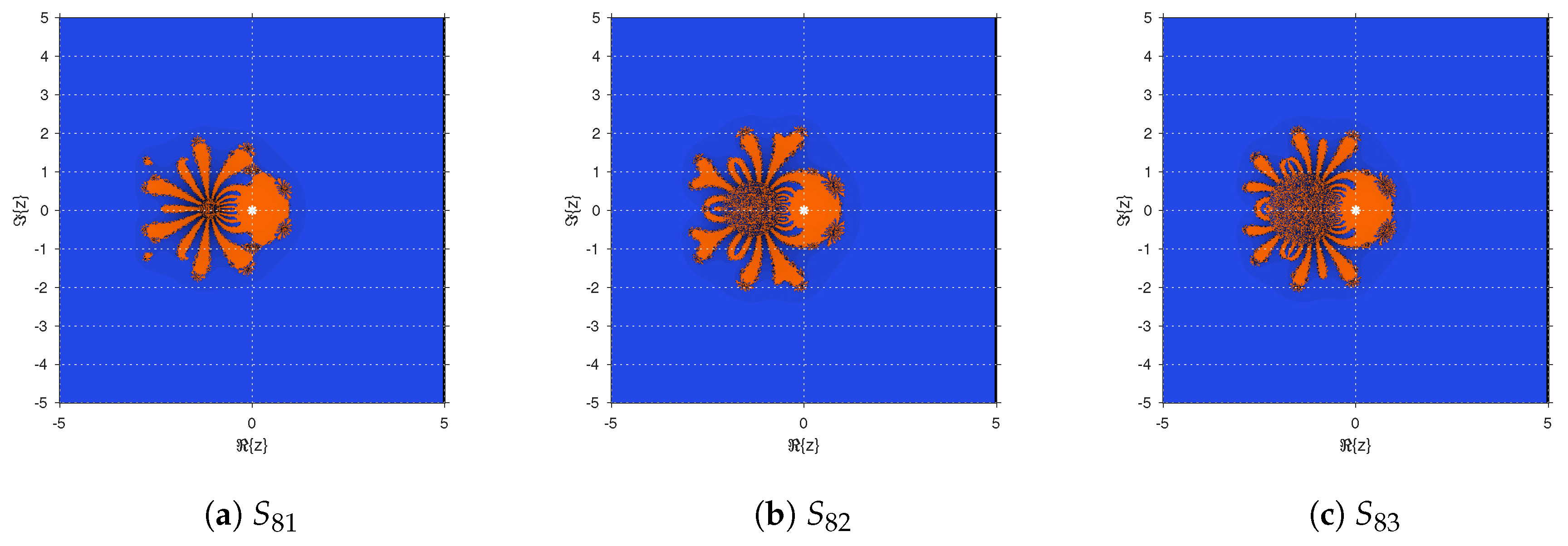
Finally, for the fixed point operators associated with family $M_8$, the solutions of $S_{8i}\left(z\right)=z$ for $i=1,2,3$ give the superattracting fixed points $z_{1,2}^F=z_{1,2}^{\ast }$ and the repelling point $z_3^F=1$. In addition, $S_{81}$ has 28 repelling points. $S_{82}$ and $S_{83}$ have 38 repelling points, corresponding to the roots of polynomials of 28 and 38 degree, respectively, and the strange fixed points $z_{4,5}^F=\frac{1}{2}(-1\pm \sqrt{5})$.

The number of critical points of the fixed point operators $S_{8i}$ are collected in

Table 7. Number of strange fixed points (SFP) and free critical points (FCP) for the methods on quadratic polynomials.

	${\mathit{S}}_4$	${\mathit{S}}_6$	${\mathit{S}}_{81}$	${\mathit{S}}_{82}$	${\mathit{S}}_{83}$
Strange fixed points	7	17	29	41	41
Free critical points	3	29	29	43	29

. In addition, the number of strange fixed points and free critical points are also included in the table for all of the methods.

Figure 2 represents the dynamical planes of the methods $S_{81}$, $S_{82}$ and $S_{83}$. Since the original methods satisfy the Scaling Theorem, the generation of one dynamical plane involves the study of every quadratic polynomial.

There is an intricate region around $z=-1$ in Figure 2a, becoming wider in Figure 2b,c around $z=-1.5$. However, for every initial guess in the three dynamical planes of Figure 2, there is convergence to the roots.

5.4. Dynamics on Cubic Polynomials

The stability of method $M_{41}$ on cubic polynomials is analyzed below. As stated by the authors in [39], the Scaling Theorem reduces the dynamical analysis on cubic polynomials to the study of dynamics on the cubic polynomials $p_0\left(z\right)=z^3$, $p_{+}\left(z\right)=z^3+z$, $p_{-}\left(z\right)=z^3-z$ and the family of polynomials $p_{\gamma }\left(z\right)=z^3+\gamma z+1$. Let us recall that the first one only has the root $z_1^{\ast }=0$, while $p_{+}\left(z\right)$ and $p_{-}\left(z\right)$ have three simple roots: $z_1^{\ast }=0$ and $z_{2,3}^{\ast }=\mp i$ or $z_{2,3}^{\ast }=\mp 1$, respectively. For each $\gamma \in \mathbb{C}$, the polynomial $p_{\gamma }\left(z\right)$ also has three simple roots that depend on the value of $\gamma$. They will be denoted by $z_{1,2,3}^{\ast }\left(\gamma \right)$.

By applying method $M_{41}$ to polynomials $p_0\left(z\right)$, $p_{+}\left(z\right)$ and $p_{-}\left(z\right)$, the fixed point operators obtained are, respectively,

$$\begin{array}{ccc}{S}_{4,0}\left(z\right)=\frac{46z}{81},& S_{4,+}\left(z\right)=\frac{6z^5+36z^7+46z^9}{{(1+3z^2)}^4},& S_{4,-}\left(z\right)=\frac{6z^5-36z^7+46z^9}{{(1-3z^2)}^4}.\end{array}$$

The only fixed point of $S_{4,0}\left(z\right)$ agrees with the root of the polynomial, so it is superattracting, and the operator does not have critical points.

The rest of the fixed point operators have six repelling fixed points, in addition to the roots of the corresponding polynomials: $z_{4,5}^F=\pm \frac{i\sqrt{5}}{5}$ and $z_{6-9}^F=\pm i\sqrt{\frac{1}{7}(3\pm \sqrt{2})}$ for $S_{4,+}\left(z\right)$, and $z_{4,5}^F=\pm \frac{\sqrt{5}}{5}$ and $z_{6-9}^F=\pm \sqrt{\frac{1}{7}(3\pm \sqrt{2})}$ for $S_{4,-}\left(z\right)$.

Regarding the critical points of $S_{4,+}\left(z\right)$ and $S_{4,-}\left(z\right)$, they match with the roots of the polynomials. Moreover, there is the presence of free critical points with values $z_{4,5}^C=\pm i\sqrt{\frac{5}{23}}$ for $S_{4,+}\left(z\right)$ and $z_{4,5}^C=\pm \sqrt{\frac{5}{23}}$ for $S_{4,-}\left(z\right)$.

As for quadratic polynomials, the dynamical planes of method $M_{41}$ when it is applied to the cubic polynomials have been represented in Figure 3. Depending on the roots of each polynomial, the convergence to $z_1^{\ast }=0$ is represented in orange, while the convergence to $z_2^{\ast }$ and $z_3^{\ast }$ is represented in blue and green, respectively. It can be see in Figure 3 that there is full convergence to a root in the three cases. However, there are regions with darker colors that indicate a higher number of iterations until the convergence is achieved.

When method $M_{41}$ is applied on $p_{\gamma }\left(z\right)$, the fixed point function turns into

$$S_{4,\gamma }\left(z\right)=-\frac{{\gamma }^3-46z^9-36\gamma z^7+42z^6-6{\gamma }^2{z}^5+45\gamma z^4+6z^3+12{\gamma }^2{z}^2-1}{{\left(\gamma +3z^2\right)}^4}.$$

The fixed points of $S_{4,\gamma }\left(z\right)$ are the roots of the polynomial $z_{1,2,3}^{\ast }\left(\gamma \right)$, being superattracting, and the strange fixed points $z_{4-9}^F\left(\gamma \right)$ that are the roots of the sixth-degree polynomial $q(z,\gamma )=35z^6+37\gamma z^4+7z^3+11{\gamma }^2{z}^2+\gamma z+{\gamma }^3-1$.

As the asymptotical behavior of $z_4^F\left(\gamma \right),\dots ,z_9^F\left(\gamma \right)$ depends on the value of $\gamma$, the stability planes corresponding to these points are represented in Figure 4. For each strange fixed point, a mesh of $100\times 100$ points covers the values of $\Re \left(\gamma \right)\in [-5,5]$ and $\Im \left(\gamma \right)\in [-5,5]$. The stability plane shows the values for the parameter where $|S_{4,\gamma }^{\prime }\left(z^F\right)|$ is lower or greater than 1, represented in red or green, respectively.

From Figure 4, the strange fixed points are always repelling for $(\Re (\gamma ),\Im (\gamma \left)\right)\in [-5,5]\times [-5,5]$. Then, the only attracting fixed points are the roots of the polynomial. This fact guarantees a better stability of the method.

The solutions of $S_{4,\gamma }^{\prime }\left(z\right)=0$ are the critical points $z_{1,2,3}^C\left(\gamma \right)=z_{1,2,3}^{\ast }\left(\gamma \right)$ and the free critical points $z_4^C=0$ and

$$\begin{array}{ccc}\hfill z_5^C\left(\gamma \right)& =& \frac{{\left(\sqrt{69}\sqrt{125{\gamma }^3+2484}+414\right)}^{2/3}-5\sqrt[3]{69}\gamma }{{69}^{2/3}\sqrt[3]{\sqrt{69}\sqrt{125{\gamma }^3+2484}+414}},\hfill \\ \hfill z_{6,7}^C\left(\gamma \right)& =& \frac{\left(-1\pm i\sqrt{3}\right){\left(\sqrt{69}\sqrt{125{\gamma }^3+2484}+414\right)}^{2/3}+5\sqrt[3]{69}\left(1\pm i\sqrt{3}\right)\gamma }{2{69}^{2/3}\sqrt[3]{\sqrt{69}\sqrt{125{\gamma }^3+2484}+414}}.\hfill \end{array}$$

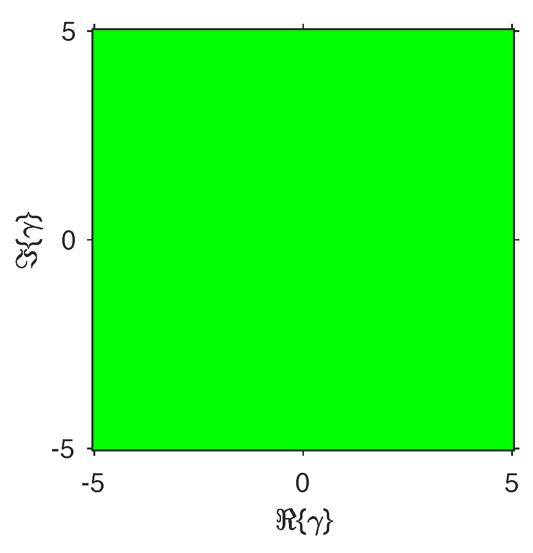
When the fixed point function has dependence on a parameter, another useful representation is the parameters’ plane. This plot is generated in a similar way to the dynamical planes, but, in this case, by iterating the method taking as an initial guess a free critical point and varying the value of $\gamma$ in a complex mesh of values, so each point in the plane represents a method of the family. The parameters’ plane helps to select the values for the parameter that give rise to the methods of the family with more stability.

The parameters’ planes of the four free critical points are shown in Figure 5. Parameter $\gamma$ takes the values of $500\times 500$ points in a complex mesh in the square $[-5,5]\times [-5,5]$. Each point is represented in orange, green or blue when the corresponding method converges to an attracting fixed point. The iterative process ends when the maximum number of 40 iterations is reached, in which case the point is represented in black, or when the method converges as soon as, by the stopping criteria, a difference between two consecutive iterations lower than ${10}^{-6}$ is reached.

For the parameters’ planes in Figure 5, there is not any black region. This guarantees that the corresponding iterative schemes converge to a root of $p_{\gamma }\left(z\right)$ for all the values of $\gamma$.

In order to visualize the basins of attraction of the fixed points, several values of $\gamma$ have been chosen to perform the dynamical planes of method $M_{41}$. These values have been selected from the different regions of convergence observed in the parameters planes. Figure 6, following the same code of colours and stopping criteria as in the other representations, shows the dynamical planes obtained when these values of $\gamma$ are fixed.

As Figure 6 shows, there is not any initial guess that tends to a point different than the roots. This fact guarantees the stability of these methods on the specific case of any cubic polynomial.

6. Conclusions

Two iterative schemes of orders of convergence four and six, and a family of methods of order eight have been introduced. The method of order four and the family of order eight are optimal in the sense of Kung–Traub’s conjecture. The development of the order of convergence of every method has been performed. For every method, we have made a numerical experiment, over both test functions and real engineering problems. In order to analyze the stability of the introduced methods, the dynamical behavior of them has been studied. The results confirm that the methods have wide basins of attraction, guaranteeing the stability over some nonlinear problems.

References

1. Ostrowski, A.M. Solution of Equations and Systems of Equations; Prentice-Hall: Englewood Cliffs, NJ, USA, 1964. [Google Scholar]
2. Cordero, A.; Fardi, M.; Ghasemi, M.; Torregrosa, J.R. Accelerated iterative methods for finding solutions of nonlinear equations and their dynamical behavior. Calcolo 2012, 51, 17–30. [Google Scholar] [CrossRef] [Green Version]
3. Lotfi, T.; Sharifi, S.; Salimi, M.; Siegmund, S. A new class of three-point methods with optimal convergence order eight and its dynamics. Numer. Algor. 2015, 68, 261–288. [Google Scholar] [CrossRef]
4. Chicharro, F.I.; Cordero, A.; Garrido, N.; Torregrosa, J.R. Wide stability in a new family of optimal fourth-order iterative methods. Comput. Math. Meth. 2019, 1, e1023. [Google Scholar] [CrossRef]
5. Chicharro, F.I.; Cordero, A.; Torregrosa, J.R. Dynamics of iterative families with memory based on weight functions procedure. J. Comput. Appl. Math. 2019, 354, 286–298. [Google Scholar] [CrossRef]
6. Sharma, R.; Bahl, A. An optimal fourth order iterative method for solving nonlinear equations and its dynamics. J. Complex Anal. 2015, 2015, 259167. [Google Scholar] [CrossRef]
7. Sharifi, M.; Babajee, D.K.R.; Soleymani, F. Finding solutions of nonlinear equations by a class of optimal methods. Comput. Math. Appl. 2012, 63, 764–774. [Google Scholar] [CrossRef]
8. Kung, H.T.; Traub, J.F. Optimal order of one-point and multipoint iterations. J. Assoc. Comput. Mach. 1974, 21, 643–651. [Google Scholar] [CrossRef]
9. Potra, F.A.; Pták, V. Nondiscrete induction and iterative processes. Res. Notes Math. 1984, 103, 112–119. [Google Scholar]
10. Amat, S.; Busquier, S.; Plaza, S. Review of some iterative root finding methods from a dynamical point of view. Scientia 2004, 10, 3–35. [Google Scholar]
11. Babajee, D.K.R.; Cordero, A.; Soleymani, F.; Torregrosa, J.R. On improved three-step schemes with high efficiency index and their dynamics. Numer. Algor. 2014, 65, 153–169. [Google Scholar] [CrossRef]
12. Chicharro, F.I.; Cordero, A.; Torregrosa, J.R.; Vassileva, M.P. King-type derivative-free iterative families: Real and memory dynamics. Complexity 2017, 2017, 2713145. [Google Scholar] [CrossRef]
13. Cordero, A.; Feng, L.; Magreñán, Á.A.; Torregrosa, J.R. A new fourth order family for solving nonlinear problems and its dynamics. J. Math. Chem. 2015, 53, 893–910. [Google Scholar] [CrossRef]
14. Scott, M.; Neta, B.; Chun, C. Basin attractors for various methods. Appl. Math. Comput. 2011, 218, 2584–2599. [Google Scholar] [CrossRef]
15. Varona, J.L. Graphic and numerical comparison between iterative methods. Math. Intell. 2002, 24, 37–46. [Google Scholar] [CrossRef]
16. Vrscay, E.R.; Gilbert, W.J. Extraneous fixed points, basin boundaries and chaotic dynamics for Schroder and Konig rational iteration functions. Numer. Math. 1988, 52, 1–16. [Google Scholar] [CrossRef]
17. Alexander, D.S. A History of Complex Dynamics: From Schröder to Fatou and Julia; Vieweg & Teubner Verlag: Wiesbaden, Germany, 1994. [Google Scholar]
18. Beardon, A.F. Iteration of Rational Functions; Springer: New York, NY, USA, 2000. [Google Scholar]
19. Blanchard, P. The dynamics of Newton’s method. Proc. Sympos. Appl. Math. 1994, 49, 139–154. [Google Scholar]
20. Carleson, L.; Gamelin, T.W. Complex Dynamics; Springer-Verlag: New York, NY, USA, 1992. [Google Scholar]
21. Devaney, R.L. An Introduction to Chaotic Dynamical Systems; Addison-Wesley: Redwood City, CA, USA, 1989. [Google Scholar]
22. Matthies, G.; Salimi, M.; Sharifi, S.; Varona, J.L. An optimal class of eighth-order iterative methods based on Kung and Traub’s method with its dynamics. arXiv 2015, arXiv:1508.01748v1. [Google Scholar]
23. Cordero, A.; Torregrosa, J.R. Variants of Newton’s method using fifth order quadrature formulas. Appl. Math. Comput. 2007, 190, 686–698. [Google Scholar] [CrossRef]
24. Jarratt, P. Some efficient fourth order multipoint methods for solving equations. BIT 1969, 9, 119–124. [Google Scholar] [CrossRef]
25. Neta, B. A sixth-order family of methods for nonlinear equations. Int. J. Comput. Math. 1979, 7, 157–161. [Google Scholar] [CrossRef]
26. Grau, M.; Díaz-Barrero, J.L. An improvement to Ostrowski root-finding method. Appl. Math. Comput. 2006, 173, 450–456. [Google Scholar] [CrossRef]
27. Sharma, J.R.; Guha, R.K. A family of modified Ostrowski’s methods with accelerated sixth order convergence. Appl. Math. Comput. 2007, 190, 111–115. [Google Scholar]
28. Chun, C.; Neta, B. A new sixth-order scheme for nonlinear equations. Appl. Math. Lett. 2012, 25, 185–189. [Google Scholar] [CrossRef] [Green Version]
29. Chun, C.; Lee, M.Y. A new optimal eighth-order family of iterative methods for the solution of nonlinear equations. Appl. Math. Comput. 2013, 223, 506–519. [Google Scholar] [CrossRef]
30. Chapra, S.C.; Canale, R.C. Numerical Methods for Engineers; McGraw Hills Education: New York, NY, USA, 2015. [Google Scholar]
31. Brkić, D. A note on explicit approximations to Colebrook’s friction factor in rough pipes under highly turbulent cases. Int. J. Heat Mass tramsf. 2016, 93, 513–515. [Google Scholar] [CrossRef]
32. Wang, J.; Pang, Y.; Zhang, Y. Limits of solutions to the isentropic Euler equations for van der Waals gas. Int. J. Nonlinear Sci. Numer. Simul. 2019, 20, 461–473. [Google Scholar] [CrossRef]
33. Gates, D.J.; Penrose, O. The van der Waals limit for classical systems. I. A variational principle. Comm. Math. Phys. 1969, 15, 255–276. [Google Scholar] [CrossRef]
34. Gates, D.J.; Penrose, O. The van der Waals limit for classical systems. II. Existence and continuity of the canonical pressure. Comm. Math. Phys. 1970, 16, 231–237. [Google Scholar] [CrossRef]
35. Gates, D.J.; Penrose, O. The van der Waals limit for classical systems. III. Deviation from the van der Waals-Maxwell theory. Comm. Math. Phys. 1970, 17, 194–209. [Google Scholar] [CrossRef]
36. Blanchard, P. Complex analytic dynamics on the Riemann sphere. Bull. Am. Math. Soc. 1984, 11, 85–141. [Google Scholar] [CrossRef] [Green Version]
37. Schlag, W. A Course in Complex Analysis and Riemann Surfaces; American Mathematical Society: Providence, RI, USA, 2014. [Google Scholar]
38. Chicharro, F.I.; Cordero, A.; Torregrosa, J.R. Drawing dynamical and parameters planes of iterative families and methods. Sci. World J. 2013, 2013, 780153. [Google Scholar] [CrossRef] [PubMed]
39. Amat, S.; Busquier, S.; Plaza, S. Chaotic dynamics of a third-order Newton-type method. J. Math. Anal. Appl. 2010, 366, 24–32. [Google Scholar] [CrossRef] [Green Version]
Figure 1. Dynamical planes of methods S 4 and S 6 .
Mathematics 07 00942 g001
Figure 2. Dynamical planes of methods S 8 i , i = 1 , 2 , 3 .
Mathematics 07 00942 g002
Figure 3. Dynamical planes of method M 41 on polynomials p 0 ( z ) , p + ( z ) and p ( z ) .
Mathematics 07 00942 g003
Figure 4. Stability planes of z 4 9 F ( γ ) .
Mathematics 07 00942 g004
Figure 5. Parameter planes of the critical points of method M 41 on p γ ( z ) .
Mathematics 07 00942 g005
Figure 6. Dynamical planes for method M 41 on p γ ( z ) for different values of γ .
Mathematics 07 00942 g006