Integrated Vendor–Buyer Lot-Sizing Model with Transportation and Quality Improvement Consideration under Just-in-Time Problem

Abstract

This paper deals with the problem of transportation and quality within a Just-in-Time (JIT) inventory replenishment system. Formerly, transportation and quality problem are often modelled separately in most integrated inventory lot-sizing models. Hence, this paper develops an integrated vendor-buyer lot-sizing model by considering transportation and quality improvements into a JIT environment. The model is developed for minimising a total vendor-buyer system cost by optimising decisions such as delivery quantity, production batch, number of shipments, and process quality. Numerical examples and sensitivity analysis are provided to illustrate the proposed model. The developed model was also compared with an enumeration method to analyse the effectiveness of the proposed model to find the optimum solution. The results emphasise that the proposed model contributes to a new approach and obtains a near optimum solution for inventory replenishment decisions. The results are also beneficial to JIT practices as the model can improve the transport payload and reduce the chance of defective products and improving quality-related costs.

1. Introduction

The application of the Just-in-Time (JIT) purchasing system has a tremendous effect on helping eliminate waste through various issues such as consistency in improving quality and minimising inventory costs by frequent deliveries in small quantities. Conversely, the application of JIT purchasing has a direct effect on buyers by reducing costs as their order is typically made ‘to order’ on an as-required basis in small quantity deliveries [1]. The buyers are left to decide how much they requires and when they need it, so this purchasing process may lead to an increased cost to the vendors as they have now lost control [2,3].

To deal with this problem, Goyal [4] proposed a vendor-buyer integrated model as opposed to a buyer’s independent decision in inventory replenishment. Based on previous studies, most integrated inventory lot-sizing models propose solutions to minimise costs in the supply chain [5]. To encourage the formulation of integrated systems, cost saving within an integrated supply chain model are fully realised through revenue sharing between vendor and buyer by agreeing to a joint purchasing policy, often with a side payment [6]. In practice, there must be understanding and trustworthy collaboration between the members of the chain to achieve an integrated supply chain.

Integrated models have also been linked to solve problems that arise from frequent deliveries in small quantities with a high-quality product [7,8]. Generally, the JIT buyer can reduce inventory costs due to frequent deliveries in small quantities, but this might result in an increased transportation costs for the buyer [9,10]. It is also possible to have shipments in Less-than-Truck Load (LTL) with low utilisation of the transportation payload [11]. Consequently, companies need to determine how much and how often inventory replenishment takes place to optimise their transportation cost. In order to make a significant impact on cost reduction, inventory replenishment decisions need to consider transportation costs as an element within the supply chain cost calculations [12]. Therefore, researchers and practitioners have been dealing with such issues to investigate the effect of transportation cost on the integrated vendor-buyer lot-sizing model.

In addition to the transportation problem, quality can become a crucial issue in a production system [13,14,15]. The product from a vendor is not always 100% acceptable to the buyer [9]. Defective products can be generated during production runs, and additional costs are incurred for rejecting, reworking, and repairing the product. Moreover, there are external costs including returning the product, refunding or exchanging, or resolving customer complaints while trying to retain customer loyalty [16]. As a result, these failure costs can significantly affect a firm’s profit in the short and long term. Consequently, investment in quality control and capability is required so that the product is fit for purpose [17,18]. Therefore, quality and production need to be linked in the model to analyse their effects on inventory replenishment decisions.

Transportation and quality problems are the major focus within this paper which develops a vendor-buyer integrated model including transportation and quality cost improvements to determine an optimal inventory replenishment decision. The aim of the model is to reduce the total cost of the setup/order, with fixed and variable transportation, inventory replenishment, and quality improvement by deciding the optimal delivery quantity, the batch production quantity, the number of deliveries, and the process quality.

Section 2 of the paper briefly reviews the literature that relates to the extension of integrated inventory model with transportation and quality issues. Section 2 also presents the contribution of this study. Section 3 develops mathematical modelling on transportation cost and quality improvement and the associated solution procedures. Section 4 presents numerical examples to illustrate and examine the feasibility of the proposed procedure for the model. A validation-based sensitivity analysis has been conducted to examine the effect of the model’s parameters on the model solution, which is discussed in Section 5. In order to analyse the proposed model for achieving the best solution, experimentation is reported in Section 6. The last section summarises the results and makes recommendations for future research.

2. Literature Review

2.1. Integrated Vendor-Buyer Inventory Model with Transportation

In recent years, researchers and practitioners have been dealing with the effect of transportation cost on the integrated inventory model. Nie et al. [7] considered the transportation function of Swenseth and Godfrey [12] with regard to the shipping weight to find the optimal inventory decision for two transportation modes, including a Full Truck Load (FTL) and LTL. In practice, the FTL mode denotes a constant charge per shipment with a full container load at a given capacity. Meanwhile, the cost of an LTL mode is based on the base rates, shipping weight, distance, and discount. Hence, they proposed an analytical method to solve the problem for each transportation mode and a heuristic method to find the optimal inventory decision between the solution of FTL and LTL mode that improve the performance of the model.

Ertogral et al. [19] considered an all-unit-discount transportation cost structure as a function of the shipment size. They proposed three solution procedures based on analytical method for solving the models. Chen and Sarker [9] modified the transportation function of Swenseth and Godfrey [12] by taking into account the distance travelled and analysed its effect on delivery quantity, batch production quantity, and number of shipments under the consideration of LTL mode. Meanwhile, the study also proposed a solution procedure to solve the problem of incapacitated and capacitated models analytically, which are related to the truckload capacity. Mutlu and Çetinkaya [20] considered a common carrier rate as a function of the shipment quantity to determine the order-up-to-level for replenishing the inventory and the dispatch cycle length. The study contributed to propose new analytical models in obtaining solutions for the model under the common carrier rates. Madadi et al. [21] developed integrated inventory models with transportation costs as the function of distance travelled for the case of a centralised ordering model. The study proposed analytical method to solve the centralised model and reach reasonable cost savings.

Lee and Fu [22] estimated the transportation cost as a function of the delivery quantity using linear regression and combined it into the integrated model. Lee and Fu [23] also extended their study by developing an integrated production–delivery quantity model with the transportation cost as a power function with the actual shipping rate data obtained from the shipping company. For both study of Lee and Fu [22] and Lee and Fu [23] proposed solution procedure based on analytical method to find the optimum solution of production and delivery quantities.

Leuveano et al. [24] incorporated transportation as the function of shipping weight and distance into an integrated model. However, the transportation function only deals with LTL shipments. Rahman et al. [2] also developed an integrated inventory lot-sizing model that covers both LTL shipment and FTL shipment. The proposed models provide a heuristic approach to find an optimal solution when the transportation mode is restricted to FTL and LTL shipments. Sarkar et al. [25] analysed the effect of variable transportation as the function of lot size in a three-echelon supply chain model to make the model more realistic than in previous studies. The study employed algebraic approach to find the closed-form solution.

2.2. Integrated Vendor-Buyer Inventory Model with Quality Improvement

The provision of high-quality products has also been a major challenge in the production system. For that reason, JIT systems are continuously emphasising on “zero waste” by choosing a vendor that consistently produces higher quality products [1]. However, products are not always 100% acceptable to the buyer [9]. In this case, these defective products are generated and have an impact on the manufacturing process and will lead to a disruption in the inventory management systems within the supply chain. Accordingly, the vendor incurs additional costs for reworking a product in order to restore its quality [16]. To improve the process quality, investment in quality improvement and production need to be linked in the model to analyse their effects on inventory replenishment decisions. Some works studied the effect of quality improvement in the integrated inventory lot-sizing model to get a better decision.

Affisco et al. [26] attempted to include investment in quality improvement into an integrated model for increasing the probability of consistent quality products. As a consequence, the optimal lot size decreases as the process quality increases and the quality-related cost reduces. Liu and Çetinkaya [27] modified a particular form of the investment function proposed by Affisco et al. [26] because it did not represent the practice in the real world. This is because the investment function is a concave function, and the results obtained in the model of Affisco et al. [27] are invalid. Yang and Pan [28] incorporated the investment in quality improvement to reduce the probability of defective products, thus resulting in a smaller lot while increasing the number of shipments to the buyer. Ouyang et al. [29] extended the model of Yang and Pan [28] by involving the shortage and re-order point parameters. As a result, the probability of defective products is smaller than in the model by Yang and Pan [28].

Majumder et al. [18] developed an integrated model with quality improvement and setup reduction. To improve product quality and setup costs, a fund investment is included in the model and investigate its effect on inventory replenishment decision. Sarkar et al. [30] developed an integrated single vendor and multi-buyer model with a variable production rate that affected the product quality, concluding that a high production rate causes poor product quality. Therefore, the production rate is treated as a decision variable in their model. Dey and Sarkar [31] developed a two-echelon of a single vendor and multi-retailers model that considers the reduction of the defective products and setup cost through investments. All previous studies that developed an integrated inventory model with quality improvement proposed their solution procedures based on analytical method to find global optimal inventory decision to reduce total cost system of setup, order, inventory, and quality.

2.3. Gap Summary

The above works mostly discussed integrated vendor-buyer lot-sizing models with transportation and quality separately. Unlike previous researches, transportation and quality problems are important to be addressed and become major focus within this paper. Therefore, this research aims to fill this gap by developing a mathematical model of integrated vendor-buyer lot-sizing including transportation and quality improvements to determine an optimal inventory replenishment decision. The objective of the model is to reduce the total cost of the setup/order with fixed and variable transportation, inventory replenishment, and quality improvement by deciding the optimal delivery quantity, the batch production quantity, the number of deliveries, and the process quality. This study also proposes a solution procedure based on an analytical method and a heuristic method to find optimum inventory replenishment decision for solving transportation and quality problems.

3. Model Formulation

This section elaborates problem definition, notation, assumptions, and the mathematical model and its solution procedures.

3.1. Problem Definition

A model consisting of a single vendor and a single buyer which undertake supply chain activities under a JIT environment is presented in Figure 1.

The figure above shows a buyer orders a product from a vendor and frequently orders in smaller lot sizes when it comes to higher quality products. Moreover, a vendor uses the Economic Manufacturing Quantity (EMQ) to manufacture the products with a single setup and with multiple shipment strategies so that the order is produced in a number of equal-sized shipments. In the production process, quality becomes the major problem faced by the vendor. Probability of defective products occurs due to an imperfect production process. Generally, the vendor conducts an inspection to screen his products produced to identify the initial probability of defective products. In order to reduce the number of defective products, the vendor attempts to invest in quality improvement. This investment is used to improve the quality of production process by assuring the product produced meets the quality standard. Therefore, the impact of this investment is to increase the probability of good products in production process before the transportation.

In the process of delivering the products, the buyer incurs variable transportation costs with regard to the total shipping weight, which is dependent on the given truckload capacity. Since this study focuses on JIT environment which buyer frequently orders in smaller lot sizes, then products are carried with LTL shipment. Moreover, two transportation problems might occur: incapacitated and capacitated. ‘Incapacitated’ is the problem that occurs when the total shipping weight may not exceed the amount of the truckload capacity. ‘Capacitated’ occurs when the total shipping weight exceeds truckload capacity. Therefore, this study attempts to optimize transportation payload under LTL shipment and two transportation problems (incapacitated and capacitated). When the products arrive at the buyer’ stage, a delivery inspection is conducted, and any defective products are detected at this stage. The good products are kept in the warehouse, and the defective products are immediately returned to the vendor and replaced at a cost. For this reason, the vendor requires an investment in quality improvement to increase production of superior products, thereby reducing the quality check cost for returning and replacing defective products.

To utilise the transportation payload and improve the quality, this study incorporated the transportation cost and quality improvement investment into the integrated inventory decision model. The model solution is based on five aspects: total cost, delivery quantity, the number of shipments, production batch, and process quality.

3.2. Notation and Assumption

The following are the notations and assumptions used throughout this paper:

3.2.1. Notation

The following notations used to establish the proposed model are shown in

Table 1. Notations of the model.

Parameter	Description
$\mathrm{D}$	Demand rate of the buyer (unit/year),
$\mathrm{P}$	The production rate of the vendor (unit/year),
$\mathrm{A}$	Order cost per order (buyer) ($/order),
$\mathrm{S}$	Setup cost per setup (vendor) ($/setup),
$H_v$	Vendor holding cost ($/unit/year),
$H_b$	Buyer holding cost ($/unit/year),
$C_m$	Vendor’s returning, repairing and replacement cost as a result of defective products ($/unit),
$C_n$	Buyer’s full inspection cost ($/unit),
$F_0$	Fixed transportation cost for preparing each shipment ($/delivery),
$F_x$	The freight rate in dollars per pound per mile at full truckload capacity ($/lb),
$F_y$	The freight rate in dollars per pound for the partial load ($/lb),
$\mathsf{\alpha }$	Discount factor,
$\mathrm{w}$	The weight of a part (lb),
$W_x$	Full truckload capacity (lbs),
$W_y$	Actual shipping weight (lbs) ${(W}_y=\mathrm{q}\mathrm{w})$,
${VTc}_a$	Total variable transportation cost as the result of querying the actual freight rate schedule of the total shipping weight ($/shipments),
${VTc}_b$	Total variable transportation cost as a function of shipping weight ($/shipments),
$\mathsf{\theta }$	The probability of defective products,
${\stackrel{-}{p}}_0$	The initial probability of good products ($1-\mathsf{\theta }$),
$\mathrm{i}$	The fractional per unit time cost of capital,
${TC}_v$	Vendor total cost ($/year),
${TC}_{b1}$	Buyer total cost with consideration of ${VTC}_b$ ($/year),
${TC}_j$	The total cost of vendor and buyer ($/year),
${TC}_{j0}$	The total cost of the vendor and buyer with consideration of ${VTC}_a$ ($/year),
${TC}_{j1}$	The total cost of the vendor and buyer with consideration of ${VTC}_b$($/year),
Decision variables
$\mathrm{q}$	Equal-sized delivery/order quantity (unit) $(\mathrm{q}=\mathrm{Q}/\stackrel{-}{p}\mathrm{m})$,
$\mathrm{m}$	Number of shipments,
$\mathrm{Q}$	Production batch quantity (units) $(\mathrm{Q}=\mathrm{q}\stackrel{-}{p}\mathrm{m})$,
$\stackrel{-}{p}$	The probability of good products.

.

3.2.2. Assumptions

The assumptions made in this paper for simplifying the proposed model are as follows:

• This integrated model consists of a single vendor and a single buyer in a long-term partnership.
• One vendor supplies a single product to the buyer.
• Demand, production, and delivery lead time are assumed to be deterministic.
• The vendor uses a finite production rate P, and a vendor’s production rate that is greater than the demand rate $\mathrm{P}>\mathrm{D}$.
• The probabilities of defective and good products are known.
• The buyer’s holding cost is greater than the vendor’s holding cost $H_b{>H}_v$.
• The shipment policy can be carried out during the production period, and the production batch is delivered in equal-sized shipments.
• Shortages and backorders are not allowed. Any shortage occurs due to defective products detected at the buyer’s site before they go into buyer’s warehouse are immediately returned and replaced by the vendor at cost. To avoid shortage, the vendor has a production rate that is greater than demand rate of buyer. Therefore, the vendor is prepared immediately if there were defective products found at the buyer’s site. This situation mostly happens in manufacturing industries.
• The transportation cost for returning the defective products (reverse logistic) to the vendor is negligible in detail. This model assumes that the reverse logistics cost is part of replacing and returning defective products to the vendor.

3.3. Mathematical Model

First, a graphical illustration of the inventory replenishment between a single vendor and a single buyer under quality issue is given in Figure 2. As presented in Figure 2, a vendor produces a production batch $\mathrm{Q}$ in one setup and ships it with equal-sized delivery/order quantity $\mathrm{q}$ over multiple shipments m under the deterministic rate of demand $\mathrm{D}$ and production $\mathrm{P}$. Hence, a production batch is expressed as $\mathrm{Q}=\mathrm{m}\mathrm{q}$. This approach is consistent with the JIT implementation, which emphasises multiple shipments in small lots. Each $\mathrm{q}$ contain the probability of defective products $\mathsf{\theta }$ and the probability of good products become $\stackrel{-}{p}=1-\mathsf{\theta }$. Based on Figure 2, a vendor produces $\mathrm{q}$ with $\stackrel{-}{p}$ at the time ${\mathrm{T}}_0$ and stores it until the products sent at the time ${\mathrm{T}}_1$. In this case, the total production batch can be reformulated as $\mathrm{Q}=\mathrm{m}\mathrm{q}\stackrel{-}{p}$. Moreover, the remaining products produced are $\left(m-1\right)\mathrm{q}$$\stackrel{-}{p}$, with the time for producing the order being $(\mathrm{m}-1)\mathrm{q}\stackrel{-}{p}/\mathrm{D}$ years until time $T_e$. This means that the vendor only ships the remaining delivery quantity to the buyer at $T_2,$… ${,T}_n$−1 ${,T}_n$. After conducting a full inspection of the incoming products, the buyer only obtains good quality products as $\mathrm{q}\stackrel{-}{p}$over time. Moreover, the inventory cost of the buyer is computed based on good quality products from a vendor.

The integrated model is comprised of the vendor and buyer mathematical cost functions. At first, these cost functions were explained independently in order to see how the integrated model was developed.

3.3.1. Vendor Cost Function

The cost function of the vendor was formulated as follows:

$${TC}_v\left(q,m,\stackrel{-}{p}\right)=\frac{D}{q\stackrel{-}{p}}\left(\frac{S}{m}{+F}_0\right)+\frac{q\stackrel{-}{p}}{2}\left(m\left(1-\frac{D}{P}\right)-1+\frac{2D}{P}\right)H_v+\frac{D}{\stackrel{-}{p}}\left(1-\stackrel{-}{p}\right)C_m.$$

(1)

The vendor cost function included the setup cost, fixed transport cost, holding cost, and returning and replacement cost. The expression for the holding cost was adopted from Joglekar [32] (See Appendix A for derivation). Moreover, the total amount of defective products $\frac{D}{\stackrel{-}{p}}\left(1-\stackrel{-}{p}\right)$ was replaced by the vendor at a cost of $C_m$unit.

3.3.2. Buyer Cost Function

The buyer cost function was expressed as follows:

$${TC}_{b0}\left(q,\stackrel{-}{p}\right)=\frac{D}{q\stackrel{-}{p}}\mathrm{A}+\frac{q\stackrel{-}{p}}{2}{H}_b+\frac{D}{\stackrel{-}{p}}{C}_n{+VTC}_a.$$

(2)

The buyer cost function consisted of the ordering cost, holding cost, inspection cost, and variable transportation cost. The buyer will screen the incoming material by implementing a full inspection that incurs cost $C_n$. A variable transportation cost ${VTC}_a$ is paid by the buyer, where the cost is calculated by querying the actual freight rate of the total shipping weight. In this case, to include variable transportation cost into the model, it must be a function that estimates the actual freight rate with regard to the shipping weight. Hence, this paper adopted the variable transportation function of Swenseth and Godfrey [12], which is given as follows:

$${VTC}_b{=F}_y\mathrm{Dw}.$$

(3)

Since this paper is consistent with a JIT implementation, where a buyer orders in small quantities (equal sizes) over multiple shipments, then the truck that carries the products is often moved with the LTL shipment. For that situation, the determination of $F_y$should simultaneously emulate the LTL shipment and the actual freight rates. Again, this paper adopted the function of Swenseth and Godfrey [12] that can emulate the LTL shipment, namely adjusting the inverse, as formulated in Equation (4). The adjusted inverse function took the form of a step function, which decreased as the shipping weight increased.

$$F_y{=F}_x{+\mathsf{\alpha }F}_x\left[\frac{W_x{-W}_y}{W_y}\right],$$

(4)

where α is a discount factor that represents a value between 0 and 1 for hauling the LTL or a small shipment, and $W_y$is the actual shipping decision ($W_y$ = $\mathrm{q}$ $\mathrm{w}$). Thus, the total variable transportation cost function can be elaborated based on the adjusted inverse function by substituting Equation (4) into Equation (3) as

$${VTC}_b=\left[F_x{+\alpha F}_x\left[\frac{W_x{-W}_y}{W_y}\right]\right]\mathrm{Dw}=\frac{D}{q\stackrel{-}{p}}{\mathsf{\alpha }F}_x{W}_x+\mathrm{Dw}\left(1-\alpha \right)F_x.$$

(5)

Therefore, there are two cost functions of the buyer that can be formulated when considering variable transportation cost. First, the total buyer cost function that considers actual freight (see Equation (2)), and second, the total buyer cost function that could emulate LTL shipment is as follows:

$${TC}_{b1}\left(q,\stackrel{-}{p}\right)=\frac{D}{q\stackrel{-}{p}}\mathrm{A}+\frac{q\stackrel{-}{p}}{2}{H}_b+\frac{D}{\stackrel{-}{p}}{C}_n+\frac{D}{q\stackrel{-}{p}}{\mathsf{\alpha }F}_x{W}_x+\mathrm{Dw}\left(1-\alpha \right)F_x.$$

(6)

3.3.3. Integrated Inventory Model with Transportation Costs

The integrated inventory model is composed of vendor and buyer cost functions. Since the variable transportation cost is typically calculated based on the shipping weight, two integrated inventory models were also derived—one that considered the actual freight schedule ${VTC}_a,$and the other that incorporated a variable transportation cost function ${VTC}_b$ that could emulate the LTL shipment as well as a representation of the actual freight rate. Hence, an integrated inventory model with an actual freight rate schedule can be formulated by combining Equations (1) and (2) as follows:

$${TC}_{j0}\left(q,m,\stackrel{-}{p}\right)=\frac{D}{q\stackrel{-}{p}}\left(A+\frac{S}{m}{+F}_0\right)+\frac{q\stackrel{-}{p}}{2}\left(\left(m\left(1-\frac{D}{P}\right)-1+\frac{2D}{P}\right)H_v{+H}_b\right)+\frac{D}{\stackrel{-}{p}}\left(\left(1-\stackrel{-}{p}\right)C_m{+C}_n\right){+VTC}_a.$$

(7)

Moreover, an integrated inventory model with a variable transportation function can be formulated by combining Equations (1) and (6) is as follows:

$$\begin{array}{ll}{TC}_{j1}\left(q,m,\stackrel{-}{p}\right)& =\frac{D}{q\stackrel{-}{p}}\left(A+\frac{S}{m}{+F}_0\right)+\frac{q\stackrel{-}{p}}{2}\left(\left(m\left(1-\frac{D}{P}\right)-1+\frac{2D}{P}\right)H_v{+H}_b\right)+\frac{D}{\stackrel{-}{p}}\left(\left(1-\stackrel{-}{p}\right)C_m{+C}_n\right)\\ & +\frac{D}{q\stackrel{-}{p}}{\mathsf{\alpha }F}_x{W}_x+\mathrm{Dw}\left(1-\alpha \right)F_x.\end{array}$$

(8)

3.3.4. Quality Improvement

In addition to transportation costs, the integrated model was also formulated by considering the quality issue. As mentioned earlier, small lot sizes are produced with high-quality products in the JIT implementation. Hence, with such characteristics, this study incorporated quality improvement into the model for achieving the goal of the JIT. Now, it is necessary to discuss the quality aspect in Equations (7) and (8). The value of $\stackrel{-}{p}$ is the solution that leads to the quality-adjusted optimal lot size [27]. Consider a restriction to Equations (15) and (16), where $0\le {\overline{p}}_0\le \stackrel{-}{p}\le 1.$ This shows that if $\stackrel{-}{p}\le 1$, then a vendor requires an investment function on quality improvement to improve the production process so that $\stackrel{-}{p}$ is fully expected to be near the value of 1 (perfect quality). For instance, to reduce probability of defective products from 0.1 to 0.05 may need an investment of $200. In this case, this investment has a potential impact associated with changing the initial quality $\left({\stackrel{-}{p}}_0\right)$ [26]. Therefore, this paper incorporated the quality investment function of Liu and Çetinkaya [27] into the integrated model, which is expressed as follows:

$$\mathrm{f}\left(\stackrel{-}{p}\right){=\mathrm{i}a}_{\stackrel{-}{p}},$$

(9)

where $\mathrm{i}$ is the fractional per unit time cost of capital, and $a_{\stackrel{-}{p}}$represents the cost of investment as a function of $\stackrel{-}{p}$.

Moreover, to obtain the function that represents the practical quality improvement investment, Liu and Çetinkaya [27] revised the exponential growth function of investment of Affisco et al. [26] to become

$$\left(1-\stackrel{-}{p}\right)=\left({1-\stackrel{-}{p}}_0\right)e^{-\Delta a_{\stackrel{-}{p}}},$$

(10)

s.t. $0\le {\overline{p}}_0\le \overline{p}\le 1.$ where $\Delta >0$ is the technology coefficient representing the percentage increase in $\stackrel{-}{p}$ per dollar increase in $a_{\stackrel{-}{p}}\left(\stackrel{-}{p}\right)$. To obtain a cost of investment as a function of $\stackrel{-}{p}$, Equation (10) was rewritten as follows:

$$a_{\stackrel{-}{p}}\left(\stackrel{-}{p}\right){=\beta }^{\prime }-\mathsf{\gamma }\ln \left(1-\stackrel{-}{p}\right),$$

(11)

where ${\beta }^{\prime }{=\ln (1-\stackrel{-}{p}}_0)/\Delta >0$, $\mathsf{\gamma }=1/\Delta$, $0\le {\stackrel{-}{p}}_0\le \stackrel{-}{p}\le 1$, and a functioning $a_{\stackrel{-}{p}}\left(\stackrel{-}{p}\right)$is convex with respect to the increase in $\stackrel{-}{p}$ because

$$\begin{gathered} \frac{\partial a_{\stackrel{-}{p}}\left(\stackrel{-}{p}\right)}{\partial \stackrel{-}{p}}=\frac{\gamma }{1-\stackrel{-}{p}}>0,\mathrm{and} \\ \frac{{\partial }^2{a}_{\stackrel{-}{p}}\left(\stackrel{-}{p}\right)}{\partial {\stackrel{-}{p}}^2}=\frac{\gamma }{{\left(1-\stackrel{-}{p}\right)}^2}>0. \end{gathered}$$

(12)

Hence, the quality investment function from Liu and Çetinkaya [27] that was used in this paper was obtained by substituting Equation (11) into Equation (9) as

$$\mathrm{f}\left(\stackrel{-}{p}\right)=\mathrm{i}\left({\beta }^{\prime }-\gamma ln\left(1-\stackrel{-}{p}\right)\right).$$

(13)

3.3.5. Integrated Inventory Model with Transportation Cost and Quality Improvement

Next, this paper further investigated the potential impact of incorporating the transportation cost and investment in quality improvement into the total cost of performance and the optimal solution. Accordingly, the integrated inventory model in Equations (7) and (8) was rewritten to incorporate quality improvement. For variable transportation costs with querying actual freight rate, the integrated inventory model can be formulated by combining Equations (7) and (13) to become:

$$\begin{array}{ll}{TC}_{j0}\left(q,m,\stackrel{-}{p}\right)=& \frac{D}{q\stackrel{-}{p}}\left(A+\frac{S}{m}{+F}_0\right)+\frac{q\stackrel{-}{p}}{2}\left(\left(m\left(1-\frac{D}{P}\right)-1+\frac{2D}{P}\right)H_v{+H}_b\right)+\frac{D}{\stackrel{-}{p}}\left(\left(1-\stackrel{-}{p}\right)C_m{+C}_n\right)\\ & +\mathrm{i}\left({\beta }^{\prime }-\gamma ln\left(1-\stackrel{-}{p}\right)\right){+VTC}_a.\end{array}$$

(14)

In contrast to Equation (14), Equation (15) included the total cost function, the decomposition of ${VTC}_a$, and the quality investment function by combining Equations (8) and (13), to obtain

$$\begin{array}{ll}{TC}_{j1}\left(q,m,\stackrel{-}{p}\right)=& \frac{D}{q\stackrel{-}{p}}\left(A+\frac{S}{m}{+F}_0{+\alpha F}_x{W}_x\right)+\frac{q\stackrel{-}{p}}{2}\left(\left(m\left(1-\frac{D}{P}\right)-1+\frac{2D}{P}\right)H_v{+H}_b\right)+\\ & \frac{D}{\stackrel{-}{p}}\left(\left(1-\stackrel{-}{p}\right)C_m{+C}_n\right)+\mathrm{Dw}\left(1-\alpha \right)F_x+\mathrm{i}\left({\beta }^{\prime }-\gamma ln\left(1-\stackrel{-}{p}\right)\right).\end{array}$$

(15)

For Equations (14) and (15), the problem was that

$$\mathrm{Min}{TC}_j\left(q,m,\stackrel{-}{p}\right)$$

s.t. $\mathrm{q}>0;\mathrm{m}>0;\mathrm{q}$ and $\mathrm{m}$ are integer values; $0\le {\stackrel{-}{p}}_0\le \stackrel{-}{p}\le 1$; $\mathsf{\gamma }=1/\Delta$; ${\beta }^{\prime }=\ln (1-\stackrel{-}{p})/\Delta$.

Since Equation (14) was not fully formed as a function where ${VTC}_a$ was computed by querying the actual freight, the solution that considered the transportation costs could not be mathematically derived. In this case, Equation (15) was used for deriving the solutions. First, for proof of the convexity of the ${TC}_{j1}$ function, the Hessian matrix equation is given in Appendix A. It proves that the Hessian of the ${TC}_{j1}$ function is a positive definite. Hence, it can be concluded that the ${TC}_{j1}$function is convex with respect to $\mathrm{q}$ and $\stackrel{-}{p}$ for a fixed $\mathrm{m}$. To obtain the minimum ${TC}_{j1}$, this paper firstly tried to find the optimal solution of $\mathrm{q}$ by taking the first and second derivatives of Equation (15) with respect to $\mathrm{q}$.

$$\frac{\partial {TC}_{j1}\left(q,m,\stackrel{-}{p}\right)}{\partial q}=-\frac{D}{q^2\stackrel{-}{p}}\left(A+\frac{S}{m}{+F}_0{+\alpha F}_x{W}_x\right)+\frac{\stackrel{-}{p}}{2}\left(\left(m\left(1-\frac{D}{P}\right)-1+\frac{2D}{P}\right)H_v{+H}_b\right).$$

(16)

$$\frac{{\partial }^2{TC}_{j1}\left(q,m,\stackrel{-}{p}\right)}{\partial q^2}=\frac{D}{q^3\stackrel{-}{p}}\left(A+\frac{S}{m}{+F}_0{+\alpha F}_x{W}_x\right)>0.$$

(17)

Equation (17) reveals that the ${TC}_{j1}$ function is convex in $\mathrm{q}$ for a fixed $\mathrm{m}$ and $\stackrel{-}{p}$. Thus, the optimal $\mathrm{q}$ was obtained by setting $\frac{\partial {TC}_{j1}\left(q,m,\stackrel{-}{p}\right)}{\partial q}=0$ as follows:

$$q^{*}=\sqrt{\frac{2D\left(A+\frac{S}{m}{+F}_0{+\alpha F}_x{W}_x\right)}{\left(\left(m\left(1-\frac{D}{P}\right)-1+\frac{2D}{P}\right)H_v{+H}_b\right){\stackrel{-}{p}}^2}}$$

(18)

Equation (18) shows that the function adds the LTL charge into the determination of $\mathrm{q}$. The optimum value of $\mathrm{q}$ will optimise the utilisation payload when moving with the LTL shipment. Meanwhile, to find the optimal $\stackrel{-}{p}$, the first derivative of Equation (15) was taken with regard to $\stackrel{-}{p}$.

$$\begin{array}{ll}\frac{\partial {TC}_{j1}\left(q,m,\stackrel{-}{p}\right)}{\partial \stackrel{-}{p}}=& -\frac{D}{{q\stackrel{-}{p}}^2}\left(A+\frac{S}{m}{+F}_0{+\alpha F}_x{W}_x\right)+\frac{q}{2}\left(\left(m\left(1-\frac{D}{P}\right)-1+\frac{2D}{P}\right)H_v{+H}_b\right)-\frac{D}{{\stackrel{-}{p}}^2}\left(\left(\stackrel{-}{p}-1\right)C_m{+C}_n\right)\\ & -\frac{D}{{\stackrel{-}{p}}^2}{C}_m+\mathrm{i}\frac{\gamma }{\left(1-\stackrel{-}{p}\right)}.\end{array}$$

(19)

It can easily be proven that the ${TC}_{j1}$ function is convex in $\stackrel{-}{p}$for a fixed $\mathrm{q}$ and $\mathrm{m}$, since

$$\frac{{\partial }^2{TC}_{j1}\left(q,m,\stackrel{-}{p}\right)}{\partial {\stackrel{-}{p}}^2}=\frac{D}{{q\stackrel{-}{p}}^3}\left(R\right)+\frac{D}{{\stackrel{-}{p}}^3}\left(\left(\stackrel{-}{p}-1\right)Y\right)+\frac{D}{{\stackrel{-}{p}}^2}{C}_m+\mathrm{i}\frac{\gamma }{{\left(1-\stackrel{-}{p}\right)}^2}>0,$$

(20)

where $\mathrm{R}=\mathrm{A}+\frac{S}{m}{+F}_0{+\mathsf{\alpha }F}_x{W}_x{;\mathrm{Y}=C}_m{+C}_n$.

So, the optimal $\stackrel{-}{p}$can be obtained by setting $\frac{\partial {TC}_{j1}\left(q,m,\stackrel{-}{p}\right)}{\partial \stackrel{-}{p}}=0$ as follows

$${\stackrel{-}{p}}^{*}=\frac{1}{2i\gamma }\left(-D\left(C_m{+C}_n\right)+\sqrt{D^2{\left(C_m{+C}_n\right)}^2+4Di\gamma \left(C_m{+C}_n\right)}\right),$$

(21)

s.t. ${0<\stackrel{-}{p}}^{*}\le 1$.

Additionally, to investigate the impact of the number of shipments on the total cost of performance, the second derivative of Equation (15) was taken with regard to $m$, so as to yield

$$\frac{\partial {TC}_{j1}\left(q,m,\stackrel{-}{p}\right)}{\partial m}=-\frac{\mathrm{DS}}{m^{2}q\stackrel{-}{p}}+\frac{\stackrel{-}{p}q}{2}\left(1-\frac{D}{P}\right)H_v.$$

(22)

$$\frac{{\partial }^2{TC}_{j1}\left(q,m,\stackrel{-}{p}\right)}{\partial m^2}=\frac{2\mathrm{DS}}{m^{3}q\stackrel{-}{p}}>0.$$

(23)

Equation (23) proves that the ${TC}_{j1}$ function is convex in $\mathrm{m}$ for a given $\mathrm{q}$ and $\stackrel{-}{p}$. Moreover, the optimal value for m may be found by successively increasing m until the value of m leads to a minimum ${TC}_{j1}$. The value of $\mathrm{m}$ should be an integer value by first setting $\mathrm{m}=1$. The process of finding an optimal $\mathrm{m}$ can be seen in the solution procedure of the proposed model. In this case, the optimal value of $\mathrm{m}$ was set as $\mathrm{m}$−1.

3.3.6. Solution Approach

In order to find the optimal solutions simultaneously for $q^{*},$ $m^{*}$, and ${\stackrel{-}{p}}^{*}$, a solution procedure was given for the proposed model. The procedure for the proposed model is presented in Figure 3.

This solution procedure above is easy to implement and benefits the manager in making quick and correct decisions for solving transportation (LTL shipment) and quality problems. In this procedure, two transportation problems can also be solved, namely incapacitated and capacitated. An incapacitated problem occurs when the actual shipping weight does not exceed the truckload capacity, assuming that the shipping weight disregards the capacity of the FTL $\left(W_y\le W_x\right)$, while the capacitated problem occurs when the actual shipping weight exceeds the full TL capacity, $\left(W_y{>W}_x\right)$. For solving the capacitated problem, an approximate method from Chen and Sarker [9] was adopted to relax the solution to be adjusted to the truckload capacity and to provide a promising result.

4. Numerical Example

In this section, a numerical example is given to illustrate the proposed model for obtaining the optimal solution. This example consists of two pieces of data, namely parameter data (

Table 2. Parameter values.

Parameter	Value	Parameter	Value
$\mathrm{D}$	10,000	$\mathrm{w}$	22
$\mathrm{P}$	40,000	$F_x$	0.0241
$\mathrm{A}$	30	$W_x$	46,000
$\mathrm{S}$	3600	$C_n$	5
$H_b$	45	$C_m$	12
$H_v$	38	${\stackrel{-}{p}}_0$	0.75
$F_0$	50	$\Delta$	5.75 × 10−6
$\mathsf{\alpha }$	0.11246	$\mathrm{i}$	0.1

) and freight rate schedule data taken from Swenseth and Godfrey [12] (Figure 4).

The solution procedure of the proposed model is applied using the data given. Earlier it was noted that this study considered two transportation problems (incapacitated and capacitated). Especially for the capacitated problem, $W_x$ is revised to 5000 lb, $F_x$ is changed to $0.0608/”lb” (new $F_x$= $608/9999 lb), while the parameter data remain unchanged. Thus, the solution to the incapacitated and capacitated problem can be seen in

Table 3. The solution of the model.

Terms	Incapacitated	Capacitated
Delivery quantity (units)	434	227
Number of shipments	4	8
Probability of good products	0.91	0.91
Production batch (units)	1736	1816
Actual shipping weight (lb)	9548	4994
Vendor
Setup Cost ($)	22,677.31	21,678.31
Holding Cost ($)	18,851.44	21,692.19
Fixed Transport ($)	1259.85	2408.70
Replacement Cost	11,226.02	11,226.02
Quality Investment ($)	18,650.31	18,650.31
Total cost of vendor	71,467.66	75,655.53
Buyer
Order Cost ($)	755.91	1445.22
Buyer Holding ($)	8929.63	4670.56
Actual variable transportation cost ($)	15,319.78	29,289.80
Inspection ($)	54,677.51	54,677.51
Total cost of buyer	79,947.14	87,577.44
$T{C}_{j0}$ ($)	15,2347.76	16,3232.96

.

As shown in Table 3, the result of the proposed model offers some managerial insights into the implementation of JIT, especially in helping managers in the decision-making process for minimising the total cost to the supply chain. First, the incapacitated problem, where $W_y\le W_x$, was solved. The proposed model provided the optimal solution for the delivery quantity $q^{*}$ of 434 units, with the probability of good products ${\stackrel{-}{p}}^{*}$ increasing from 0.75 to 0.91. In the case of transportation, the optimal $q^{*}$ fell within the LTL shipment, where the actual shipping weight of 434 units (9548 lb) was less than the capacity of the truckload (46,000 lb). Consequently, the optimal number of shipments became more frequent, about $m^{*}$= 4 per production batch for completing the total demand of the buyer. The effect of this optimal ${\mathrm{m}}^{*}$ on the total cost can be seen in Figure 5a.

For the capacitated problem $\left(W_y{>W}_x\right)$, when $W_x$ was changed from 46,000 lb to 5000 lb, the proposed model revised the solution of the incapacitated problem in order to fit with $W_x$. In this case, the proposed model yielded an optimal delivery quantity of $q^{**}$ =227 units, while the probability of good products was equal to that of the incapacitated solution, as ${\stackrel{-}{p}}^{*}$= 0.91. The actual shipping weight of 227 units (4994 lb) was less than $W_x$ (5000 lb). Since the shipment weight of $q^{**}$ was adjusted to $W_x$, then the value of m was revised. As shown in Figure 5b, the initial value of ${\mathrm{m}}^{*}$ (5, 6, 7, and 8) yielded the value of relaxation $m^{Rev}$ (8, 8, 8, and 8). Therefore, the minimum total cost fell within the optimal value of ${\mathrm{m}}^{*}$= 8. This proved that the approximate approach, which was integrated into the solution procedure, successfully relaxed the solution that fit the truckload capacity.

For the quality issue, the proposed model yielded a significant improvement in the probability of good products from 0.75 to 0.91. The process of restoring the production process affects the cost required to inspect and rework the product. If the probability of good products ${\stackrel{-}{p}}_0$= 0.75 and $\stackrel{-}{p}$= 0.91 is taken into the Total Quality Cost $\left(\mathrm{TQC}\right)$where $\mathrm{TQC}=\frac{D}{\stackrel{-}{p}}\left(\left(1-\stackrel{-}{p}\right)C_m{+C}_n\right)$that consists of the cost of inspection and the rework cost, then there is a decrease in TQC of about 61.85%. This result shows that the benefit of investing in quality improvement is that it can improve the production process, thus resulting in less defective products. Therefore, cost reduction is related to quality.

Moreover, integrated model represents coordination mechanism for vendor and buyer in minimising total supply chain costs. To demonstrate the accuracy of the proposed model in presenting a coordination mechanism, this study compared the integrated model to a non-integrated model using only an incapacitated case. The non-integrated decision assumed that the buyer was a dominant party in the supply chain, where he ordered the product based on his own optimum size. To determine the optimum order size of the buyer, this study took the first derivative of Equation (6) with respect to q is as follows:

$$\frac{\partial {TC}_{b1}\left(q,\stackrel{-}{p}\right)}{\partial q}=-\frac{D}{q^2\stackrel{-}{p}}\mathrm{A}+\frac{\stackrel{-}{p}}{2}{H}_b-\frac{D}{q^2\stackrel{-}{p}}{\mathsf{\alpha }F}_x{W}_x.$$

(24)

$$\frac{{\partial }^2{TC}_{b1}\left(q,\stackrel{-}{p}\right)}{\partial q^2}=\frac{2DA}{q^3\stackrel{-}{p}}>0.$$

(25)

Equation (25) revealed that the ${TC}_{b1}$ function was convex in $\mathrm{q}$. Thus, the optimal $\mathrm{q}$ was obtained by setting $\frac{\partial {TC}_{b1}\left(q,\stackrel{-}{p}\right)}{\partial q}=0$as follows:

$$\mathrm{q}=\stackrel{-}{p}\sqrt{\frac{2D\left({A+\alpha F}_x{W}_x\right)}{H_b}}.$$

(26)

To demonstrate the non-integrated decision, it was first assumed that the vendor was able to improve the probability of the good products being of the same value as the integrated decision, which was $\stackrel{-}{p}$= 0.91. After that, using the same data as in as in Table 2 and Figure 4, the optimal order lot size of the buyer was calculated using Equation (26), thereby giving the result as 240 units, while the total cost to the buyer, which was calculated using Equation (2) by considering the actual freight, was $88,685.76. For the non-integrated case, the buyer’s solution became the input for the vendor, whereby the vendor manufactured the production batch size based on the order of buyer and delivered it directly after completing the production. In this case, the number of deliveries was considered as m = 1, where the production batch size (Q = qm) was 240 units. In practice, this condition is well-known as a lot-for-lot decision. As a result, the vendor’s total cost was obtained using Equation (1) by substituting q = 240, $\stackrel{-}{p}$= 0.91, and m = 1 into the equation, and the result was $285,915.32. The detailed summary of the independent cost is presented in

Table 4. Results of comparison between integrated and non-integrated decision models.

Terms	Integrated	Non-Integrated
Delivery quantity (units)	434	240
Number of shipments	4	1
Probability of good products	0.91	0.91
Production batch (units)	1736	240
Actual shipping weight (lb)	9548	5280
Vendor
Setup Cost ($)	22,677.31	164,032.52
Holding Cost ($)	18,851.44	1042.48
Fixed Transport ($)	1259.85	2278.23
Replacement Cost	11,226.02	11,226.02
Quality Investment ($)	18,650.31	18,650.31
Total cost of vendor	71,467.66	197,229.55
Order Cost ($)	755.91	1366.94
Buyer Holding ($)	8929.63	4938.04
Actual variable transportation cost ($)	15,319.78	27,703.27
Inspection ($)	54,677.51	54,677.51
Total cost of buyer	79,947.14	88,685.76
$T{C}_{j0}$ ($)	152,347.76	285,915.32

.

Based on the results shown in Table 4, the integrated decision model had substantial savings compared to the non-integrated decision model, where the integrated decision gained savings of around 87.67% of the total supply chain costs. Meanwhile, the non-integrated decision caused an increase in the ordering, setup, fixed and variable transportation costs. This showed that the buyer’s solution was unsuitable for the vendor, where the vendor would have suffered a loss of around 171.42% of his total cost if the lot-for-lot decision was applied. To get a better coordination, the vendor should improve his position by requesting the buyer to change his independent decision to an integrated decision [5]. In practice, the vendor usually offers a discounted quantity to the buyer to change his decision in purchasing the products [33,34]. Based on this illustration, the changing of the quantity on the buyer’s side would have also improved his position by about 11.29%. Therefore, the results of this study proved that an integrated decision may result in revenue sharing between the vendor and the buyer. This is an illustration that is most practically applied in a real supply chain and is a useful planning tool for the coordination of supply chain activities.

5. Sensitivity Analysis

Sensitivity analysis is a classical method that is used to analyse the impact of parameters on a model output [35,36,37,38,39,40,41]. Hence, this paper investigates how large variations of cost parameters impact the solution and total costs. There are some insights provided in this analysis which allow the manager to determine what decisions might be taken when one of the parameters change. For the analysis, the cost parameters of the model that were not limited by assumptions such as ${\mathrm{S},\mathrm{A},H}_b{,F}_0,\mathsf{\alpha }$,$F_x{,C}_n{,C}_m$, when $\mathrm{i}$ was chosen. The tested parameters varied discretely from 25% to 100% of their base values. Since the value of one parameter was changed, for instance S, the other parameters $({\mathrm{A},H}_b{,F}_0,\mathsf{\alpha }$,$F_x{,C}_n{,C}_m,\mathrm{and}\mathrm{i})$remain unchanged. Moreover, the case study in this analysis was that of an incapacitated problem, where the total cost took into consideration the freight rate schedule${TC}_{j0}$, and it was assumed that the truckload capacity was always larger than the actual shipping weight ${(W}_y\le W_x)$. The results of the sensitivity analysis are presented in

Table 5. Results of sensitivity analysis.

${\mathbf{P}}_{\mathbf{b}}.$	${\mathit{P}}_{\mathit{c}}$	${\mathit{q}}^{*}$	${\mathit{m}}^{*}$	${\stackrel{-}{\mathit{p}}}^{*}$	${\mathit{TC}}_{\mathit{j}0}^{*}$	$\mathbf{\Delta }{\mathit{TC}}_{\mathit{j}}^{*}\%$	$\mathbf{Sm}(\%)$
$\mathrm{S}$ = 3600	4500	477	4	0.91	157,340.06	3.28	13.11
	5400	515	4	0.91	162,511.78	6.67	13.34
	6300	456	5	0.91	166,447.63	9.26	12.34
	7200	483	5	0.91	170,806.75	12.12	12.12
$\mathrm{A}$= 30	38	436	4	0.91	152,492.89	0.10	0.36
	45	437	4	0.91	152,640.47	0.19	0.38
	53	439	4	0.91	152,785.02	0.29	0.37
	60	440	4	0.91	152,931.80	0.38	0.38
$H_b$= 45	56	418	4	0.91	154,957.49	1.71	7.01
	68	403	4	0.91	157,679.34	3.50	6.85
	79	390	4	0.91	160,108.34	5.09	6.74
	90	378	4	0.91	162,468.35	6.64	6.64
$F_0$= 50	63	437	4	0.91	152,590.42	0.16	0.61
	75	439	4	0.91	152,834.84	0.32	0.64
	88	442	4	0.91	153,075.79	0.48	0.63
	100	444	4	0.91	153,318.16	0.64	0.64
$\mathsf{\alpha }$ = 0.11246	0.14058	441	4	0.91	152,160.72	0.12	0.49
	0.16869	447	4	0.91	152,016.23	0.22	0.44
	0.19681	452	4	0.91	151,906.54	0.29	0.39
	0.22492	458	4	0.91	151,897.63	0.30	0.30
$F_x$= 0.0241	0.0301	440	4	0.91	152,186.20	0.11	0.43
	0.0362	447	4	0.91	152,016.23	0.22	0.43
	0.0422	452	4	0.91	151,906.54	0.29	0.39
	0.0482	458	4	0.91	151,897.63	0.30	0.30
$C_n$= 5	6.25	432	4	0.92	165,969.23	8.94	35.76
	7.5	430	4	0.92	179,529.06	17.84	35.68
	8.75	428	4	0.93	193,034.08	26.71	35.61
	10	427	4	0.93	206,461.55	35.52	35.52
$C_m$= 12	15	429	4	0.93	154,942.98	1.70	6.81
	18	425	4	0.93	157,205.63	3.19	6.38
	21	534	3	0.94	159,117.58	4.44	5.92
	24	530	3	0.95	160,822.71	5.56	5.56
$\mathrm{i}=0.10$	0.12	441	4	0.90	155,798.03	2.26	11.32
	0.15	457	4	0.88	160,108.84	5.09	10.19
	0.17	459	4	0.87	162,606.20	6.73	9.62
	0.2	466	4	0.85	165,945.75	8.93	8.93

Note$:\Delta {TC}_j^{*}\%=\left|{TC}_{j0}{-TC}_{j0}^{*}\right|/{TC}_{j0}^{*}\times 100;\mathrm{Sm}(\%)=100\times \left(\frac{\left|{TC}_{j0}^{*}{-TC}_{j0}\right|/{TC}_{j0}}{P_c{-P}_b/P_b}\right)$ where ${TC}_{j0}$ is the base total cost (151414.80); ${TC}_{j0}^{*}$ is the new total cost for a change in the parameter, $P_b$ is the base parameter; and $P_c$ is the parameter being varied.

.

For a change in a parameter value, the total cost difference was analysed using $\Delta {TC}_j^{*}\%$. In order to investigate how sensitive the model output was due to the change in a parameter value, the model sensitivity (Sm) approach from EPA [42] was adopted. The model sensitivity was classified into three categories—slightly sensitive (0.1%−1%), moderately sensitive (1.1−10%), and highly sensitive (>10.00%). Also, it can be observed whether the total cost and the solution are positively or negatively related and unrelated to the increase in a parameter value. From Table 5, the following observations can be discussed as follows:

a.

Setup cost S

Based on the feasible range (25% to 100%), the value of Sm for the change in S is greater than 10%. It can be inferred that ${TC}_{j0}$ is highly sensitive to the change in S. Thereby, this cost has a significant impact on cost performance. To clearly interpret the result in Table 5, Figure 6a(1–4) depicts the analysis of S against the model solution and ${TC}_{j0}$. It shows that the solution of $q^{*}$, $m^{*}$, and ${TC}_{j0}$are positively related to S, with the solution and ${TC}_{j0}$ increasing as the S increases. Meanwhile, the value of has no impact on the changing of S, and so the value of ${\stackrel{-}{p}}^{*}$remains unchanged. Based on Figure 6a, another insight can be revealed that if $m^{*}$ increases, hence $q^{*}$decreases.

b.

Ordering cost A

Based on Table 5, it can be observed that ${TC}_{j0}$ is slightly sensitive to the change in A, (0.1% ≤ Sm ≤ 1%) through a feasible range from 25% to 100%. It shows that A has a less significant impact on the cost performance. Moreover, Figure 6b(1–4) is presented to show the relationship A against the model solution and ${TC}_{j0}$. The solutions $q^{*}$ and ${TC}_{j0}$ are positively related to the A with the value of $q^{*}$ and ${TC}_{j0}$ increasing as A increases. If we increase the feasible range of the parameter, then the solution of $m^{*}$ is negatively related to A because the value of m decreases as A increases. Meanwhile, the solution of ${\stackrel{-}{p}}^{*}$ has no significant impact on the changing of A.

c.

Buyer’s holding cost ${\mathrm{H}}_{\mathrm{b}}$

Based on Table 5, ${TC}_{j0}$ is moderately sensitive to the change in ${\mathrm{H}}_{\mathrm{b}}$ (1.1% ≤ Sm ≤ 10%). The change of ${\mathrm{H}}_{\mathrm{b}}$ is analysed to see its effect on the model solution and ${TC}_{j0}$ as presented in Figure 6c(1–4). The solution of $q^{*}$ is negatively related to the change in ${\mathrm{H}}_{\mathrm{b}}$. In addition, if we increase the feasible range of the parameter, then the value of $m^{*}$ and ${TC}_{j0}$ are positively related to the change in ${\mathrm{H}}_{\mathrm{b}}$. It means that $q^{*}$ decreases, $m^{*}$ and ${TC}_{j0}$ increase as the buyer’s ${\mathrm{H}}_{\mathrm{b}}$ increases. Conversely, the value of ${\stackrel{-}{p}}^{*}$ has no impact on the change in ${\mathrm{H}}_{\mathrm{b}}$.

d.

Fixed transportation cost ${\mathrm{F}}_0$

The results in Table 5 show that ${TC}_{j0}$ is slightly sensitive to the change in ${\mathrm{F}}_0$ (0.1% ≤ Sm ≤ 1%). The results in Table 5 are depicted in Figure 6d(1–4). to show the effect of changing in ${\mathrm{F}}_0$toward the model solution and ${TC}_{j0}$. It also shows that the solution of $q^{*}$ and ${TC}_{j0}$are positively related to the changing of ${\mathrm{F}}_0$. Moreover, if we increase the feasible range of the parameter, the value of $m^{*}$ is negatively impacted by the change in ${\mathrm{F}}_0$. In this case, since the value of ${\mathrm{F}}_0$increases, then q and ${TC}_{j0}$increase but the value of $m^{*}$ decreases. In addition, the value of ${\stackrel{-}{p}}^{*}$ still has no impact on the change in ${\mathrm{F}}_0$.

e.

Discount factor α

From Table 5 it can be inferred that ${TC}_{j0}$ is slightly sensitive to the change in α, (0.1% ≤ Sm ≤ 1%). The result in Table 5 is also presented in Figure 6e(1–4), which shows that the ${TC}_{j0}$was negatively related to the change in α. However, if we increase the feasible range of the parameter, the value of $m^{*}$ are decrease as α increase. Meanwhile, the solution of $q^{*}$ is positively related to the change in α. In addition, since the value of α increases, the optimal solution ${\stackrel{-}{p}}^{*}$ remains unchanged.

f.

Freight rate $F_x$

Through a feasible range (25% to 100%), it can be seen that the ${TC}_{j0}$ is slightly sensitive to the change in $F_x$, (0.1% ≤ Sm ≤ 1%). Based on Table 5 and Figure 6f(1–4), the value of q and ${TC}_{j0}$ are positively related to the change in $F_x$, whereas, the value of $m^{*}$ is negatively related to the change in $F_x$ if we increase the feasible range of the parameter. It can be inferred that the value of $m^{*}$ decreases and $q^{*}$ and ${TC}_{j0}$increase as the $F_x$ increases. However, the optimal solution ${\stackrel{-}{p}}^{*}$ remains unchanged.

g.

Inspection cost $C_n$

Table 5 shows that the ${TC}_{j0}$ is highly sensitive to the change in $C_n$, (Sm > 10%). As presented in Figure 6 (1–4), it can also be observed that the value of $q^{*}$ is negatively linked to the change in $C_n$. Otherwise, the value of $m^{*}$ (if $C_n$ increases to a higher value), ${\stackrel{-}{p}}^{*}$, and ${TC}_{j0}$ are positively related to the change in $C_n$. It means that the value of $q^{*}$ decreases and the value of $m^{*}$, ${\stackrel{-}{p}}^{*}$, and ${TC}_{j0}$ increase as the $C_n$ increases.

h.

Replacement and return cost $C_m$

It can be observed, based on Table 5, that the ${TC}_{j0}$ is moderately sensitive to the change in inspection cost (1.1% ≤ Sm ≤ 10%). The result in Table 5 is also presented in Figure 6h(1–4), where the solutions for $q^{*}$, ${\stackrel{-}{p}}^{*}$, and ${TC}_{j0}$ were positively related to the change in $C_m$. However, the value of m was negatively related to the change in$C_m$ if the solution of q was going to increase. It means that the value of $q^{*}$ decreases and the value of $m^{*}$, ${\stackrel{-}{p}}^{*}$, and ${TC}_{j0}$ increase as the inspection cost increases.

i.

Fractional cost of capital $\mathrm{i}$

From Table 5, it can be inferred that${TC}_{j0}$ is moderately sensitive to the change in i if the value of i is increased, (1.1% ≤ Sm ≤ 10%). The result in Table 5 is also presented in Figure 6i(1–4), which shows that the solution of $q^{*}$ and ${TC}_{j0}$ are positively related to the change in $i$. However, the value of $m^{*}$ (if i increases to a higher value) and ${\stackrel{-}{p}}^{*}$ is negatively related to the change in $\mathrm{i}$. It means that the value of $m^{*}$ and ${\stackrel{-}{p}}^{*}$ decrease, and $q^{*}$ and ${TC}_{j0}$increase as the $\mathrm{i}$ increases. Another important insight was highlighted due to an increase in the parameter $\mathrm{i}$. It was analysed that, if $\mathrm{i}$ is increased to a higher value from 0.1 to 0.43 (an increase of 25%), then the probability of a quality product will decrease while the total cost will increase. From another perspective, the tested parameter $\mathrm{i}$ value from 0.1 to 0.43 still provides an improvement in the probability of acceptable products, where ${\stackrel{-}{p}}^{*}$> ${\stackrel{-}{p}}_0$ and ${\stackrel{-}{p}}_0$= 0.75. Therefore, the total cost decreases while quality production increases. Likewise, if $\mathrm{i}$ ≥0.44, the total quality investment decreases, it lowers the probability of quality products being produced and a decrease in the total cost. In this case, there was no improvement from the initial probability of good products (${\stackrel{-}{p}}^{*}$<${\stackrel{-}{p}}_0)$, and thus, the firm faced a loss in quality. In the situation of lower quality products being produced, firms tend to increase their delivery quantity while keeping the number of shipments the same to fulfil the demand of the buyer. Therefore, when i increases, it is suggested that the manager increases (1) the technology coefficient, ∆; (2) the rework and inspection cost; and (3) the demand, in order to restore the production process which reduces the number of defective products.

6. Experimental Results

One case was used to analyse the proposed model to derive an optimal solution for the inventory replenishment by considering the transportation and quality improvement. However, a single case does not provide enough evidence to confirm the effectiveness of the proposed model in producing the best solution. Basically, the proposed model deals with the problem within a JIT inventory replenishment system that applies frequent deliveries in small quantities. Hence, the model was developed based on the transportation mode of the LTL shipment. Therefore, the solution by the model only utilises the truckload capacity in the LTL shipment. 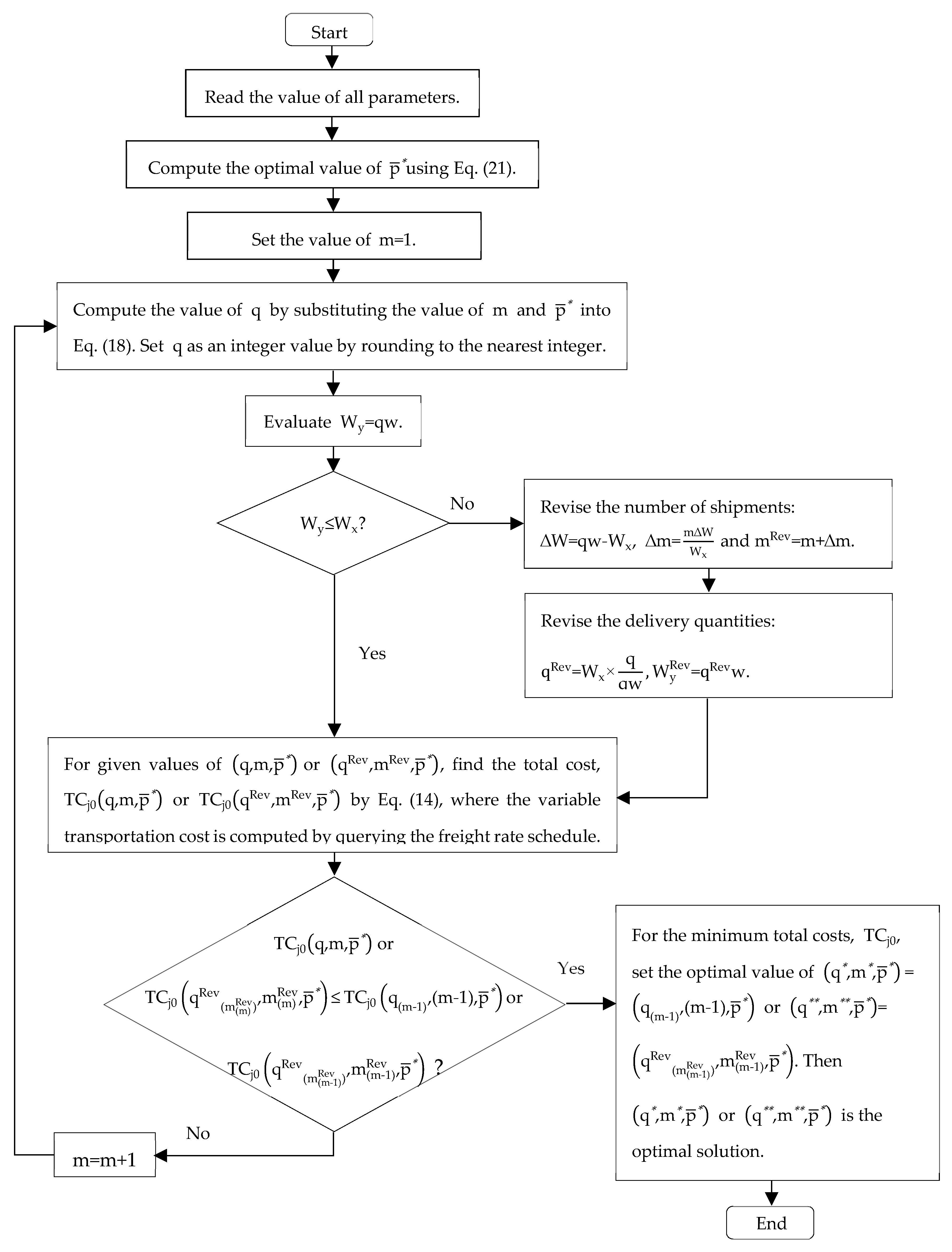However, there is another transportation mode, which is the FTL shipment, which occurs in practice in supply chains [2]. In this case, the delivery quantity based on the FTL shipment is larger than the LTL shipment. Accordingly, an inventory model with an FTL shipment can also result in lower costs, depending on the case. Moreover, there may be other existing solutions that are not restricted to FTL and LTL shipments. To analyse this condition, an enumeration method was proposed to find the best solution for optimizing the performance of supply chains. Hence, the procedure for the enumeration method is presented in Figure 7.

The benefit of enumeration method is used to search for the best solution by evaluating the operation with the least cost through a combination of all the possible solutions. In this case, the objective of the enumeration method is to find out the minimum total cost function with consideration of the actual freight rates. This method was used as a benchmark for comparing the performance with that of the proposed model in terms of the solution quality. Based on Figure 7, the range of solutions for q and m was determined based on the knowledge of the modeller. It was hard to set the size of the solution analytically because this experiment randomly generated scenarios based on the selected parameter.

To gain further insights, the effectiveness of the proposed model was studied by experimenting with a wide range of intervals on the selected parameters. The value of each input parameter was generated randomly to create new scenarios. To undertake this experiment, 1000 problems were randomly generated using the parameter ranges presented in

Table 6. The range of parameters for random generation.

Parameter	Ranges
$\mathrm{D}$	10,000–20,000 units/year
$\mathrm{P}$	10,000–30,000 units/year, $\mathrm{P}>\mathrm{D}$
$\mathrm{A}$	$0–500/order
$\mathrm{S}$	$1–5000/setup
$H_b$	$1–100/(units.year)
$H_v$	$1–1000/(units.year), $H_b>H_v$
$F_0$	$1–100/shipments
$\mathrm{w}$	1–46 lb/unit
$C_n$	$1–50 ($/unit)
$C_m$	$1–50 ($/unit)

. In order to facilitate the computation process, the procedure for the proposed model and the enumeration method was coded using Matlab^® in a DELL inspiron 15 with Intel^® Core™ i3-3227U (1.90 GHz) and 8.00 GB RAM under a 64-bit operating system computer. In the coding process, the procedure for the proposed model and the enumeration method were combined into one. For each problem will be analysed its solution and model performance by using the proposed model and enumeration method. Hence, the best solution and performance of the model for both the proposed model and enumeration method were recorded. However, if the enumeration method was unable to achieve the best solution for one scenario, then, such a scenario was eliminated, and a new scenario was randomly generated. This might mean that the solution for the model was out of the given range.

The results of the experiments on a wide range of parameters are presented in

Table 7. Total problems for each gap range for the best solution.

Gap Range (%)	<0.1	<1	<10	>10
Number of problems	386	508	106	0
Percentage (%)	38.6	50.8	10.6	0
Cumulative problems	38.6	89.4	100	100

. Table 7 shows that the proposed model was technically close to the best solution that could be identified. The gap was divided into various ranges, representing the closeness to the best solution. Tests with the proposed model generated very good results, where 38.6% of all the problems fell within the 0.00–0.1% range, and 50.8% of all the problems were within the 0.1–1.00% range. Moreover, only 10.6% of all the problems were in the range of 1–10%, and none of the problems were above the range of 10%. It can be stated that the proposed model obtained the best results for the 1000 problems mainly due to the fact that most of the problem structures occurred in the gap ranging from 0.00–0.10% to 0.1–1%.

The majority problems show that the proposed model provides near-optimum or optimum inventory decision for minimising system costs. The result shows that cost performance of the proposed model is close to that of best cost performance of enumeration method. Therefore, the solutions of the proposed model can be practically used to solve the problem of transportation and quality. However, since there is gap between the proposed model and enumeration method, this study analysed the gap that occurs due to the solution of proposed model which only works for transportation problem under LTL shipment. It is because the determination of q (see Equation (18)) is added with consideration of transportation function that emulates LTL shipment. Therefore, the optimality level of the proposed model in some cases might result in local optimum solution.

Unlike the proposed model, the enumeration method searches the solutions without being restricted to the mode of LTL shipment. The optimality level of enumeration method in all cases results in global solution. It is due to the enumeration method searching for the optimum condition by combining all possible solutions and then choosing a solution that provides minimum system cost. In this supply chain practice, the solution procedure of enumeration method can be used by the supply chain manager to plan their operations considering transportation and quality problem. Hence, global minimum solution can be obtained in terms of cost performance. The experimentation result shows that the solution of proposed model and enumeration method are recommended for managers to improve the supply chain practices under certain case of transportation and quality.

7. Conclusions

This paper considered an integrated inventory decision-making model by taking into account the transportation cost and quality improvement investment in the JIT vendor-buyer environment. The proposed model was motivated by the implementation of the JIT inventory management system, which is aimed at reducing stock holding costs by frequent deliveries in smaller lot sizes with higher quality products. The proposed model is also developed by the literature studies that was considered into two categories—(i) integrated models with transportation costs and (ii) integrated models with quality improvement. As previous studies have considered each category separately, the contribution of this paper is to recommend a new approach in improving the utilisation of transportation payload and a product’s quality in the process of inventory replenishment. It can be done by finding optimum delivery quantity, production batch, number of shipments, and process quality that can minimise the total system cost of vendor and buyer.

A number of useful insights gained from the proposed model can be summarised as (i) incorporating transportation costs into the integrated inventory model provides useful information such as the strategic decision to include optimal delivery quantity and the number of shipments for utilising the transportation payload when the truckload capacity is large or limited; (ii) the effect of introducing investment in quality improvements can improve the vendor’s production process, where the probability of acceptable products increases and, thereby, the cost for returning and replacing defective products is reduced; (iii) the results of the sensitivity analysis provide a useful insight for assisting managers in handling the critical parameters that affect the solution and the total cost performance; and (iv) the result of comparing the performance of the proposed model with the enumeration method, which had the best solution, and proved that the proposed model can produce promising results and was close to the best solution. Therefore, this integrated model can be more practical and beneficial for JIT practices as a decision-making tool for determining optimal inventory replenishment decisions and thereby reducing total costs to the members of the supply chain.

For future research, some possible extensions could be considered to this model. In term of quality issues, the detail rework operation to improve product quality can be integrated into the model. For transportation issues, it is better to include reverse logistics as a separate cost from the process of replacing defective products. Also, most integrated models assume that the rate of demand, production, and the probability of good products are deterministic. This condition is contrary to today’s business situation, which is highly dynamic. According to Glock [5], it is better to consider dynamic parameters in the integrated model so that this study can be more reflective of the actual system.

References

1. Dong, Y.; Carter, C.R.; Dresner, M. JIT purchasing and performance: an exploratory analysis of buyer and supplier perspectives. J. Oper. Manag. 2001, 19, 471–483. [Google Scholar] [CrossRef]
2. Ab Rahman, M.N.; Leuveano, R.A.C.; bin Jafar, F.A.; Saleh, C.; Deros, B.M.; Mahmood, W.M.F.W.; Mahmood, W.H.W. Incorporating logistic costs into a single vendor-buyer JELS model. Appl. Math. Model. 2016, 40, 1339–1351. [Google Scholar] [CrossRef]
3. Ab Rahman, M.N.; Leuveano, R.A.C.; Bin Jafar, F.A.; Saleh, C. Total Cost Reduction Using a Genetic Algorithm for Multi-Vendor and Single Manufacturer. Int. J. Math. Model. Methods Appl. Sci. 2015, 9, 566–575. [Google Scholar]
4. Goyal, S.K. An integrated inventory model for a single supplier- single customer problem. Int. J. Prod. Res. 1976, 15, 107–111. [Google Scholar] [CrossRef]
5. Glock, C.H. The joint economic lot size problem: A review. Int. J. Prod. Econ. 2012, 135, 671–686. [Google Scholar] [CrossRef]
6. Sucky, E. Inventory management in supply chains: A bargaining problem. Int. J. Prod. Econ. 2005, 93–94, 253–262. [Google Scholar] [CrossRef]
7. Nie, L.; Xu, X.; Zhan, D. Incorporating transportation costs into JIT lot splitting decision for coordinated supply chains. J. Adv. Manuf. Syst. 2006, 5, 111–121. [Google Scholar] [CrossRef]
8. Kim, S.-L.; Ha, D. A JIT lot-splitting model for supply chain management: Enhancing buyer-supplier linkage. Int. J. Prod. Econ. 2003, 86, 1–10. [Google Scholar] [CrossRef]
9. Chen, Z.X.; Sarker, B.R. Multi-vendor integrated procurement-production system under shared transportation and just-in-time delivery system. J. Oper. Res. Soc. 2010, 61, 1654–1666. [Google Scholar] [CrossRef]
10. Hoque, M.A. Synchronization in the single-manufacturer multi-buyer integrated inventory supply chain. Eur. J. Oper. Res. 2008, 188, 811–825. [Google Scholar] [CrossRef]
11. Disney, S.M.; Potter, A.T.; Gardner, B.M. The impact of vendor managed inventory on transport operations. Transp. Res. Part E Logist. Transp. Rev. 2003, 39, 363–380. [Google Scholar] [CrossRef]
12. Swenseth, S.R.; Godfrey, M.R. Incorporating transportation costs into inventory replenishment decisions. Int. J. Prod. Econ. 2002, 77, 113–130. [Google Scholar] [CrossRef]
13. Yusup, M.Z.; Wan Mahmood, W.H.; Salleh, M.R.; Ab Rahman, M.N. The implementation of cleaner production practices from Malaysian manufacturers’ perspectives. J. Clean. Prod. 2015, 108, 659–672. [Google Scholar] [CrossRef]
14. Ismail, A.; Ghani, J.A.; Ab Rahman, M.N.; Deros, B.; Hassan, C.; Haron, C. Application of Lean Six Sigma Tools for Cycle Time Reduction in Manufacturing: Case Study in Biopharmaceutical Industry. 2013. [Google Scholar]
15. Rose, A.N.M.; Deros, B.M.; Ab Rahman, M.N. A Study on Lean Manufacturing Implementation in Malaysian Automotive Component Industry. Int. J. Automot. Mech. Eng. 2013, 8, 1467–1476. [Google Scholar] [CrossRef]
16. Tayyab, M.; Sarkar, B.; Ullah, M. Sustainable Lot Size in a Multistage Lean-Green Manufacturing Process under Uncertainty. Mathematics 2019, 7, 20. [Google Scholar] [CrossRef]
17. Yoo, S.H.; Kim, D.; Park, M. Lot sizing and quality investment with quality cost analyses for imperfect production and inspection processes with commercial return. Int. J. Prod. Econ. 2012, 140, 922–933. [Google Scholar] [CrossRef]
18. Majumder, A.; Guchhait, R.; Sarkar, B. Manufacturing quality improvement and setup cost reduction in a vendor-buyer supply chain model. Eur. J. Ind. Eng. 2017, 11, 588–612. [Google Scholar] [CrossRef]
19. Ertogral, K.; Darwish, M.; Ben-Daya, M. Production and shipment lot sizing in a vendor-buyer supply chain with transportation cost. Eur. J. Oper. Res. 2007, 176, 1592–1606. [Google Scholar] [CrossRef]
20. Mutlu, F.; Çetinkaya, S. An integrated model for stock replenishment and shipment scheduling under common carrier dispatch costs. Transp. Res. Part E Logist. Transp. Rev. 2010, 46, 844–854. [Google Scholar] [CrossRef]
21. Madadi, A.; Kurz, M.E.; Ashayeri, J. Multi-level inventory management decisions with transportation cost consideration. Transp. Res. Part E Logist. Transp. Rev. 2010, 46, 719–734. [Google Scholar] [CrossRef]
22. Lee, S.-D.; Fu, Y.-C. Joint production and shipment lot sizing for a delivery price-based production facility. Int. J. Prod. Res. 2013, 51, 6152–6162. [Google Scholar] [CrossRef]
23. Lee, S.-D.; Fu, Y.C. Joint production and delivery lot sizing for a make-to-order producer-buyer supply chain with transportation cost. Transp. Res. Part E Logist. Transp. Rev. 2014, 66, 23–35. [Google Scholar] [CrossRef]
24. Leuveano, R.A.C.; Bin Jafar, F.A.; Saleh, C.; Bin Muhamad, M.R.; Ab Rahman, M.N. Incorporating Transportation Cost into Joint Economic Lot Size For Single Vendor-Buyer. J. Softw. 2014, 9, 1313–1323. [Google Scholar] [CrossRef]
25. Sarkar, B.; Ganguly, B.; Sarkar, M.; Pareek, S. Effect of variable transportation and carbon emission in a three-echelon supply chain model. Transp. Res. Part E Logist. Transp. Rev. 2016, 91, 112–128. [Google Scholar] [CrossRef]
26. Affisco, J.F.; Paknejad, M.J.; Nasri, F. Quality improvement and setup reduction in the joint economic lot size model. Eur. J. Oper. Res. 2002, 142, 497–508. [Google Scholar] [CrossRef]
27. Liu, X.; Çetinkaya, S. A note on “quality improvement and setup reduction in the joint economic lot size model.”. Eur. J. Oper. Res. 2007, 182, 194–204. [Google Scholar] [CrossRef]
28. Yang, J.-S.; Pan, J.C.-H. Just-in-time purchasing: An integrated inventory model involving deterministic variable lead time and quality improvement investment. Int. J. Prod. Res. 2004, 42, 853–863. [Google Scholar] [CrossRef]
29. Ouyang, L.-Y.; Wu, K.-S.; Ho, C.-H. An integrated vendor-buyer inventory model with quality improvement and lead time reduction. Int. J. Prod. Econ. 2007, 108, 349–358. [Google Scholar] [CrossRef]
30. Sarkar, B.; Majumder, A.; Sarkar, M.; Kim, N.; Ullah, M. Effects of variable production rate on quality of products in a single-vendor multi-buyer supply chain management. Int. J. Adv. Technol. 2018, 99, 567–581. [Google Scholar] [CrossRef]
31. Dey, B.K.; Sarkar, B. A Two-Echelon Supply Chain Management With Setup Time and Cost Reduction, Quality Improvement and Variable Production Rate. Mathematics 2019, 7, 328. [Google Scholar] [CrossRef]
32. Joglekar, P.N. Note—Comments on “A Quantity Discount Pricing Model to Increase Vendor Profits.”. Manag. Sci. 1988, 34, 1391–1398. [Google Scholar] [CrossRef]
33. Arshinder; Kanda, A.; Deshmukh, S.G. Supply chain coordination: Perspectives, empirical studies and research directions. Int. J. Prod. Econ. 2008, 115, 316–335. [Google Scholar] [CrossRef]
34. Bahinipati, B.K.; Kanda, A.; Deshmukh, S.G. Coordinated supply management: review, insights, and limitations. Int. J. Logist. Res. Appl. 2013, 12, 37–41. [Google Scholar] [CrossRef]
35. Kung, K.Y.; Huang, Y.D.; Wee, H.M. Production-Inventory System for Deteriorating Items with Machine Breakdown, Inspection, and Partial Backordering. Mathematics 2019, 7, 616. [Google Scholar] [CrossRef]
36. Sarkar, B.; Ullah, M. Joint Inventory and Pricing Policy for an Online to Offline Closed-Loop Supply Chain Model with Random Defective Rate and Returnable Transport Items. Mathematics 2019, 7, 497. [Google Scholar] [CrossRef]
37. Hishamuddin, H.; Sarker, R.A.; Essam, D. A recovery model for a two-echelon serial supply chain with consideration of transportation disruption. Comput. Ind. Eng. 2013, 64, 552–561. [Google Scholar] [CrossRef]
38. Darom, N.A.; Hishamuddin, H.; Ramli, R.; Nopiah, Z.M. An inventory model of supply chain disruption recovery with safety stock and carbon emission consideration. J. Clean. Prod. 2018, 197, 1011–1021. [Google Scholar] [CrossRef]
39. Hishamuddin, H.; Sarker, R.; Essam, D.; Defence, A.; Academy, F. An inventory recovery model for an economic lot sizing problem with disruption. J. Teknol. 2016, 78, 143–148. [Google Scholar] [CrossRef]
40. Seyedi, I.; Mirzazadeh, S.; Maleki-Daronkolaei, A.; Mukhtar, M.; Sahran, S. An inventory model with reworking and setup time to consider effect of inflation and time value of money. J. Eng. Sci. Technol. 2016, 11, 416–430. [Google Scholar]
41. Darom, N.A.; Hishamuddin, H.; Ramli, R.; Nopiah, Z.M.; Sarker, R.A. An Integrated Vendor-Buyer Model Subject to Supply Disruption with Transportation Cost. J. Mech. Eng. 2018, 7, 241–258. [Google Scholar]
42. Rice, G.E.; Ambrose, R.B. Mercury Study Report to Congress, 1997; Vol. 3.
Figure 1. The flow of material and transaction cost between vendor and buyer.
Mathematics 07 00944 g001
Figure 2. The trajectory of inventory replenishment between vendor and buyer.
Mathematics 07 00944 g002
Figure 3. The solution procedure of the proposed model.
Mathematics 07 00944 g003
Figure 4. Actual freight rate schedules. Note: lb* is constant charge per pound (lb).
Mathematics 07 00944 g004
Figure 5. Effect of the number of shipments on total cost: (a) incapacitated and (b) capacitated.
Mathematics 07 00944 g005
Figure 6. Impact of the parameter S ,   A ,   H b ,   F 0 ,   α ,   F x ,   C n ,   C m , and i to the model solution q * , m * ,   p - * , and T C j 0 .
Mathematics 07 00944 g006
Figure 7. The procedure for the enumeration method.
Mathematics 07 00944 g007