Article

Higher-Order Derivative-Free Iterative Methods for Solving Nonlinear Equations and Their Basins of Attraction

1
Inner Mongolia Vocational College of Chemical Engineering, Hohhot 010070, China
2
Department of Mathematics, Saveetha Engineering College, Chennai 602105, India
*
Authors to whom correspondence should be addressed.
Mathematics 2019, 7(11), 1052; https://doi.org/10.3390/math7111052
Submission received: 8 September 2019 / Revised: 12 October 2019 / Accepted: 16 October 2019 / Published: 4 November 2019
(This article belongs to the Special Issue Iterative Methods for Solving Nonlinear Equations and Systems)

Abstract

:
Based on the Steffensen-type method, we develop fourth-, eighth-, and sixteenth-order algorithms for solving one-variable equations. The new methods are fourth-, eighth-, and sixteenth-order converging and require at each iteration three, four, and five function evaluations, respectively. Therefore, all these algorithms are optimal in the sense of Kung–Traub conjecture; the new schemes have an efficiency index of 1.587, 1.682, and 1.741, respectively. We have given convergence analyses of the proposed methods and also given comparisons with already established known schemes having the same convergence order, demonstrating the efficiency of the present techniques numerically. We also studied basins of attraction to demonstrate their dynamical behavior in the complex plane.

1. Introduction

Finding faster and exact roots of scalar nonlinear equations is the most important problem in engineering, scientific computing, and applied mathematics. In general, this is the problem of solving a nonlinear equation f ( x ) = 0 . Analytical methods for finding solutions of such problems are almost nonavailable, so the only way to get appropriate solutions by numerical methods is based on iterative algorithms. Newton’s method is one of the well-known and famous methods for finding solutions of nonlinear equations or local minima in problems of optimization. Despite its nice properties, it will often not work efficiently in some real-life practical applications. Ill conditioning of the problems, the computational expense of functional derivative, accurate initial guesses, and a late convergence rate generally lead to difficulties in its use. Nevertheless, many advantages in all of these drawbacks have been found and led to efficient algorithms or codes that can be easily used (see References [1,2] and references therein). Hence, Steffensen developed a derivative-free iterative method ( S M 2 ) (see References [3]):
w ( n ) = x ( n ) + f ( x ( n ) ) , x ( n + 1 ) = x ( n ) f ( x ( n ) ) f [ x ( n ) , w ( n ) ] ,
where f [ x ( n ) , w ( n ) ] = f ( x ( n ) ) f ( w ( n ) ) x ( n ) w ( n ) , which preserves the convergence order and efficiency index of Newton’s method.
The main motivation of this work is to implement efficient derivative-free algorithms for finding the solution of nonlinear equations. We obtained an optimal iterative method that will support the conjecture [4]. Kung–Traub conjectured that multipoint iteration methods without memory based on d functional evaluations could achieve an optimal convergence order 2 d 1 . Furthermore, we studied the behavior of iterative schemes in the complex plane.
Let us start a short review of the literature with some of the existing methods with or without memory before proceeding to the proposed idea. Behl et al. [5] presented an optimal scheme that does not need any derivative evaluations. In addition, the given scheme is capable of generating new optimal eighth-order methods from the earlier optimal fourth-order schemes in which the first sub-step employs Steffensen’s or a Steffensen-type method. Salimi et al. [6] proposed a three-point iterative method for solving nonlinear equations. The purpose of this work is to upgrade a fourth-order iterative method by adding one Newton step and by using a proportional approximation for the last derivative. Salimi et al. [7] constructed two optimal Newton–Secant-like iterative methods for finding solutions of nonlinear equations. The classes have convergence orders of four and eight and cost only three and four function evaluations per iteration, respectively. Matthies et al. [8] proposed a three-point iterative method without memory for solving nonlinear equations with one variable. The method provides a convergence order of eight with four function evaluations per iteration. Sharifi et al. [9] presented an iterative method with memory based on the family of King’s methods to solve nonlinear equations. The method has eighth-order convergence and costs only four function evaluations per iteration. An acceleration of the convergence speed is achieved by an appropriate variation of a free parameter in each step. This self-accelerator parameter is estimated using Newton’s interpolation fourth degree polynomial. The order of convergence is increased from eight to 12 without any extra function evaluation. Khdhr et al. [10] suggested a variant of Steffensen’s iterative method with a convergence order of 3.90057 for solving nonlinear equations that are derivative-free and have memory. Soleymani et al. [11] presented derivative-free iterative methods without memory with convergence orders of eight and sixteen for solving nonlinear equations. Soleimani et al. [12] proposed a optimal family of three-step iterative methods with a convergence order of eight by using a weight function alongside an approximation for the first derivative. Soleymani et al. [13] gave a class of four-step iterative schemes for finding solutions of one-variable equations. The produced methods have better order of convergence and efficiency index in comparison with optimal eighth-order methods. Soleymani et al. [14] constructed a class of three-step eighth order iterative methods by using an interpolatory rational function in the third step. Each method of the class reaches the optimal efficiency index according to the Kung–Traub conjecture concerning multipoint iterative methods without memory. Kanwar et al. [15] suggested two new eighth-order classes of Steffensen–King-type methods for finding solutions of nonlinear equations numerically. Cordero et al. [1] proposed a general procedure to obtain derivative-free iterative methods for finding solutions of nonlinear equations by polynomial interpolation. In addition, many authors have worked with these ideas on different iterative schemes [16,17,18,19,20,21,22,23,24], describing the basin of attraction of some well-known iterative scheme. In this work, we developed a novel fourth-order iterative scheme, eighth-order iterative scheme, and sixteenth-order iterative scheme, that are without memory, are derivative-free, and are optimal.
The rest of this paper is ordered as follows. In Section 2, we present the proposed fourth-, eighth-, and sixteenth-order methods that are free from derivatives. Section 3 presents the convergence order of the proposed scheme. In Section 4, we discuss some well-known iterative methods for the numerical and effectiveness comparison of the proposed schemes. In Section 5, we display the performance of proposed methods and other compared algorithms described by problems. The respective graphical fractal pictures obtained from each iteration scheme for test problems are given in Section 6 to show the consistency of the proposed methods. Finally, Section 7 gives concluding remarks.

2. Development of Derivative-Free Scheme

2.1. Optimal Fourth-Order Method

Let us start from Steffensen’s method and explain the procedure to get optimal methods of increasing order. The idea is to compose a Steffensen’s iteration with Newton’s step as follows:
w ( n ) = x ( n ) + f ( x ( n ) ) 3 , y ( n ) = x ( n ) f ( x ( n ) ) 4 f ( w ( n ) ) f ( x ( n ) ) , z ( n ) = y ( n ) f ( y ( n ) ) f ( y ( n ) ) .
The resulting iteration has convergence order four, with the composition of two second-order methods, but the method is not optimal because it uses four function evaluations. In order to get an optimality, we need to reduce a function and to preserve the same convergence order, and so, we estimate f ( y ( n ) ) by the following polynomial:
N 2 ( t ) = f ( y ( n ) ) + ( t y ( n ) ) f [ y ( n ) , w ( n ) ] + ( t y ( n ) ) ( t w ( n ) ) f [ y ( n ) , w ( n ) , x ( n ) ] ,
where
f [ x ( 0 ) , x ( 1 ) , x ( 2 ) , , x ( k 1 ) , x ( k ) ] = f [ x ( 1 ) , x ( 2 ) , , x ( k 1 ) , x ( k ) ] f [ x ( 0 ) , x ( 1 ) , x ( 2 ) , , x ( k 1 ) ] x ( k ) x ( 0 ) , x ( k ) x ( 0 ) ,
is the generalized divided differences of kth order at x ( 0 ) x ( 1 ) x ( 2 ) x ( k 1 ) x ( k ) . It is noted that N 2 ( y ( n ) ) = f ( y ( n ) ) . Differentiating Equation (3) and putting t = y ( n ) , we get
N 2 ( y ( n ) ) = f [ y ( n ) , w ( n ) ] + ( y ( n ) w ( n ) ) f [ y ( n ) , w ( n ) , x ( n ) ] .
Now, approximating f ( y ( n ) ) N 2 ( y ( n ) ) in Equation (2), we get a new derivative-free optimal fourth-order method ( P M 4 ) given by
w ( n ) = x ( n ) + f ( x ( n ) ) 3 , y ( n ) = x ( n ) f ( x ( n ) ) 4 f ( w ( n ) ) f ( x ( n ) ) , z ( n ) = y ( n ) f ( y ( n ) ) f [ y ( n ) , w ( n ) ] + ( y ( n ) w ( n ) ) f [ y ( n ) , w ( n ) , x ( n ) ] .

2.2. Optimal Eighth-Order Method

Next, we attempt to get a new optimal eighth-order method in the following way:
w ( n ) = x ( n ) + f ( x ( n ) ) 3 , y ( n ) = x ( n ) f ( x ( n ) ) 4 f ( w ( n ) ) f ( x ( n ) ) , z ( n ) = y ( n ) f ( y ( n ) ) f [ y ( n ) , w ( n ) ] + ( y ( n ) w ( n ) ) f [ y ( n ) , w ( n ) , x ( n ) ] , p ( n ) = z ( n ) f ( z ( n ) ) f ( z ( n ) ) .
The above has eighth-order convergence with five function evaluations, but this is not an optimal method. To get an optimal, we need to reduce a function and to preserve the same convergence order, and so, we estimate f ( z ( n ) ) by the following polynomial:
N 3 ( t ) = f ( z ( n ) ) + ( t z ( n ) ) f [ z ( n ) , y ( n ) ] + ( t z ( n ) ) ( t y ( n ) ) f [ z ( n ) , y ( n ) , w ( n ) ] + ( t z ( n ) ) ( t y ( n ) ) ( t w ( n ) ) f [ z ( n ) , y ( n ) , w ( n ) , x ( n ) ] .
It is clear that N 3 ( z ( n ) ) = f ( z ( n ) ) . Differentiating Equation (7) and setting t = z ( n ) , we get
N 3 ( z ( n ) ) = f [ z ( n ) , y ( n ) ] + ( z ( n ) y ( n ) ) f [ z ( n ) , y ( n ) , w ( n ) ] + ( z ( n ) y ( n ) ) ( z ( n ) w ( n ) ) f [ z ( n ) , y ( n ) , w ( n ) , x ( n ) ] .
Now, approximating f ( z ( n ) ) N 3 ( z ( n ) ) in (6), we get a new derivative-free optimal eighth-order method ( P M 8 ) given by
w ( n ) = x ( n ) + f ( x ( n ) ) 3 , y ( n ) = x ( n ) f ( x ( n ) ) 4 f ( w ( n ) ) f ( x ( n ) ) , z ( n ) = y ( n ) f ( y ( n ) ) f [ y ( n ) , w ( n ) ] + ( y ( n ) w ( n ) ) f [ y ( n ) , w ( n ) , x ( n ) ] , p ( n ) = z ( n ) f ( z ( n ) ) f [ z ( n ) , y ( n ) ] + ( z ( n ) y ( n ) ) f [ z ( n ) , y ( n ) , w ( n ) ] + ( z ( n ) y ( n ) ) ( z ( n ) w ( n ) ) f [ z ( n ) , y ( n ) , w ( n ) , x ( n ) ] .

2.3. Optimal Sixteenth-Order Method

Next, we attempt to get a new optimal sixteenth-order method in the following way:
w ( n ) = x ( n ) + f ( x ( n ) ) 3 , y ( n ) = x ( n ) f ( x ( n ) ) 4 f ( w ( n ) ) f ( x ( n ) ) , z ( n ) = y ( n ) f ( y ( n ) ) f [ y ( n ) , w ( n ) ] + ( y ( n ) w ( n ) ) f [ y ( n ) , w ( n ) , x ( n ) ] , p ( n ) = z ( n ) f ( z ( n ) ) f [ z ( n ) , y ( n ) ] + ( z ( n ) y ( n ) ) f [ z ( n ) , y ( n ) , w ( n ) ] + ( z ( n ) y ( n ) ) ( z ( n ) w ( n ) ) f [ z ( n ) , y ( n ) , w ( n ) , x ( n ) ] , x ( n + 1 ) = p ( n ) f ( p ( n ) ) f ( p ( n ) ) .
The above has sixteenth-order convergence with six function evaluations, but this is not an optimal method. To get an optimal, we need to reduce a function and to preserve the same convergence order, and so, we estimate f ( p ( n ) ) by the following polynomial:
N 4 ( t ) = f ( p ( n ) ) + ( t p ( n ) ) f [ p ( n ) , z ( n ) ] + ( t p ( n ) ) ( t z ( n ) ) f [ p ( n ) , z ( n ) , y ( n ) ] + ( t p ( n ) ) ( t z ( n ) ) ( t y ( n ) ) f [ p ( n ) , z ( n ) , y ( n ) , w ( n ) ] + ( t p ( n ) ) ( t z ( n ) ) ( t y ( n ) ) ( t w ( n ) ) f [ p ( n ) , z ( n ) , y ( n ) , w ( n ) , x ( n ) ] .
It is clear that N 4 ( p ( n ) ) = f ( p ( n ) ) . Differentiating Equation (11) and setting t = p ( n ) , we get
N 4 ( p ( n ) ) = f [ p ( n ) , z ( n ) ] + ( p ( n ) z ( n ) ) f [ p ( n ) , z ( n ) , y ( n ) ] + ( p ( n ) z ( n ) ) ( p ( n ) y ( n ) ) f [ p ( n ) , z ( n ) , y ( n ) , w ( n ) ] + ( p ( n ) z ( n ) ) ( p ( n ) y ( n ) ) ( p ( n ) w ( n ) ) f [ p ( n ) , z ( n ) , y ( n ) , w ( n ) , x ( n ) ] .
Now, approximating f ( p ( n ) ) N 4 ( p ( n ) ) in Equation (10), we get a new derivative-free optimal sixteenth-order iterative method ( P M 16 ) given by
w ( n ) = x ( n ) + f ( x ( n ) ) 3 , y ( n ) = x ( n ) f ( x ( n ) ) 4 f ( w ( n ) ) f ( x ( n ) ) , z ( n ) = y ( n ) f ( y ( n ) ) f [ y ( n ) , w ( n ) ] + ( y ( n ) w ( n ) ) f [ y ( n ) , w ( n ) , x ( n ) ] , p ( n ) = z ( n ) f ( z ( n ) ) f [ z ( n ) , y ( n ) ] + ( z ( n ) y ( n ) ) f [ z ( n ) , y ( n ) , w ( n ) ] + ( z ( n ) y ( n ) ) ( z ( n ) w ( n ) ) f [ z ( n ) , y ( n ) , w ( n ) , x ( n ) ] , x ( n + 1 ) = p ( n ) f ( p ( n ) ) N 4 ( p ( n ) ) ,
where N 4 ( p ( n ) ) given in Equation (12).

3. Convergence Analysis

In this part, we will derive the convergence analysis of the proposed schemes in Equations (5), (9), and (13) with the help of Mathematica software.
Theorem 1.
Let f : D R R be a sufficiently smooth function having continuous derivatives. If f ( x ) has a simple root x * in the open interval D and x ( 0 ) is chosen in a sufficiently small neighborhood of x * , then the method of Equation (5) is of local fourth-order convergence and and it satisfies the error equation
e n + 1 = ( c [ 2 ] 3 c [ 2 ] c [ 3 ] ) e n 4 + O ( e n 5 ) .
Proof. 
Let e n = x ( n ) x * and c [ j ] = f ( j ) ( x * ) j ! f ( x * ) , j = 2 , 3 , 4 , . Expanding f ( x ( n ) ) and f ( w ( n ) ) about x * by Taylor’s method, we have
f ( x ( n ) ) = f ( x * ) [ e n + c [ 2 ] e n 2 + c [ 3 ] e n 3 + c [ 4 ] e n 4 + ] ,
w ( n ) = e n + f ( x * ) 3 [ e n + c [ 2 ] e n 2 + c [ 3 ] e n 3 + c [ 4 ] e n 4 + ] 3 ,
f ( w ( n ) ) = f ( x * ) [ e n + c [ 2 ] e n 2 + ( f ( x * ) 3 + c [ 3 ] ) e n 3 + ( 5 f ( x * ) 3 c [ 2 ] + c [ 4 ] ) e n 4 + ] .
Then, we have
y ( n ) = x * + c [ 2 ] e n 2 + ( 2 c [ 2 ] 2 + 2 c [ 3 ] ) e n 3 + ( 4 c [ 2 ] 3 7 c [ 2 ] c [ 3 ] + 3 c [ 4 ] + f ( x * ) 3 c [ 2 ] ) e n 4 + .
Expanding f ( y ( n ) ) about x * , we have
f ( y ( n ) ) = f ( x * ) [ c [ 2 ] e n 2 2 ( c [ 2 ] 2 c [ 3 ] ) e n 3 + ( 5 c [ 2 ] 3 7 c [ 2 ] c [ 3 ] + 3 c [ 4 ] + f ( x * ) 3 c [ 2 ] ) e n 4 + ] .
Now, we get the Taylor’s expansion of f [ y ( n ) , w ( n ) ] = f ( y ( n ) ) f ( w ( n ) ) y ( n ) w ( n ) by replacing Equation (15)–(18).
f [ y ( n ) , w ( n ) ] = f ( x * ) [ 1 + c [ 2 ] e n + ( c [ 2 ] 2 + c [ 3 ] ) e n 2 + ( f ( x * ) 3 c [ 2 ] 2 c [ 2 ] 3 + c [ 2 ] c [ 3 ] + c [ 4 ] ) e n 3 + ] .
Also, we have
f [ y ( n ) , w ( n ) , x ( n ) ] = f ( x * ) [ c [ 2 ] + 2 c [ 3 ] e n + ( c [ 2 ] c [ 3 ] + c [ 4 ] ) e n 2 + ]
Using Equations (14)–(20) in the scheme of Equation (5), we obtain the following error equation:
e n + 1 = ( c [ 2 ] 3 c [ 2 ] c [ 3 ] ) e n 4 + .
This reveals that the proposed method P M 4 attains fourth-order convergence. □
Theorem 2.
Let f : D R R be a sufficiently smooth function having continuous derivatives. If f ( x ) has a simple root x * in the open interval D and x ( 0 ) is chosen in a sufficiently small neighborhood of x * , then the method of Equation (9) is of local eighth-order convergence and and it satisfies the error equation
e n + 1 = c [ 2 ] 2 ( c [ 2 ] 2 c [ 3 ] ) ( c [ 2 ] 3 c [ 2 ] c [ 3 ] + c [ 4 ] ) e n 8 + O ( e n 9 ) .
Theorem 3.
Let f : D R R be a sufficiently smooth function having continuous derivatives. If f ( x ) has a simple root x * in the open interval D and x ( 0 ) is chosen in a sufficiently small neighborhood of x * , then the method of Equation (13) is of local sixteenth-order convergence and and it satisfies the error equation
e n + 1 = c [ 2 ] 4 c [ 2 ] 2 c [ 3 ] 2 c [ 2 ] 3 c [ 2 ] c [ 3 ] + c [ 4 ] c [ 2 ] 4 c [ 2 ] 2 c [ 3 ] + c [ 2 ] c [ 4 ] c [ 5 ] e n 16 + O ( e n 17 ) .

4. Some Known Derivative-Free Methods

Let us consider the following schemes for the purpose of comparison. Derivative-free Kung–Traub’s two-step method (KTM4) [4] is as follows:
y ( n ) = x ( n ) f ( x ( n ) ) f [ x ( n ) , w ( n ) ] , w ( n ) = x ( n ) + f ( x ( n ) ) , x ( n + 1 ) = y ( n ) f ( y ( n ) ) f ( w ( n ) ) [ f ( w ( n ) ) f ( y ( n ) ) ] f [ x ( n ) , y ( n ) ] .
Derivative-free Argyros et al. two-step method (AKKB4) [25] is as follows:
y ( n ) = x ( n ) f ( x ( n ) ) f [ x ( n ) , w ( n ) ] , w ( n ) = x ( n ) + f ( x ( n ) ) , x ( n + 1 ) = y ( n ) f ( y ( n ) ) [ f ( x ( n ) ) 2 f ( y ( n ) ) ] f ( x ( n ) ) f [ y ( n ) , w ( n ) ] 1 f ( y ( n ) ) f ( x ( n ) ) .
Derivative-free Zheng et al. two-step method (ZLM4) [26] is as follows:
y ( n ) = x ( n ) f ( x ( n ) ) f [ x ( n ) , w ( n ) ] , w ( n ) = x ( n ) + f ( x ( n ) ) , x ( n + 1 ) = y ( n ) f ( y ( n ) ) f [ x ( n ) , y ( n ) ] + ( y ( n ) x ( n ) ) f [ x ( n ) , w ( n ) , y ( n ) ] .
Derivative-free Argyros et al. three-step method (AKKB8) [25] is as follows:
y ( n ) = x ( n ) f ( x ( n ) ) f [ x ( n ) , w ( n ) ] , w ( n ) = x ( n ) + f ( x ( n ) ) , z ( n ) = y ( n ) f ( y ( n ) ) [ f ( x ( n ) ) 2 f ( y ( n ) ) ] f ( x ( n ) ) f [ y ( n ) , w ( n ) ] 1 f ( y ( n ) ) f ( x ( n ) ) , x ( n + 1 ) = z ( n ) f ( z ( n ) ) f [ z ( n ) , y ( n ) ] + ( z ( n ) y ( n ) ) f [ z ( n ) , y ( n ) , x ( n ) ] + ( z ( n ) y ( n ) ) ( z ( n ) x ( n ) ) f [ z ( n ) , y ( n ) , x ( n ) , w ( n ) ] .
Derivative-free Kanwar et al. three-step method (KBK8) [15] is as follows:
y ( n ) = x ( n ) f ( x ( n ) ) f [ x ( n ) , w ( n ) ] , w ( n ) = x ( n ) + f ( x ( n ) ) 3 , z ( n ) = y ( n ) f ( y ( n ) ) 2 f [ y ( n ) , x ( n ) ] f [ x ( n ) , w ( n ) ] , x ( n + 1 ) = z ( n ) f ( z ( n ) ) f [ y ( n ) , z ( n ) ] + f [ w ( n ) , y ( n ) , z ( n ) ] ( z ( n ) y ( n ) ) 1 f ( y ( n ) ) f ( x ( n ) ) 3 8 f ( y ( n ) ) f ( z ( n ) ) f ( x ( n ) ) 2 + f ( z ( n ) ) f ( x ( n ) ) + 5 f ( z ( n ) ) f ( y ( n ) ) 2 .
Derivative-free Soleymani three-step method (SM8) [2] is as follows:
w ( n ) = x ( n ) + f ( x ( n ) ) , y ( n ) = x ( n ) f ( x ( n ) ) f [ x ( n ) , w ( n ) ] , z ( n ) = y ( n ) f ( y ( n ) ) f [ x ( n ) , w ( n ) ] ϕ n , x ( n + 1 ) = z ( n ) f ( z ( n ) ) f [ x ( n ) , w ( n ) ] ϕ n ψ n , w h e r e ϕ n = 1 1 f ( y ( n ) ) / f ( x ( n ) ) f ( y ( n ) ) / f ( w ( n ) ) , ψ n = 1 + 1 1 + f [ x ( n ) , w ( n ) ] f ( y ( n ) ) f ( x ( n ) ) 2 + ( 1 + f [ x ( n ) , w ( n ) ] ) ( 2 + f [ x ( n ) , w ( n ) ] ) f ( y ( n ) ) f ( w ( n ) ) 3 + f ( z ( n ) ) f ( y ( n ) ) + f ( z ( n ) ) f ( x ( n ) ) + f ( z ( n ) ) f ( w ( n ) ) .
Derivative-free Zheng et al. four-step method (ZLM16) [26] is as follows:
y ( n ) = x ( n ) f ( x ( n ) ) 2 f ( w ( n ) ) f ( x ( n ) ) , w ( n ) = x ( n ) + f ( x ( n ) ) , z ( n ) = y ( n ) f ( y ( n ) ) f [ y ( n ) , w ( n ) ] + ( y ( n ) w ( n ) ) f [ y ( n ) , w ( n ) , x ( n ) ] , p ( n ) = z ( n ) f ( z ( n ) ) f [ z ( n ) , y ( n ) ] + ( z ( n ) y ( n ) ) f [ z ( n ) , y ( n ) , w ( n ) ] + ( z ( n ) y ( n ) ) ( z ( n ) w ( n ) ) f [ z ( n ) , y ( n ) , w ( n ) , x ( n ) ] , x ( n + 1 ) = p ( n ) f ( p ( n ) ) f ( p ( n ) ) , w h e r e f ( p ( n ) ) f [ p ( n ) , z ( n ) ] + ( p ( n ) z ( n ) ) f [ p ( n ) , z ( n ) , y ( n ) ] + ( p ( n ) z ( n ) ) ( p ( n ) y ( n ) ) f [ p ( n ) , z ( n ) , y ( n ) , w ( n ) ] + ( p ( n ) z ( n ) ) ( p ( n ) y ( n ) ) ( p ( n ) w ( n ) ) f [ p ( n ) , z ( n ) , y ( n ) , w ( n ) , x ( n ) ] .

5. Test Problems

We compare the performance of the proposed methods along with some existing methods for test problems by using Matlab. We use the conditions for stopping criteria for | f ( x ( N ) ) | < ϵ where ϵ = 10 50 and N is the number of iterations needed for convergence. The computational order of convergence ( c o c ) is given by
ρ = ln | ( x ( N ) x ( N 1 ) ) / ( x ( N 1 ) x ( N 2 ) ) | ln | ( x ( N 1 ) x ( N 2 ) ) / ( x ( N 2 ) x ( N 3 ) ) | .
The test problems and their roots are given below:
f 1 ( x ) = sin ( 2 cos x ) 1 x 2 + e sin ( x 3 ) , x * = 0.7848959876612125352 f 2 ( x ) = x 3 + 4 x 2 10 , x * = 1.3652300134140968457 f 3 ( x ) = x 2 + 2 x + 5 2 sin x x 2 + 3 , x * = 2.3319676558839640103 f 4 ( x ) = e x sin x + log ( 1 + x 2 ) 2 , x * = 2.4477482864524245021 f 5 ( x ) = s i n ( x ) + c o s ( x ) + x , x * = 0.4566247045676308244
Table 1, Table 2, Table 3, Table 4 and Table 5 show the results of all the test functions with a given initial point. The computational order of convergence conforms with theoretical order of convergence. If the initial points are close to the zero, then we obtain less number of iterations with least error. If the initial points are away from the zero, then we will not obtained the least error. We observe that the new methods in all the test function have better efficiency as compared to other existing methods of the equivalent methods.

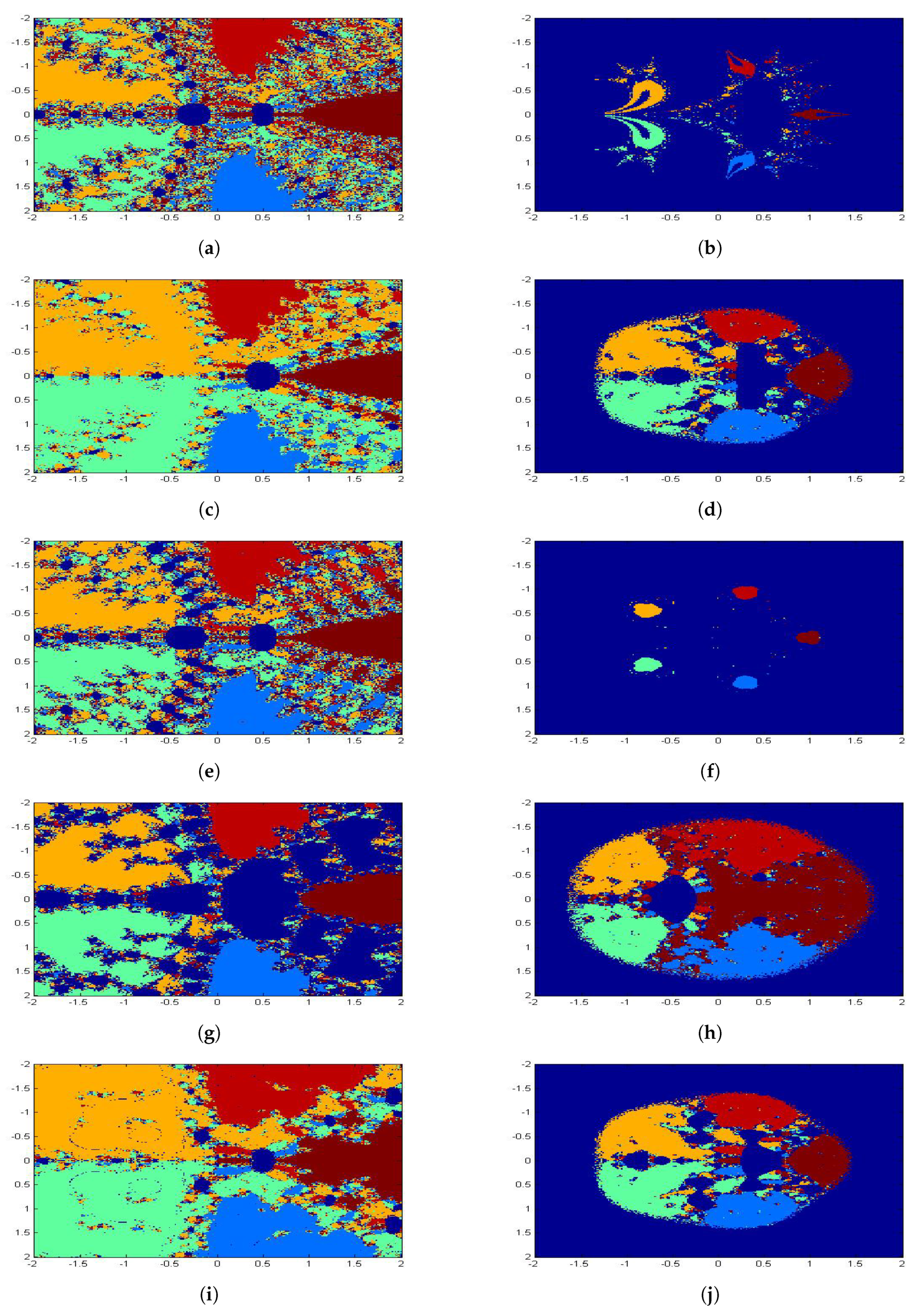
6. Basins of Attraction

The iterative scheme gives information about convergence and stability by studying basins of attraction of the rational function. The basic definitions and dynamical concepts of rational function can found in References [17,27,28]. Let us consider a region R × R = [ 2 , 2 ] × [ 2 , 2 ] with 256 × 256 grids. We test iterative methods in all the grid point z ( 0 ) in the square. The iterative algorithms attempt roots z j * of the equation with condition | f ( z ( k ) ) | < × 10 4 and a maximum of 100 iterations; we conclude that z ( 0 ) is in the basin of attraction of this zero. If the iterative method starting in z ( 0 ) reaches a zero in N iterations, then we mark this point z ( 0 ) with colors if | z ( N ) z j * | < × 10 4 . If N > 50 , then we assign a dark blue color for diverging grid points. We describe the basins of attraction for finding complex roots of p 1 ( z ) = z 2 1 , p 2 ( z ) = z 3 1 , p 3 ( z ) = ( z 2 + 1 ) ( z 2 1 ) , and p 4 ( z ) = z 5 1 for proposed methods and some higher-order iterative methods.
In Figure 1, Figure 2, Figure 3, Figure 4 and Figure 5, we have given the basins of attraction for new methods with some existing methods. We confirm that a point z 0 containing the Julia set whenever the dynamics of point shows sensitivity to the conditions. The neighbourhood of initial points leads to the slight variation in behavior after some iterations. Therefore, some of the compared algorithms obtain more divergent initial conditions.

7. Concluding Remarks

We have proposed fourth-, eighth-, and sixteenth-order methods using finite difference approximations. Our proposed new methods requires 3 functions to get the 4th-order method, 4 functions to obtain the 8th-order method, and 5 functions to get the 16th-order one. We have increased the convergence order of the proposed method, respectively, to four, eight, and sixteen with efficiency indices 1.587, 1.565, and 1.644 respectively. Our new proposed schemes are better than the Steffensen method in terms of efficiency index (1.414). Numerical solutions are tested to show the performance of the proposed algorithms. Also, we have analyzed on the complex region for iterative methods to study their basins of attraction. Hence, we conclude that the proposed methods are comparable to other well-known existing equivalent methods.

Author Contributions

Conceptualization, K.M.; Funding acquisition, J.L. and X.W.; Methodology, K.M.; Project administration, J.L. and X.W.; Resources, J.L. and X.W.; Writing—original draft, K.M.

Funding

This research received no external funding.

Acknowledgments

The authors would like to thank the editors and referees for the valuable comments and for the suggestions to improve the readability of the paper.

Conflicts of Interest

The authors declare no conflict of interest.

References

  1. Cordero, A.; Hueso, J.L.; Martinez, E.; Torregrosa, J.R. Generating optimal derivative free iterative methods for nonlinear equations by using polynomial interpolation. Appl. Math. Comp. 2013, 57, 1950–1956. [Google Scholar] [CrossRef]
  2. Soleymani, F. Efficient optimal eighth-order derivative-free methods for nonlinear equations. Jpn. J. Ind. Appl. Math. 2013, 30, 287–306. [Google Scholar] [CrossRef]
  3. Steffensen, J.F. Remarks on iteration. Scand. Aktuarietidskr. 1933, 16, 64–72. [Google Scholar] [CrossRef]
  4. Kung, H.; Traub, J. Optimal order of one-point and multi-point iteration. J. Assoc. Comput. Math. 1974, 21, 643–651. [Google Scholar] [CrossRef]
  5. Behl, R.; Salimi, M.; Ferrara, M.; Sharifi, S.; Alharbi, S.K. Some Real-Life Applications of a Newly Constructed Derivative Free Iterative Scheme. Symmetry 2019, 11, 239. [Google Scholar] [CrossRef]
  6. Salimi, M.; Long, N.M.A.N.; Sharifi, S.; Pansera, B.A. A multi-point iterative method for solving nonlinear equations with optimal order of convergence. Jpn. J. Ind. Appl. Math. 2018, 35, 497–509. [Google Scholar] [CrossRef]
  7. Salimi, M.; Lotfi, T.; Sharifi, S.; Siegmund, S. Optimal Newton-Secant like methods without memory for solving nonlinear equations with its dynamics. Int. J. Comput. Math. 2017, 94, 1759–1777. [Google Scholar] [CrossRef]
  8. Matthies, G.; Salimi, M.; Sharifi, S.; Varona, J.L. An optimal three-point eighth-order iterative method without memory for solving nonlinear equations with its dynamics. Jpn. J. Ind. Appl. Math. 2016, 33, 751–766. [Google Scholar] [CrossRef] [Green Version]
  9. Sharifi, S.; Siegmund, S.; Salimi, M. Solving nonlinear equations by a derivative-free form of the King’s family with memory. Calcolo 2016, 53, 201–215. [Google Scholar] [CrossRef]
  10. Khdhr, F.W.; Saeed, R.K.; Soleymani, F. Improving the Computational Efficiency of a Variant of Steffensen’s Method for Nonlinear Equations. Mathematics 2019, 7, 306. [Google Scholar] [CrossRef]
  11. Soleymani, F.; Babajee, D.K.R.; Shateyi, S.; Motsa, S.S. Construction of Optimal Derivative-Free Techniques without Memory. J. Appl. Math. 2012, 2012, 24. [Google Scholar] [CrossRef]
  12. Soleimani, F.; Soleymani, F.; Shateyi, S. Some Iterative Methods Free from Derivatives and Their Basins of Attraction for Nonlinear Equations. Discret. Dyn. Nat. Soc. 2013, 2013, 10. [Google Scholar] [CrossRef]
  13. Soleymani, F.; Sharifi, M. On a General Efficient Class of Four-Step Root-Finding Methods. Int. J. Math. Comp. Simul. 2011, 5, 181–189. [Google Scholar]
  14. Soleymani, F.; Vanani, S.K.; Paghaleh, M.J. A Class of Three-Step Derivative-Free Root Solvers with Optimal Convergence Order. J. Appl. Math. 2012, 2012, 15. [Google Scholar] [CrossRef]
  15. Kanwar, V.; Bala, R.; Kansal, M. Some new weighted eighth-order variants of Steffensen-King’s type family for solving nonlinear equations and its dynamics. SeMA J. 2016. [Google Scholar] [CrossRef]
  16. Amat, S.; Busquier, S.; Plaza, S. Dynamics of a family of third-order iterative methods that do not require using second derivatives. Appl. Math. Comput. 2004, 154, 735–746. [Google Scholar] [CrossRef]
  17. Amat, S.; Busquier, S.; Plaza, S. Review of some iterative root-finding methods from a dynamical point of view. SCIENTIA Ser. A Math. Sci. 2004, 10, 3–35. [Google Scholar]
  18. Babajee, D.K.R.; Madhu, K. Comparing two techniques for developing higher order two-point iterative methods for solving quadratic equations. SeMA J. 2019, 76, 227–248. [Google Scholar] [CrossRef]
  19. Cordero, A.; Hueso, J.L.; Martinez, E.; Torregrosa, J.R. A family of iterative methods with sixth and seventh order convergence for nonlinear equations. Math. Comput. Model. 2010, 52, 1490–1496. [Google Scholar] [CrossRef]
  20. Curry, J.H.; Garnett, L.; Sullivan, D. On the iteration of a rational function: computer experiments with Newton’s method. Commun. Math. Phys. 1983, 91, 267–277. [Google Scholar] [CrossRef]
  21. Soleymani, F.; Babajee, D.K.R.; Sharifi, M. Modified Jarratt Method without Memory with Twelfth-Order Convergence. Ann. Univ. Craiova Math. Comput. Sci. Ser. 2012, 39, 21–34. [Google Scholar]
  22. Tao, Y.; Madhu, K. Optimal Fourth, Eighth and Sixteenth Order Methods by Using Divided Difference Techniques and Their Basins of Attraction and Its Application. Mathematics 2019, 7, 322. [Google Scholar] [CrossRef]
  23. Vrscay, E.R. Julia sets and mandelbrot-like sets associated with higher order Schroder rational iteration functions: a computer assisted study. Math. Comput. 1986, 46, 151–169. [Google Scholar]
  24. Vrscay, E.R.; Gilbert, W.J. Extraneous fxed points, basin boundaries and chaotic dynamics for Schroder and Konig rational iteration functions. Numer. Math. 1987, 52, 1–16. [Google Scholar] [CrossRef]
  25. Argyros, I.K.; Kansal, M.; Kanwar, V.; Bajaj, S. Higher-order derivative-free families of Chebyshev-Halley type methods with or without memory for solving nonlinear equations. Appl. Math. Comput. 2017, 315, 224–245. [Google Scholar] [CrossRef]
  26. Zheng, Q.; Li, J.; Huang, F. An optimal Steffensen-type family for solving nonlinear equations. Appl. Math. Comput. 2011, 217, 9592–9597. [Google Scholar] [CrossRef]
  27. Madhu, K. Some New Higher Order Multi-Point Iterative Methods and Their Applications to Differential and Integral Equation and Global Positioning System. Ph.D. Thesis, Pndicherry University, Pondicherry, India, June 2016. [Google Scholar]
  28. Scott, M.; Neta, B.; Chun, C. Basin attractors for various methods. Appl. Math. Comput. 2011, 218, 2584–2599. [Google Scholar] [CrossRef]
Figure 1. Basins of attraction for S M 2 for the polynomial.
Mathematics 07 01052 g001
Figure 2. Polynomiographs of p 1 ( z ) : (a) K T M 4 ; (b) A K K B 4 ; (c) Z L M 4 ; (d) P M 4 ; (e) A K K B 8 ; (f) K B K 8 ; (g) S M 8 ; (h) P M 8 ; (i) Z L M 16 ; and (j) P M 16 .
Mathematics 07 01052 g002
Figure 3. Polynomiographs of p 2 ( z ) : (a) K T M 4 ; (b) A K K B 4 ; (c) Z L M 4 ; (d) P M 4 ; (e) A K K B 8 ; (f) K B K 8 ; (g) S M 8 ; (h) P M 8 ; (i) Z L M 16 ; and (j) P M 16 .
Mathematics 07 01052 g003
Figure 4. Polynomiographs of p 3 ( z ) : (a) K T M 4 ; (b) A K K B 4 ; (c) Z L M 4 ; (d) P M 4 ; (e) A K K B 8 ; (f) K B K 8 ; (g) S M 8 ; (h) P M 8 ; (i) Z L M 16 ; and (j) P M 16 .
Mathematics 07 01052 g004
Figure 5. Polynomiographs of p 4 ( z ) : (a) K T M 4 ; (b) A K K B 4 ; (c) Z L M 4 ; (d) P M 4 ; (e) A K K B 8 ; (f) K B K 8 ; (g) S M 8 ; (h) P M 8 ; (i) Z L M 16 ; and (j) P M 16 .
Mathematics 07 01052 g005
Table 1. Comparisons between different methods for f 1 ( x ) at x ( 0 ) = 0.9 .
MethodsN | x ( 1 ) x ( 0 ) | | x ( 2 ) x ( 1 ) | | x ( 3 ) x ( 2 ) | | x ( N ) x ( N 1 ) | coc
S M 2 (1)80.09960.01496.1109 × 10 4 1.0372 × 10 89 1.99
K T M 4 (22)50.11446.7948 × 10 4 3.4668 × 10 12 5.1591 × 10 178 4.00
A K K B 4 (23)40.11473.6299 × 10 4 9.5806 × 10 14 4.6824 × 10 52 3.99
Z L M 4 (24)50.11456.1744 × 10 4 1.5392 × 10 12 1.3561 × 10 184 4.00
P M 4 (5)40.11501.3758 × 10 4 2.6164 × 10 16 3.4237 × 10 63 3.99
A K K B 8 (25)30.11511.2852 × 10 8 3.7394 × 10 62 3.7394 × 10 62 7.70
K B K 8 (26)30.11518.1491 × 10 8 1.5121 × 10 56 1.5121 × 10 56 7.92
S M 8 (27)40.11511.8511 × 10 6 1.0266 × 10 43 07.99
P M 8 (9)30.11517.1154 × 10 9 9.3865 × 10 67 9.3865 × 10 67 8.02
Z L M 16 (28)30.11515.6508 × 10 15 1.4548 × 10 225 1.4548 × 10 225 15.82
P M 16 (13)30.11515.3284 × 10 17 1.2610 × 10 262 1.2610 × 10 262 16.01
Table 2. Comparisons between different methods for f 2 ( x ) at x ( 0 ) = 1.6 .
MethodsN | x ( 1 ) x ( 0 ) | | x ( 2 ) x ( 1 ) | | x ( 3 ) x ( 2 ) | | x ( N ) x ( N 1 ) | coc
S M 2 (1)120.05600.05580.05201.7507 × 10 83 1.99
K T M 4 (22)50.21840.01633.4822 × 10 6 4.7027 × 10 79 3.99
A K K B 4 (23)330.03360.02680.01712.4368 × 10 52 0.99
Z L M 4 (24)50.22300.01174.4907 × 10 7 3.9499 × 10 95 3.99
P M 4 (5)50.21230.02242.3433 × 10 7 4.3969 × 10 112 4.00
A K K B 8 (25)40.21750.01731.2720 × 10 9 1.0905 × 10 66 8.00
K B K 8 (26)DDDDDD
S M 8 (27)40.23444.1548 × 10 4 9.5789 × 10 24 7.7650 × 10 181 7.89
P M 8 (9)40.23452.4307 × 10 4 4.6428 × 10 32 8.2233 × 10 254 8.00
Z L M 16 (28)30.23482.2048 × 10 7 1.9633 × 10 124 1.9633 × 10 124 15.57
P M 16 (13)30.23482.8960 × 10 8 1.7409 × 10 126 1.7409 × 10 126 17.11
Table 3. Comparisons between different methods for f 3 ( x ) at x ( 0 ) = 2.7 .
MethodsN | x ( 1 ) x ( 0 ) | | x ( 2 ) x ( 1 ) | | x ( 3 ) x ( 2 ) | | x ( N ) x ( N 1 ) | coc
S M 2 (1)70.38610.01804.6738 × 10 05 1.0220 × 10 82 1.99
K T M 4 (22)40.36832.8791 × 10 4 1.0873 × 10 16 2.2112 × 10 66 3.99
A K K B 4 (23)40.36832.5241 × 10 4 5.2544 × 10 17 9.8687 × 10 68 3.99
Z L M 4 (24)40.36833.1466 × 10 4 1.7488 × 10 16 1.6686 × 10 65 4.00
P M 4 (5)40.36832.2816 × 10 4 2.3732 × 10 17 2.7789 × 10 69 3.99
A K K B 8 (25)30.36801.7343 × 10 8 3.8447 × 10 67 3.8447 × 10 67 8.00
K B K 8 (26)40.36804.2864 × 10 5 1.8700 × 10 38 2.4555 × 10 305 7.99
S M 8 (27)30.36807.8469 × 10 8 2.9581 × 10 61 2.9581 × 10 61 8.00
P M 8 (9)30.36809.7434 × 10 9 1.0977 × 10 69 1.0977 × 10 69 8.04
Z L M 16 (28)30.36801.4143 × 10 16 6.3422 × 10 240 6.3422 × 10 240 16.03
P M 16 (13)30.36803.6568 × 10 17 7.4439 × 10 274 7.4439 × 10 274 16.04
Table 4. Comparisons between different methods for f 4 ( x ) at x ( 0 ) = 1.9 .
MethodsN | x ( 1 ) x ( 0 ) | | x ( 2 ) x ( 1 ) | | x ( 3 ) x ( 2 ) | | x ( N ) x ( N 1 ) | coc
S M 2 (1)70.49750.05002.5378 × 10 4 1.9405 × 10 73 2.00
K T M 4 (22)40.25221.7586 × 10 6 1.5651 × 10 26 9.8198 × 10 107 3.99
A K K B 4 (23)40.54890.00113.8305 × 10 15 5.5011 × 10 61 3.99
Z L M 4 (24)40.54879.0366 × 10 4 1.4751 × 10 15 1.0504 × 10 62 3.99
P M 4 (5)40.54813.0864 × 10 4 8.0745 × 10 18 3.7852 × 10 72 3.99
A K K B 8 (25)30.54775.4938 × 10 7 4.9628 × 10 56 4.9628 × 10 56 8.17
K B K 8 (26)30.54774.1748 × 10 7 5.8518 × 10 59 5.8518 × 10 59 8.47
S M 8 (27)30.54775.4298 × 10 7 4.1081 × 10 56 4.1081 × 10 56 8.18
P M 8 (9)30.54775.8222 × 10 8 1.1144 × 10 64 1.1144 × 10 64 8.13
Z L M 16 (28)30.54772.7363 × 10 14 7.2982 × 10 229 7.2982 × 10 229 16.13
P M 16 (13)30.54775.6240 × 10 16 1.9216 × 10 257 1.9216 × 10 257 16.11
Table 5. Comparisons between different methods for f 5 ( x ) at x ( 0 ) = 0.2 .
MethodsN | x ( 1 ) x ( 0 ) | | x ( 2 ) x ( 1 ) | | x ( 3 ) x ( 2 ) | | x ( N ) x ( N 1 ) | coc
S M 2 (1)70.30720.04996.4255 × 10 4 4.1197 × 10 59 2.00
K T M 4 (22)50.25850.00191.5538 × 10 12 3.4601 × 10 194 4.00
A K K B 4 (23)40.25714.4142 × 10 4 3.4097 × 10 15 1.2154 × 10 59 3.99
Z L M 4 (24)40.25800.00133.5840 × 10 13 1.8839 × 10 51 3.99
P M 4 (5)40.25692.8004 × 10 4 6.2960 × 10 17 1.6097 × 10 67 3.99
A K K B 8 (25)30.25664.1915 × 10 8 6.3444 × 10 65 6.3444 × 10 65 8.37
K B K 8 (26)40.25664.0069 × 10 6 5.1459 × 10 47 07.99
S M 8 (27)40.25662.9339 × 10 6 1.0924 × 10 46 07.99
P M 8 (9)30.25663.7923 × 10 11 9.0207 × 10 90 9.0207 × 10 90 7.99
Z L M 16 (28)30.25665.3695 × 10 16 7.0920 × 10 252 7.0920 × 10 252 16.06
P M 16 (13)30.25661.1732 × 10 19 1.2394 × 10 314 1.2394 × 10 314 16.08

