An Estimate of the Root Mean Square Error Incurred When Approximating an f ∈ L2(ℝ) by a Partial Sum of Its Hermite Series


Abstract
:1. Introduction
2. Approximation Using the Dirichlet Operator
3. The Sansone Estimates
3.1. Estimate of
3.2. Estimate of
3.3. Estimate for
3.4. Estimate of
3.5. Estimate of
- (i)
- The termis no bigger than:in which:
- (ii)
- Arguing as in (i), we have:
- (iii)
- The mean square on of:is dominated by:
- (iv)
- The method of (ii) applied to the estimation of the square mean on , of:leads to the upper bound:
- (v)
- The square mean, on , of:is, by a now familiar argument,
4. The Proof of Theorem 1
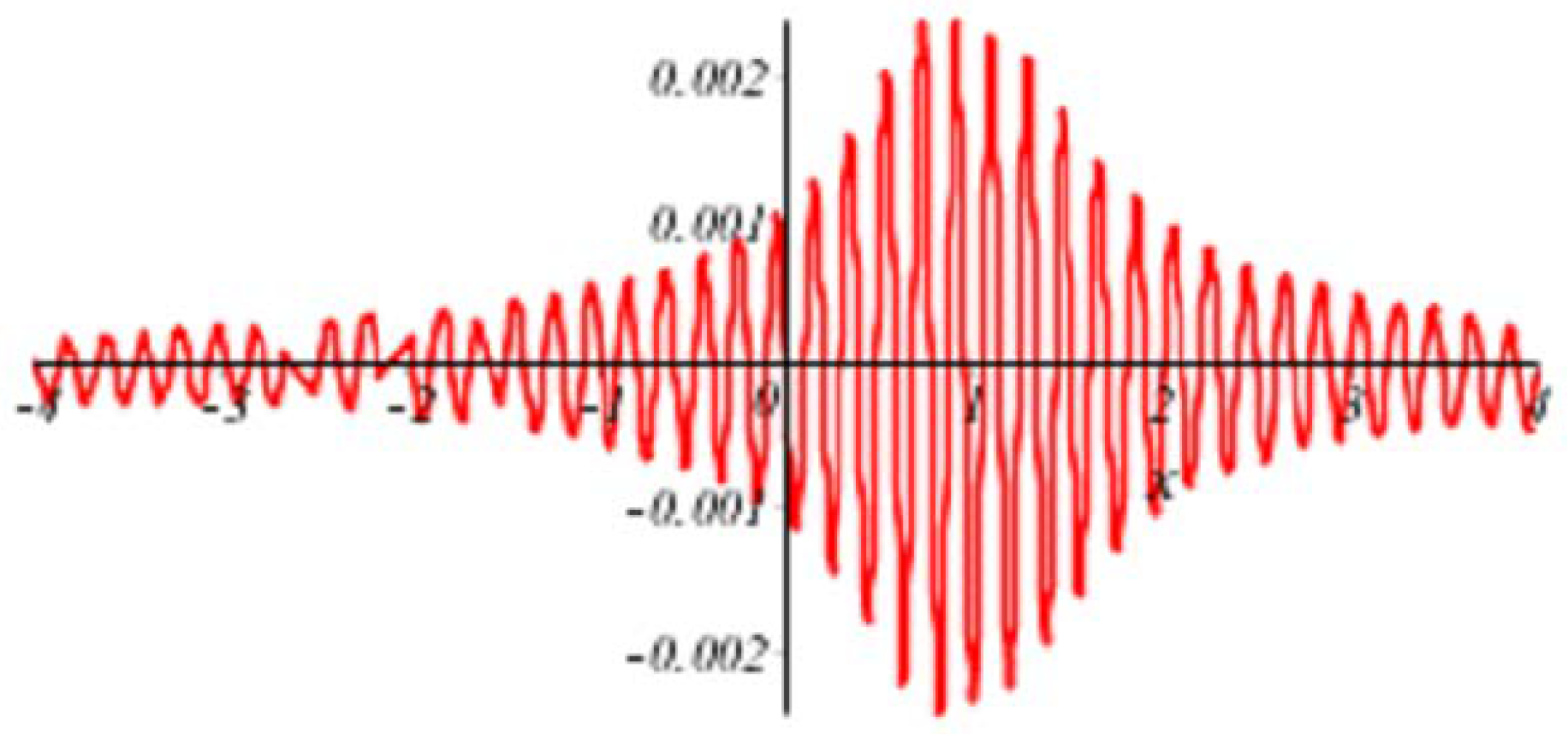
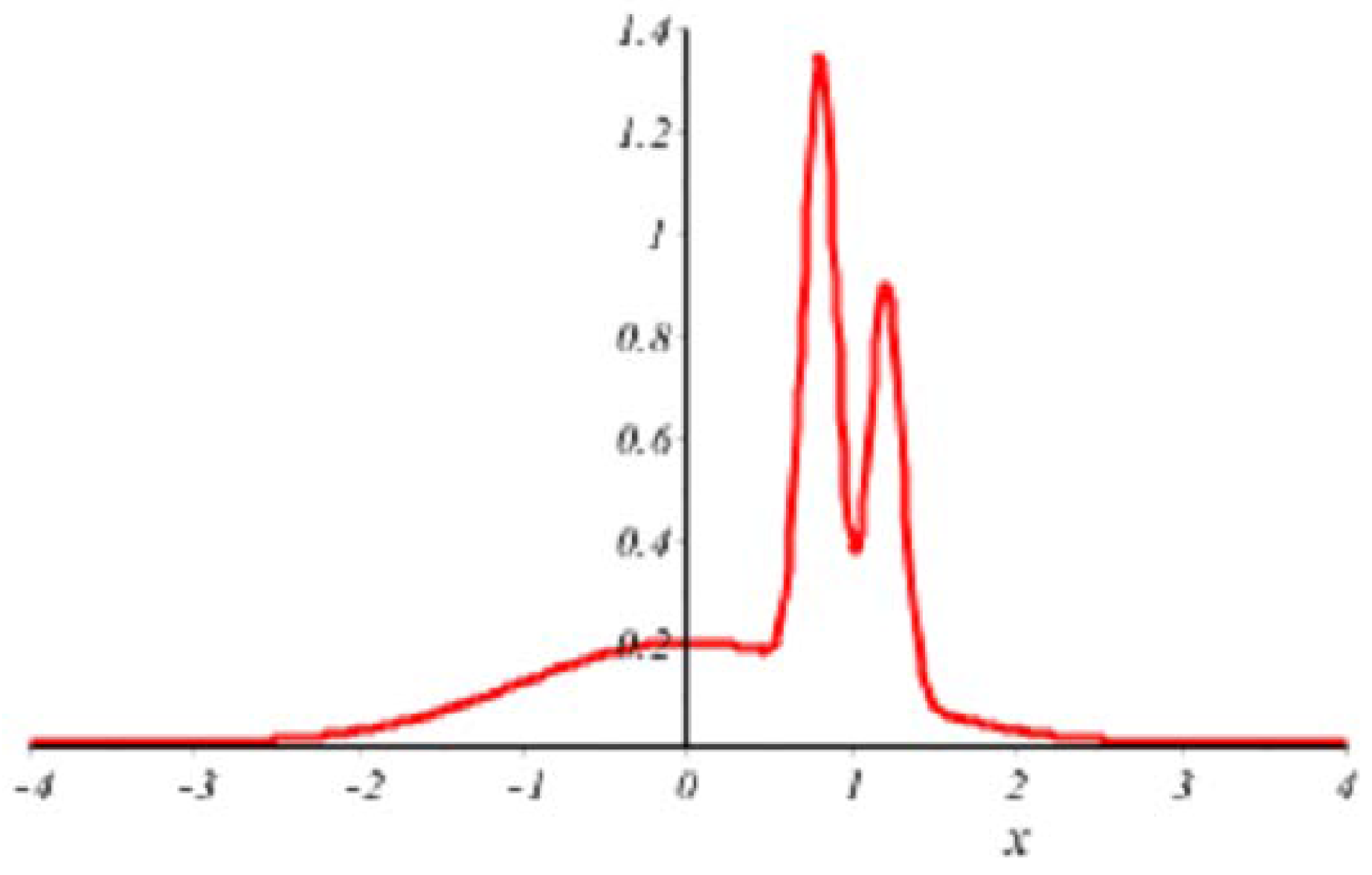
5. An Example
Acknowledgments
Author Contributions
Conflicts of Interest
Appendix A
References
- Silverman, B.W. Density Estimation, for Statistics and Data Analysis; Chapman and Hall: New York, NY, USA, 1986. [Google Scholar]
- Yang, J.; Reeves, A. Bottom-up visual image processing probed with weighted polynomials. Neural Netw. 1995, 8, 669–691. [Google Scholar] [CrossRef]
- Barlow, R.E.; Proschan, F. Mathematical Theory of Reliability; SIAM: Philadelphia, PA, USA, 1996. [Google Scholar]
- Li, Q.; Racine, J.S. Nonparametric Econometrics; Theory and Practice; Princeton University Press: Oxford, UK, 2007. [Google Scholar]
- Koenker, R. Quantile Regression; Cambridge University Press: New York, NY, USA, 2005. [Google Scholar]
- Scott, D.W. Multivariate Density Estimation, Theory, Practice, and Visualization, 2nd ed.; Wiley: New York, NY, USA, 2015. [Google Scholar]
- Hastie, T.; Tibshirani, R.; Friedman, J. The Elememts of Statistical Learning, Dat Mining, Inference, and Prediction; Springer: New York, NY, USA, 2001. [Google Scholar]
- Härdle, W.; Kerkyacharian, G.; Picard, D.; Tsybakov, A. Wavelets, Approximation, and Statistical Applications; Springer: New York, NY, USA, 1998. [Google Scholar]
- Kerman, R.; Huang, M.L.; Brannan, M. Error estimates for Dominici’s Hermite function asymptotic formula and some applications. ANZIAM J. 2009, 50, 550–561. [Google Scholar] [CrossRef]
- Boyd, J.P. Asymptotic coefficients of Hermite function series. J. Comput. Phys. 1984, 54, 382–410. [Google Scholar] [CrossRef]
- Sansone, G. Orthogonal Functions; Pure and Applied Mathematics; Interscience Publishers, Inc.: New York, NY, USA, 1959. [Google Scholar]
- Uspensky, J.V. On the development of arbitrary functions in series of Hermite and Laquerre polynomials. Ann. Math. 1927, 28, 593–619. [Google Scholar] [CrossRef]
- Bedrosian, E. A product theorem for Hilbert transform. Proc. IEEE 1959, 51, 868–869. [Google Scholar] [CrossRef]
- Wiener, N. The Fourier Integral and Certain of Its Applications; Cambridge University Press: New York, NY, USA, 1933. [Google Scholar]

© 2018 by the authors. Licensee MDPI, Basel, Switzerland. This article is an open access article distributed under the terms and conditions of the Creative Commons Attribution (CC BY) license (http://creativecommons.org/licenses/by/4.0/).
Share and Cite
Huang, M.L.; Kerman, R.; Spektor, S. An Estimate of the Root Mean Square Error Incurred When Approximating an f ∈ L2(ℝ) by a Partial Sum of Its Hermite Series. Mathematics 2018, 6, 64. https://doi.org/10.3390/math6040064
Huang ML, Kerman R, Spektor S. An Estimate of the Root Mean Square Error Incurred When Approximating an f ∈ L2(ℝ) by a Partial Sum of Its Hermite Series. Mathematics. 2018; 6(4):64. https://doi.org/10.3390/math6040064
Chicago/Turabian StyleHuang, Mei Ling, Ron Kerman, and Susanna Spektor. 2018. "An Estimate of the Root Mean Square Error Incurred When Approximating an f ∈ L2(ℝ) by a Partial Sum of Its Hermite Series" Mathematics 6, no. 4: 64. https://doi.org/10.3390/math6040064
APA StyleHuang, M. L., Kerman, R., & Spektor, S. (2018). An Estimate of the Root Mean Square Error Incurred When Approximating an f ∈ L2(ℝ) by a Partial Sum of Its Hermite Series. Mathematics, 6(4), 64. https://doi.org/10.3390/math6040064