Forecast Combinations in the Presence of Structural Breaks: Evidence from U.S. Equity Markets

Abstract

Realized volatility, building on the theory of a simple continuous time process, has recently received attention as a nonparametric ex-post estimate of the return variation. This paper addresses the problem of parameter instability due to the presence of structural breaks in realized volatility in the context of three HAR-type models. The analysis is conducted on four major U.S. equity indices. More specifically, a recursive testing methodology is performed to evaluate the null hypothesis of constant parameters, and then, the performance of several forecast combinations based on different weighting schemes is compared in an out-of-sample variance forecasting exercise. The main findings are the following: (i) the hypothesis of constant model parameters is rejected for all markets under consideration; (ii) in all cases, the recursive forecasting approach, which is appropriate in the absence of structural changes, is outperformed by forecast combination schemes; and (iii) weighting schemes that assign more weight in most recent observations are superior in the majority of cases.

1. Introduction

Modeling and forecasting volatility comprise an important issue in empirical finance. Traditional approaches are based on the univariate GARCH class of models or stochastic volatility models. Realized Volatility (RV) has lately become very popular; it uses improved measures of ex-post volatility constructed from high frequency data and provides an efficient estimate of the unobserved volatility of financial markets. In contrast with the GARCH approach, in which the volatility is treated as a latent variable, RV can be considered as an observable proxy, and as a consequence, it can be used in time series models to generate forecasts.

Many authors, staring from [1], have highlighted the importance of structural breaks in RV. Their presence in the data-generating process can induce instability in the model parameters. Ignoring structural breaks and wrongly assuming that the structure of a model remains fixed over time have clear adverse implications. The first finding is the inconsistency of the parameter estimates. Moreover, structural changes are likely to be responsible for most major forecast failures of time-invariant series models. Recently, Kumar [2] has found that volatility transmission from crude oil to equity sectors is structurally unstable and exhibits structural breaks; Gong and Lin [3] have examined whether structural breaks contain incremental information for forecasting the volatility of copper futures, and they have argued that considering structural breaks can improve the performance of most of the existing heterogeneous autoregressive-type models; Ma et al. [4] have introduced Markov regime switching to forecast the realized volatility of the crude oil futures market; in the same context, Wang et al. [5] have found that time-varying parameter models can significantly outperform their constant-coefficient counterparts for longer forecasting horizons.

In this paper, three different model specifications of the log-RV have been considered. The first is the Heterogeneous Autoregressive model (HAR-RV) proposed in [6], which is able to capture many of the features of volatility including long memory, fat tails and self-similarity. The second is the Leverage Heterogeneous Autoregressive model (LHAR-RV) proposed in [7], which is able to approximate both long-range dependence and the leverage effect. The last is the Asymmetric Heterogeneous Autoregressive model (AHAR-RV), which is a simplified version of the model proposed in [1]. In the spirit of the EGARCH model, the AHAR-RV allows for asymmetric effects from positive and negative returns. These models, which have become very popular in the econometric literature on RV, have very parsimonious linear structures, and as a consequence, they are extremely easy to implement and to estimate. Moreover, they have good performance in approximating many features that characterize the dynamics of RV [8], and in the forecasting context, they seem to provide results that are at least as good as more sophisticated models that consider additional components of the realized variance, such as semivariance and jumps [9,10].

The aim of this paper is to empirically investigate the relevance of structural breaks for forecasting RV of a financial time series. The presence of structural breaks in the considered RV-representations has been investigated and verified by resorting to a fluctuation test for parameter instability in a regression context. In particular, attention has been focused on the recursive estimates test [11]. This choice is particularly motivated in those cases where no particular pattern of the deviation from the null hypothesis of constant parameters is assumed. Furthermore, the proposal does not require the specification of the locations of the break points.

In order to handle parameter instability, some specific forecast combinations have been introduced and discussed. They are based on different estimation windows with alternative weighting schemes. These forecast combinations, proposed in a regression setting, are employed in financial time series, highlighting, also in this context, their usefulness in the presence of structural breaks. Moreover, all of them are feasible for a high sample size; they do not explicitly incorporate the estimation of the break dates; and as shown by [12], they do not suffer from this estimation uncertainty.

The forecasting performance of the proposed forecast combinations for the three different specifications of RV models has been compared in terms of two loss functions, the Mean Squared Error (MSE) and the Quasi-Likelihood (QLIKE) described below. These are the loss functions most widely used to compare volatility forecasting performance, and according to [13], they provide robust ranking of the models.

In order to statistically assess if the differences in the forecasting performance of the considered forecast combinations are relevant, the model confidence set, proposed in [14], has been used.

The empirical analysis has been conducted on four U.S. stock market indices: S&P 500, Dow Jones Industrial Average, Russell 2000 and Nasdaq 100. For all the series, the 5-min RV has been considered; it is one of the most used proxies of volatility, and as shown in [15], it favorably compares to more sophisticated alternatives in terms of estimation accuracy of asset price variation.

The structure of this paper is as follows. Section 2 introduces the empirical models for RV and briefly illustrates the problem of structural breaks. In Section 3, some of the most used procedures to test parameters’ instability in the regression framework are reviewed. Attention has been focused on the class of fluctuation tests, and in particular, the recursive estimates test has been discussed. Section 4 introduces the problem of forecasting in the presence of structural breaks and discusses some forecast combinations able to take into account parameters’ instability. In Section 5, the empirical results on the four U.S. stock market indices are reported and discussed. Some final remarks close the paper.

2. Realized Volatility Models

Let $p\left(s\right)$ be the log-price of a financial asset at time s, ${\sigma }^2\left(s\right)$ the instantaneous or spot volatility and $w\left(s\right)$ the standard Brownian motion. Define a simple continuous time process:

$$dp\left(s\right)=\sigma \left(s\right)dw\left(s\right)$$

(1)

and assume that ${\sigma }^2\left(s\right)$ has locally square integrable sample paths, stochastically independent of $w\left(s\right)$. The integrated volatility for day t is defined as the integral of ${\sigma }^2\left(s\right)$ over the interval $(t,t+1)$:

$$I{V}_t={\int }_t^{t+1}{\sigma }^2\left(s\right)ds$$

(2)

where a full twenty four-hour day is represented by Time Interval 1. The integrated volatility is not observable, but it can be estimated using high frequency asset returns.

If m intraday returns are available for each day t, $\left\{r_{t,i}\right\}$$i=1,\dots ,m$, it is possible to define a precise volatility measure, called a realized volatility, as the squared sum of them over day t:

$$R{V}_t=\sum _{i=1}^m{r}_{t,i}^2$$

(3)

If there were no market microstructure noise, the realized volatility would provide a consistent estimator of the integrated volatility, that is as the time interval approaches zero or equivalently m goes to infinity:

$$R{V}_t\to I{V}_t$$

(4)

In this paper, we focus on 5-min realized volatility; this choice is justified on the grounds of past empirical findings that show that at this frequency, there is no evidence of micro-structure noise [16]. Moreover, as shown in [15], 5-min RV favorably compares to more sophisticated alternatives in terms of estimation accuracy.

In the econometric literature, many approaches have been developed to model and forecast realized volatility with the aim of reproducing the main empirical features of financial time series such as long memory, fat tails and self-similarity. In this paper, attention has been focused on the classic Heterogeneous Autoregressive model of Realized Volatility (HAR-RV) and on some of its extensions.

The HAR-RV model, proposed in [6], has a very simple and parsimonious structure; moreover, empirical analysis [8] shows remarkably good forecasting performance. In this model, lags of RV are used at daily, weekly and monthly aggregated periods.

More precisely, let $v_t=log\left(R{V}_t\right)$ where $R{V}_t$ is the realized volatility at time $t=1,2,\dots ,T$. The logarithmic version of the HAR-RV similar to that implemented by [17] is defined as:

$$v_t={\beta }_0+{\beta }_1{v}_{t-1}+{\beta }_2{v}_t^{\left(5\right)}+{\beta }_3{v}_t^{\left(22\right)}+{ϵ}_t$$

(5)

where ${ϵ}_t\sim NID(0,{\sigma }^2)$ and $v_t^{\left(5\right)}$ and $v_t^{\left(22\right)}$ are defined, respectively, as:

$$v_t^{\left(5\right)}=\frac{v_{t-1}+v_{t-2}+\dots +v_{t-5}}{5}$$

(6)

$$v_t^{\left(22\right)}=\frac{v_{t-1}+v_{t-2}+\dots +v_{t-22}}{22}$$

(7)

The HAR-RV model is able to capture some well-known features of financial returns such as long memory and fat tails [8].

The first extension of this model is the Leverage Heterogeneous Autoregressive model of Realized Volatility (LHAR-RV) proposed in [7]. This model is defined as:

$$\begin{array}{cc}{v}_t& ={\beta }_0+{\beta }_1{v}_{t-1}+{\beta }_2{v}_t^{\left(5\right)}+{\beta }_3{v}_t^{\left(22\right)}+{\beta }_4{r}_{t-1}^{-}+{\beta }_5{r}_t^{\left(5\right)-}+\\ & +{\beta }_6{r}_t^{\left(22\right)-}+{\beta }_7{r}_{t-1}^{+}+{\beta }_8{r}_t^{\left(5\right)+}+{\beta }_9{r}_t^{\left(22\right)+}+{ϵ}_t\end{array}$$

(8)

where ${ϵ}_t\sim NID(0,{\sigma }^2)$, $r_t$ are the daily returns and:

$$r_t^{\left(5\right)-}=\frac{r_{t-1}+r_{t-2}+\dots +r_{t-5}}{5}{I}_{\left\{(r_{t-1}+r_{t-2}+\dots +r_{t-5})<0\right\}}$$

(9)

$$r_t^{\left(5\right)+}=\frac{r_{t-1}+r_{t-2}+\dots +r_{t-5}}{5}{I}_{\left\{(r_{t-1}+r_{t-2}+\dots +r_{t-5})>0\right\}}$$

(10)

$$r_t^{\left(22\right)-}=\frac{r_{t-1}+r_{t-2}+\dots +r_{t-22}}{22}{I}_{\left\{(r_{t-1}+r_{t-2}+\dots +r_{t-22})<0\right\}}$$

(11)

$$r_t^{\left(22\right)+}=\frac{r_{t-1}+r_{t-2}+\dots +r_{t-22}}{22}{I}_{\left\{(r_{t-1}+r_{t-2}+\dots +r_{t-22})>0\right\}}$$

(12)

where I is the indicator function. The LHAR-RV model approximates both long-range dependence and the leverage effect. Some authors ([18]) suggest including only the negative part of heterogeneous returns since the estimates of the coefficients of the positive ones are usually not significant.

The second extension is the Asymmetric Heterogeneous Autoregressive model of Realized Volatility (AHAR-RV), which is a simplified version of the model proposed in [1]. It is defined as:

$$v_t={\beta }_0+{\beta }_1{v}_{t-1}+{\beta }_2{v}_t^{\left(5\right)}+{\beta }_3{v}_t^{\left(22\right)}+{\beta }_4\frac{|r_{t-1}|}{\sqrt{R{V}_{t-1}}}+{\beta }_5\frac{|r_{t-1}|}{\sqrt{R{V}_{t-1}}}{I}_{\left\{r_{t-1}<0\right\}}+{ϵ}_t$$

(13)

The last two terms allow for asymmetric effects from positive and negative returns in the spirit of the EGARCH model.

All the considered models can be rewritten in a standard regression framework:

$$y_t={\mathbf{x}}_t^{\prime }\mathit{\beta }+{ϵ}_t$$

(14)

where $y_t=v_t$, ${\mathbf{x}}_t$ is the $p\times 1$ vector of the regressors at time t and $\mathit{\beta }$ is the $p\times 1$ vector of the corresponding coefficients. Of course, the number p and the specification of the vector ${\mathbf{x}}_t$ are different for each model.

Many studies (see, for example, [1]) agree on the existence of structural breaks in RV. If structural breaks are present in the data-generating process, they could induce instability in the model parameters. Ignoring them in the specification of the model could provide the wrong modeling and forecasting for the RV.

To deal with structural breaks, the linear regression model (14) is assumed to have time-varying coefficients, and so, it may be expressed as:

$$y_t={\mathbf{x}}_t^{\prime }{\mathit{\beta }}_t+{ϵ}_{t}t=1,2,\dots T$$

(15)

In many applications, it is reasonable to assume that there are m breakpoints at the date ${\tau }_1,{\tau }_2,\cdots ,{\tau }_m$ in which the coefficients shift from one stable regression relationship to a different one. Thus, there are $m+1$ segments in which the regression coefficients are constant. Model (15) can be rewritten as:

$$y_t={\mathbf{x}}_t^{\prime }{\mathit{\beta }}_{{\tau }_{j-1}+1:{\tau }_j}+{ϵ}_{t}t=1,2,\dots Tj=1,2,\dots m+1$$

(16)

and, by convention, ${\tau }_0=1$ and ${\tau }_{m+1}=T$.

3. Testing for Structural Changes

The presence of structural breaks can be tested through the null hypothesis that the regression coefficients remain constant over time, that is:

$$H_0:{\mathit{\beta }}_t=\mathit{\beta }t=1,2,\dots T$$

(17)

against the alternative that at least one coefficient varies over time.

In the statistical and econometric literature, testing for parameters’ instability in a regression framework has been treated using different approaches. The classical test for structural change is the well-known Chow test [19]. This testing procedure splits the sample into two sub-samples, estimates the parameters for each sub-sample, and then, using a classic F statistic, a test on the equality of the two sets of parameters is performed. For a review, which includes also some extensions in different contexts, see [20]. The principal issue of the Chow test is the assumption that the break-date must be known a priori. Generally, this procedure is used by fixing an arbitrary candidate break-date or by selecting it on the basis of some known feature of the data. However, the results can be highly sensitive to these arbitrary choices; in the first case, the Chow test may be uninformative, and in the second case, it can be misleading [21].

More recently, the literature has focused on a more realistic problem in which the number of break points and their locations are supposed to be unknown (see [22], for a survey). In this context, one of the major contributions is the strategy proposed in Bai and Perron ([23,24,25]) who developed an iterative procedure that allows consistent estimation of the number and the location of the break points together with the unknown regression coefficients in each regime. In their procedure, the breaks are considered deterministic parameters, and so, the specification of their underlying generating process is not required. The number of breaks can be sequentially determined by testing for $q+1$ against q or using a global approach of testing for q against no breaks. However, the procedure needs the specification of some restrictions such as the minimum distance between breaks and their maximum number.

Another approach to change point testing is based on the generalized fluctuation tests (for a survey, see [26]). Such an approach has the advantage of not assuming a particular pattern of deviation from the null hypothesis. Moreover, although it is possible in principal to carry out the location of the break points, this method is commonly used only to verify their presence; with this aim, the fluctuation tests will be used in this paper. The general idea is to fit a regression model to the data and derive the empirical process that captures the fluctuation in the residuals or in the parameter estimates. Under the null hypothesis of constant regression coefficients, fluctuations are governed by functional central limit theorems ([27]), and therefore, boundaries can be found that are crossed by the corresponding limiting processes with fixed probability $\alpha$. When the fluctuation of the empirical process increases, there is evidence of structural changes in the parameters. Moreover, its trajectory may also highlight the type of deviation from the null hypothesis, as well as the dating of the structural breaks. As previously pointed out, the generalized fluctuation tests can be based on the residuals or on the parameter estimates of the regression model. The first class includes the classical CUSUM based on Cumulative Sums of recursive residuals [28], the CUSUM test based on OLS residuals [29] and the Moving Sums (MOSUM) tests based on the recursive and OLS residuals [30]. The second class includes the Recursive Estimates (RE) test [11] and the Moving Estimates (ME) test [31]. In both, the vector of unknown parameters is estimated recursively with a growing number of observations, in the RE test, or with a moving data window, in the ME test, and then compared to the estimates obtained by using the whole sample.

Define:

$${\mathbf{y}}_{1:t}^{\prime }=(y_1,y_2,\dots ,y_t)$$

(18)

$${\mathbf{X}}_{1:t}^{\prime }={({\mathbf{x}}_1,{\mathbf{x}}_2,\dots ,{\mathbf{x}}_t)}^{\prime }$$

(19)

and let:

$${\widehat{\mathit{\beta }}}_{1:t}={\left({\mathbf{X}}_{1:t}^{\prime }{\mathbf{X}}_{1:t}\right)}^{-1}{\mathbf{X}}_{1:t}^{\prime }{\mathbf{y}}_{1:t}t=p,p+1,\dots ,T$$

(20)

be the Ordinary Least Squares (OLS) estimate of the regression coefficients based on the observations up to t.

The basic idea is to reject the null hypothesis of parameter constancy if these estimates fluctuate too much. Formally, the test statistic is defined as:

$$S^{\left(T\right)}=\underset{0\le z\le 1}{sup}{∥B^{\left(T\right)}\left(z\right)∥}_{\infty }$$

(21)

with:

$$B^{\left(T\right)}\left(z\right)=\frac{\varphi \left(z\right)}{\widehat{\sigma }T}{\left({\mathbf{X}}_{1:T}^{\prime }{\mathbf{X}}_{1:T}\right)}^{1/2}({\widehat{\beta }}_{1:\varphi \left(z\right)}-{\widehat{\beta }}_{1:T})$$

(22)

where:

$$\widehat{\sigma }={\left[\frac{1}{T-p}\sum _{t=1}^T(y_t-{\mathbf{x}}_t^{\prime }{\widehat{\beta }}_{1:T})\right]}^{1/2}$$

(23)

and $\varphi \left(z\right)$ is the largest integer less than or equal to $p+z(T-p)$ and ${∥.∥}_{\infty }$ the maximum norm. As proven in [11], $B^{\left(T\right)}\left(z\right)$ is a p-dimensional stochastic process such that

$$B^{\left(T\right)}\left(z\right)\stackrel{\mathcal{D}}{\to }B\left(z\right)$$

(24)

where $B\left(z\right)$ is a Brownian bridge. The distribution of ${sup}_{0\le z\le 1}{∥B\left(z\right)∥}_{\infty }$ is given in [32]; in particular, it is:

$$P\left(\underset{0\le z\le 1}{sup}{∥B\left(z\right)∥}_{\infty }\le x\right)={\left[1+2\sum _{i=1}^{\infty }{(-1)}^i{e}^{-2i^2{x}^2}\right]}^{p}x\ge 0$$

(25)

4. Forecasting Methods in the Presence of Structural Breaks

Once the parameter instability due to the presence of structural breaks has been detected, the problem is how to account for it when generating forecasts. Indeed, parameter instability could cause forecast failures in macroeconomic and financial time series (for a survey, see [33]).

When it is possible to identify the exact date of the last break, the standard solution is to use only observations over the post-break period. In practice, the dates of the break points are not known a priori, and an estimation procedure has to be used. It could produce imprecise values, which negatively affect the specification of the forecasting model and, as a consequence, poor performance of the forecasts. Furthermore, even if the last break date is correctly estimated, the forecasts generated by this scheme are likely to be unbiased and may not minimize the mean square forecast error [12]. Moreover, if the last break is detected close to the boundaries of the data sample, the parameters of the forecasting model are estimated with a relatively short sample, and the estimation uncertainty may be large.

However, as pointed out in [12], the pre-break observations could be informative for forecasting even after the break. More specifically, it is appropriate to choose a high fraction of the pre-break observations especially when the break size is small, the variance parameter increases at the break point and the number of post break observations is small. Furthermore, the forecasting performance is sensitive to the choice of the observation window. A relatively long estimation window reduces the forecast error variance, but increases its bias; on the other hand, a short estimation window produces an increase in the forecast error variance although the bias decreases. Therefore, an optimal window size should balance the trade-off between an accurate estimate of the parameters and the possibility that the data come from different regimes. In this context, Pesaran and Timmermann [12] have proposed some methods to select the window size in the case of multiple discrete breaks when the errors of the model are serially uncorrelated and the regressors are strictly exogenous; Pesaran et al. [34] have derived optimal weights under continuous and discrete breaks in the case of independent errors and exogenous regressors; Giraitis et al. [35] have proposed to select a tuning parameter to downweight older data by using a cross-validation based method in the case of models without regressors; Inoue et al. [36] have suggested to choose the optimal window size that minimizes the conditional Mean Square Forecast Error (MSFE). However, in practice, the selection of a single best estimation window is not an easy task, and in many empirical studies, it is arbitrarily determined.

Alternatively, in order to deal with the uncertainty over the size of the estimation window, it is possible to combine forecasts generated from the same model, but over different estimation windows. This strategy is in the spirit of forecast combinations obtained by estimating a number of alternative models over the same sample period (for a review, see [37]). It has the advantage of avoiding the direct estimation of breakpoint parameters, and it is applicable to general dynamic models and for different estimation methods. In this context, Pesaran and Timmermann [12] have proposed forecast combinations formed by averaging across forecasts generated by using all possible window sizes subject to a minimum length requirement. Based on the same idea, more complex forecasting schemes have been proposed (see, for example, [34,38]).

The idea of forecast averaging over estimation windows has been fruitfully applied also in macroeconomic forecasting, in particular in the context of vector autoregressive models with weakly-exogenous regressors ([39,40] and in the context of GDP growth on the yield curve ([41]).

Pesaran and Pick [42] have discussed the theoretical advantages of using such combinations considering random walks with breaks in the drift and volatility and a linear regression model with a break in the slope parameter. They have shown that averaging forecasts over different estimation windows leads to a lower bias and root mean square forecast error than forecasts based on a single estimation window for all but the smallest breaks. Similar results are reported in [43]; they have highlighted that, in the presence of structural breaks, averaging forecasts obtained by using all the observations in the sample and forecasts obtained by using a window can be useful for forecasting. In this case, forecasts from only two different windows have been combined, and so, this procedure can be seen as a limited version of that proposed in [12].

In view of the above considerations, in this paper, attention has been focused on forecast schemes generated from the same model, but over different estimation windows. In particular, for each of the considered realized volatility models, different forecast combinations have been considered focusing on those that are feasible for financial time series and that do not explicitly incorporate the estimation of the break dates. Moreover, in the analysis, one-step ahead forecasts have been considered, and so, it is assumed that no structural breaks occur in the forecast period (for forecasting with structural breaks over the forecast period, see [44,45]).

4.1. Forecast Combination With Equal Weights

As previously pointed out, the forecast combination with equal weights is the simplest combination, but it is robust to structural breaks of unknown break dates and sizes. Moreover, it performs quite well especially when the break is of moderate magnitude and it is located close to the boundaries of the data sample [42].

Let $\omega$ be the minimum acceptable estimation window size. The forecast combination with equal weights is defined by:

$${\widehat{y}}_{T+1}=\frac{1}{T-\omega }\sum _{\tau =1}^{T-\omega }\left({\mathbf{x}}_{T+1}^{\prime }{\widehat{\mathit{\beta }}}_{\tau +1:T}\right)$$

(26)

Many research works have highlighted the advantages of this scheme; it has good performance also when there is uncertainty about the presence of structural breaks in the data. This approach also avoids any estimation procedure for the weights.

4.2. Forecast Combination With Location Weights

By looking at Equation (26), it is evident that the weights in the equally-weighted combination can be converted into weights on the sample observations ${\mathbf{x}}_t$. As discussed in [38], the $\omega$ most recent observations are used in all of the forecasts, whereas the older observations are used less. Furthermore, the influence of each observation is inversely proportional to its distance from the forecasting origin: the most recent data are usually more relevant especially if the regression parameters have significant changes close to the end of the sample.

A way to place heavier weights on the forecasts that are based on more recent data much more than under the equally-weighted forecast combination is to use constant weights proportional to the location of $\tau$ in the sample.

More precisely, this combination, known as the forecast combination with location weights, is defined by:

$${\widehat{y}}_{T+1}=\frac{1}{{\sum }_{\tau =1}^{T-\omega }\tau }\sum _{\tau =1}^{T-\omega }\tau \left({\mathbf{x}}_{T+1}^{\prime }{\widehat{\mathit{\beta }}}_{\tau +1:T}\right)$$

(27)

Also in this case, no estimation of the weights is needed.

4.3. Forecast Combination With MSFE Weights

This approach, proposed in [12], is based on the idea that the weights of the forecasters obtained with different estimation windows should be proportional to the inverse of the associated out-of-sample MSFE values. To this aim, a cross-validation approach is used.

To better understand, let m be the generic start point of the estimation window and assume that $\tilde{\omega }$ is the number of observations used in the cross-validation set, that is the observations used to measure pseudo out-of-sample forecasting performance. The recursive pseudo out-of-sample MSFE value is computed as:

$$MSFE\left(m\right|T,\tilde{\omega })={\tilde{\omega }}^{-1}\sum _{\tau =T-\tilde{\omega }}^{T-1}{\left(y_{\tau +1}-{\mathbf{x}}_{\tau }^{\prime }{\widehat{\mathit{\beta }}}_{m:\tau }\right)}^2$$

(28)

The forecast combination with MSFE weights is then defined as:

$${\widehat{y}}_{T+1}=\frac{{\sum }_{m=1}^{T-\omega -\tilde{\omega }}\left({\mathbf{x}}_T^{\prime }{\widehat{\beta }}_{m:T}\right){\left(MSFE\left(m\right|T,\tilde{\omega })\right)}^{-1}}{{\sum }_{m=1}^{T-\omega -\tilde{\omega }}{\left(MSFE\left(m\right|T,\tilde{\omega })\right)}^{-1}}$$

(29)

Together with the parameter $\omega$, the length of the minimal estimation window, this method also requires the choice of the parameter $\tilde{\omega }$ and the length of the evaluation window. If this parameter is set too large, too much smoothing may result, and as a consequence, in the combination, the forecasting based on older data will be preferred. On the other hand, if $\tilde{\omega }$ is set too short, although a more precise estimation of the MSFE can be obtained, the ranking of the forecasting methods is more affected by noise. Of course, the selection of this parameter depends on the problem at hand and on the length of the series.

4.4. Forecast Combination With ROC Weights

This approach, proposed in [38], is based on by-products of the Reverse Ordered CUSUM (ROC) structural break test considered in [46].

It is a two-stage forecasting strategy. In the first step, a sequence of ROC test statistics, starting from the most recent observations and going backwards in time, is calculated. Each point in the sample is considered as a possible most recent break point.

This test is related to the classical CUSUM test, but in this case, the test sequence is made in reverse chronological order. In particular, the time series observations are placed in reverse order, and the standard CUSUM test is performed on the rearranged dataset.

In the paper [46], the test statistics are used to perform a formal structural break test and to estimate the last breakpoint in the sample.

In the second step, the ROC statistics are used to weight the associated post break forecast, developing a forecast combination. Moreover, the weights do not depend on finding and dating a structural break, but they are constructed in order to give more weights to observations subsequent to a potential structural break.

In the first step of the procedure, for $\tau =T-\omega +1,T-\omega ,\dots ,2,1$, let:

$${\mathbf{y}}_{T:\tau }^{\prime }=(y_T,y_{T-1},\dots ,y_{\tau +1},y_{\tau })$$

(30)

$${\mathbf{X}}_{T:\tau }^{\prime }=({\mathbf{x}}_T,{\mathbf{x}}_{T-1},\dots ,{\mathbf{x}}_{\tau +1},{\mathbf{x}}_{\tau })$$

(31)

be the observation matrices, and let:

$${\widehat{\mathit{\beta }}}_{T:\tau }^{\left(R\right)}={\left({\mathbf{X}}_{T:\tau }^{\prime }{\mathbf{X}}_{T:\tau }\right)}^{-1}{\mathbf{X}}_{T:\tau }^{\prime }{\mathbf{y}}_{T:\tau }$$

(32)

be a sequence of least squares estimates of $\mathit{\beta }$ associated with the reverse-ordered datasets.

The ROC test statistics $s_t$ are defined as:

$$s_{\tau }=\frac{{\sum }_{t=\tau }^{T-\omega }{\xi }_t^2}{{\sum }_{t=1}^{T-\omega }{\xi }_t^2}\mathrm{for}\tau =T-\omega ,T-\omega -1,\dots ,2,1$$

(33)

where ${\xi }_t$ are the standardized one-step-ahead recursive residuals defined as:

$${\xi }_t=\frac{y_t-{\mathbf{x}}_t^{\prime }{\widehat{\mathit{\beta }}}_{T:t+1}^{\left(R\right)}}{{(1+{\mathbf{x}}_t^{\prime }{\left({\mathbf{X}}_{T:t+1}^{\prime }{\mathbf{X}}_{T:t+1}\right)}^{-1}{\mathbf{x}}_t)}^{1/2}}$$

(34)

In the second step of the procedure, all dates $\tau$ are considered as possible choices for the last breakpoint. The combination weight on each $\tau$ is constructed as:

$$c{w}_{\tau }=\frac{\left|s_{\tau }-\left(\frac{T-\omega -\tau +1}{T-\omega }\right)\right|}{{\sum }_{\tau =1}^{T-\omega }\left|s_t-\left(\frac{T-\omega -\tau +1}{T-\omega }\right)\right|}\tau =1,2,\dots ,T-\omega$$

(35)

Since, under the null hypothesis of no structural break in $\tau$, it is:

$$E\left(s_{\tau }\right)=\frac{T-\omega -\tau +1}{T-\omega }$$

(36)

the combination weights vary according to the absolute distances between $s_{\tau }$ and its expected value. As a consequence, $c{w}_{\tau }$ is larger if this distance is large, that is if the evidence of a structural break is stronger. On the contrary, if in $\tau$, there is no evidence of substantial breakpoint, the associated weight is small.

Moreover, the weights do not depend on finding and dating a structural break. However, if the absolute values of the difference between the ROC statistics and their expectation, under the null hypothesis, start to grow (giving evidence of a potential structural break), the weights $c{w}_{\tau }$ increase giving more weights to the observations on data, subsequent to $\tau$.

The one-step-ahead forecast based on ROC statistics is defined as:

$${\widehat{y}}_{T+1}=\sum _{\tau =1}^{T-\omega }\left(c{w}_{\tau }\left({\mathbf{x}}_{T+1}^{\prime }{\widehat{\mathit{\beta }}}_{\tau +1:T}\right)\right)$$

(37)

4.5. Forecast Combination With ROC Location Weights

In order to take into account a prior belief on the probability that a time $\tau$ could be the most recent break point, it is possible, in the definition of ROC weights, to incorporate an additional weight function $l_{\tau }$.

Following [38], the new weights are defined as:

$$c{w}_{\tau }=\frac{\left|s_{\tau }-\left(\frac{T-\omega -\tau +1}{T-\omega }\right)\right|l_{\tau }}{{\sum }_{\tau =1}^{T-\omega }\left|s_t-\left(\frac{T-\omega -\tau +1}{T-\omega }\right)\right|l_{\tau }}\tau =1,2,\dots ,T-\omega$$

(38)

For example, if a single break point seems to be equally likely at each time point, the natural choice is $l_{\tau }=1$ for $\tau =1,2,\dots ,T-\omega$. In this case, the weights depend only on the magnitude of the ROC statistics, and the combination defined in (37) is obtained.

However, in the forecasting context, where the identification of the most recent break is essential, the prior weight $l_{\tau }$ could be chosen as an increasing function of the location of time $\tau$ in the full sample. In the spirit of forecast combination with location weights, the most natural choice is $l_{\tau }=\tau$. Of course, different specifications are also allowed.

5. Empirical Application

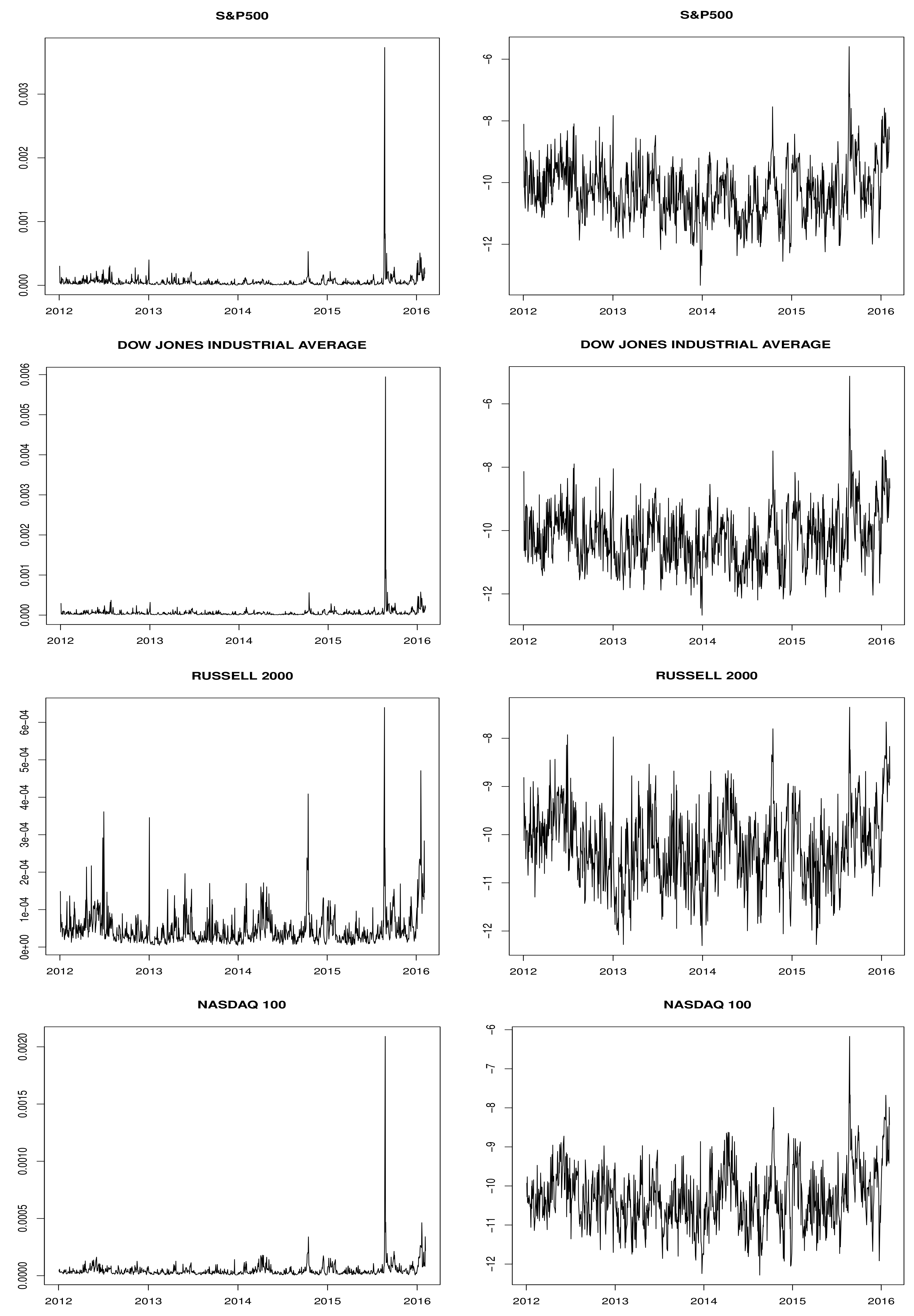
The data were obtained from the Oxford-Man Institute’s Realised library. It consists of 5-min realized volatility and daily returns of four U.S. stock market indices: S&P 500, Dow Jones Industrial Average, Russell 2000 and Nasdaq 100. The sample covers the period from 1 January 2012–4 February 2016; the plots of the RV series and the log-RV series are reported in Figure 1.

In order to investigate the constancy of the regression coefficients in all the considered models (HAR-RV, LHAR-RV and AHAR-RV), an analysis based on the recursive estimates test has been employed for all four series. The results are reported in

Table 1. Recursive estimates test. LHAR, Leverage Heterogeneous Autoregressive model; AHAR, Asymmetric Heterogeneous Autoregressive model; RV, Realized Volatility.

S&P 500			DJIA
Model	statistic	p-value	Model	statistic	p-value
HAR-RV	2.369	0.0001	HAR-RV	2.167	0.0006
LHAR-RV	2.198	0.0010	LHAR-RV	1.943	0.0084
AHAR-RV	2.156	0.0011	AHAR-RV	2.089	0.0019
RUSSELL 2000			NASDAQ 100
Model	statistic	p-value	Model	statistic	p-value
HAR-RV	2.216	0.0004	HAR-RV	1.848	0.0086
LHAR-RV	1.997	0.0048	LHAR-RV	1.659	0.0104
AHAR-RV	2.044	0.0028	AHAR-RV	1.782	0.0093

. The rejection of the null hypothesis of the constancy of the regression parameters for all the models and for all the series is evident.

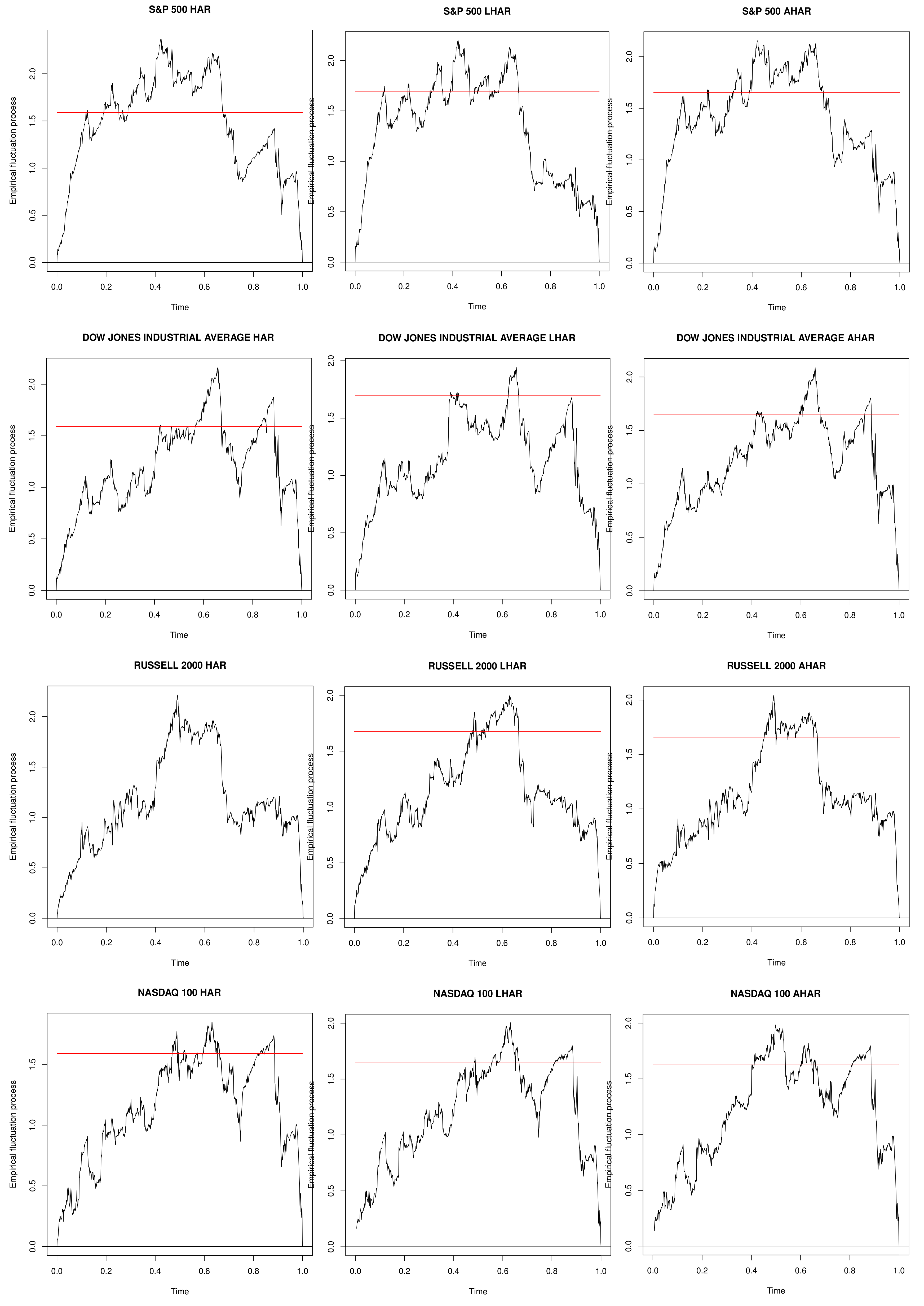
Moreover, in Figure 2, the fluctuation process, defined in Equation (21), is reported for each model specification and for each series, along with the boundaries obtained by its limiting process at level $\alpha =0.05$.

The paths of the empirical fluctuation process confirm the parameters’ instability: the boundaries are crossed for all the series and for all the models.

The above analysis seems to confirm the effectiveness of parameter instability in all three RV-models for all the considered indices. Moreover, it supports the use of forecasting methods that take into account the presence of structural breaks.

In order to evaluate and to compare the forecasting performance of the proposed forecast combinations for each class of model, an initial sub-sample, composed of the data from $t=1$ to $t=R$, is used to estimate the model, and the one-step-ahead out-of-sample forecast is produced. The sample is then increased by one; the model is re-estimated using data from $t=1$ to $t=R+1$; and the one-step-ahead forecast is produced. The procedure continues until the end of the available out-of-sample period. In the following examples, R has been fixed such that the number of out of sample observations is 300. To generate the one-step-ahead forecasts, the five competing forecast combinations, defined in Section 4, have been considered together with a benchmark method.

As a natural benchmark, we refer to the expanding window method, which ignores the presence of structural breaks. In fact, it uses all the available observations. As pointed out in [12], this choice is optimal in situations with no breaks, and it is appropriate for forecasting when the data are generated by a stable model. For each class of models, this method produces out-of-sample forecasts using a recursive expanding estimation window.

Common to all the considered forecast combinations is the specification of the minimum acceptable estimation window size $\omega$. It should not be smaller than the number of regressors plus one; however, as pointed out by [12] , to account for the very large effect of parameter estimation error, it should be at least 3 times the number of unknown parameters. For simplicity, the parameter $\omega$ has been held fixed at 40 for all the RV model specifications.

Moreover, for the MSFE weighted average combination, the length of the evaluation window has been held fixed at 100. This value allows a good estimation of the MSFE and, at the same time, a non-excessive loss of data at the end of the sample where a change point could be very influential for the forecasting.

In order to evaluate the quality of the volatility forecasts, the MSE and the QLIKE loss functions have been considered. They are defined as:

$$\begin{array}{cc}\hfill {\mathrm{MSE}}_t& ={(y_t-{\widehat{y}}_t)}^2\hfill \end{array}$$

(39)

$$\begin{array}{cc}\hfill {\mathrm{QLIKE}}_t& =\frac{y_t}{{\widehat{y}}_t}-log\left(\frac{y_t}{{\widehat{y}}_t}\right)-1\hfill \end{array}$$

(40)

where $y_t$ is the actual value of the 5-min RV at time t and ${\widehat{y}}_t$ is the corresponding RV forecast. They are the most widely-used loss functions, and they provide robust ranking of the models in the context of volatility forecasts [13].

The QLIKE loss is a simple modification of the Gaussian log-likelihood in such a way that the minimum distance of zero is obtained when $y_t={\widehat{y}}_{t+1}$. Moreover, according to [13], it is able to better discriminate among models and is less affected by the most extreme observations in the sample.

These loss functions have been used to rank the six competing forecasting methods for each RV model specification. To this aim, for every method, the average loss and the ratio between its value and the average loss of the benchmark method have been computed. Obviously, a value of the ratio below the unit indicates that the forecasting method “beats” the benchmark according to the loss function metric.

Moreover, to statistically assess if the differences in the performance are relevant, the model confidence set procedure has been used [14].

This procedure is able to construct a set of models from a specified collection, which consists of the best models in terms of a loss function with a given level of confidence, and it does not require the specification of a benchmark. Moreover, it is a stepwise method based on a sequence of significance tests in which the null hypothesis is that the two models under comparison have the same forecasting ability against the alternative that they are not equivalent. The test stops when the first hypothesis is not rejected, and therefore, the procedure does not accumulate Type I error ([14]). The critical values of the test, as well as the estimation of the variance useful to construct the test statistic are determined by using the block bootstrap. This re-sampling technique preserves the dependence structure of the series, and it works reasonably well under very weak conditions on the dependency structure of the data.

In the following, the results obtained for the three different model specifications for the realized volatility of the four considered series are reported and discussed.

Table 2. Out of sample forecasting result for the HAR-RV model. ROC, Reverse Ordered Cumulative Sum.

S&P 500
	MSE	Ratio	rk	MCS	QLIKE	Ratio	rk	MCS
Expanding window	0.5166	1.0000	6	2.154 (0.00)	0.4082	1.0000	6	2.035 (0.00)
MSFE weights	0.5016	0.9710	5	1.010 (1.00)	0.3879	0.9500	4	0.610 (1.00)
ROC weights	0.4986	0.9653	2	−0.956 (1.00)	0.3825	0.9370	2	−0.753 (1.00)
ROC location weights	0.4980	0.9639	1	−1.410 (1.00)	0.3794	0.9294	1	−1.534 (1.00)
Equal weights	0.5015	0.9708	4	0.917 (1.00)	0.3901	0.9557	5	1.191 (0.99)
Location weights	0.5007	0.9694	3	0.437 (1.00)	0.3874	0.9489	3	0.492 (1.00)
DJIA
	MSE	Ratio	rk	MCS	QLIKE	Ratio	rk	MCS
Expanding window	0.6182	1.0000	6	2.112 (0.00)	0.5610	1.0000	6	2.007 (0.00)
MSFE weights	0.6088	0.9849	5	1.344 (0.97)	0.5410	0.9643	4	0.441 (1.00)
ROC weights	0.6066	0.9813	3	−0.213 (1.00)	0.5388	0.9603	2	−0.102 (1.00)
ROC location weights	0.6046	0.9781	1	−1.599 (1.00)	0.5319	0.9480	1	−1.789 (1.00)
Equal weights	0.6079	0.9834	4	0.690 (1.00)	0.5441	0.9699	5	1.208 (1.00)
Location weights	0.6066	0.9813	2	−0.220 (1.00)	0.5402	0.9629	3	0.252 (1.00)
RUSSELL 2000
	MSE	Ratio	rk	MCS	QLIKE	Ratio	rk	MCS
Expanding window	0.3491	1.0000	6	1.904 (0.00)	0.2066	1.0000	6	1.649 (0.00)
MSFE weights	0.3450	0.9881	5	1.235 (0.98)	0.2039	0.9868	4	1.018 (1.00)
ROC weights	0.3445	0.9868	4	0.925 (1.00)	0.2040	0.9872	5	1.071 (0.65)
ROC location weights	0.3424	0.9808	2	−0.548 (1.00)	0.2011	0.9733	2	−0.702 (1.00)
Equal weights	0.3430	0.9826	3	−0.106 (1.00)	0.2025	0.9798	3	0.123 (1.00)
Location weights	0.3410	0.9768	1	−1.500 (1.00)	0.1998	0.9670	1	−1.507 (1.00)
NASDAQ 100
	MSE	Ratio	rk	MCS	QLIKE	Ratio	rk	MCS
Expanding window	0.3509	1.0000	6	2.061 (0.00)	0.2397	1.0000	6	1.897 (0.00)
MSFE weights	0.3448	0.9825	4	1.007 (1.00)	0.2307	0.9697	5	1.106 (1.00)
ROC weights	0.3449	0.9829	5	1.130 (1.00)	0.2319	0.9676	4	0.907 (1.00)
ROC location weights	0.3433	0.9784	3	−0.229 (1.00)	0.2285	0.9535	2	−0.484 (1.00)
Equal weights	0.3432	0.9781	2	−0.319 (1.00)	0.2300	0.9595	3	0.108 (1.00)
Location weights	0.3417	0.9738	1	−1.578 (1.00)	0.2257	0.9417	1	−1.631 (1.00)

Note: For both the loss functions (MSE and QLIKE), the entries are: the values of the average loss; the ratio of the average loss to that of the expanding window method; the rank (rk) according to the average loss function; the statistic and the p-value of the Model Confidence Set (MCS) procedure with $\alpha =0.10$. A bold entry denotes the value of the smallest average loss.

,

Table 3. Out of sample forecasting result for the LHAR-RV model.

S&P 500
	MSE	Ratio	rk	MCS	QLIKE	Ratio	rk	MCS
Expanding window	0.4247	1.0000	5	1.776 (0.00)	0.2858	1.0000	6	2.143 (0.00)
MSFE weights	0.4176	0.9834	1	−1.258 (1.00)	0.2666	0.9328	3	1.316 (0.01)
ROC weights	0.4183	0.9851	2	−0.617 (1.00)	0.2657	0.9298	1	−0.632 (1.00)
ROC location weights	0.4204	0.9899	4	1.275 (0.13)	0.2658	0.9301	2	0.618 (0.55)
Equal weights	0.4197	0.9882	3	0.599 (1.00)	0.2678	0.9370	4	1.557 (0.00)
Location weights	0.4260	1.0031	6	1.536 (0.00)	0.2695	0.9430	5	1.673 (0.00)
DJIA
	MSE	Ratio	rk	MCS	QLIKE	Ratio	rk	MCS
Expanding window	0.5291	1.0000	5	1.191 (0.09)	0.4236	1.0000	6	1.998 (0.00)
MSFE weights	0.5255	0.9932	1	−1.181 (1.00)	0.4012	0.9471	3	1.368 (0.00)
ROC weights	0.5260	0.9942	2	−0.844 (1.00)	0.3996	0.9433	1	−0.913 (1.00)
ROC location weights	0.5290	0.9998	4	1.092 (0.57)	0.3999	0.9440	2	0.912 (0.44)
Equal weights	0.5268	0.9957	3	−0.311 (1.00)	0.4063	0.9592	4	1.633 (0.00)
Location weights	0.5325	1.0063	6	1.783 (0.00)	0.4091	0.9658	5	1.522 (0.00)
RUSSELL 2000
	MSE	Ratio	rk	MCS	QLIKE	Ratio	rk	MCS
Expanding window	0.3096	1.0000	6	2.082 (0.00)	0.1828	1.0000	6	1.564 (0.00)
MSFE weights	0.3058	0.9877	5	1.783 (0.00)	0.1821	0.9964	5	1.464 (0.00)
ROC weights	0.3044	0.9833	4	0.777 (1.00)	0.1809	0.9895	4	1.334 (0.00)
ROC location weights	0.3035	0.9805	1	−1.676 (1.00)	0.1794	0.9812	2	−0.989 (1.00)
Equal weights	0.3044	0.9832	3	0.686 (1.00)	0.1804	0.9867	3	1.268 (0.00)
Location weights	0.3042	0.9827	2	0.210 (1.00)	0.1789	0.9786	1	−0.993 (1.00)
NASDAQ 100
	MSE	Ratio	rk	MCS	QLIKE	Ratio	rk	MCS
Expanding window	0.3180	1.0000	6	2.083 (0.00)	0.2070	1.0000	6	1.984 (0.00)
MSFE weights	0.3112	0.9787	4	1.058 (0.99)	0.1979	0.9562	5	1.066 (1.00)
ROC weights	0.3113	0.9788	5	1.086 (0.99)	0.1977	0.9551	4	0.970 (1.00)
ROC location weights	0.3099	0.9747	3	−0.034 (1.00)	0.1947	0.9406	2	−0.315 (1.00)
Equal weights	0.3093	0.9726	2	−0.586 (1.00)	0.1953	0.9436	3	−0.047 (1.00)
Location weights	0.3082	0.9691	1	−1.516 (1.00)	0.1915	0.9252	1	−1.665 (1.00)

Note: For both loss functions (MSE and QLIKE), the entries are: the values of the average loss; the ratio of the average loss to that of the expanding window method; the rank (rk) according to the average loss function; the statistic and the p-value of the Model Confidence Set procedure with $\alpha =0.10$. A bold entry denotes the value of the smallest average loss.

and

Table 4. Out of sample forecasting result for the AHAR-RV model.

S&P 500
	MSE	Ratio	rk	MCS	QLIKE	Ratio	rk	MCS
Expanding window	0.4576	1.0000	6	2.186 (0.00)	0.3315	1.0000	6	2.151 (0.00)
MSFE weights	0.4397	0.9608	5	1.230 (0.94)	0.3072	0.9267	5	1.268 (0.00)
ROC weights	0.4371	0.9552	2	−0.860 (1.00)	0.3043	0.9179	3	1.393 (0.00)
ROC location weights	0.4364	0.9537	1	−1.416 (1.00)	0.3012	0.9085	1	−0.973 (1.00)
Equal weights	0.4391	0.9596	4	0.781 (1.00)	0.3063	0.9240	4	1.413 (0.00)
Location weights	0.4385	0.9582	3	0.252 (1.00)	0.3016	0.9097	2	−0.977 (0.38)
DJIA
	MSE	Ratio	rk	MCS	QLIKE	Ratio	rk	MCS
Expanding window	0.5669	1.0000	6	2.189 (0.00)	0.4718	1.0000	6	2.091 (0.00)
MSFE weights	0.5534	0.9762	5	1.015 (0.99)	0.4418	0.9365	5	0.986 (1.00)
ROC weights	0.5529	0.9754	3	0.291 (1.00)	0.4404	0.9335	3	0.688 (1.00)
ROC location weights	0.5516	0.9731	1	−1.744 (1.00)	0.4308	0.9132	1	−1.337 (1.00)
Equal weights	0.5532	0.9758	4	0.679 (0.99)	0.4407	0.9341	4	0.749 (1.00)
Location weights	0.5526	0.9748	2	−0.219 (1.00)	0.4320	0.9158	2	−1.083 (1.00)
RUSSELL 2000
	MSE	Ratio	rk	MCS	QLIKE	Ratio	rk	MCS
Expanding window	0.3193	1.0000	6	1.964 (0.00)	0.1898	1.0000	6	1.706 (0.00)
MSFE weights	0.3132	0.9811	5	1.498 (0.00)	0.1868	0.9842	5	1.348 (0.00)
ROC weights	0.3113	0.9750	4	1.183 (0.19)	0.1854	0.9769	4	1.385 (0.00)
ROC location weights	0.3086	0.9665	2	−0.735 (1.00)	0.1824	0.9610	2	0.995 (0.20)
Equal weights	0.3107	0.9731	4	0.760 (1.00)	0.1849	0.9741	3	1.385 (0.00)
Location weights	0.3079	0.9644	1	−1.204 (1.00)	0.1818	0.9579	1	−0.995 (1.00)
NASDAQ 100
	MSE	Ratio	rk	MCS	QLIKE	Ratio	rk	MCS
Expanding window	0.3299	1.0000	6	2.078 (0.00)	0.2223	1.0000	6	1.992 (0.00)
MSFE weights	0.3207	0.9719	4	0.825 (1.00)	0.2122	0.9545	4	0.936 (1.00)
ROC weights	0.3213	0.9738	5	1.212 (1.00)	0.2125	0.9560	5	1.073 (1.00)
ROC location weights	0.3192	0.9675	3	−0.092 (1.00)	0.2088	0.9394	2	−0.429 (1.00)
Equal weights	0.3189	0.9665	2	−0.298 (1.00)	0.2101	0.9451	3	0.085 (1.00)
Location weights	0.3167	0.9599	1	−1.643 (1.00)	0.2058	0.9257	1	−1.651 (1.00)

Note: For both loss functions (MSE and QLIKE), the entries are: the values of the average loss; the ratio of the average loss to that of the expanding window method; the rank (rk) according to the average loss function; the statistic and the p-value of the Model Confidence Set (MCS) procedure with $\alpha =0.10$. A bold entry denotes the value of the smallest average loss.

provide the results of the analysis for the HAR-RV, LHAR-RV and AHAR-RV model specification respectively for the four considered series. In particular, they report the average MSE and the average QLIKE for each forecasting method, as well as their ratio for an individual forecasting method to the benchmark expanding window method and the ranking of the considered methods with respect to each loss function. Moreover, the value of the test statistic of the model confidence set approach and the associated p-value are also reported.

In the case of the HAR model, for all the considered series and for both loss functions, there is significant evidence that all the forecast combinations have better forecasting ability with respect to the expanding window procedure; the ratio values are all less than one. Moreover, for both loss functions, the best method is the forecast combination with ROC location weights for S&P 500 and Dow Jones Industrial Average and with location weights for Russell 2000 and Nasdaq 100; this result confirms the importance of placing heavier weights on the forecast based on more recent data.

The model confidence set has the same structure for all four series and for both loss functions; it excludes only the forecast generated by the expanding window procedure and includes all the forecast combinations.

For the LHAR model, focusing on the results of S&P 500 and Dow Jones Industrial Average, which have very similar behavior, the forecast combination with MSFE weights offers the best improvement in forecasting accuracy according to the MSE metric, while the forecast combination with ROC weights according to the QLIKE metric.

For Russell 2000, the forecast combination with ROC location weights beats all the competing models according to MSE loss function, while, under the QLIKE, the best method is the forecast combination with location weights. This last method has better performance with respect to both of the loss function metrics for Nasdaq 100.

By looking at the MSE ratios for S&P 500 and Dow Jones Industrial Average Index, it is evident that the forecast combination with location weights is unable to beat the expanding window procedure; for all the others, the combinations are able to outperform it consistently.

In the model confidence set, when the MSE loss function is used, the expanding window is eliminated from the model confidence set for all the series. However, the forecast combination with location weights for S&P 500 and Dow Jones Industrial Average and that with MSFE weights for Russell 2000 are also eliminated. A quite different situation arises when the loss function QLIKE is considered. In this case, the only surviving models in the model confidence set are the two combinations based on ROC statistics for S&P 500 and Dow Jones Industrial Average and those based on ROC location weights and on location weights for Russell 2000. For Nasdaq 100, all the combinations have the same forecasting accuracy. Excluding the last case, the QLIKE loss function, as pointed out previously, seems to better discriminate among forecasting methods.

Finally, in the case of the AHAR model, in line with the previous results, the expanding window appears to offer the worst forecasting performance overall.

Moreover, for both MSE and QLIKE loss functions, the method that offers the major improvement in forecasting accuracy is the forecast combination with ROC location weights for S&P 500 and Dow Jones Industrial Average Index and the the forecast combination with location weights for Russell 2000 and Nasdaq 100.

Focusing on the model confidence set, for the MSE loss function, the expanding window is always eliminated for all the series together with the forecast combination with MSFE weights for Russell 2000. With respect to the QLIKE loss function, for Dow Jones Industrial Average Index and Nasdaq 100, the only excluded method is the expanding window procedure. For the other series, the results confirm the better discriminative property of the QLIKE metric; the only surviving methods are forecast combination with ROC location weights and with location weights.

In conclusion, even if it is not clear which combination has the best forecasting performance, the forecast combination with ROC location weights and that with location weights seems to be always among the best methods. However, the forecast combination with ROC location weights always outperforms the expanding window method, and it is always in the top position with respect to the loss function ratio and is never excluded by the model confidence set.

6. Concluding Remarks

This paper has explored the relevance of taking into account the presence of structural breaks in forecasting realized volatility. The analysis has been based on 5-min realized volatility of four U.S. stock market indices: S&P 500, Dow Jones Industrial Average, Russell 2000 and Nasdaq 100. Three different model specifications of the log-realized volatility have been considered. For all the considered market indices, the instability in the parameters of the RV models has been verified through the recursive estimates test. In order to handle this problem, five forecast combinations, based on different estimation windows with alternative weighting schemes, have been introduced and compared with the expanding window method, a natural choice when the data are generated by a stable model. The forecasting performance has been evaluated, for each RV model specification, through two of the most relevant loss functions, the MSE and the QLIKE. Moreover, to this aim, the average loss function has been calculated, and in order to statistically assess if the differences in the performance are relevant, the model confidence set approach has been considered.

The analysis, repeated for each class of RV models separately, has highlighted the importance of taking into account structural breaks; in fact, the expanding window appears to offer the worst forecasting performance overall. In particular, in almost all the considered cases, the two combinations that make adjustments for accounting for the most recent possible break point (the forecast combination with location weights and with ROC location weights) are placed in first position and, as a consequence, have better forecasting performance. Nevertheless, the forecast combination with ROC location weights always outperforms the expanding window method; it is always in the top position with respect to the loss function ratio, and it is never excluded by the model confidence set.