Article

Symmetric Radial Basis Function Method for Simulation of Elliptic Partial Differential Equations

1
Renewable Energy Research Centre & Department of Teacher Training in Electrical Engineering, Faculty of Technical Education, King Mongkut’s University of Technology North Bangkok (KMUTNB), Wongsawang, Bangsue, Bangkok 10800, Thailand
2
Department of Basic Sciences, University of Engineering and Technology, Peshawar 25000, Pakistan
3
KMUTT-Fixed Point Theory and Applications Research Group, Theoretical and Computational Science Center (TaCS), Science Laboratory Building, Faculty of Science, King Mongkut’s University of Technology Thonburi (KMUTT), 126 Pracha-Uthit Road, Bang Mod, Thrung Khru, Bangkok 10140, Thailand
*
Author to whom correspondence should be addressed.
Mathematics 2018, 6(12), 327; https://doi.org/10.3390/math6120327
Submission received: 8 October 2018 / Revised: 28 November 2018 / Accepted: 8 December 2018 / Published: 14 December 2018
(This article belongs to the Special Issue Numerical Methods for Partial Differential Equations)

Abstract

:
In this paper, the symmetric radial basis function method is utilized for the numerical solution of two- and three-dimensional elliptic PDEs. Numerical results are obtained by using a set of uniform or random points. Numerical tests are accomplished to demonstrate the efficacy and accuracy of the method on both regular and irregular domains. Furthermore, the proposed method is tested for the solution of elliptic PDE in the case of various frequencies.

1. Introduction

A considerable number of science and engineering problems with suitable boundary conditions are managed by elliptic partial differential equations (EPDEs). EPDEs arise in many time-independent physical problems such as steady-state problems involving incompressible fluids, the steady-state distribution of heat in a plane region, while microwaves, as well as acoustic waves could be simulated by the Helmholtz equation. Generally, it is hard to attain the closed-form solutions of such equations.
Owing to this fact, several proficient and precise methods have been developed for the numerical solution of EPDEs. Contemporary contributions in this regard comprise spline collocation methods [1,2], the finite element method [3], finite difference methods [4,5], the wavelet collocation method [6], meshless methods [7,8,9], etc.
A broad variety of meshless methods underway is based on radial basis functions (RBF) [9,10,11,12]. The simplest among them is unsymmetric RBF collocation or the Kansa method [13]. When the goal is to approximate dispersed data in several dimensions, the RBF methods in the case of multivariate approximation turn out to be the most frequently-applied methodology. The global, non-polynomial, RBF method is a valuable substitute for obtaining exponential accuracy where classical methods are hard to apply or fail. In multifaceted problems, non-rectangular domains comprise an instance. To compose a univariate function with the Euclidean norm, the RBF methods turns out to perform well in extremely common settings. Consequently, a multidimensional problem can be effectively altered into one-dimensional.
A vast range of problems has been successfully solved by the Kansa method. However, there is no prescribed guarantee for the standard formulation that the collocation unsymmetric matrix will be non-singular [14]. In particular, to get a non-singular collocation matrix, a small perturbation of functional center locations is also useful [15]; whereas, numerical ill-conditioning issues may be possible in the perturbed collocation matrix.
Fasshauer [16] proposed an alternate method, the PDE operator, which has been applied to the RBF as the basis function, known as the Hermitian or symmetric RBF (SRBF) method, which yields a symmetric collocation matrix (thus attractive for the benefits of storage) and was shown by Wu [17] to be nonsingular only if no two collocation points sharing the same operator were placed in the same location.
The SRBF method has several advantages over the Kansa method, but Robert Shaback [18] has shown that both methods experience the same basic problem, the uncertainty relation; good conditioning is related to inferior accuracy, and inferior conditioning is related to better accuracy. In the case of increasing the system size, this problem turns out to be more distinct. To avoid this problem, much of the research has been dedicated in recent years to the formulation of RBF-specific pre conditioners [15], the adaptive selection of functional centers, and collocation points [14].
The SRBF method has a benefit over the Kansa method that the collocation matrices are symmetric. Therefore, the computation cost can be significantly decreased, which is vital for larger problems. Different problems have been solved using the SRBF method [19,20,21,22].

2. Governing Equations

We consider the following governing equations.
The Poisson equation:
L u ( x ) = Δ u ( x ) = f ( x ) , x Ω n ,
with boundary conditions:
B 1 ( x ) = f 1 ( x ) , x Ω ,
where L = Δ .
The Helmholtz equation:
L u ( x ) = Δ u ( x ) + k u ( x ) = g ( x ) , x Ω n ,
with boundary conditions:
B 2 ( x ) = g 1 ( x ) , x Ω ,
where L = Δ + k .
Δ is the Laplace operator, and n is the dimension of the spatial variable in both cases.

3. Numerical Scheme

In the SRBF method, an approximate solution is sought of the form [16]:
u ( x ) = λ 1 ϕ ( | x x 1 | ) + i = 2 N 1 λ i L 2 ϕ ( | x x i | ) + λ N ϕ ( | x x N | ) ,
where L 2 is a linear differential operator similar to L , but acting on ϕ as a function of the second variable x i . Using Equation (5) on the one-dimensional elliptic PDE with boundary conditions given by:
L u ( x ) = f ( x ) , a < x < b , u ( a ) = u a , u ( b ) = u b ,
enforcing the collocation conditions at the interior points, i = 2 , 3 , , N 1 , we get the system of linear equations:
λ 1 ϕ ( | a x 1 | ) + i = 2 N 1 λ i L 2 ϕ ( | a x i | ) + λ N ϕ ( | a x N | ) = u a , λ 1 L ϕ ( | x x 1 | ) + i = 2 N 1 λ i L L 2 ϕ ( | x x i | ) + λ N L ϕ ( | x x N | ) = f ( x ) , x [ a , b ] , λ 1 ϕ ( | b x 1 | ) + i = 2 N 1 λ i L 2 ϕ ( | b x i | ) + λ N ϕ ( | b x N | ) = u b .
In matrix notation, we can write:
A λ = B ,
where:
A = A L L 2 A L A L 2 A , λ = [ λ 1 , λ 2 , , λ N ] T , B = [ u a , f ( x 2 ) , f ( x 3 ) , , f ( x N 1 ) , u b ] T .
Here, the four blocks in matrix A are generated as follows:
( A L L 2 ) i j = L L 2 ϕ ( x i x j ) , x i , x j Ω 1 , ( A L ) i j = L ϕ ( x i x j ) , x i Ω 1 , x j Ω 2 , ( A L 2 ) i j = L 2 ϕ ( x i x j ) , x i Ω 2 , x j Ω 1 , A i j = ϕ ( x i x j ) , x i , x j Ω 2 ,
where Ω 1 and Ω 2 are interior and boundary nodes, respectively.

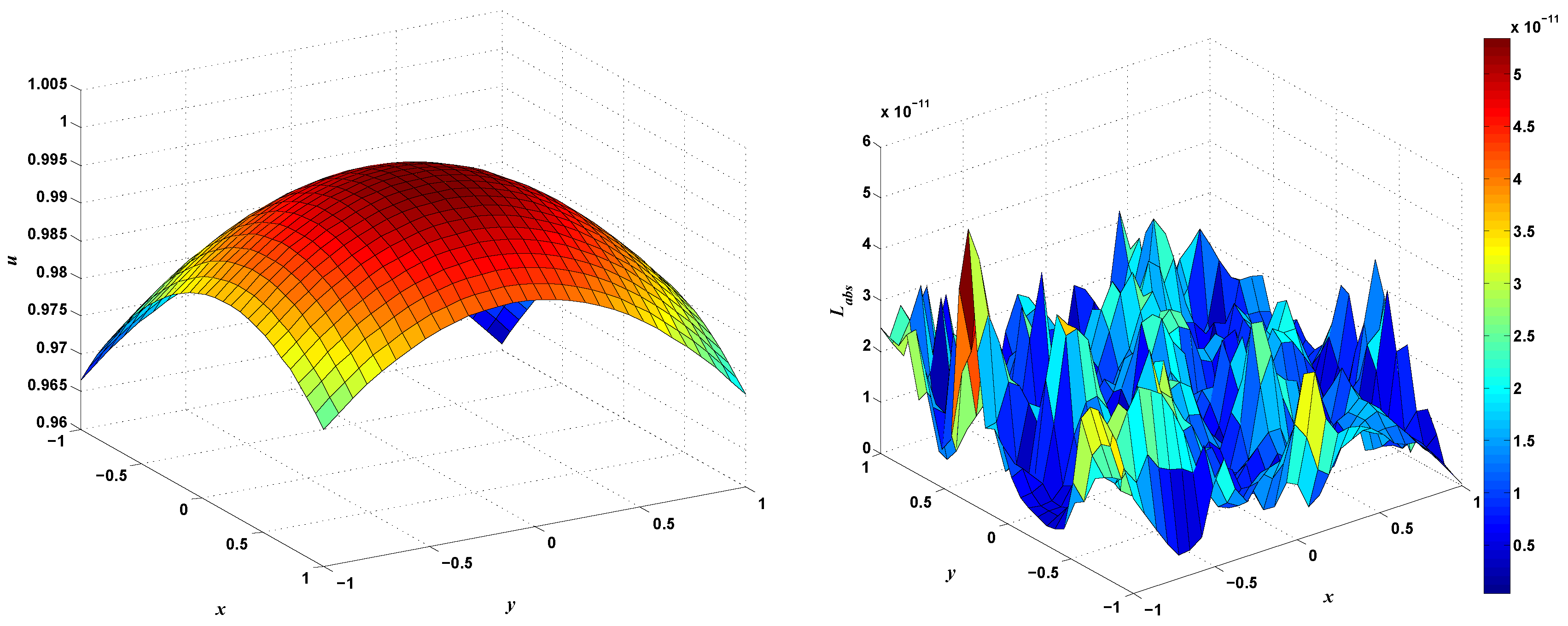
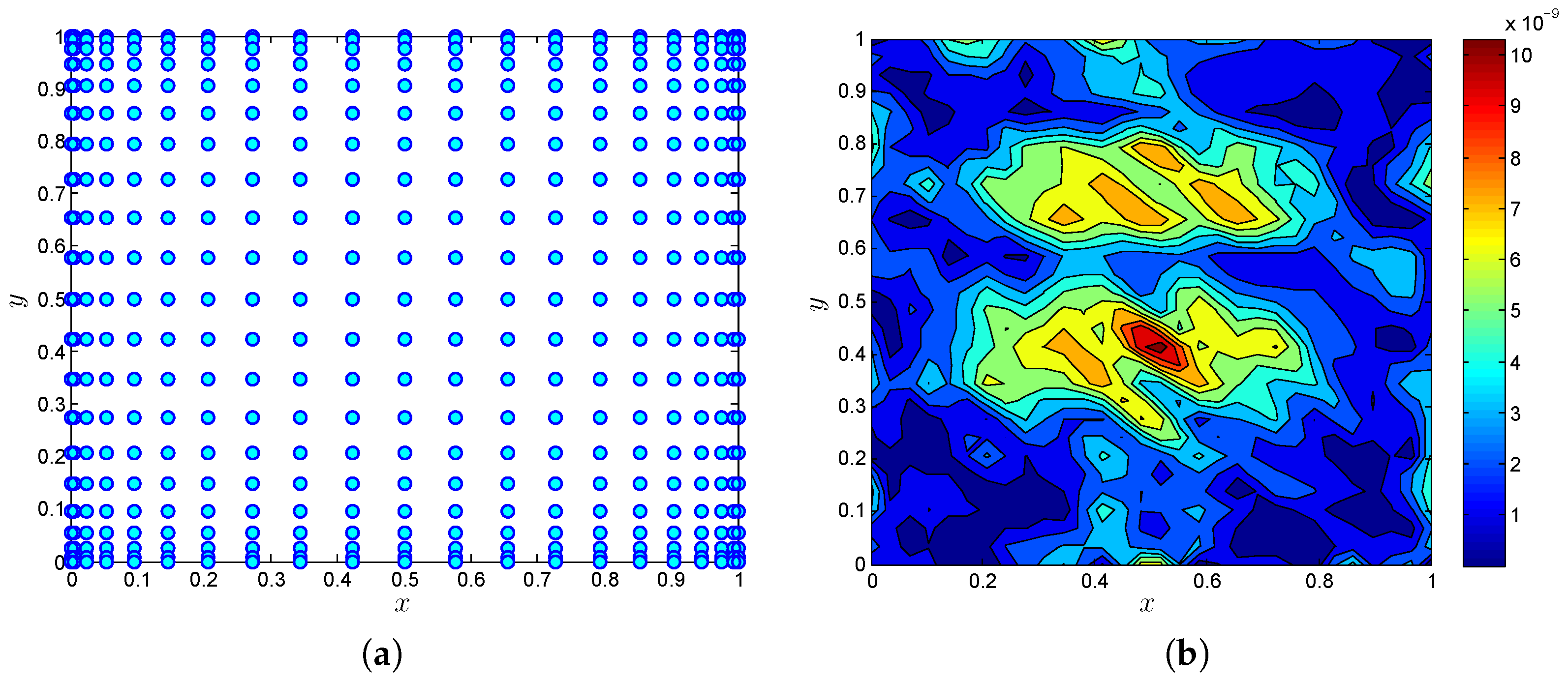
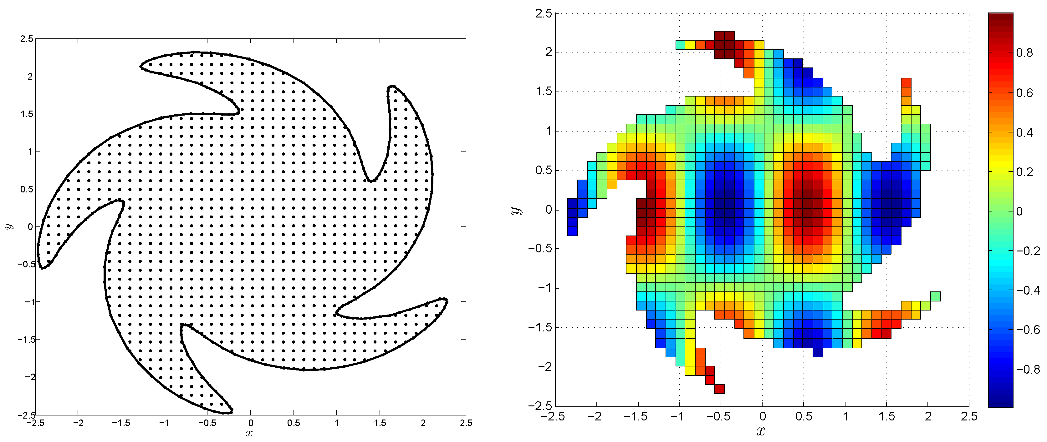
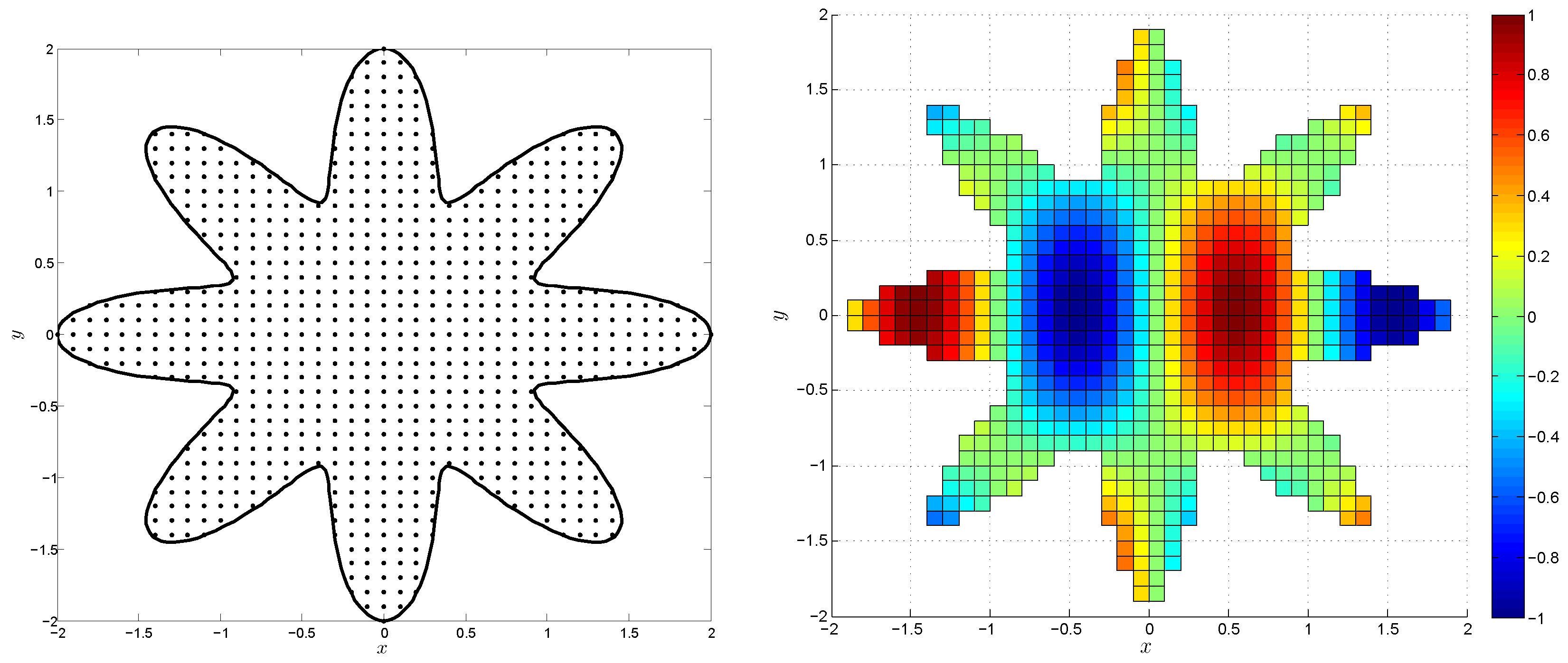
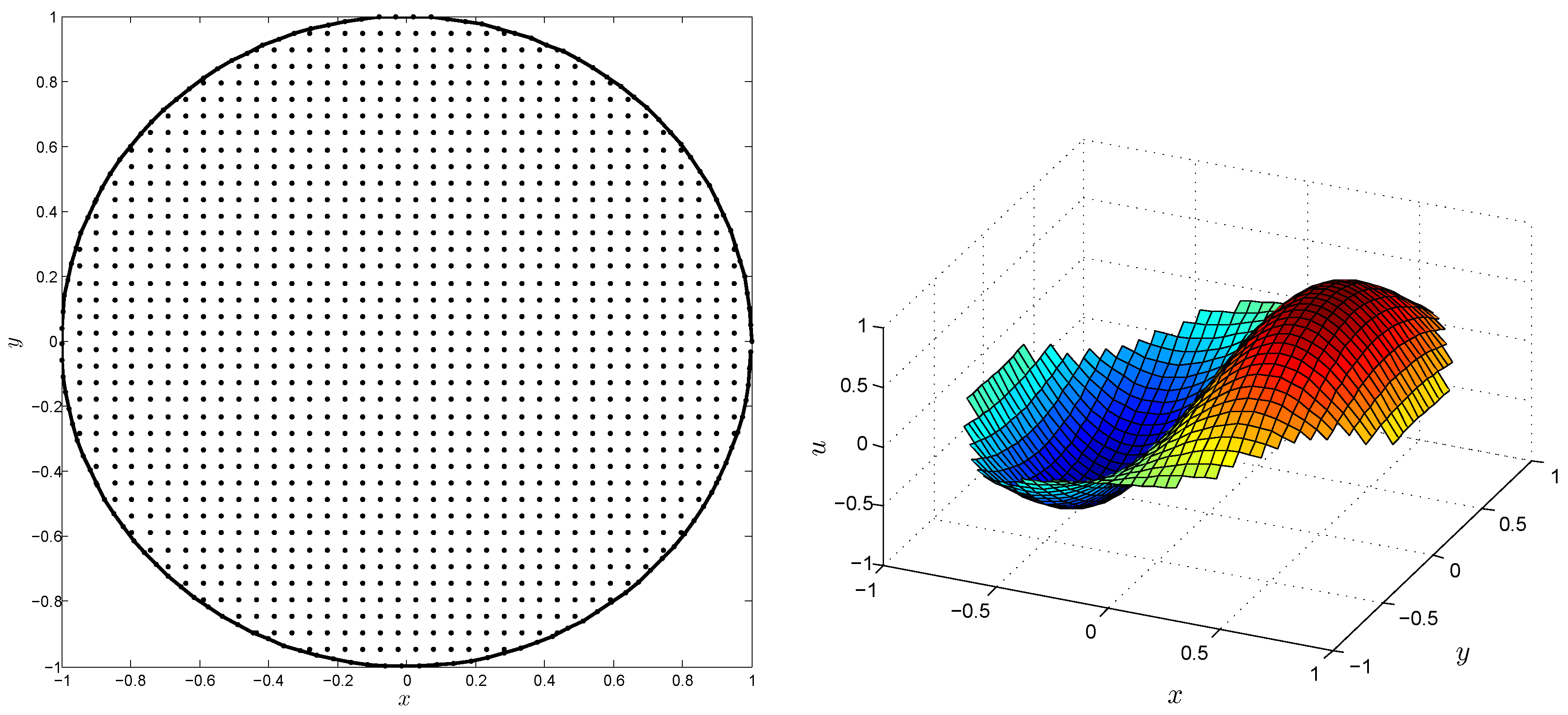
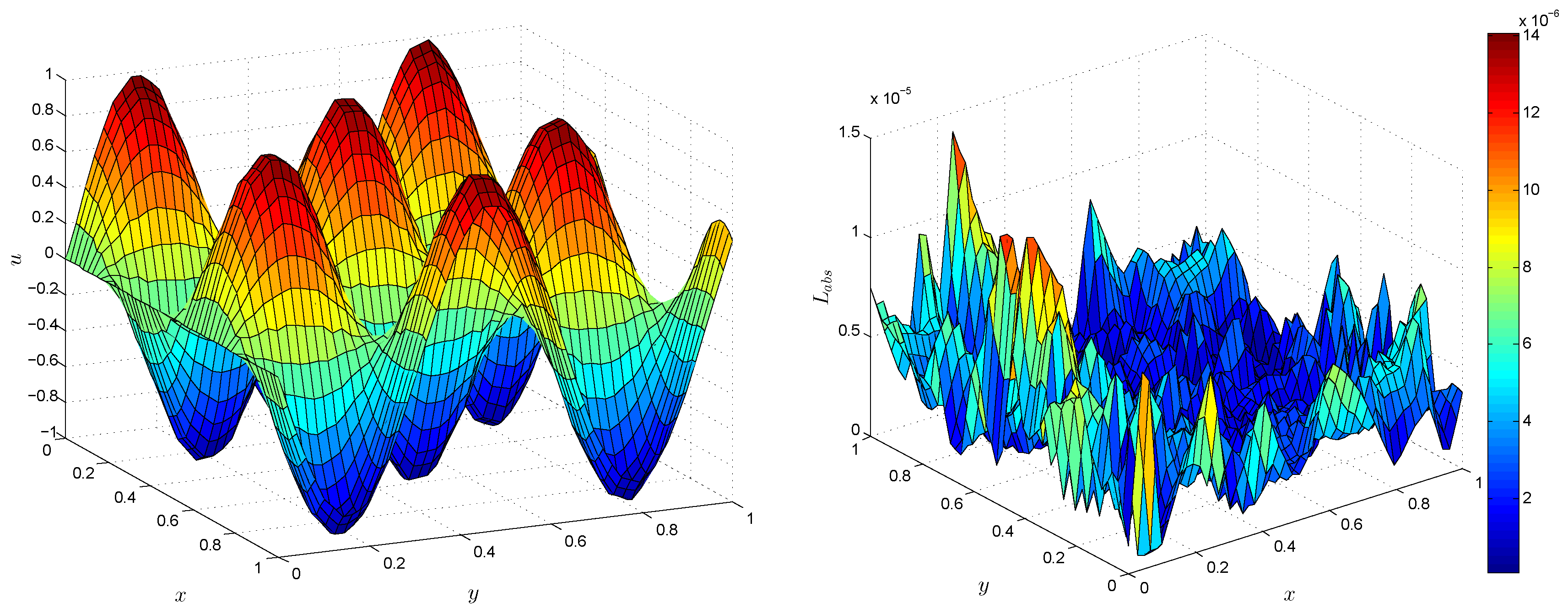
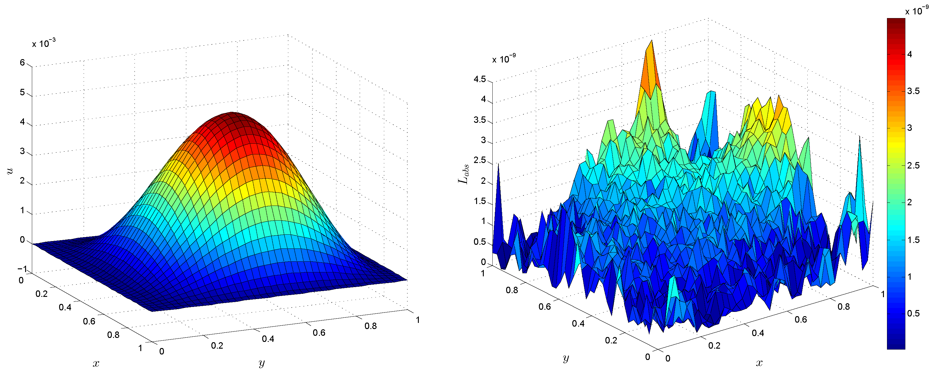
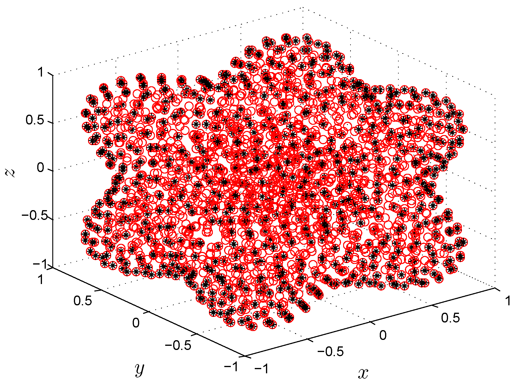
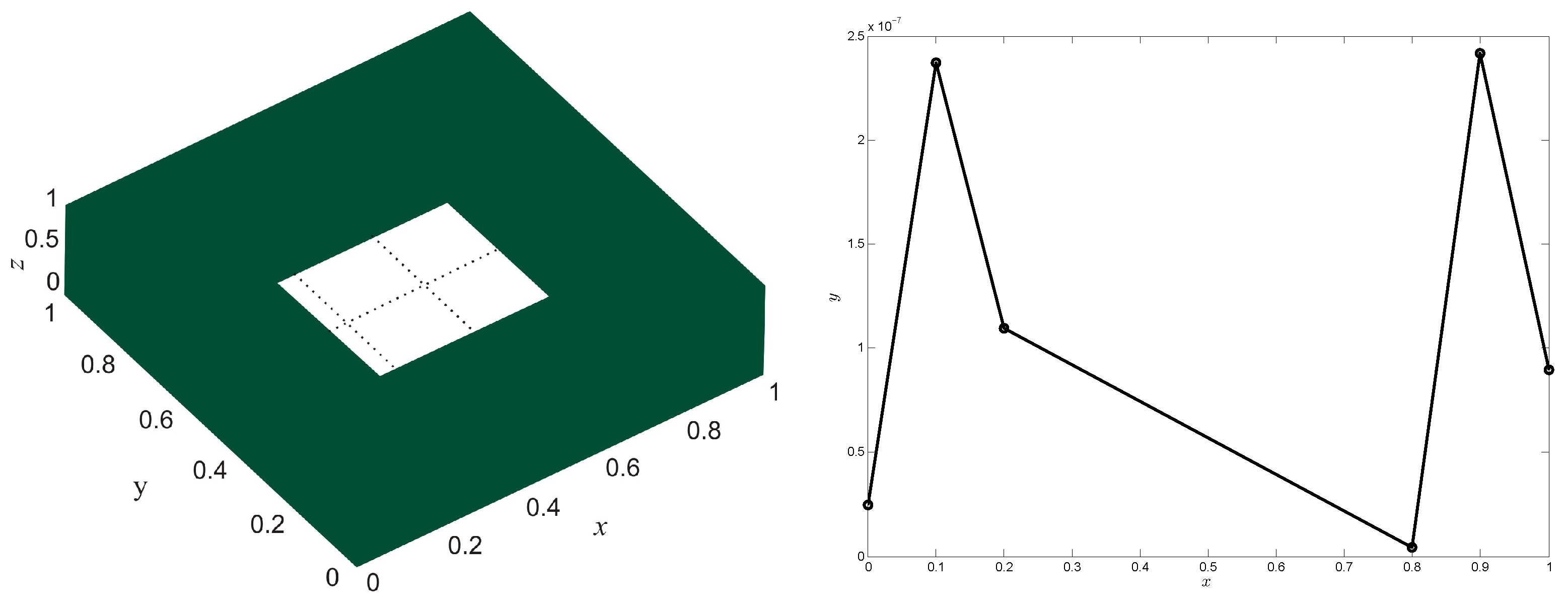
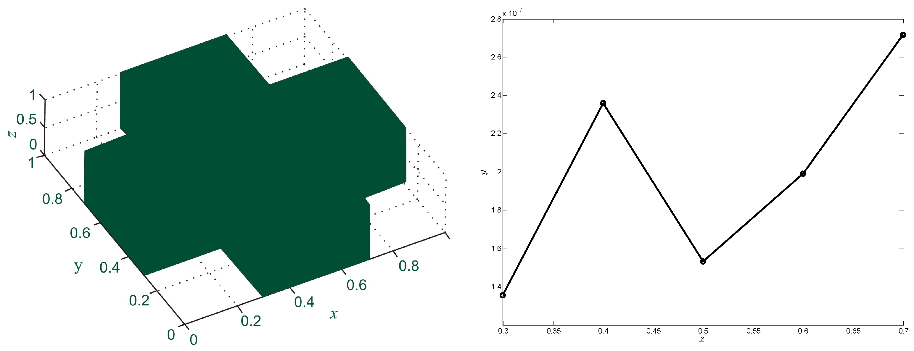
4. Numerical Results

In this section, we apply the SRBF method for the numerical solution of two-dimensional Poisson and Helmholtz and three-dimensional Poisson elliptic PDEs with Dirichlet boundary conditions. We used MQ radial basis functions. The accuracy of the scheme is measured in terms of the error norms L a b s , L , and Root Mean Square error (RMS).
L a b s = | u ( i ) e x u i | , i = 1 , 2 , , N n . L = m a x ( L a b s ) , RMS = i = 1 N ( u i ) 2 N ,
where u e x represents the exact and u represents the approximate solution.
In this paper, the SRBF method is applied on both regular and irregular domains, as well as on uniform and non-uniform (Chebyshev, random, and Halton) nodal points. Numerical results of the paper are summarized as follows. Numerical results of two-dimensional Poisson equations with uniform nodes are shown in Table 1 and Table 2 and in Figure 1 and Figure 2, and those with non-uniform nodes are shown in Figure 3, whereas numerical results over different types of irregular domains are shown in Figure 4, Figure 5, Figure 6, Figure 7 and Figure 8. Numerical results of two-dimensional Helmholtz equations are shown in Table 3 and Table 4 and in Figure 9 and Figure 10. Numerical results of three-dimensional Poisson equations are shown in Table 5 and in Figure 11, Figure 12 and Figure 13.
Problem 1.
Consider the two-dimensional Poisson equation:
u x x + u y y = f ( x , y ) , ( x , y ) [ 1 , 1 ] 2 ,
where function f ( x , y ) is specified so that the exact solution is [23]:
u ( x , y ) = 65 65 + ( x 0.2 ) 2 + ( y + 0.1 ) 2 .
Numerical results in terms of L and RMS for various values of nodes N and corresponding shape parameters value c for Problem 1 are reported in Table 1. One can see that better accuracy is obtained for each N.
Numerical results of the proposed meshless method for N = 256 and c = 0.125 are shown in Figure 1 (left), whereas the L a b s error norm is shown in Figure 1 (right).
Problem 2.
Consider the two-dimensional Poisson equation:
u x x + u y y = 5 / 4 π 2 sin ( π x ) cos ( π y / 2 ) , ( x , y ) [ a , b ] 2 .
The exact solution [7] is given by:
u ( x , y ) = sin ( π x ) cos ( π y / 2 ) .
Numerical results of Problem 2 are obtained using the proposed meshless method, and in this case, the method is analyzed up to the maximum nodes N = 2500 . The L and RMS error norms are calculated for different values of N and the corresponding value of c and are shown in Table 2. It can be observed from the table that the accuracy increases with the increase in the number of nodes.
The proposed method is truly meshless and eliminates the need for meshing. Numerical solutions for N = 400 and c = 0.96 are shown in Figure 2 (left), whereas the L a b s error norm is shown in Figure 2 (right). Figure 3 shows the numerical results in terms of L error norms using random nodes, Chebyshev nodes, and Halton nodes. Figure 3 is the evidence that better accuracy is obtained in these cases, as well.
Numerical results using the SRBF method over different types of irregular domains are shown in Figure 4, Figure 5, Figure 6, Figure 7 and Figure 8. One can see that a better approximate solution can be obtained by the proposed method.
Problem 3.
Consider the two-dimensional Helmholtz equation:
u x x + u y y + k u ( x , y ) = cos ( t x ) sin ( t y ) ( 2 t 2 + k ) , ( x , y ) [ 0 , 1 ] 2 ,
where k = 5 and t is the frequency variable; the exact solution is:
u ( x , y ) = cos ( t x ) sin ( t y ) .
Numerical results for Problem 3 for various frequencies t and nodes N are shown in Table 3. Figure 9 shows the numerical result and absolute error of the proposed method with t = 10, c = 1.22 and N = 400. It can be seen from Figure 9 that reasonably good accuracy can be achieved by the method. Table 3 shows that the proposed method can easily capture the solution up to high frequency at t = 20 . One can also see from the table that accuracy increases with the increase in the number of nodes N in this case as well.
Problem 4.
Consider the two-dimensional Helmholtz equation:
u x x + u y y + k u ( x , y ) = f ( x , y ) , ( x , y ) [ 0 , 1 ] 2 ,
with k = 5 [24], and the function f ( x , y ) is specified, so that the exact solution is:
u ( x , y ) = e x y ( x 2 x ) 2 ( y 2 y ) 2 .
Numerical results for Problem 4 are reported in Table 4 for different N and its corresponding shape parameter value c in terms of L and R M S error norms. Better results are obtained in this case, as well, and the accuracy increases with increase in N. The accuracy of the proposed method is also shown in Figure 10.
Problem 5.
Consider the three-dimensional Poisson equation:
u x x + u y y + u z z = 6 , ( x , y ) [ 0 , 1 ] 2 .
The exact solution is [25]:
u ( x , y , z ) = x 2 + y 2 + z 2 .
To check the efficiency of the SRBF method in the three-dimensional case, we have considered the Poisson equation. The results of Problem 5 are shown in Table 5. The proposed meshless method in the three-dimensional case is also tested over different irregular domains, as shown in Figure 11, Figure 12 and Figure 13. The performance of the method is satisfactory in these cases as well.

5. Conclusions

In this study, we have used the symmetric radial basis function method for the simulation of two- and three-dimensional elliptic PDEs. For this purpose, we have employed uniform and non-uniform nodes. Furthermore, the accuracy of the method has been testified in regular, as well as irregular domains.

Author Contributions

Conceptualization, P.T. and M.N.K.; Data curation, I.H. and I.A.; Formal analysis, P.T. and P.K.; Funding acquisition, P.T. and P.K.; Investigation, M.N.K. and P.K.; Methodology, I.H. and I.A.; Resources, I.H. and I.A.; Supervision, M.N.K. and P.K.; Validation, P.T. and M.N.K.; Visualization, I.H. and I.A.; Writing—review & editing, I.H., I.A., and P.K.

Funding

This research was funded by King Mongkut’s University of Technology, North Bangkok, Grant number No. KMUTNB-61-GOV-D-68.

Acknowledgments

The authors acknowledge the financial support provided by King Mongkut’s University of Technology Thonburi through the “KMUTT 55th Anniversary Commemorative Fund”. This project was supported by the Theoretical and Computational Science (TaCS) Center under the Computational and Applied Science for Smart Innovation Cluster (CLASSIC), Faculty of Science, KMUTT. Moreover, this research work was financially supported by King Mongkut’s University of Technology, North Bangkok, Contract No. KMUTNB-61-GOV-D-68.

Conflicts of Interest

The authors declare no conflict of interest.

References

  1. Graeme, F.; Andreas, K.; Jon, M. Compact optimal quadratic spline collocation methods for the Helmholtz equation. J. Comput. Phys. 2011, 230, 2880–2895. [Google Scholar]
  2. Ali, A.A.; Bernard, B. Modified nodal cubic spline collocation for Poisson’s equation. SIAM J. Numer. Anal. 2008, 46, 397–418. [Google Scholar]
  3. Philippe, C. The Finite Element Method for Elliptic Problems; SIAM: Philadelphia, PA, USA, 2002. [Google Scholar]
  4. Britt, S.; Semyon, T.; Eli, T. A compact fourth order scheme for the Helmholtz equation in polar coordinates. J. Sci. Comput. 2010, 45, 26–47. [Google Scholar] [CrossRef]
  5. Ronald, B. Families of high order accurate discretizations of some elliptic problems. SIAM J. Sci. Stat. Comput. 1981, 2, 268–284. [Google Scholar]
  6. Romina, G.; Renato, S. Comparing Shannon to autocorrelation-based wavelets for solving singularly perturbed elliptic BV problems. BIT Numer. Math. 2012, 52, 21–43. [Google Scholar]
  7. Fasshauer, G.E. Meshfree Approximation Methods with MATLAB; World Scientific: Singapore, 2007; Volume 6. [Google Scholar]
  8. Nam, M.; Thanh, T. An integrated-RBF technique based on Galerkin formulation for elliptic differential equations. Eng. Anal. Bound. Elem. 2009, 33, 191–199. [Google Scholar] [Green Version]
  9. Khan, W.; Ullah, B. Analysis of meshless weak and strong formulations for boundary value problems. Eng. Anal. Bound. Elem. 2017, 80, 1–17. [Google Scholar] [CrossRef]
  10. Siraj-ul-Islam; Ahmad, I. A comparative analysis of local meshless formulation for multi-asset option models. Eng. Anal. Bound. Elem. 2016, 65, 159–176. [Google Scholar] [CrossRef]
  11. Ahmad, I. Local meshless method for PDEs arising from models of wound healing. Appl. Math. Model. 2017, 48, 688–710. [Google Scholar]
  12. Aziz, I.; Ahmad, M. Numerical solution of two-dimensional elliptic PDEs with nonlocal boundary conditions. Comput. Math. Appl. 2015, 69, 180–205. [Google Scholar]
  13. Kansa, E.J. Multiquadrics—A scattered data approximation scheme with applications to computational fluid-dynamics—I surface approximations and partial derivative estimates. Comput. Math. Appl. 1990, 19, 127–145. [Google Scholar] [CrossRef]
  14. Leevan, L.; Roland, O.; Robert, S. Results on meshless collocation techniques. Eng. Anal. Bound. Elem. 2006, 30, 247–253. [Google Scholar] [Green Version]
  15. Damian, B.; Leevan, L.; Kansa, E.; Jermy, L. On approximate cardinal preconditioning methods for solving PDEs with radial basis functions. Eng. Anal. Bound. Elem. 2005, 29, 343–353. [Google Scholar]
  16. Fasshauer, G.E. Solving partial differential equations by collocation with radial basis functions. In Surface Fitting and Multiresolution Methods, 1st ed.; Vanderbilt University Press: Nashville, TN, USA, 1997; pp. 1–8. [Google Scholar]
  17. Wu, Z. Hermite-Birkhoff interpolation of scattered data by radial basis functions. Approx. Theory Its Appl. 1992, 8, 1–10. [Google Scholar]
  18. Robert, S. Multivariate interpolation and approximation by translates of a basis function. Ser. Approx. Decompos. 1995, 6, 491–514. [Google Scholar]
  19. Bartur, J.; Sia, A.; Ke, C. The Hermite collocation method using radial basis functions. Eng. Anal. Bound. Elem. 2000, 24, 607–611. [Google Scholar]
  20. Rocca, L.; Hernandez, R.A.; Power, H. Radial basis function Hermite collocation approach for the solution of time dependent convection–diffusion problems. Eng. Anal. Bound. Elem. 2005, 29, 359–370. [Google Scholar] [CrossRef]
  21. David, S.; Power, H.; Michael, L.; Herve, M. A meshless solution technique for the solution of 3D unsaturated zone problems, based on local Hermitian interpolation with radial basis functions. Transp. Porous Media 2009, 79, 149–169. [Google Scholar]
  22. David, S.; Power, H.; Herve, M. An order-N complexity meshless algorithm for transport-type PDEs, based on local Hermitian interpolation. Eng. Anal. Bound. Elem. 2009, 33, 425–441. [Google Scholar]
  23. Scott, S.; Kansa, E.J. Multiquadric radial basis function approximation methods for the numerical solution of partial differential equations. Adv. Comput. Mech. 2009, 2, 1–206. [Google Scholar]
  24. Aziz, I.; Šarler, B. Wavelets collocation methods for the numerical solution of elliptic Boundary Value problems. Appl. Math. Model. 2013, 37, 676–694. [Google Scholar] [CrossRef]
  25. Alemayehu, S.; Chand, M.R. An efficient direct method to solve the three dimensional Poisson’s equation. Am. J. Comput. Math. 2011, 1, 285. [Google Scholar]
Figure 1. Numerical approximation (left) and L a b s error norm (right) for Problem 1 for N = 256.
Mathematics 06 00327 g001
Figure 2. Numerical approximation (left) and L a b s error norm (right) for Problem 2 for N = 400.
Mathematics 06 00327 g002
Figure 3. L error norm with different non-uniform nodes for Problem 2. (a) Chebyshev nodes N = 100 ; (b) L error norm using Chebyshev nodes; (c) random nodes N = 100 ; (d) L error norm using random nodes; (e) Halton nodes N = 107 ; (f) L error norm using Halton nodes.
Mathematics 06 00327 g003aMathematics 06 00327 g003b
Figure 4. Computational domain x-axis [ 1 , 1 ] and y-axis [ 1 , 1 ] (left) and numerical solution (right) for Problem 2.
Mathematics 06 00327 g004
Figure 5. Computational domain x-axis [ 2.5 , 2.5 ] and y-axis [ 2.5 , 2.5 ] (left) and numerical solution (right) for Problem 2.
Mathematics 06 00327 g005
Figure 6. Computational domain x-axis [ 2 , 2 ] and y-axis [ 2 , 2 ] (left) and numerical solution (right) for Problem 2.
Mathematics 06 00327 g006
Figure 7. Computational domain x-axis [ 3 , 3 ] and y-axis [ 3 , 3 ] (left) and numerical solution (right) for Problem 2.
Mathematics 06 00327 g007
Figure 8. Computational circle domain x-axis [ 3 , 3 ] and y-axis [ 3 , 3 ] (left) and numerical solution (right) for Problem 2.
Mathematics 06 00327 g008
Figure 9. Numerical approximation (left) and L a b s error norm (right) for Problem 3 for N = 400.
Mathematics 06 00327 g009
Figure 10. Numerical approximation (left) and L a b s error norm (right) for Problem 4 for N = 1600.
Mathematics 06 00327 g010
Figure 11. A three-dimensional computational domain for Problem 5.
Mathematics 06 00327 g011
Figure 12. Computational domain (left) and L a b s error norm on the line x = y = z (right) for Problem 5.
Mathematics 06 00327 g012
Figure 13. Computational domain (left) and L a b s error norm on the line x = y = z (right) for Problem 5.
Mathematics 06 00327 g013
Table 1. Error norms for Problem 1.
Nc L RMS
810.124 1.6296 × 10 11 4.4250 × 10 11
2560.125 6.1207 × 10 11 2.3986 × 10 11
4000.125 4.6252 × 10 11 2.8510 × 10 10
9000.129 1.6221 × 10 10 1.3108 × 10 9
16000.126 8.8824 × 10 11 1.4803 × 10 9
25000.126 2.5943 × 10 10 2.9648 × 10 9
Table 2. Error norms for Problems 2.
Nc L RMS
810.406 5.3081 × 10 7 1.5419 × 10 6
2560.52 3.1206 × 10 7 1.1868 × 10 6
4000.96 5.3085 × 10 8 3.0250 × 10 7
9001.67 2.3015 × 10 8 2.6587 × 10 7
16002.15 2.1188 × 10 8 3.7525 × 10 7
25002.52 1.4109 × 10 8 4.6924 × 10 7
Table 3. Error norms for Problem 3.
tNc L RMS
1810.3 5.0926 × 10 8 1.3014 × 10 7
4000.8 1.5166 × 10 8 8.7744 × 10 8
9001.59 4.9779 × 10 9 3.4086 × 10 8
5810.43 7.7247 × 10 5 1.8988 × 10 4
4001.1 7.5979 × 10 7 3.6823 × 10 6
9001.69 1.7120 × 10 7 9.8686 × 10 7
10811.15 1.8200 × 10 2 3.7200 × 10 2
4001.22 1.5067 × 10 5 6.9115 × 10 5
9001.93 4.1883 × 10 8 2.5267 × 10 5
20814.13 2.4950 × 10 1 4.4920 × 10 1
4001.97 2.9000 × 10 3 8.2000 × 10 3
9002.22 1.2416 × 10 4 5.4952 × 10 4
Table 4. Error norms for Problem 4.
Nc L RMS
810.73 8.5033 × 10 6 2.2291 × 10 5
2560.9 3.5236 × 10 7 1.8206 × 10 6
4001.31 7.2561 × 10 8 4.5238 × 10 7
9002.02 1.8554 × 10 8 1.4499 × 10 7
16002.42 4.5357 × 10 9 4.9253 × 10 8
25002.92 1.9209 × 10 9 1.5399 × 10 8
Table 5. Error norms for Problem 5.
Nc L RMS
3430.06 3.6458 × 10 6 1.7514 × 10 5
13310.06 3.7429 × 10 6 2.9703 × 10 5
33750.06 5.1290 × 10 6 6.9616 × 10 5

