A Meshless Method for Burgers’ Equation Using Multiquadric Radial Basis Functions With a Lie-Group Integrator

Abstract

An efficient technique is proposed to solve the one-dimensional Burgers’ equation based on multiquadric radial basis function (MQ-RBF) for space approximation and a Lie-Group scheme for time integration. The comparisons of the numerical results obtained for different values of kinematic viscosity are made with the exact solutions and the reported results to demonstrate the efficiency and accuracy of the algorithm. It is shown that the numerical solutions concur with existing results and the proposed algorithm is efficient and can be easily implemented.

1. Introduction

We consider the nonlinear Burgers’ equation in the one-dimensional case

$$\frac{\partial u(x,t)}{\partial t}+\frac{\partial }{\partial x}F\left(u(x,t)\right)=v\frac{{\partial }^{2}u\left(x,t\right)}{\partial x^2}$$

(1)

with initial condition

$$u\left(x,0\right)=u_0\left(x\right),a\le x\le b$$

and boundary conditions

$$u\left(a,t\right)=h_1\left(t\right),u\left(b,t\right)=h_2\left(t\right),0\le t$$

(2)

where, $F\left(u\left(x,t\right)\right)=\frac{1}{2}u{\left(x,t\right)}^2$, $v>0$ is interpreted as kinematic viscosity number and $u_0\left(x\right)$, $h_1\left(t\right)$, $h_2\left(t\right)$ are known sufficiently smooth functions of the time and space variables, respectively. The steady solutions of the Burgers’ equation, for the first time, are presented by Bateman [1]. Burger [2] proposed this equation as a model of turbulence. The Burgers equation is considered to be a simplified model of the Navier-Stokes equation because they share common nonlinear and viscosity terms. Additionally, it may be helpful to understand the physical mechanisms of the wave motion from advection and dissipation terms. The analytical solutions in the terms of infinite series can be computed by using the Hopf-Cole transformation [3,4] and this gives the opportunity for a comparison between numerical algorithms. Throughout history, there have been many investigations of Burgers’ equation in a variety of different areas including nonlinear wave, shock waves, traffic flows, gas dynamics, elasticity, etc. (see [5] and references therein). For all these reasons, Burgers’ equation has been dealt with by many researchers. The authors of [6] examined different exact solutions of the one-dimensional Burgers’ equation. Many researchers approximate the solutions of the Burgers’ equation by various numerical schemes such as finite difference, finite element, exponentially fitted, Haar wavelet, differential quadrature [7,8,9,10,11].

A kind of univariate multiquadric (MQ) quasi-interpolation technique to approximate a solution of the Burgers’ equation is tailored by Chen and Zu [12]. A meshless method of lines based on radial basis functions (RBFs) is proposed for the numerical solution of Burgers’-type equations in [13]. Xie et al. [14] presented the method of particular solutions based on RBFs and finite difference scheme to solve one-dimensional time-dependent inhomogeneous Burgers’ equations. Two mesh-free methods, in which the MQ quasi-interpolation method is applied in direct and indirect forms for the numerical solution of the Burgers’ equation, are proposed in [15]. Fan et al. [16] developed a mesh-free numerical method based on a combination of the multiquadric RBFs (LRBFCM) and the fictitious time integration method (FTIM) to solve the two-dimensional Burgers’ equations. Bouhamidi et al. [17] presented RBFs interpolation technique for spatial discretization and implicit Runge–Kutta (IRK) schemes for temporal discretization of the unsteady coupled Burgers’-type equations. Xie et al. [18] approximated the solution of the Burgers’ equation spatially by the multiquadric MQ-RBF and used C-N finite difference scheme as temporal discretization technique.

On the other hand, the goal of Geometric Numerical Integration (GNI) is to preserve geometric structure of the systems when approximating their solutions. Thus, the discretized solution of the differential equation has the same qualitative properties of the system [19,20]. Lie-group methods are a class of geometric numerical integrators which preserve qualititative structure of the exact solution. Thus, one can preserve the structural properties of the true flows [21]. The authors of [22] presented a group preserving scheme based on Cayley transformation for Burgers’ equation, in which finite difference method is used for spatial discretization. Furthermore, a combination of the one-step backward group preserving scheme (BGPS) and the numerical method of line to discretize the time and spatial variables, respectively, is presented in [23] to solve Burgers’ equation numerically.

In the present work, the numerical solutions of the one-dimensional Burgers’ equation is analyzed by the MQ-RBFs and a Lie-Group version of Euler method for space and temporal discretization technique, respectively. The goal is to take advantage of both meshless method and GNI method for numerical approximations obtained by this combination of the Lie-Group method based on radial basis functions (LG-RBFs). This method has been recently applied to the Heat equation [24] and high-dimensional generalized Benjamin-Bona-Mahony-Burgers’ equation [25].

2. Numerical Scheme

In this section, we introduce a scheme which consists of the MQ-RBFs and the first-order explicit Lie-group version of Euler method to solve Burgers’ equation numerically.

2.1. The Multiquadric Radial Basis Approximation

We approximate Burgers’ equation spatially by the MQ-RBFs to obtain a nonlinear system of ordinary differential equations. The approximation of the function $u(x,t$) can be written as

$$u\left(x,t\right)\approx \sum _{j=1}^M{\lambda }_j\left(t\right)\phi \left(r_j\right)+{\lambda }_{M+1}\left(t\right)x+{\lambda }_{M+2}\left(t\right),$$

(3)

where the MQ-RBFs defined as

$$\phi \left(x\right)=\phi \left(r_j\right)=\sqrt{r_j^2+c^2},$$

(4)

where $r_j=∥x-x_j∥$ is the Euclidean norm and the unknown functions ${\lambda }_j\left(t\right)$’s can be determined by the collocation technique [26,27]. The number c appeared in Formula (4) interpreted as a shape parameter and it plays an important role in the accuracy of the schemes. One can control the shape of RBFs with the free parameter c. Thus, the selection of its appropriate value is very important to minimize the error of approximation. Mostly authors use "trial and error" to describe an acceptable value of shape parameter for highly accurate results. We also follow the same technique to compute shape parameters for experiments. However, collocating (3) at the M points yields the M equations, an extra two equations are required. This is assured by considering additional two conditions for (3) given as [27]

$$\sum _{j=1}^M{{\lambda }_j}^n=\sum _{j=1}^M{{\lambda }_j}^n{x}_j=0,$$

(5)

where ${{\lambda }_j}^n={\lambda }_j\left(t_n\right).$ Following [25], one can write

$$\phi \left(r_{ij}\right)=\sqrt{{(x_i-x_j)}^2+c^2},$$

where the collocation points $\left\{x_i\right\}$ on the interval [a, b] are called for $2\le i\le M-2$ as center points and for $i=1$ and $i=M$ as boundary points. If one inserts Equation (3) for $2\le i\le M-2$ into Equation (1) then obtains following nonlinear system of differential equations

$$\frac{d}{dt}u\left(t\right)=f(t,u\left(t\right)),$$

(6)

where

$$u\left(t\right)={\left[\sum _{j=1}^M{\lambda }_j\left(t\right)\phi \left(r_{ij}\right)+{\lambda }_{M+1}\left(t\right)+{\lambda }_{M+2}\left(t\right)\right]}_{i=2}^{i=M-1},$$

(7)

and

$$\begin{array}{cc}\hfill f(t,u\left(t\right))=[& \nu \sum _{j=1}^M{\lambda }_j\left(t\right)\frac{{\partial }^2\phi \left(r_{ij}\right)}{\partial x^2}\hfill \\ \hfill & -\frac{\partial }{\partial x}F(\sum _{j=1}^M{\lambda }_j\left(t\right)\phi \left(r_{ij}\right)+{\lambda }_{M+1}\left(t\right)x+{\lambda }_{M+2}\left(t\right)){]}_{i=2}^{i=M-1}.\hfill \end{array}$$

(8)

2.2. Lie-Group Method

We have used Lie-group version of Euler method as a temporal approximation scheme to solve the system of ordinary differential Equation (6) numerically. Using Equation (6) one has

$$\frac{d}{dt}∥u∥=\frac{f.u}{\parallel u\parallel }.$$

(9)

Merging Equations (6) and (9) leads to a system of differential equations

$$\frac{dt}{d}U=AU,$$

(10)

where

$$U=\left[\begin{array}{c}u\\ ∥u∥\end{array}\right],$$

is an augmented vector,

$$A=\left[\begin{array}{cc}{0}_{d\times d}& \frac{f(t,u)}{∥u∥}\\ \frac{f^T(t,u)}{∥u∥}& 0\end{array}\right],$$

(11)

is an augmented matrix of state variables [28]. Notice that the first equation in (10) is the same as Equation (6) and the second one is known as Minkowskian structure for the augmented system. The augmented vector U verifies the cone condition

$$U^{T}gU=u.u-{∥u∥}^2={∥u∥}^2-{∥u∥}^2=0,$$

(12)

where Minkowski metric g is defined as

$$g=\left[\begin{array}{cc}{I}_{d\times d}& 0_{d\times 1}\\ 0_{1\times d}& -1\end{array}\right],$$

$d\times d$ identity matrix given with $I_{d\times d}$ and the dot between two d-dimensional vectors defines the Euclidean inner product [28]. Furthermore, the matrix A defined by (11) belongs to the Lie algebra of the Lorentz group $S{O}_0(d,1)$, i.e.,

$$A^{T}g+gA=0.$$

Now we have extended $(d+1)$-dimensional system (10) of the d-dimensional system (6), which has the additional property that the solutions should satisfy cone condition (12). Thus, it is very important to preserve this property by the numerical integrators. All one must do is to check the properties

$$G^{T}gG=g,$$

$$detG=1,$$

$$G_0^0>0,$$

with $G\left(t_n\right)\in S{O}_0(d,1)$

$$U_{n+1}=G\left(t_n\right)U_n,$$

(13)

where $U_n\approx U\left(t_n\right)$ and $G_0^0$ is the zeroth component of G [28]. A Lie-group version of first-order Euler method can be applied to solve Equation (10) as follows

$$U_{n+1}=\exp (\Delta tA\left(t_n\right))U_n,$$

where $U_{n+1}\in S{O}_0(d,1)$. On the other hand, it is easy to express $\exp (\Delta tA\left(t_n\right))$ in closed-form

$$\exp (\Delta tA\left(t_n\right))=\left[\begin{array}{cc}{I}_n+\frac{(a_n-1)}{{∥f_n∥}^2}{f}_n{f}_n^T& \frac{b_n{f}_n}{∥f_n∥}\\ \frac{b_n{f}_n^T}{∥f_n∥}& a_n\end{array}\right],$$

where, $u_n\approx u\left(t_n\right)$, $\Delta t=t_{n+1}-t_n$, $f_n=f(u_n,t_n)$ and

$$\begin{array}{c}\hfill a_n=\cos \mathrm{h}\left(\frac{\Delta t∥f_n∥}{∥u_n∥}\right),b_n=\sin \mathrm{h}\left(\frac{\Delta t∥f_n∥}{∥u_n∥}\right).\end{array}$$

Inserting this expression of $\exp (\Delta tA\left(t_n\right))$ for $G\left(t_n\right)$ into (13) gives

$$\begin{array}{cc}\hfill u_{n+1}& =u_n+{\zeta }_n{f}_n,\hfill \end{array}$$

(14)

$$\begin{array}{cc}\hfill {\zeta }_n& =\frac{(a_n-1)f_n.u_n+b_n∥u_n∥∥f_n∥}{{∥f_n∥}^2}\hfill \end{array}$$

(15)

$$\begin{array}{cc}\hfill ∥u_{n+1}∥& =\frac{b_n(f_n.u_n)+a_n∥u_n∥∥f_n∥}{∥f_n∥}.\hfill \end{array}$$

(16)

The Equations (14)–(16) preserve the cone condition for each advanced time. Furthermore, the scheme (14) unconditionally preserves the fixed point and the geometric property of the true flows of the original equation (see [25], Theorem 1,2).

Now we apply scheme (14) to solve Equation (6) given with Equations (7)–(8). Let

$$t_n=n\Delta t,n=0,\dots ,N$$

be discrete time points with steplength $\Delta t=T/N$. If one considers scheme (14) for $n=0$ at initial time $t_0=0$ then has

$$\sum _{j=1}^M{\lambda }_j^1\phi \left(r_{ij}\right)+{\lambda }_{M+1}^1{x}_i+{\lambda }_{M+2}^1=u_0\left(x_i\right)+{\zeta }_0{f}_0,i=2,\dots ,M-1,$$

where $f_0={\left[u_0^{{}^{″}}\left(x_i\right)-F^{\prime }\left(u_0\left(x_i\right)\right)\right]}_{i=2}^{M-1}$ and ${\zeta }_0$ can be computed from Equation (15). For $1\le n\le N-1$, $i=2,\dots ,M-1$ one has

$$\sum _{j=1}^M{\lambda }_j^{n+1}\phi \left(r_{ij}\right)+{\lambda }_{M+1}^{n+1}{x}_i+{\lambda }_{M+2}^{n+1}=\sum _{j=1}^M{\lambda }_j^n\phi \left(r_{ij}\right)+{\lambda }_{M+1}^n{x}_i+{\lambda }_{M+2}^n+{\zeta }_n{f}_n,$$

(17)

where

$$f_n={\left[v\sum _{j=1}^M{\lambda }_j^n\frac{{\partial }^2\phi \left(r_{ij}\right)}{\partial x^2}-\frac{\partial }{\partial x}F(\sum _{j=1}^M{\lambda }_j^n\phi \left(r_{ij}\right)+{\lambda }_{M+1}^{n}x+{\lambda }_{M+2}^n)\right]}_{i=2}^{i=M-1},$$

(18)

and ${\zeta }_n$ can be computed from Equation (15). One can write Equations (5), (17), (18) and boundary conditions (2) in the matrix form as follows

$$D{\lambda }^{n+1}=B^{n+1}$$

(19)

where

$$D=\left[\begin{array}{cccccc}\phi \left(r_{11}\right)& \phi \left(r_{12}\right)& \dots & \phi \left(r_{1M}\right)& x_1& 1\\ \phi \left(r_{21}\right)& \phi \left(r_{22}\right)& \dots & \phi \left(r_{2M}\right)& x_2& 1\\ ⋮& ⋮& \ddots & ⋮& ⋮& ⋮\\ \phi \left(r_{M1}\right)& \phi \left(r_{M2}\right)& \dots & \phi \left(r_{MM}\right)& x_M& 1\\ x_1& x_2& \dots & x_M& 0& 0\\ 1& 1& \dots & 1& 0& 0\end{array}\right],$$

$${\lambda }^{n+1}={\left[{\lambda }_1^{n+1},{\lambda }_2^{n+1},\dots ,{\lambda }_M^{n+1},{\lambda }_{M+1}^{n+1},{\lambda }_{M+2}^{n+1}\right]}^T,$$

and

$$B^{n+1}={\left[b_1^{n+1},b_2^{n+1},\dots ,b_M^{n+1},0,0\right]}^T.$$

Each elements of vector B can be computed for $i=2,\dots ,M-1$ as

$$\begin{array}{cc}\hfill b_i^1& =u_0\left(x_i\right)+{\zeta }_0{f}_0,\hfill \\ \hfill b_i^{n+1}& =\sum _{j=1}^M{\lambda }_j^n\phi \left(r_{ij}\right)+{\lambda }_{M+1}^n{x}_i+{\lambda }_{M+2}^n+{\zeta }_n{f}_n,n=1,\dots ,N-1,\hfill \end{array}$$

and for $i=1,M$ as $b_1^{n+1}=h_1^{n+1},b_M^{n+1}=h_2^{n+1}$, respectively. The coefficients ${\lambda }_j^{n+1}$ are computed by solving the resulting system of (19) and then the numerical solutions are obtained using them in (3). The matrix D can be shown to be invertible and it is often ill-conditioned. One can determine how accurately to solve system of (19) by considering the conditioning of D. The condition number of this system related to small perturbation in D is defined for any norm $∥.∥$ as

$$\kappa \left(D\right)=∥D∥∥D^{-1}∥.$$

It is possible to lose $lo{g}_{10}\kappa \left(D\right)$ digits through the computational process of the system (19) including ill-conditioned matrix D [29]. To solve ill-posed system (19) we have used Gaussian elimination with partial pivoting. We obtained the solutions by using the standard floating-point arithmetic in our computational algorithm. The shape parameter also plays an important role for the conditioning of the matrix D. One can have high accuracy with smaller value of c for a fixed number of points M and in this case one often faces with the ill-conditioned matrix D. On the other hand, the condition number $\kappa \left(D\right)$ increases with the number of collocation points M for fixed the values of c.

One can investigate the numerical stability of the method of line by Rule of Thumb [30]. If the eigenvalues of the discretized spatial operator, scaled by steplength $\Delta t$, are inside the stability region of Lie-Group version of Euler integrator than the proposed algorithm is convergent.

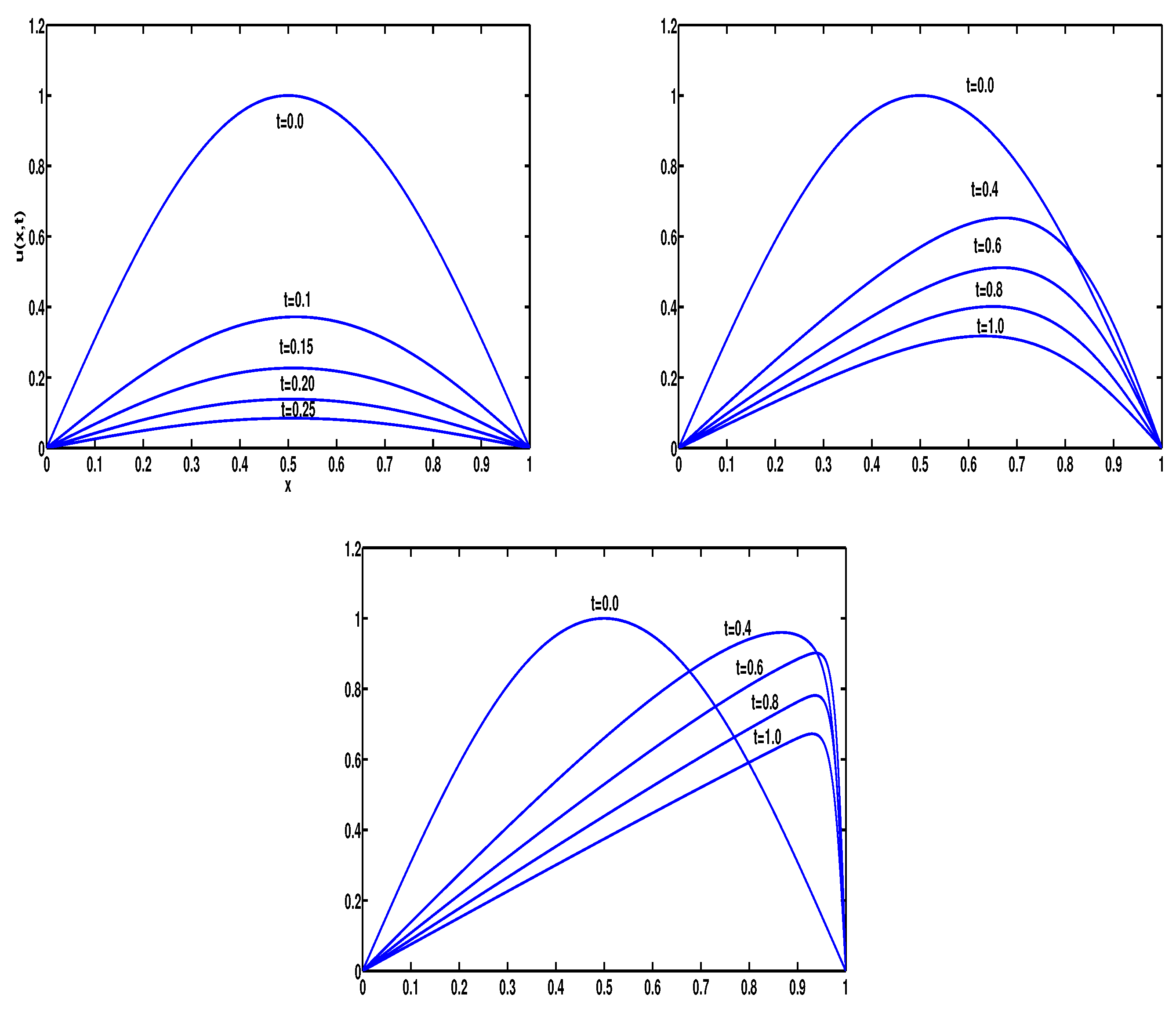
3. Numerical Results

We consider Burgers’ equation on the interval $[0,1]$ with the following initial condition

$$u(x,0)=\sin \left(\pi x\right),$$

and the following boundary conditions

$$u(0,t)=u(1,t)=0,t>0.$$

Its analytical solution is given with the Hopf-Cole transformation as [3,4]

$$u(x,t)=2\nu \pi \frac{{\sum }_{i=1}^{\infty }{k}_i\exp (-i^2{\pi }^2\nu t)i\sin \left(i\pi x\right)}{k_0+{\sum }_{i=1}^{\infty }{k}_i\exp (-i^2{\pi }^2\nu t)\cos \left(i\pi x\right)},$$

(20)

where

$$\begin{array}{cc}\hfill k_0& ={\int }_0^1\exp \left\{-{\left(2\pi \nu \right)}^{-1}\left[1-\cos \left(\pi x\right)\right]\right\}dx,\hfill \\ \hfill k_i& =2{\int }_0^1\exp \left\{-{\left(2\pi \nu \right)}^{-1}\left[1-\cos \left(\pi x\right)\right]\right\}\cos \left(i\pi x\right)dx,\hfill \\ & (i=1,2,3\dots ).\hfill \end{array}$$

We compute the analytical solutions from (20) up to 500 series terms for all comparisons in experiments. The shape parameters are computed by trial and error. We compare the errors for different values of shape parameters which are leading the lower conditioned number of matrix D in (19). We select the shape parameter c for the lowest error values in each experiment. Accuracy of these methods is examined by computing error in $L_2$ and $L_{\infty }$ norm.

$$\begin{array}{cc}\hfill {∥u_{apr}-u∥}_{L_2}& ={\left(h\sum _{j=1}^M{(u_{j,N}-u(x_j,t))}^2\right)}^{1/2},\hfill \\ \hfill {∥u_{apr}-u∥}_{L_{\infty }}& ={\displaystyle \underset{1\le j\le M}{\max }}\left|u_{j,N}-u(x_j,t)\right|.\hfill \end{array}$$

We compute the results of the LG-RBFs for $\nu =1$ at different final times $t=0.1,0.15,0.2,0.25$ with respectively $c=0.299,0.297,0.299,0.299$ and at points $x=0.25,0.5,0.75$. We compare the numerical solutions of the LG-RBFs with GPS [22] for $M=40$, $\Delta t={10}^{-4}$ and with [31] for $M=80$, $\Delta t={10}^{-5}$. The all results tabulated in

Table 1. Comparison of the approximate solution at different final times with $v=1$, $M=40$ and $\Delta t=0.0001$.

x	t	Galerkin [22]	GPS [22]	LG-RBFs	Exact
0.25	0.10	0.25469	0.25376	0.25364	0.25364
	0.15	0.15672	0.15672	0.15660	0.15660
	0.20	0.09619	0.09654	0.09644	0.09644
	0.25	0.05924	0.05929	0.05922	0.05922
0.50	0.10	0.37134	0.37177	0.37157	0.37158
	0.15	0.22674	0.22700	0.22682	0.22682
	0.20	0.13829	0.13862	0.13847	0.13847
	0.25	0.08457	0.08464	0.08454	0.08454
0.75	0.10	0.27102	0.27273	0.27258	0.27258
	0.15	0.16411	0.16450	0.16437	0.16437
	0.20	0.09929	0.09954	0.09943	0.09944
	0.25	0.06036	0.06042	0.06035	0.06035

demonstrate that the LG-RBFs method is highly accurate compared to that of other methods. Now we compute the solutions with LG-RBFs for $\nu =0.1$ at different times $t=0.4,0.6,0.8,1,3$ with respectively $c=0.128,0.312,0.312,0.312$ and at points $x=0.25,0.5,0.75$. Numerical solutions obtained by LG-RBFs with $M=40$, $\Delta t={10}^{-3}$, have been tabulated and compared in

Table 2. Comparison of the approximate solutions at different final times with $v=0.1$, $M=40$ and $\Delta t=0.001$.

x	t	Galerkin [22]	GPS [22]	LG-RBFs	Exact
0.25	0.4	0.31429	0.30889	0.30864	0.30889
	0.6	0.24373	0.24077	0.24061	0.24074
	0.8	0.19758	0.19573	0.19559	0.19568
	1.0	0.16391	0.16264	0.16251	0.16256
	3.0	0.02743	0.02725	0.02720	0.02720
0.50	0.4	0.57636	0.56988	0.56944	0.56963
	0.6	0.45169	0.44745	0.44707	0.44721
	0.8	0.36245	0.35948	0.35914	0.35924
	1.0	0.29437	0.29215	0.29184	0.29192
	3.0	0.04057	0.04028	0.04020	0.04020
0.75	0.4	0.62952	0.62605	0.62564	0.62544
	0.6	0.49034	0.48778	0.48727	0.48721
	0.8	0.37713	0.37438	0.37389	0.37392
	1.0	0.29016	0.28784	0.28741	0.28747
	3.0	0.01334	0.02983	0.02977	0.02977

with exact solution and the numerical solutions presented in [22] for $M=40$, $\Delta t={10}^{-3}$ and [31] for $M=80$, $\Delta t={10}^{-4}$. It is clear from table that LG-RBFs provides accurate results than are obtained by [22,31]. Finally, we compute the solutions with LG-RBFs for $\nu =0.01$ at different times $t=0.4,0.6,0.8,1,3$ with respectively $c=0.121,0.034,0.036,0.114,0.111$ and at points $x=0.25,0.5,0.75$. The results compared in

Table 3. Comparison of the approximate solutions at different final times with $v=0.01$, $M=80$ and $\Delta t=0.0001$.

x	t	Exact-Explicit [7]	RK4 [22]	GPS [22]	LG-RBFs	Exact
0.25	0.4	0.34164	0.34197	0.34193	0.34189	0.34191
	0.6	0.26890	0.26900	0.26897	0.26890	0.26896
	0.8	0.22150	0.22151	0.22149	0.22140	0.22148
	1.0	0.18825	0.18821	0.18820	0.18816	0.18819
	3.0	0.07515	0.07512	0.07511	0.07512	0.07511
0.50	0.4	0.65606	0.66083	0.66079	0.66068	0.66071
	0.6	0.52658	0.52950	0.52946	0.52938	0.52942
	0.8	0.43743	0.43919	0.43916	0.43910	0.43914
	1.0	0.37336	0.37446	0.37443	0.37439	0.37442
	3.0	0.15015	0.15019	0.15018	0.15018	0.15018
0.75	0.4	0.90111	0.91053	0.91058	0.91031	0.91026
	0.6	0.75862	0.76741	0.76739	0.76723	0.76724
	0.8	0.64129	0.64750	0.64747	0.64737	0.64740
	1.0	0.55187	0.55620	0.55609	0.55603	0.55605
	3.0	0.22454	0.22484	0.22483	0.22481	0.22481

with exact solutions and the numerical solutions presented in [7,22,31] with $M=80$, $\Delta t={10}^{-4}$ for all methods. Table 3 indicate that the accuracy of LG-RBFs solutions is compatible with the numerical solutions obtained in [7,22,31]. It is easy to see that the all results tabulated in Tables for the LG-RBFs are in good agreement with the analytical solutions.

We compute $L_2$ and $L_{\infty }$ error norms of the LG-RBFs for $v=1$, $M=10$, $\Delta t=0.001$ at $t=1,2$ with respectively $c=0.588,0.587$ and for $v=0.1$, $M=10$, $\Delta t=0.01$ at $t=3,3.5$ with respectively $0.6,0.611$. We compare these with the error norms of the backward differentiation formula of order one (BDF1) reported in [32]. The results are tabulated for the both first-order schemes (in time) in the

Table 4. Comparison of error norms for different values of final times with $M=10$ and $\Delta t=0.001$.

$\mathit{\nu }=1$	$\mathit{t}=1$		$\mathit{t}=2$
	${\mathit{L}}_{\mathbf{2}}$	${\mathit{L}}_{\infty }$	${\mathit{L}}_{\mathbf{2}}$	${\mathit{L}}_{\infty }$
BDF-1, $M=80$ [32]	1.8457 × 10${}^{-6}$	2.6102 × 10${}^{-6}$	1.9600 × 10${}^{-10}$	2.7713 × 10${}^{-10}$
LG-RBFs	1.1727 × 10${}^{-10}$	1.5587 × 10${}^{-10}$	4.8120 × 10${}^{-14}$	6.7895× 10${}^{-14}$

and

Table 5. Comparison of error norms for different values of final times with $M=10$ and $\Delta t=0.01$.

$\mathit{\nu }=0.1$	$\mathit{t}=3$		$\mathit{t}=3.5$
	${\mathit{L}}_{\mathbf{2}}$	${\mathit{L}}_{\infty }$	${\mathit{L}}_{\mathbf{2}}$	${\mathit{L}}_{\infty }$
BDF-1 [32]	4.2130 × 10${}^{-4}$	5.9753 × 10${}^{-4}$	3.0024 × 10${}^{-4}$	4.2509 × 10${}^{-4}$
LG-RBFs	5.0581 × 10${}^{-5}$	7.1572 × 10${}^{-5}$	3.0291 × 10${}^{-5}$	4.3053 × 10${}^{-5}$

. The tables indicate that the accuracy of LG-RBFs is much better than BDF1 method [32]. It can be seen from Table 4 and Table 5 that the error of LG-RBFs gets smaller than the error of BDF1 method when the final time increases, as we expect. In Figure 1 we show the numerical solutions of the LG-RBFs which are computed for $\nu =1$, $M=40$, $\nu =0.1,0.01$ with $M=80$ and $\Delta t=0.0001$ at different final times, and at $x=0(1/500)1$. The presence of the steep descent can be seen from the Figure 1 for small values of viscosity. Thus, proposed scheme can exhibit the correct physical behavior of the problem.

4. Conclusions

The first-order Lie-Group version of Euler method combined with MQ-RBFs method is proposed to approximate solutions of the one-dimensional Burgers’ equation. The obtained numerical results are compared with analytical and reported results in the literature for a test example at different values of viscosity. It is concluded that the numerical solutions of the proposed scheme are effective in comparison with the analytical and numerical solutions presented in the previous studies. The results show that the presented scheme can capture the nonlinear steep behavior of the Burgers’ equation in the case of smaller values of viscosity. The proposed algorithm can also be used for solving other more general problems.

References

1. Bateman, H. Some recent researches on the motion of fluids. Mon. Weather Rev. 1915, 43, 163–170. [Google Scholar] [CrossRef]
2. Burger, J.M. A mathematical model illustrating the theory of turbulence. Adv. Appl. Math. 1948, 1, 171–199. [Google Scholar] [CrossRef]
3. Cole, J.D. On a quasi-linear parabolic equation in aerodynamics. Q. Appl. Math. 1948, 9, 225–236. [Google Scholar] [CrossRef]
4. Hopf, E. The partial differential equation ut + uux = μuxx. Commun. Pure Appl. Math. 1950, 3, 201–230. [Google Scholar] [CrossRef]
5. Bonkile, M.P.; Awasthi, A.; Lakshmi, C.; Mukundan, V.; Aswin, V.S. A systematic literature review of Burgers’ equation with recent advances. Pramana 2018, 90, 69. [Google Scholar] [CrossRef]
6. Caldwell, J.; Smith, P. Solution of Burgers’ equation with a large Reynolds numbe. Appl. Math. Model. 1982, 6, 381–385. [Google Scholar] [CrossRef]
7. Kutluay, S.; Bahadir, A.R.; Ozdes, A. Numerical solution of one-dimensional Burgers’ equation: Explicit and exact-explicit finite difference methods. J. Comput. Appl. Math. 1999, 103, 251–261. [Google Scholar] [CrossRef]
8. Acedo, L. On the gravitational instability of a set of random walkers. Europhys. Lett. 2006, 73, 698–704. [Google Scholar] [CrossRef]
9. Jiwari, R.; Mittal, R.C.; Sharma, K.K. A umerical scheme based on weighted average differential quadrature method for the numerical solution of Burgers’ equation. Appl. Math. Comput. 2013, 219, 6680–6691. [Google Scholar] [CrossRef]
10. Cordero, A.; Franques, A.; Torregrosa, J.R. Numerical solution of turbulence problems by solving Burgers’ equation. Algorithms 2015, 8, 224–233. [Google Scholar] [CrossRef]
11. Jiwari, R. A hybrid numerical scheme for the numerical solution of the Burgers’ equation. Comput. Phys. Commun. 2015, 188, 59–67. [Google Scholar] [CrossRef]
12. Chen, R.; Wu, Z. Applying multiquadric quasi-interpolation to solve Burgers’ equation. Appl. Math. Comput. 2006, 172, 472–484. [Google Scholar] [CrossRef]
13. Haq, S.; Hussain, A.; Uddin, M. On the numerical solution of nonlinear Burgers’-type equations using meshless method of lines. Appl. Math. Comput. 2012, 218, 6280–6290. [Google Scholar] [CrossRef]
14. Xie, H.; Li, D.; Li, F. A new Numerical Method of Particular Solutions for Inhomogeneous Burgers’ equation. Math. Prob. Eng. 2013. [Google Scholar] [CrossRef]
15. Sarboland, M.; Aminataei, A. On the Numerical Solution of One-Dimensional Nonlinear Nonhomogeneous Burgers’ Equation. J. Appl. Math. 2014. [Google Scholar] [CrossRef]
16. Fan, C.M.; Yang, C.H.; Gu, M.H. Applications of the local RBF collocation method and the fictitious time integration method for Burgers’ equations. Procedia Eng. 2014, 79, 569–574. [Google Scholar] [CrossRef]
17. Bouhamidi, A.; Hached, M.; Jbilou, K. A meshless RBF method for computing a numerical solution of unsteady Burgers’-type equations. Comput. Math. Appl. 2014, 68, 238–256. [Google Scholar] [CrossRef]
18. Xie, H.; Zhou, J.; Jiang, Z.; Guo, X. Approximations for Burgers’ equations with C-N scheme and RBF collocation methods. J. Nonlinear Sci. Appl. 2016, 9, 3727–3734. [Google Scholar] [CrossRef]
19. Hairer, E.; Lubich, C.; Wanner, G. Geometric Numerical Integration: Structure-Preserving Algorithms for Ordinary Differential Equations; Springer: Berlin, Germany, 2006. [Google Scholar]
20. Blanes, S.; Casas, F. A Concise Introduction to Geometric Numerical Integration; CRC Press: New York, NY, USA, 2016. [Google Scholar]
21. Iserles, A.; Munthe-Kaas, H.Z.; Norsett, S.P.; Zanna, A. Lie-group methods. Acta Numer. 2000, 9, 215–365. [Google Scholar] [CrossRef]
22. Liu, C.S. A Group Preserving Scheme for Burgers Equation with Very Large Reynolds Number. CMES 2006, 12, 197–211. [Google Scholar]
23. Liu, C.S. An Efficient Backward Group Preserving Scheme for the Backward in Time Burgers’ Equation. CMES 2006, 12, 5565. [Google Scholar]
24. Hajiketabi, M.; Abbasbandy, S. The combination of meshless method based on radial basis functions with a geometric numerical integration method for solving partial differential equations: Application to the heat equation. Eng. Anal. Bound. Elem. 2018, 87, 36–46. [Google Scholar] [CrossRef]
25. Hajiketabi, M.; Abbasbandy, S.; Casas, F. The Lie-group method based on radial basis functions for solving nonlinear high dimensional generalized Benjamin-Bona-Mahony-Burgers equation in arbitrary domains. Appl. Math. Comput. 2018, 321, 223–243. [Google Scholar] [CrossRef]
26. Kansa, E.J. Multiquadrics—A scattered data approximation scheme with applications to computational fluid dynamics—I surface approximations and partial derivative estimates. Comput. Math. Appl. 1990, 19, 127–145. [Google Scholar] [CrossRef]
27. Kansa, E.J. Multiquadrics—A scattered data approximation scheme with applications to computational fluid dynamics—II solutions to parabolic, hyperbolic and elliptic partial differential equations. Comput. Math. Appl. 1990, 19, 147–161. [Google Scholar] [CrossRef]
28. Liu, C.S. Cone of non-linear dynamical system and group preserving schemes. Int. J. Nonlinear Mech. 2001, 36, 1047–1068. [Google Scholar] [CrossRef]
29. Trefethen, L.N.; Bau, D., III. Numerical Linear Algebra; Siam: Philadelphia, PA, USA, 1997. [Google Scholar]
30. Trefethen, L.N. Spectral Methods in MATLAB; Siam: Philadelphia, PA, USA, 2000. [Google Scholar]
31. Öziş, T.; Aksan, E.N.; Özdeş, A. A finite element approach for solution of Burgers’ equation. Appl. Math. Comput. 2003, 139, 417–428. [Google Scholar] [CrossRef]
32. Mukundan, V.; Awasthi, A. Efficient numerical techniques for Burgers’ equation. Appl. Math. Comput. 2015, 262, 282–297. [Google Scholar] [CrossRef]
Figure 1. Physical behavior of numerical solutions u ( x , t ) for ν = 1 , M = 40 (top left panel) and ν = 0.1 , M = 80 (top right panel) and ν = 0.01 , M = 80 (bottom panel) at different final times for Δ t = 0.0001 .
Mathematics 07 00113 g001