The Space–Time Kernel-Based Numerical Method for Burgers’ Equations


Abstract
1. Introduction
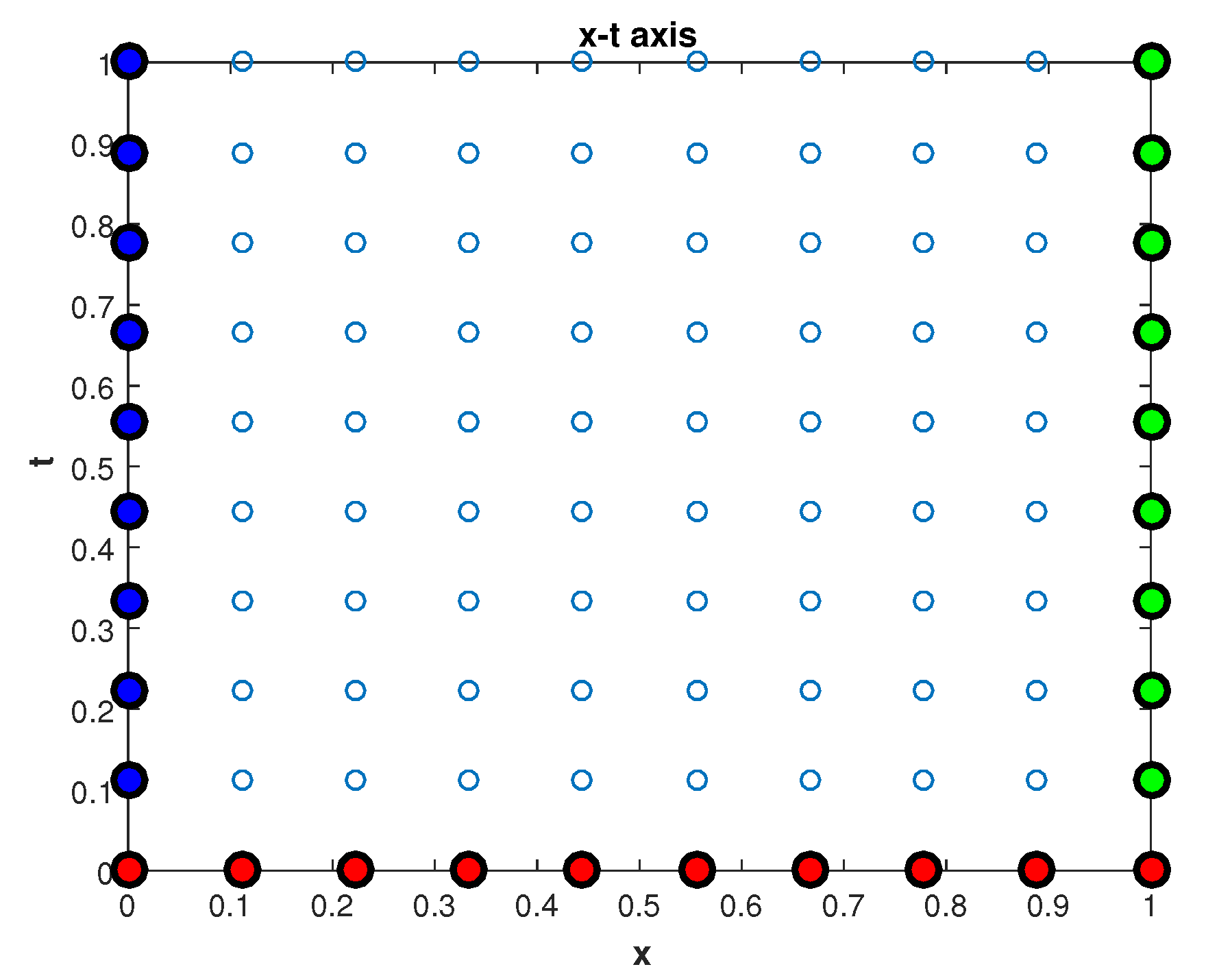
2. Space–Time Kernel-Based Approximation
3. Stability of the Numerical Scheme
4. Numerical Experiments
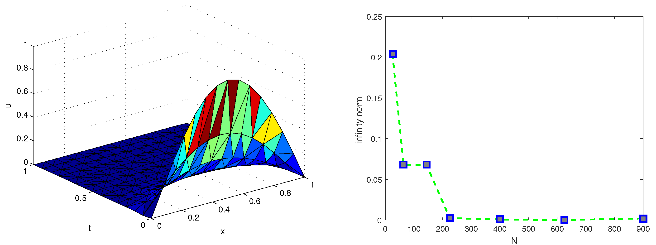
4.1. Example 1
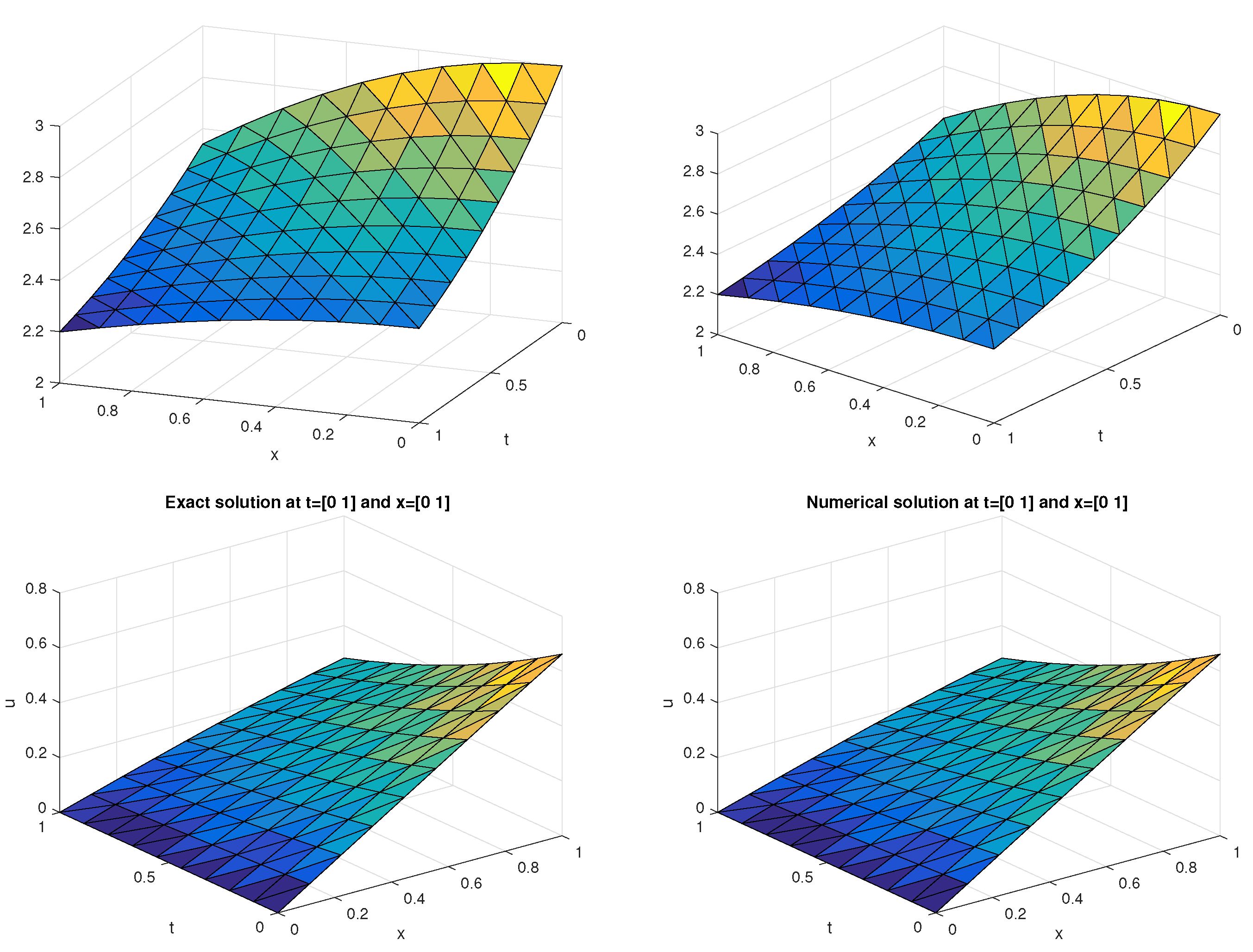
4.2. Example 2
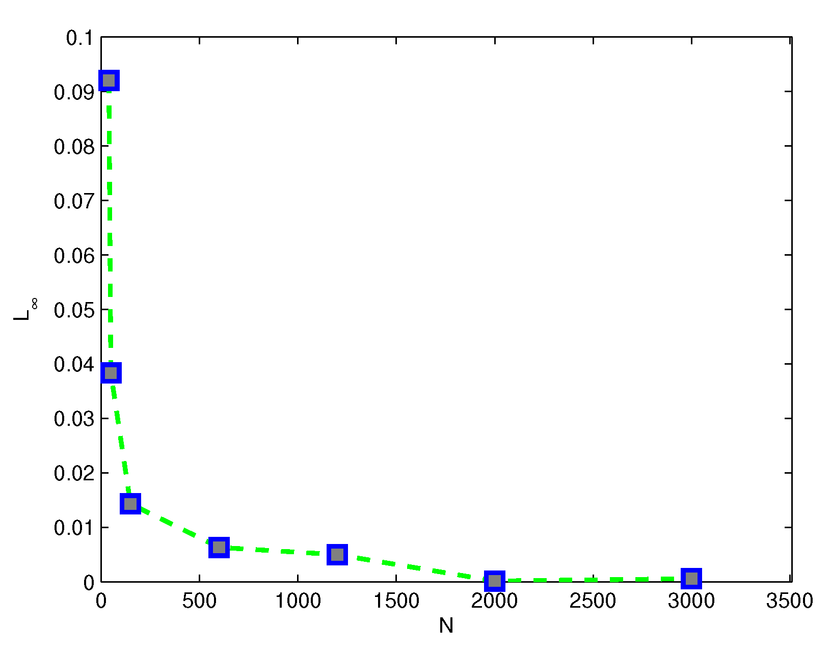
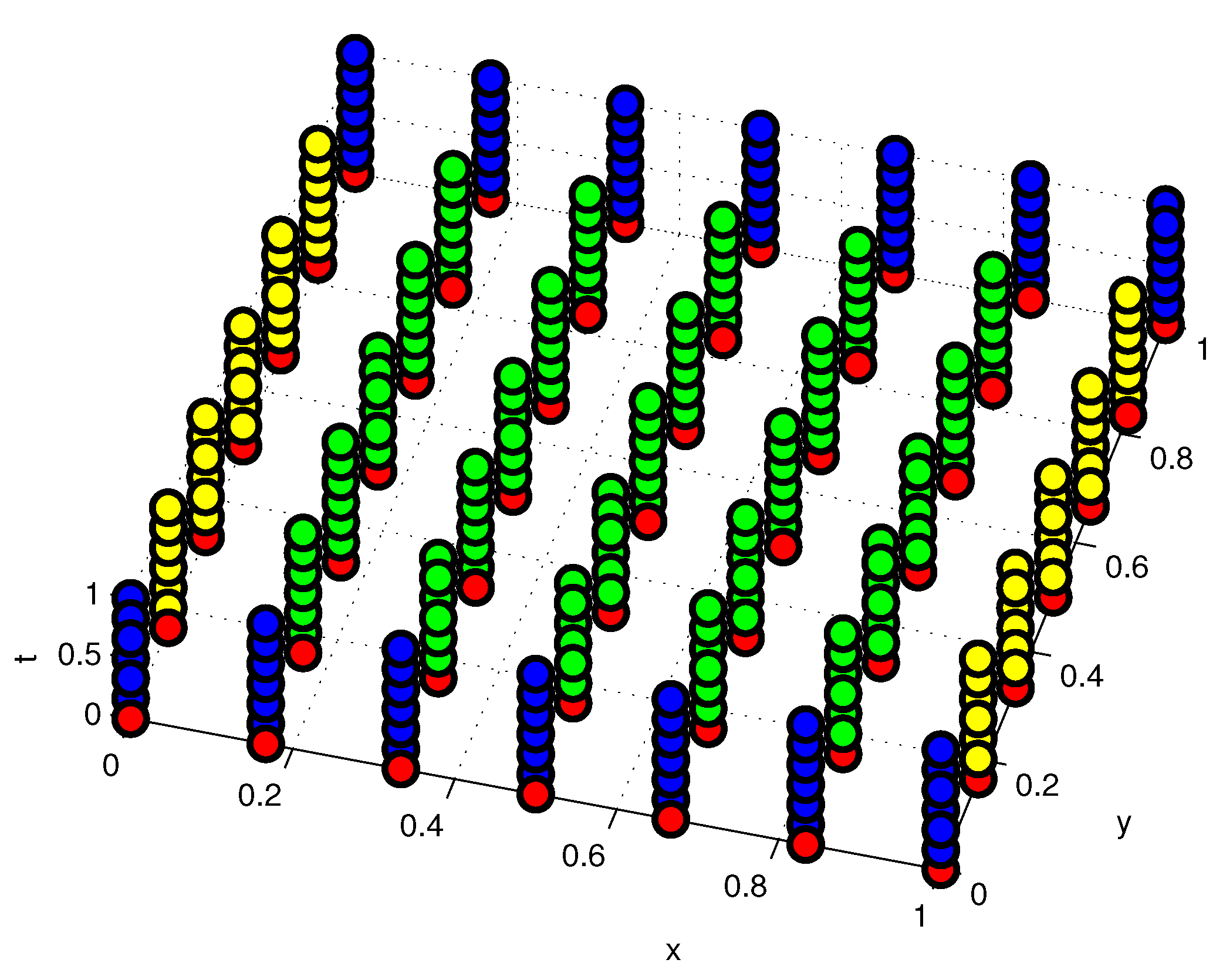
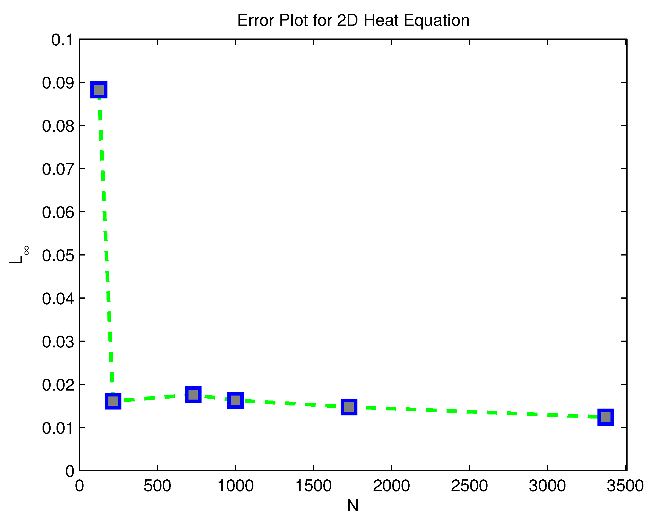
4.3. Example 3
4.4. Concluding Remarks
Author Contributions
Funding
Acknowledgments
Conflicts of Interest
References
- Moukalled, F.; Mangani, L.; Darwish, M. The Finite Volume Method in Computational Fluid Dynamics: An Advanced Introduction with OpenFOAM and Matlab; Springer: Berline Germany, 2016; pp. 3–8. [Google Scholar]
- Sauter, S.A.; Schwab, C. Boundary Element Methods; Springer: Berlin, Germany, 2010; pp. 183–287. [Google Scholar]
- Fasshauer, G.E. Meshfree Approximation Methods with MATLAB; World Scientific: Singapore, 2007; Volume 6. [Google Scholar]
- Cohen, A. Numerical Analysis of Wavelet Methods; Elsevier: Amsterdam, The Netherlands, 2003; Volume 32. [Google Scholar]
- Chen, C.-S.; Karageorghis, A.; Smyrlis, Y.S. The Method of Fundamental Solutions: A Meshless Method; Dynamic Publishers Atlanta: Atlanta, Georgia, 2008. [Google Scholar]
- Canuto, C.; Hussaini, M.Y.; Quarteroni, A.; Zang, T.A. Spectral Methods; Springer: Berlin, Germany, 2006. [Google Scholar]
- Turchetti, C.; Conti, M.; Crippa, P.; Orcioni, S. On the approximation of stochastic processes by approximate identity neural networks. IEEE Trans. Neural Netw. 1998, 9, 1069–1085. [Google Scholar] [CrossRef] [PubMed]
- Turchetti, C.; Crippa, P.; Pirani, M.; Biagetti, G. Representation of nonlinear random transformations by non-Gaussian stochastic neural networks. IEEE Trans. Neural Netw. 2008, 19, 1033–1060. [Google Scholar] [CrossRef] [PubMed]
- Uddin, M.; Kamran, K.; Usman, M.; Ali, A. On the Laplace-transformed-based local meshless method for fractional-order diffusion equation. Int. J. Comput. Methods Eng. Sci. Mech. 2018, 19, 1–5. [Google Scholar] [CrossRef]
- Netuzhylov, H. A Space-Time Meshfree Collocation Method for Coupled Problems on Irregularly-Shaped Domains. Ph.D. Thesis, TU Braunschweig, Braunschweig, Germany, 2008. [Google Scholar]
- Li, Z.; Mao, X. Global multiquadric collocation method for groundwater contaminant source identification. Environ. Model. Softw. 2011, 26, 1611–1621. [Google Scholar] [CrossRef]
- Li, Z.; Mao, X. Global space–time multiquadric method for inverse heat conduction problem. Int. J. Numer. Methods Eng. 2011, 85, 355–379. [Google Scholar] [CrossRef]
- Li, M.; Chen, W.; Chen, C.S. The localized RBFs collocation methods for solving high dimensional PDEs. Eng. Anal. Bound. Elements 2013, 37, 1300–1304. [Google Scholar] [CrossRef]
- Tezduyar, T.E.; Sathe, S.; Keedy, R.; Stein, K. Space–time finite element techniques for computation of fluid–structure interactions. Comput. Methods Appl. Mech. Eng. 2006, 195, 2002–2027. [Google Scholar] [CrossRef]
- Klaij, C.M.; van der Vegt, J.J.W.; van der Ven, H. Space–time discontinuous Galerkin method for the compressible Navier–Stokes equations. J. Comput. Phys. 2006, 217, 589–611. [Google Scholar] [CrossRef]
- Sudirham, J.J.; van der Vegt, J.J.W.; van Damme, R.M.J. Space–time discontinuous Galerkin method for advection–diffusion problems on time-dependent domains. Appl. Numer. Math. 2006, 56, 1491–1518. [Google Scholar] [CrossRef]
- Ambati, V.R.; Bokhove, O. Space–time discontinuous Galerkin finite element method for shallow water flows. J. Comput. Appl. Math. 2007, 204, 452–462. [Google Scholar] [CrossRef]
- Young, D.L.; Tsai, C.C.; Murugesan, K.; Fan, C.M.; Chen, C.W. Time-dependent fundamental solutions for homogeneous diffusion problems. Eng. Anal. Bound. Elements 2004, 28, 1463–1473. [Google Scholar] [CrossRef]
- Fasshauer, G.; McCourt, M. Kernel-Based Approximation Methods Using Matlab; World Scientific Publishing Company: Singapore, 2015; Volume 19. [Google Scholar]
- Hamaidi, M.; Naji, A.; Charafi, A. Space–time localized radial basis function collocation method for solving parabolic and hyperbolic equations. Eng. Anal. Bound. Elements 2016, 67, 152–163. [Google Scholar] [CrossRef]
- Hopf, E. The partial differential equation ut + uux = μxx. Commun. Pure Appl. Math. 1950, 3, 201–230. [Google Scholar] [CrossRef]
- Fasshauer, G.E.; Zhang, J.G. On choosing “optimal” shape parameters for RBF approximation. Numer. Algorithms 2007, 45, 345–368. [Google Scholar] [CrossRef]
- Uddin, M. On the selection of a good value of shape parameter in solving time-dependent partial differential equations using RBF approximation method. Appl. Math. Model. 2014, 38, 135–144. [Google Scholar] [CrossRef]
- Cole, J.D. On a quasi-linear parabolic equation occurring in aerodynamics. Q. Appl. Math. 1951, 9, 225–236. [Google Scholar] [CrossRef]
- Kutluay, S.; Bahadir, A.R.; Özdeş, A. Numerical solution of one-dimensional Burgers equation: Explicit and exact-explicit finite difference methods. J. Comput. Appl. Math. 1999, 103, 251–261. [Google Scholar] [CrossRef]
- Vaganan, B.M.; Priya, E.E. Generalized Cole–Hopf transformations for generalized Burgers equations. Pramana 2015, 85, 861–867. [Google Scholar] [CrossRef]


| Space–Time Solution | Exact Solution | [25] | |||
|---|---|---|---|---|---|
| 0.1 | 0.1548 | 0.1105 | 0.109 | 0.1095 | 0.10954 |
| 0.2 | 0.2084 | 0.2113 | 0.2099 | 0.2098 | 0.20979 |
| 0.3 | 0.2915 | 0.2942 | 0.2925 | 0.2919 | 0.29190 |
| 0.4 | 0.3440 | 0.3502 | 0.3487 | 0.3479 | 0.34792 |
| 0.5 | 0.3753 | 0.3737 | 0.3723 | 0.3716 | 0.37158 |
| 0.6 | 0.3224 | 0.3608 | 0.3597 | 0.3591 | 0.35905 |
| 0.7 | 0.3022 | 0.3112 | 0.3104 | 0.3099 | 0.30991 |
| 0.8 | 0.2259 | 0.2283 | 0.2284 | 0.2278 | 0.22782 |
| 0.9 | 0.1261 | 0.1206 | 0.1215 | 0.1207 | 0.12069 |
| N | C.time | ||||
|---|---|---|---|---|---|
| 5 | 10 | 50 | 3.83 | 5.63 | 0.1213 |
| 10 | 15 | 150 | 1.43 | 2.93 | 0.1757 |
| 20 | 30 | 600 | 6.30 | 1.70 | 2.3641 |
| 30 | 40 | 1200 | 4.97 | 1.24 | 6.2123 |
| 40 | 50 | 2000 | 1.50 | 3.90 | 13.545 |
| 50 | 60 | 3000 | 5.73 | 3.41 | 20.102 |
| N | L | L2 | C.time |
|---|---|---|---|
| 125 | 8.82 | 1.60 | 0.002791 |
| 216 | 1.61 | 4.49 | 0.005528 |
| 729 | 1.76 | 7.11 | 0.070214 |
| 1000 | 1.63 | 7.67 | 0.15588 |
| 1728 | 1.48 | 8.42 | 0.48465 |
| 3375 | 1.24 | 8.93 | 2.0845 |
© 2018 by the authors. Licensee MDPI, Basel, Switzerland. This article is an open access article distributed under the terms and conditions of the Creative Commons Attribution (CC BY) license (http://creativecommons.org/licenses/by/4.0/).
Share and Cite
Uddin, M.; Ali, H. The Space–Time Kernel-Based Numerical Method for Burgers’ Equations. Mathematics 2018, 6, 212. https://doi.org/10.3390/math6100212
Uddin M, Ali H. The Space–Time Kernel-Based Numerical Method for Burgers’ Equations. Mathematics. 2018; 6(10):212. https://doi.org/10.3390/math6100212
Chicago/Turabian StyleUddin, Marjan, and Hazrat Ali. 2018. "The Space–Time Kernel-Based Numerical Method for Burgers’ Equations" Mathematics 6, no. 10: 212. https://doi.org/10.3390/math6100212
APA StyleUddin, M., & Ali, H. (2018). The Space–Time Kernel-Based Numerical Method for Burgers’ Equations. Mathematics, 6(10), 212. https://doi.org/10.3390/math6100212