Article

Construction and Application of a Dynamic Model Integrating Technological Progress, Carbon Emissions, Economic Growth, and Energy Structure

1
School of Mathematical Sciences, Jiangsu University, Zhenjiang 212013, China
2
Department of Mathematics, Nanjing Normal University Taizhou College, Taizhou 225300, China
3
Ministry of Education Key Laboratory of NSLSCS, School of Mathematical Sciences, Nanjing Normal University, Nanjing 210023, China
*
Author to whom correspondence should be addressed.
Mathematics 2026, 14(9), 1575; https://doi.org/10.3390/math14091575
Submission received: 2 April 2026 / Revised: 1 May 2026 / Accepted: 4 May 2026 / Published: 6 May 2026

Abstract

Technological progress reduces carbon emissions by promoting energy structure optimization while fostering new industries and improving efficiency, thus achieving a win–win situation for economic growth and low-carbon development. From the perspective of mechanism analysis, this paper constructs a new dynamic system model of technological progress–carbon emissions–economic growth–energy structure based on the interdependent and mutually restrictive causal relationships among technological progress, carbon emissions, economic growth and energy structure within an economic period. The dynamical behaviors of the system and its subsystems are analyzed using Lyapunov exponents, bifurcation diagrams, equilibrium point stability theory and other methods. Numerical simulations show that the system parameter a 2 (the driving coefficient of economic growth on carbon emissions) determines the threshold of state transition. With the increase in a 2 , the system exhibits a clear evolutionary path from stable equilibrium to periodic state and then to chaotic state. The system enters chaos when a 2 falls within the interval [0.741, 0.79]. Model parameters are estimated based on real data, the evolutionary relationships of technological progress, carbon emissions, energy structure and economic growth over time are presented, and the impacts of different regulation strategies on carbon emission reduction and economic growth are analyzed.

1. Introduction

Technological progress presents a distinct dual-edged characteristic in the process of addressing climate change and driving economic development: it serves not only as the core driving force for achieving carbon emission reduction targets but also as a new engine for leveraging high-quality economic growth. On the one hand, technological progress injects strong momentum into sustained economic growth by enhancing total factor productivity, reducing comprehensive costs across industrial chains, and fostering new products and service formats. Simultaneously, technological iteration promotes the optimization and upgrading of industrial structures, supporting the growth of emerging industries such as new energy, energy conservation, and environmental protection, thereby further expanding new avenues for economic growth. On the other hand, technological innovation can effectively reduce energy consumption intensity, lower total carbon emissions, and accelerate the research, development, and deployment of carbon recycling technologies such as carbon capture, utilization, and storage (CCUS). Against the backdrop of the “dual carbon” strategy, breakthroughs in low-carbon technologies and their large-scale application can not only significantly reduce the carbon emission intensity of the socio-economic system but also promote the transformation of the energy structure toward cleaner and lower-carbon directions, leading the green industrial revolution to greater depth [1]. Thus, an in-depth exploration of the coupling mechanisms among technological progress, carbon emissions, economic growth, and energy structure holds significant theoretical value and practical importance.
In real socioeconomic operations, the whole process of innovative technology evolution spanning R&D, pilot tests, market promotion and large-scale application features high complexity, dynamics and uncertainty due to multi-stakeholder interest games and coupled internal and external factors. Breaking through promotion barriers to realize the large-scale, efficient and sustainable popularization of innovative technologies has thus become a core focus and key difficulty for industry and academia. Academia has formed a mature research system for technology diffusion, with mainstream models including the cellular automata-based diffusion simulation model [2] and the classic Bass model [3], which can effectively describe technology diffusion trajectories and realize trend fitting and prediction. Combined with practical diffusion rules, scholars have optimized these basic models from multiple dimensions: by constructing new frameworks under the digital economy context [4], developing hybrid Bass-Markov models to enhance prediction accuracy [5], revising the Bass model with exponential and power functions to improve fitting performance [6], and expanding Bass model parameters through text mining to strengthen explanatory and long-term prediction capabilities [7]. To make up for the defects of traditional innovation diffusion theory, the Diffusion of Innovation System approach has been proposed [8], and S-curve as well as learning curve models have been adopted to predict diffusion trends and identify critical nodes [9,10]. Nevertheless, emerging digital technologies have fundamentally changed traditional technology diffusion modes. The modern diffusion process presents a distinctive complex network topology and interactive subject features, making traditional single-subject and homogeneous-space analysis frameworks inapplicable. Accordingly, growing studies have adopted complex network theory to explore technology diffusion mechanisms and evolution rules [11]. Simulation research on technology and behavior evolution based on complex networks has gained wide attention for its dynamic visualization advantages [12]. Relevant studies have explored the impacts of network topology and industrial heterogeneity on low-carbon technology diffusion via multi-layer complex networks and evolutionary game theory [13,14], and other studies focus on the government’s guidance and supervision functions, construct evolutionary game models between government and enterprises, and quantitatively analyze the influencing mechanisms of differentiated policy interventions such as subsidies and supervision, as well as artificial intelligence and digital technologies, on enterprises’ technology adoption willingness and overall technology diffusion efficiency [15,16,17,18]. Existing studies generally regard enterprises as core participants dominating industrial technology popularization. However, most current research concentrates on inter-enterprise technology diffusion rules and systematic complexity simulation. Few studies deeply investigate the dynamic linkage and internal influence paths of technological progress and diffusion on carbon emission governance, high-quality economic development and energy structure optimization from a system dynamics perspective, leaving considerable research gaps to be filled.
The economic system is complex and highly interactive. Linear system models, often based on simplifications and assumptions, struggle to fully capture the true state of the economic system. In contrast, nonlinear dynamical theory can more accurately describe the various nonlinear relationships and nonlinear dynamic evolutionary processes within the economic system. In the research system of nonlinear dynamics, nonlinear dynamical systems, strange attractors, and Lyapunov exponents serve as the classical and core methods for distinguishing the operating states of complex systems and identifying chaotic characteristics. Specifically, based on non-superimposable coupling relationships, nonlinear dynamical systems describe the co-evolution laws of multiple variables over time, which can effectively adapt to the multi-constraint characteristics of integrated energy, economic and environmental systems [19]. As a typical set form of chaotic systems in phase space, strange attractors are featured by bounded orbits, initial value sensitivity and fractal structures, which can explain the inherent deterministic order behind the seemingly disordered fluctuations in economic and energy markets [20]. Lyapunov exponents act as critical quantitative indicators for judging system chaoticity. By measuring the convergence and divergence rates of adjacent orbits in the phase space, they can effectively distinguish stable periodic motion, quasi-periodic motion and chaotic motion, thereby providing quantitative support for system stability analysis, critical parameter identification and policy regulation [21]. Combined with auxiliary approaches including bifurcation theory, phase space trajectory analysis and numerical simulation, the modeling of complex economic systems, analysis of dynamic characteristics and simulation of evolutionary trends can be fully realized. To date, significant research has been conducted in exploring the complexity of economic systems using nonlinear dynamical theory. Tarasyev and Watanabe [22] employed a nonlinear economic growth model with output, technology stock, and their growth rates as the main variables to investigate the interaction trends between production and R&D investment in balanced dynamics. Han et al. [23] provided a causal inference framework that systematically reveals the multidimensional mechanisms through which energy infrastructure influences carbon neutrality technological innovation. In the field of energy economics, Fan et al. [24] established an energy price chaotic system based on carbon price, energy price, and economic growth, and conducted numerical simulations. The results showed that the carbon price is positively correlated with energy price and its related policies. Sun Mei and Tian et al. [25,26] analyzed the energy gap in Jiangsu Province in eastern China and the current state of energy development in western China, and established a three-dimensional energy supply–demand system against the backdrop of the mutually supporting and mutually constraining complex relationships among energy demand in Jiangsu, energy supply in western China, and energy imports in Jiangsu. On the basis of the three-dimensional energy supply–demand system, they added the variable of renewable energy production to obtain a four-dimensional energy supply–demand system that better reflects the actual energy situation, which exhibits richer dynamical behaviors than the three-dimensional system. Fang and Tian et al. [27,28,29] proposed a new three-dimensional energy conservation and emission reduction evolutionary system based on the interdependent evolutionary relationships among energy conservation, emission reduction, carbon emissions, and economic growth, and provided some suggestions consistent with practical conditions. Building on the work of Fang et al., Wang and Xu [30] incorporated new energy development into the three-dimensional system and proposed a new four-dimensional chaotic system for energy conservation and emission reduction. They analyzed the dynamical behaviors of the system, offering insights that better align with practical requirements for energy conservation and emission reduction in China. Wang and Tian [31] established a network structure for the inter-transmission among various factors based on the interdependent and mutually constraining causal relationships among energy price, energy supply, and economic growth in the energy market over an economic period, and subsequently constructed a new dynamic system model of energy price, supply, and economic growth for the balanced development of the energy market.
Through a systematic review of the existing relevant literature, it is not difficult to find that in the research field of the coupling and coordination between climate change and economic development, existing studies have mostly focused on core variables such as carbon price, energy price, carbon emissions, economic growth, energy structure, and energy conservation and emission reduction policies. By selecting three or four of these variables to construct nonlinear chaotic dynamical systems, these studies have deeply explored the complex dynamical evolution behaviors, steady-state characteristics, and critical evolution conditions within the systems. Through theoretical derivation and numerical simulation, a series of research conclusions with referential value have been obtained, laying a solid theoretical foundation and methodological support for subsequent related research. However, existing research still has significant room for expansion: although existing studies generally recognize that there is a deep correlation between scientific and technological innovation and carbon emissions as well as economic growth, most of them treat scientific and technological innovation as an exogenous variable or an indirect influencing factor, without formally incorporating it into the core analytical framework. In fact, as a key link connecting low-carbon transformation and economic growth, scientific and technological innovation serves both as the core driving force for optimizing energy structure and reducing carbon emission intensity, and as the core engine for enhancing total factor productivity and supporting high-quality economic growth. It is thus an indispensable endogenous core variable in analyzing the synergistic development mechanism of “carbon emission reduction–economic growth.” Based on this, drawing on the existing research paradigms and modeling logic of nonlinear economic systems, this paper further breaks through the limitations of variable dimensions in existing studies by explicitly incorporating technological progress into the core analytical framework and constructing a four-dimensional nonlinear dynamic model of “technological progress–carbon emissions–economic growth–energy structure.” The core contributions and innovations of this paper are summarized in the following three aspects: (1) From the mechanism perspective, this paper deeply deconstructs the multi-dimensional coupling and interactive relationships. Based on a novel four-dimensional synergistic coupling research perspective, it systematically clarifies the direct correlations and indirect transmission pathways among all variables within the four-dimensional system. It further dissects the interactive mechanism among technological progress, carbon emissions, economic growth, and energy structure, and comprehensively investigates the combined effects of the dynamic evolution of each variable on energy intensity and the quality of economic growth. (2) From the methodological perspective, this study integrates simulation deduction to accurately capture the core evolutionary characteristics of the four-dimensional composite dynamical system, including complex nonlinearity, multi-threshold mutation, and chaotic characteristics. To reveal the inherent evolutionary laws of the coupled system, this paper adopts a dual research framework combining numerical simulation and empirical verification. Numerical simulation is employed to intuitively present the evolutionary trajectories, bifurcation characteristics, and steady-state trends of the four-dimensional system under different parameter scenarios, thereby effectively characterizing the dynamic changing rules of each core variable. (3) This paper adopts empirical analysis to verify the rationality and practical applicability of the theoretical model. Using China’s real socioeconomic data to calibrate model parameters, it quantitatively identifies the influence coefficients and significance levels of each variable on energy intensity and economic growth. The research findings provide robust theoretical support and targeted practical guidelines for resolving the dilemma of coordinated advancement between carbon emission reduction and economic growth, as well as for optimizing the strategic arrangement of energy structure adjustment.
The remainder of this paper is organized as follows: Section 2 constructs a four-dimensional nonlinear dynamical model, systematically defines the core variables and key parameters of the model, and investigates the inherent dynamical evolutionary characteristics, steady-state operation rules, and critical phase transition conditions of the coupled system through theoretical mathematical deduction and multi-scenario numerical simulation. Section 3 conducts empirical testing and quantitative analysis. Based on China’s macro time-series panel data, this section calibrates the model parameters and quantitatively evaluates the impacts of multi-dimensional policy regulation tools on the operating status of the coupled system. Section 4 summarizes the core research conclusions of this paper.

2. Model Construction

The dynamic system of technological progress, carbon emissions, economic growth, and energy structure is a complex system involving numerous factors such as technological progress, carbon emissions, economic growth, carbon emission efficiency, carbon emission intensity, and energy structure. The various variables interact with and constrain one another, exhibiting complex nonlinear relationships. To quantitatively characterize the relationships among technological progress, carbon emissions, economic growth, and energy structure, we employ a system of nonlinear differential equations. Based on the intrinsic relationships among the variables, we establish the following nonlinear system: let x t denote the regional carbon emissions varying over time, y t denote the regional economic growth (GDP) varying over time, z t denote the proportion of clean energy use in the region varying over time, and u t denote the low-carbon technological progress variable varying over time. The following relationships are then obtained:
x ˙ = a 1 x 1 x C + a 2 y 1 y E a 3 z a 4 u y ˙ = b 1 x b 2 y + b 3 z z L 1 + b 4 u u M 1 z ˙ = c 1 z x H 1 + c 2 y + c 3 u u ˙ = d 1 u x N + d 2 y ,
where a i , b i , c i , d i , C ,   E ,   L ,   M ,   H ,   and   N   are all positive constants. In the carbon emission subsystem, a 1 is the endogenous growth coefficient of carbon emissions, depicting that carbon emissions follow a Logistic growth trend with a rapid growth rate before reaching the upper limit and a gradual slowdown near the peak; a 2 is the driving coefficient of economic growth on carbon emissions, reflecting the pulling effect of economic expansion on energy consumption and emissions, and the peak value E of economic growth is set to characterize the gradual attenuation of the driving effect; a 3 and a 4 are the inhibition coefficients of clean energy proportion and low-carbon technology on carbon emissions, respectively, reflecting the emission reduction contributions of energy structure optimization and technological progress. The peak C is determined according to regional carbon peaking and carbon neutrality goals and policy constraints, ensuring bounded system growth consistent with practical constraints. In the economic growth subsystem, b 1 is the negative influence coefficient of carbon emissions on economic growth, representing the constraints and losses of high emissions on development; b2 is the short-term inhibition coefficient of transformation costs on the economy, characterizing the crowding-out effect of energy structure adjustment and technology investment on economic resources; b 3 , L and b 4 , M describe the phased impacts of energy structure optimization and technological progress on the economy, which are negative inhibitions in the initial investment stage and turn to positive promotion after crossing the turning points. This is consistent with the realistic “investment first, return later” pattern, and the form is consistent with classic literature [21,23], ensuring model comparability and inheritance. In the energy structure subsystem, c 1 and H are the endogenous development coefficient of energy structure and the emission turning point, reflecting the reversal mechanism of “slow transformation at low emissions and rapid transformation at high emissions”; c 2 is the supporting coefficient of economic growth on energy structure, reflecting the driving effect of improved economic development on clean energy investment; c 3 is the promotion coefficient of technological progress on energy structure, showing the contribution of low-carbon technologies to new energy adoption and energy efficiency improvement. In the low-carbon technology subsystem, d 1 and N are the endogenous development coefficient of technological progress and the emission turning point, reflecting the driving mechanism that high emission pressure forces technological innovation; d 2 is the supporting coefficient of economic growth on technological progress, indicating the positive correlation between economic scale and R&D investment.
The implications reflected by each equation in the model are explained as follows:
The first equation in the system indicates that the growth rate of carbon emissions   d x / d t   increases rapidly before reaching the peak C , and gradually slows down after exceeding the peak; in the early stage of economic growth, it significantly drives the increase in carbon emissions, but after economic development reaches the peak E , its driving effect on carbon emissions gradually weakens; the optimization of energy structure and technological progress inhibit the growth of carbon emissions. For the term   a 1 x 1 x / C , when   x < C , 1 x / C > 0 , and this term is positive, indicating that carbon emissions are in a stage of rapid growth; when   x > C , 1 x / C > 0 , and the growth rate of carbon emissions slows down accordingly. For the term a 2 y 1 y / E ,   y < E , i.e.,   1 y / E > 0 , economic growth exerts a positive driving effect on carbon emissions; when economic development reaches the peak E (i.e., y E ), 1 y / E < 0 , and the impact of economic growth on carbon emissions turns into a negative suppressive effect.
The second equation in the system indicates that the growth rate of economic growth   d y / d t   is negatively correlated with carbon emissions, meaning that carbon emissions exert a suppressive effect on economic growth. At the same time, investment has a certain offsetting effect on economic growth. The impact of energy structure adjustment on economic growth exhibits stage-specific characteristics: in the initial stage, it manifests as a suppressive effect, and after the adjustment reaches the turning point L , it turns into a promoting effect. Similarly, investment in technological progress also exhibits stage-specific effects: in the initial stage, it offsets economic growth, and as technology matures, technological progress in turn promotes economic growth. The structural forms of the terms b 3 z z / L 1 and b 4 u u / M 1 in this equation are derived from References [21,23]. Specifically, for the term b 3 z z / L 1 , when   z < L , i.e.,   z / L 1 < 0 , this term is negative, indicating that at this stage, energy structure adjustment requires substantial capital investment, and the related investment offsets economic growth to a certain extent, thereby suppressing economic growth; when   z > L , i.e., z / L 1 > 0 , it implies that the energy structure has been optimized and upgraded, at which point it exerts a positive driving effect on economic growth. Further analyzing the term b 4 u u / M 1 , when   u < M , i.e., u / M 1 < 0 , this reflects that the initial economic investment in technological progress is relatively large, while the investment benefits have not yet been realized in a timely manner; therefore, technological progress at this stage has a certain suppressive effect on economic growth. When   u > M , i.e., u / M 1 > 0 , it indicates that technological progress has achieved substantial results, the investment benefits are fully realized, and it begins to exert a promoting effect on economic growth.
The third equation in the system indicates that the adjustment rate of energy structure over time is associated with both the state of the energy structure itself and its development potential. Specifically, for the term   c 1 z x / H 1 , when   x < H , i.e., x / H 1 < 0 , the total carbon emissions are relatively low at this stage, the demand for energy consumption is relatively moderate, and the external driving pressure for energy structure adjustment is weak; therefore, the adjustment rate of energy structure is relatively slow. When   x > H , i.e., x / H 1 > 0 , it implies that total carbon emissions have reached a relatively high level, and the urgency of energy structure optimization is significantly increased. To effectively reduce carbon emissions, it is necessary to accelerate the pace of energy structure transformation, and thus the adjustment rate of energy structure accelerates accordingly. In addition, technological progress has a clear promoting effect on the adjustment rate of energy structure.
The fourth equation in the system indicates that the development rate of technological progress depends on both the level of technological progress itself and its development potential. Specifically, for the term   d 1 u x N , when x < N , this term is negative. At this stage, total carbon emissions are relatively low, the demand for energy consumption is moderate, and society’s demand for technological innovation is low, resulting in a relatively slow development rate of technological progress. When x > N   , this term is positive, implying that total carbon emissions are relatively high, the pressure on energy consumption is significant, and the demand for technological innovation becomes increasingly urgent—technological breakthroughs are urgently needed to bridge the energy gap and reduce carbon emission intensity, thereby accelerating the development rate of technological progress. In addition, economic growth has a significant promoting effect on the development rate of technological progress.
This model selects only four core variables: technological progress, carbon emissions, economic growth, and energy structure, while excluding external factors such as alternative energy costs and crisis shocks. This arrangement is mainly driven by the requirements of nonlinear dynamic modeling for simplicity, solvability, and mechanism focus. On the premise of ensuring that the system can be analyzed in terms of stability, bifurcation and chaos, the model highlights the endogenous coupling mechanism of the system. Meanwhile, it conforms to the classical modeling paradigm in this field and avoids overfitting and scenario dependence, enabling the research to focus more on the core evolutionary laws and policy implications.

2.1. Model Analysis

System (1) constitutes a complex dynamical system that fully captures the coupled relationships between technological progress, carbon emissions, economic growth, and energy structure. Variations in the system’s parameters will lead to corresponding changes in the system’s dynamical behaviors. In the subsequent section, we will examine the dynamical properties of the system by employing theoretical analysis and numerical simulation approaches.
Experiments show that when the parameters take the values given in Equation (2) below, system (1) exhibits favorable dynamical behavior.
a 1 = 0.088 ,   a 2 = 0.788 ,   a 3 = 0.412 ,   a 4 = 0.072 ,   b 1 = 0.008 ,   b 2 = 0.1 , b 3 = 0.035 , b 4 = 0.025 ,   c 1 = 0.09 ,   c 2 = 0.012 ,   c 3 = 0.096 ,   d 1 = 0.01 , d 2 = 0.002 ,   C = 1.6 ,   E = 3.46 ,   L = 0.35 ,   M = 2.58 ,   H = 0.9 ,   N = 1.62 ,
At this time, system (1) has six real equilibrium points:
S 0 0 ,   0 ,   0 ,   0 ,   S 1 1.8862 ,   2.5431 ,   1.5509 ,   1.9110 , S 2 1.7312 , 0.3903 ,   0.7547 ,   0.7022 , S 3 0.7024 ,   0.6212 ,   1.0353 ,   0.1354 , S 4 1.7038 ,   0.0714 ,   0.1928 ,   0.1704 , S 5 0.5400 ,   1.9753 ,   1.6336 ,   0.3658 . The eigenvalues of the Jacobian matrix of system (1) at S 0 are calculated as   λ 1 = 0.0495 ,   λ 2 = 0.0241 ,   λ 3 , 4 = 0.0718 ± 0.0197 i ; the eigenvalues at S 1 are λ 1 = 0.0157 ,   λ 2 = 0.2601 ,   λ 3 , 4 = 0.0631 ± 0.2780 i ; the eigenvalues at S 2 are   λ 1 = 0.0115 ,   λ 2 = 0.0826 ,   λ 3 , 4 = 0.1062 ± 0.1876 i ; the eigenvalues at S 3 are   λ 1 = 0.0778 ,   λ 2 = 0.0096 ,   λ 3 , 4 = 0.0932 ± 0.2264 i ; the eigenvalues at S 4 are   λ 1 = 0.0051 ,   λ 2 = 0.1250 ,   λ 3 , 4 = 0.1242 ± 0.0987 i ; the eigenvalues at S 5 are   λ 1 = 0.0139 ,   λ 2 = 0.1643 ,   λ 3 , 4 = 0.0300 ± 0.2675 i . It can be seen that S 0 ,   S 1 ,   S 2 ,   S 3 ,   S 4 ,   S 5   are all saddle points.
Analyzing the dissipativity of system (1), we obtain:
  V = x ˙ x + y ˙ y + z ˙ z + u ˙ u = a 1 2 a 1 C x b 2 + c 1 H x c 1 + d 1 x d 1 N = 2 a 1 C + c 1 H + d 1 x + a 1 b 2 c 1 d 1 N .
If 2 a 1 C + c 1 H + d 1 = 0 and a 1 b 2 c 1 d 1 N < 0 , then system (1) is dissipative.

2.2. Numerical Simulation of the Four-Dimensional System

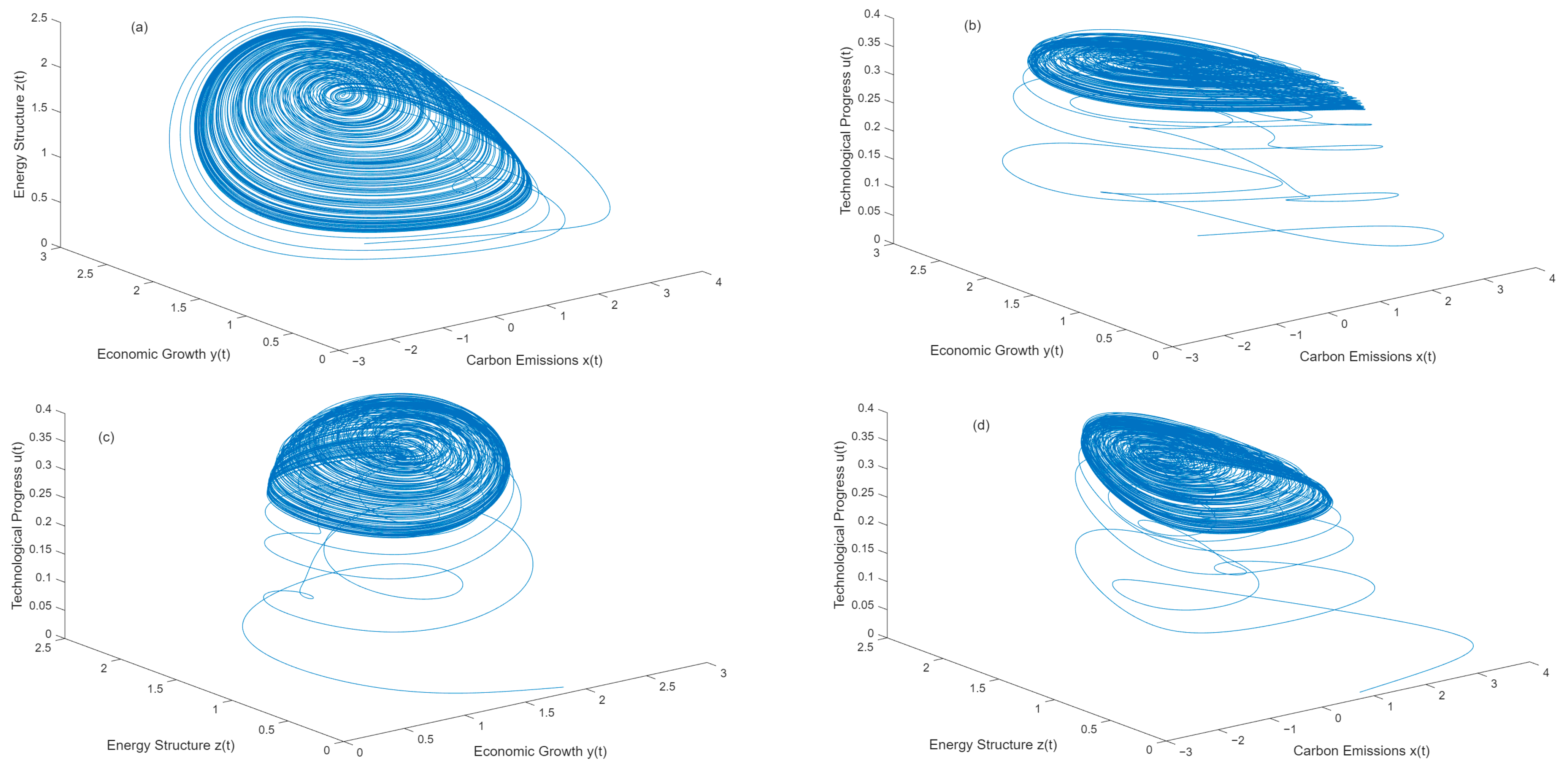
Case 1: Let the parameter a 2 = 0.8   in system (1), with the remaining parameters set to the values in Equation (2), and take the initial values as (0.758,1.83,0.015,0.01). At this time, the corresponding Lyapunov exponents are:  L 1 = 0.0735 , L 2 = 0.0105 , L 3 = 0.0670 , L 4 = 0.1142 . It is evident that system (1) has a positive maximum Lyapunov exponent. Therefore, the chaotic attractor of the dynamic system can be observed, as shown in Figure 1a–d.
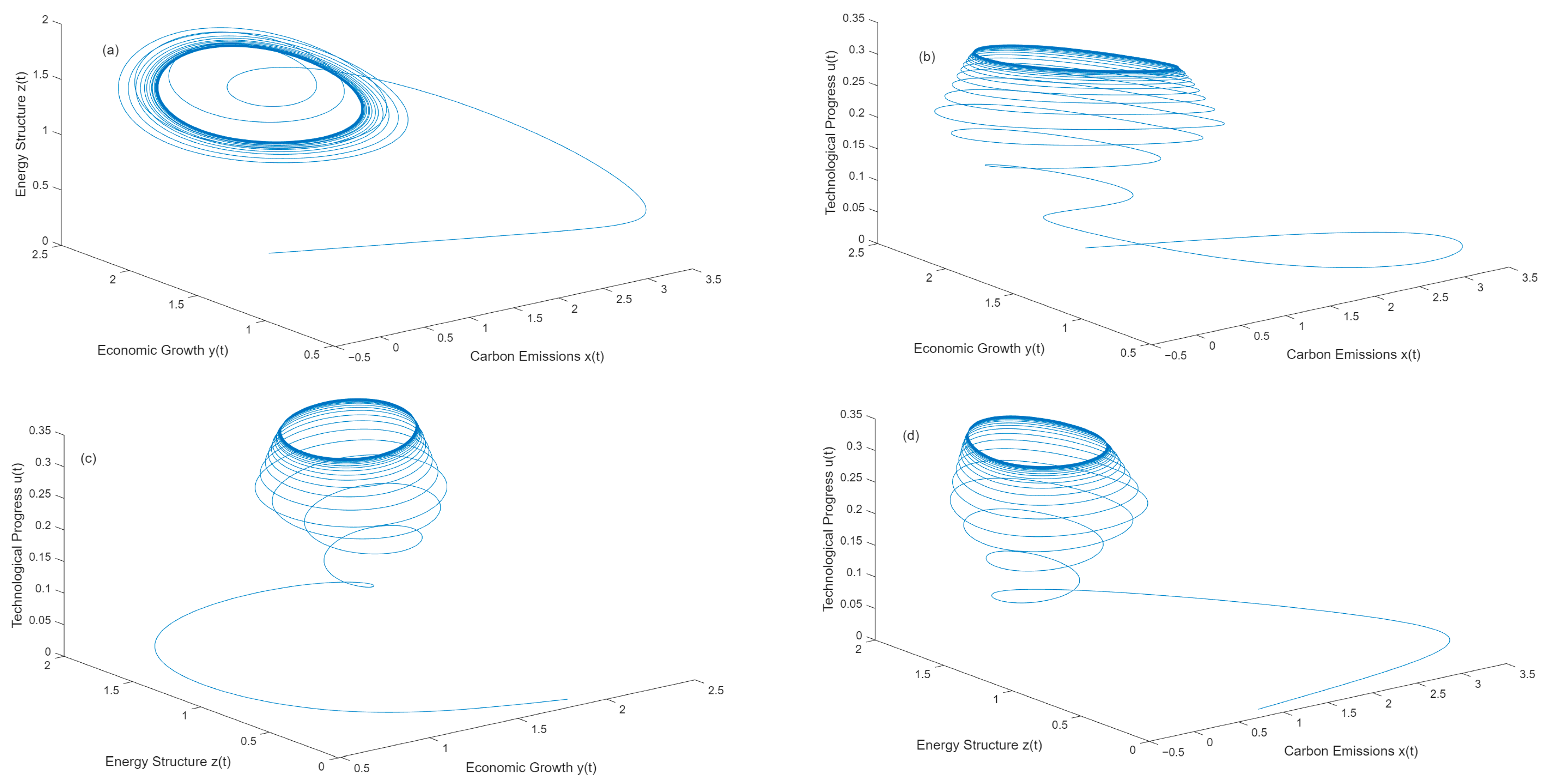
Case 2: Let the parameter a 2 = 0.7411   in system (1), with the remaining parameters set to the values in Equation (2), and take the initial values as (0.758,1.8,0.025,0.01). At this time, the corresponding Lyapunov exponents are L 1 = 0 , L 2 = 0.0219 , L 3 = 0.0291 , L 4 = 0.0675 . From the analysis, it is evident that the maximum Lyapunov exponent of system (1) is 0. Therefore, the limit cycle of the dynamic system can be observed, which is visually demonstrated in Figure 2a–d.
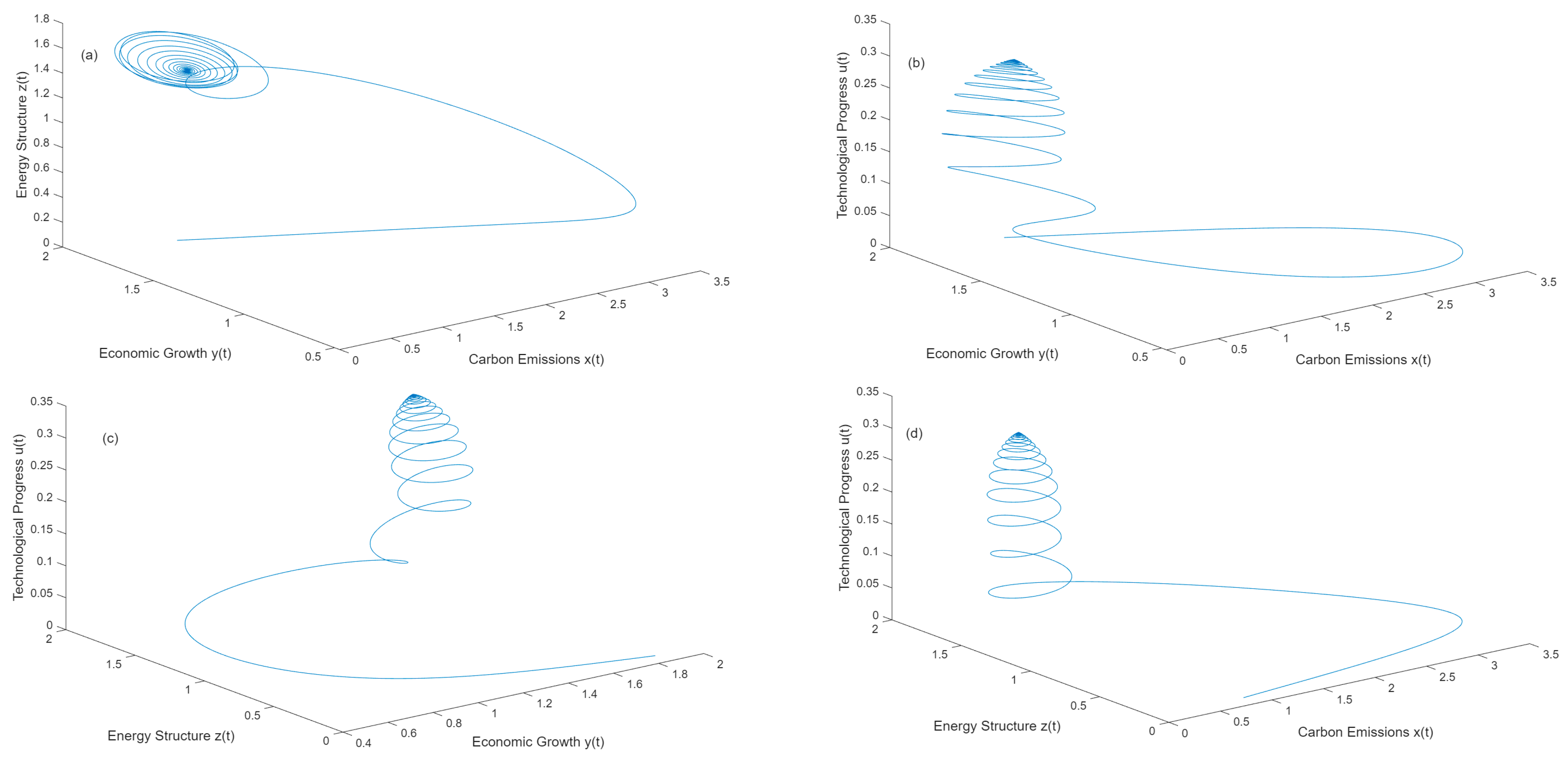
Case 3: Let the parameter a 2 = 0.71 in system (1), with the remaining parameters set to the values in Equation (2), and take the initial values as (0.758, 1.83, 0.025, 0.01). At this time, the corresponding Lyapunov exponents are L 1 = 0.0113 , L 2 = 0.0228 , L 3 = 0.0271 , L 4 = 0.0570 . The results indicate that the maximum Lyapunov exponent of system (1) is negative. Therefore, the stable equilibrium point of the dynamic system can be observed, as illustrated in Figure 3a–d.
The aforementioned numerical simulations demonstrate that the interrelationships between technological progress, carbon emissions, economic growth, and energy structure display highly complex nonlinear features. This complexity is closely associated with the parameters within the model, which assume distinct values across different periods and under varying contextual conditions. Different parameter values cause the system to present stable states (Figure 3), periodic states (Figure 2), and chaotic states (Figure 1). Meanwhile, the numerical simulation results also reveal that under the same parameter settings but different initial conditions, the system exhibits diverse chaotic behaviors, which indicates that the system is sensitive to initial conditions.
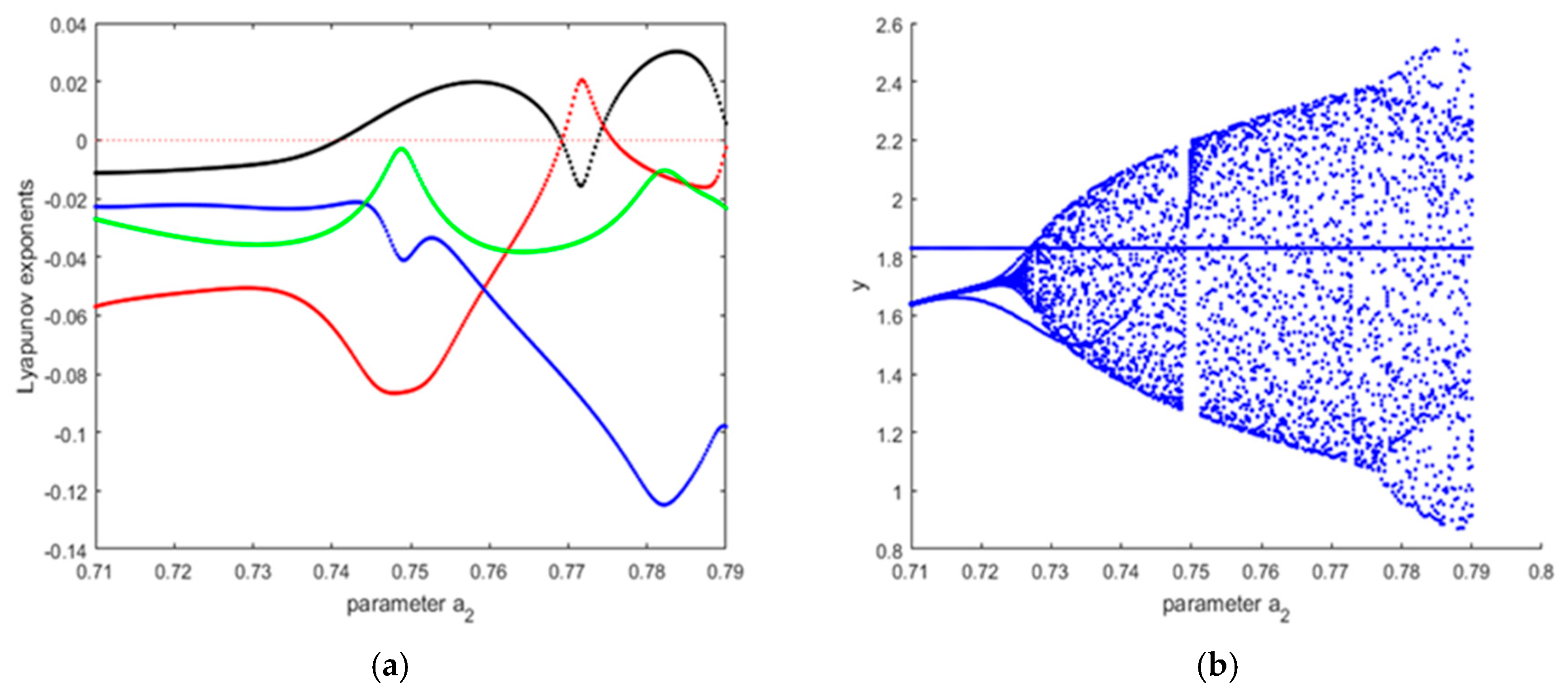
Letting the parameter a 2 vary while keeping other parameters fixed at the values in Case 1, we obtain the Lyapunov exponents of variable y with respect to parameter a 1 and the corresponding one-parameter bifurcation diagram, as shown in Figure 4a,b. The following conclusions can be drawn: when   a 2 0.71 ,   0.741 , the maximum Lyapunov exponent of system (1) is less than 0, indicating that the system has a stable equilibrium point (for example, when a 2 = 0.71 , the system trajectory is shown in Figure 3); when   a 2 = 0.7411 , the maximum Lyapunov exponent equals 0, indicating that the system has a periodic orbit (the system trajectory is shown in Figure 2); when a 2 0.741 ,   0.79 , system (1) has a positive Lyapunov exponent, indicating that system (1) is in a chaotic state (the system trajectory is shown in Figure 1). According to Figure 4b, the transition process of system (1) from periodic to chaotic as   a 2   increases can be clearly observed.
As revealed by the foregoing analysis, parameters exert a significant influence on the state of the system. Variations in parameter intervals will lead the system to exhibit distinct states. Thus, for a practical system, the state that the system will attain can be determined by identifying the parameter range. As shown in Figure 4a, when   a 2 0.741 ,   0.79 , the technological progress–carbon emissions–economic growth–energy structure system will exhibit a chaotic state, which is detrimental to economic and social development. In this case, certain measures need to be taken to reduce the value of the parameter   a 2 , thereby bringing the system to a stable state. If the means corresponding to effectively controlling the magnitude of the parameters can be identified based on the practical significance of the parameters, then the system can be used to conduct evolutionary analysis of the impacts of various regulatory measures on the system state.

2.3. Analysis of Dynamical Characteristics of the Subsystem

In this section, we analyze the dynamical characteristics of a subsystem derived from dynamic system (1), taking the carbon emissions–technological progress–energy structure subsystem as an example. Assuming steady economic development over a certain period and considering the coupling relationships among these three factors, we derive the following subsystem from system (1):
x ˙ = a 1 x 1 x C a 3 z a 4 u z ˙ = c 1 z x H 1 + c 3 u u ˙ = d 1 u x N
This subsystem reflects the interrelationships among carbon emissions, technological progress, and energy structure. This is a three-dimensional nonlinear system, and the Jacobian matrix of the system is
J = a 1 2 a 1 x / C a 3 a 4 c 1 z / H c 1 x H 1 c 3 d 1 u 0 d 1 x N
The calculation yields three non-zero equilibrium points: S 1 = x 1 , z 1 , u 1 , S 2 = x 2 , z 2 , u 2 , S 3 = x 3 , z 3 , u 3 , where x 1 = C , z 1   = 0 , u 1 = 0 ; x 2 = H , z 2 = a 1 H C H a 3 C , u 2 = 0 ; x 3 = N , z 3 = a 1 c 3 H N a 1 C N a 4 c 1 C H N + a 3 c 3 C H , u 3 = a 1 c 1 N N 2 C N H N + C H N a 4 c 1 C H N + a 3 c 3 C H .
(1) 
Stability of equilibrium point  S 1 = x 1 , z 1 , u 1
For the equilibrium point S 1 = x 1 , z 1 , u 1 , the coefficient matrix of the linearized system is
J 1 = a 1 a 3 a 4 0 c 1 C H 1 c 3 0 0 d 1 C N .
The eigenvalues of J 1 are λ 1 = d 1   C N , λ 2 = c 1   C / H 1 , λ 3 = a 1 . Thus, for the equilibrium point S 1 = x 1 , z 1 , u 1 , the following conclusions can be drawn:
(i)
When C < N and C H < 1 , the equilibrium point S 1 = x 1 , z 1 , u 1 is asymptotically stable. The practical significance of this case is that total carbon emissions stabilize at a constant value, and the carbon emissions at this time are within the range permitted by the environment, i.e., C < N and C H < 1 , indicating that it is no longer necessary to reduce carbon emissions through energy structure adjustment and technological innovation.
(ii)
When C > N or C H > 1 , the equilibrium point S 1 = x 1 , z 1 , u 1 is unstable. The practical significance of this case is that total carbon emissions exceed the maximum carrying capacity of the environment. At this time, external measures are needed, such as increasing research and development efforts in technological innovation and accelerating the optimization and adjustment of energy structure, to control carbon dioxide emissions and achieve sustainable development.
(2) 
Stability of equilibrium point  S 2 = x 2 , z 2 , u 2
For the equilibrium point S 2 = x 2 , z 2 , u 2 , the coefficient matrix of the linearized system is
J 2 = a 1 2 a 1 H C a 3 a 4 a 1 c 1 C H a 3 C 0 c 3 0 0 d 1 H N
The eigenvalues of J 2 are
λ 1 = d 1 H N , λ 2 , 3 = ( a 1 C 2 a 1 H ) ± 4 a 1 c 1 C 3 H C + a 1 C 2 a 1 H 2 2 C .
Thus, for the equilibrium point S 2 = x 2 , z 2 , u 2 , the following conclusions can be drawn:
(i)
If H < N and a 1 C < 2 a 1 H , the equilibrium point S 2 = x 2 , z 2 , u 2 is asymptotically stable. The practical significance of this case is that total carbon emissions stabilize within the range permitted by the environment, and at this time, it is not necessary to reduce carbon emissions through energy structure optimization and technological progress.
(ii)
If H > N , the equilibrium point S 2 = x 2 , z 2 , u 2 is unstable. The practical significance of this case is that, compared with energy structure adjustment, the increase in carbon emissions will prioritize the innovation and application of green technologies.
(iii)
If H > N and a 1 C > 2 a 1 H , then λ 2 , 3 are a pair of complex conjugate roots with positive real parts, and S 2 = x 2 , z 2 , u 2 is an unstable saddle point.
(iv)
If a 1 C = 2 a 1 H  and H < C , then λ 2 , 3 are a pair of purely imaginary conjugate roots, resulting in a Hopf bifurcation. This indicates that before and after the Hopf bifurcation, the system changes from stable to unstable. Therefore, the system can be brought to a stable state by adjusting the degree of energy structure optimization, thereby promoting sustainable economic and social development.
(3) 
Stability of equilibrium point  S 3 = x 3 , z 3 , u 3
For the equilibrium point S 3 = x 3 , z 3 , u 3 , the coefficient matrix of the linearized system is
J 3 = a 1 2 a 1 N / C a 3 a 4 c 1 a 1 c 3 N a 1 C N φ c 1 N H 1 c 3 d 1 a 1 c 1 N N 2 C N H N + C H N φ 0 0 .
where φ = a 4 c 1 C H N + a 3 c 3 C H . For simplicity, the coefficients are fixed as: a 1 = 0.088 , a 3 = 0.412 , a 4 = 0.072 , c 1 = 0.09 , c 3 = 0.096 , d 1 = 0.01 , C = 1.6 , H = 0.9 , N = 1.62 . At this time, the equilibrium point is S 3 = 1.62 , 0.381 , 0.239 , and the eigenvalues of J 3 are λ 1 = 0.1595 < 0 , λ 2 = 0.1375 > 0 , λ 3 = 0.0037 > 0 . Therefore, the equilibrium point S 3 is an unstable saddle point.
As demonstrated in the analysis, the stability of the subsystem composed of carbon emissions, technological progress and energy structure at equilibrium points S 1 , S 2 and S 3 hinges entirely on system parameters, showing both stable and unstable states. Hence, this three-dimensional system possesses sophisticated dynamic properties.
Similarly, in the dynamic system (1), if the change in energy structure is not considered, the coupling relationships among technological progress, carbon emissions, and economic growth can be studied. In system (1), setting z = 0 yields the technological progress–carbon emissions–economic growth subsystem:
x ˙ = a 1 x 1 x C + a 2 y 1 y E a 4 u y ˙ = b 1 x b 2 y + b 4 u u M 1 u ˙ = d 1 u x N + d 2 y .
Considering the coupling relationships among technological progress, economic growth, and energy structure under the condition that the total regional carbon emissions are fixed, setting x = K in system (1) yields the technological progress–economic growth–energy structure subsystem:
y ˙ = b 2 y + b 3 z z L 1 + b 4 u u M 1 z ˙ = c 1 z K 1 H 1 + c 2 y + c 3 u u ˙ = d 1 u K 2 N + d 2 y .
The dynamical characteristics of the above two subsystems can be analyzed by referring to the method for analyzing the dynamical characteristics of the carbon emissions–technological progress–energy structure subsystem.

3. Empirical Analysis

3.1. Parameter Identification

Carbon emission data are retrieved from the China Carbon Accounting Database (CEADS). Data on economic growth and energy structure are sourced from the China Statistical Yearbook, where economic growth is measured by GDP, and energy structure is measured by the share of primary electricity and other energy sources in total energy consumption. This study focuses on green innovation activities; accordingly, green technology patents of Chinese A-share listed firms are adopted to characterize technological progress. It is widely acknowledged that granted patents better reflect the actual quality and capacity of corporate green innovation, whereas patent applications merely indicate firms’ emphasis on green technology research. For this reason, this paper employs the number of granted green patents to quantify technological progress, with relevant data obtained from the China Research Data Service Platform. Taking 2009 as the base year, Table 1 presents the ratios of the relevant indicators from 2010 to 2019 relative to the 2009 baseline level.
Using the systematic variable ratio data from 2010 to 2019 as the original samples, the data set is divided into training and test sets at a ratio of 7:3 according to the characteristics of time-series data, where the data from 2010 to 2016 are used as the training set for parameter optimization, and the data from 2017 to 2019 are used as the test set for verifying the generalization ability of the model. The min-max normalization method is adopted to preprocess the input and output variables, and the normalization statistics are calculated only from the training set to avoid data leakage. The model parameters to be identified, namely a1, a2, a3, a4, b1, b2, b3, b4, c1, c2, c3, d1, d2, are encoded as individuals in the genetic algorithm population. The population size is set to 50, the maximum number of iterations to 1000, the crossover probability to 0.8, and the mutation probability to 0.01. The fitness function is constructed using the sum of squared errors between the model outputs and the actual values of the training set. Through iterative optimization involving selection, crossover, and mutation, the model parameter combination that minimizes the fitting error on the training set and achieves the optimal generalization error on the test set is finally output, completing the determination of the system model parameters. The pseudocode is shown in Table 2.
In this paper, there are 13 parameters to be identified, with a population size of 50 and a maximum number of iterations of 1000. The overall algorithm exhibits polynomial time complexity O(G × N × D), where G denotes the maximum number of iterations, N the population size, and D the number of parameters to be optimized. The parameter and iteration settings are moderate, which can ensure sufficient search space for global optimization without incurring excessive computational overhead. The crossover and mutation operations are local linear computations and do not introduce exponential complexity. Meanwhile, the fitness function only requires forward calculation of the four-dimensional dynamic system, resulting in light and controllable computational cost. Therefore, the overall computational complexity can be efficiently executed on conventional personal computers and numerical computing platforms, maintaining high computational efficiency while meeting the accuracy requirements of parameter identification. The calculated parameters of the actual system are shown in Table 3.
Taking the system parameters as those in Table 1 and taking the data from 1990 as the initial conditions, x t = 0.209 , with the unit being 10 10 tons; y t = 0.0018873 , with the unit being 10 15 yuan; z t = 0.15 , representing the proportion of primary power and other energy sources in total energy consumption in China in 1990; u t = 0.000001 . The number of green patents granted to Chinese A-share listed companies in 1990 was zero, which is taken as 1 × 10 6 for the convenience of study. Thus, the initial condition is [0.209, 0.0018873, 0.15, 0.000001]. Figure 5 presents the phase diagram of the actual system under these conditions. As observed from the phase trajectory, the system reaches a stable state, which is consistent with real-world practical situations.

3.2. Analysis of Regulatory Policies Based on Model Parameters

3.2.1. Regulatory Strategy 1: Adjusting the Intensity of Investment in Technology Research and Development

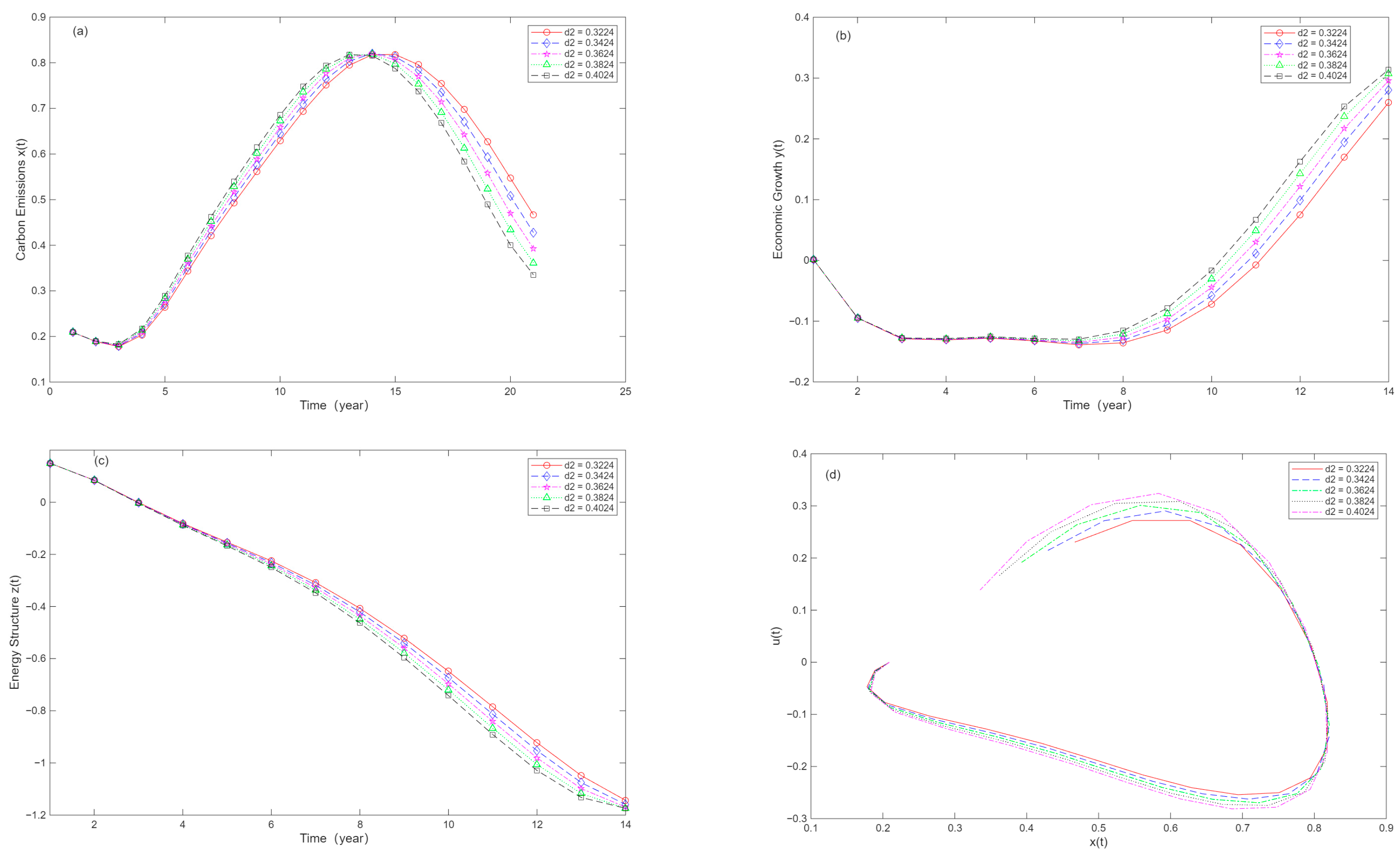
In this model, the parameter d 2 denotes the influence coefficient of economic growth on technological progress. Its variation reflects changes in technological innovation investment; specifically, a larger value of d 2 corresponds to greater attention and higher capital input devoted to innovation activities. With all system parameters fixed according to Table 3 and the initial condition set as [0.209, 0.0018873, 0.15, 0.000001], the value of d 2 is allowed to change. Figure 6a–d illustrate the evolutionary trends of carbon emissions, economic growth and energy structure, along with the phase diagram between technological progress and carbon emissions under the gradual increase in d 2 .
Figure 6a illustrates the positive impact of investment in technological innovation on carbon emissions. Comparing the five curves in the figure, it can be observed that when the model parameter d 2 gradually increases, the early evolution behavior of carbon emissions shows little difference, and the peak values are approximately equal. However, a larger d 2 enables carbon emissions to reach their peak earlier, and after the peak, the larger the value of d 2 , the faster the carbon emissions decline. This indicates that increasing investment in technological innovation can lead to an earlier peak in carbon emissions. When technological progress reaches a certain threshold, its emission reduction effect gradually emerges. With the continuous accumulation of technological advancements, the decline rate of carbon emissions is further accelerated. This trend is particularly pronounced when the value of d 2 is high.
Figure 6b illustrates how technological innovation investment influences economic growth. As the value of d 2 increases, i.e., as investment in technological innovation increases, it can be observed that the economic growth rate exhibits different trends in different time periods. Specifically, in the initial stage (within 8 years), the economic growth level is relatively low. This is the result of the combined effects of the lag effect of technological innovation, the investment return cycle, and the market adaptation period. That is, in the early stage, substantial R&D investment may not immediately yield significant economic returns, and the market acceptance of new technologies takes time, leading to a temporary decline in the economic growth rate. In the subsequent stage (8–14 years), as technological innovation accumulates, the economic growth rate gradually rises. At the same time, it can be observed that changes in the value of d 2 have a negligible impact on economic growth in the initial stage, but in the subsequent stage, the larger the value of d 2 , the faster the economic growth rate. This indicates that increasing investment in technological innovation may not immediately bring about significant economic growth in the short term, but its driving effect on economic growth will gradually become apparent in the medium and long term. This trend is particularly pronounced when the value of d 2 is high, i.e., when investment in technological innovation is large, the upward trend in economic growth in the medium and long term is more obvious.
Figure 6c depicts the influence of technological innovation investment on the evolution of energy structure. It can be observed that investment in technological innovation leads to a downward trend in the energy structure. This is due to the initial costs of energy structure transformation and the lag effect of technological innovation. As technological innovation advances, the proportion of traditional energy sources (such as coal and oil) gradually decreases, which may lead to temporary instability in energy supply or an increase in costs, thereby manifesting as negative growth in the short term. Clean energy technologies may take time to mature and be widely applied. Before these technologies are fully mature, their efficiency and economic benefits may be insufficient to compensate for the impact of the reduction in traditional energy. Although the energy structure exhibits a downward trend in the short term, in the long run, technological innovation and the promotion of clean energy will lead to a more sustainable energy supply and lower carbon emissions.
Figure 6d presents the phase diagram between technological progress and carbon emissions. It can be observed that variations in d 2 lead to distinct evolutionary relationships between the two variables. At the initial stage, technological progress grows slowly while carbon emissions remain at a relatively high level. As innovation accumulation deepens, the advancement of technology accelerates gradually; after reaching its peak, carbon emissions begin to decline noticeably. In the later stage, technological progress rises substantially, accompanied by a marked reduction in carbon emissions, which clearly demonstrates the inhibitory effect of technological innovation on carbon emissions. A comparison among the five curves further indicates that a larger d 2 corresponds to a faster upward trend in technological progress, reflecting a stronger accumulation effect of innovation investment. Meanwhile, higher values of d 2 bring about a more prominent decline in carbon abatement. This finding verifies the positive role of technological innovation in emission reduction. Overall, increasing investment in technological innovation can accelerate technological upgrading and curb carbon emissions in the long run, thereby effectively promoting sustainable development.

3.2.2. Regulatory Strategy 2: Adjusting the Level of Energy Structure Optimization

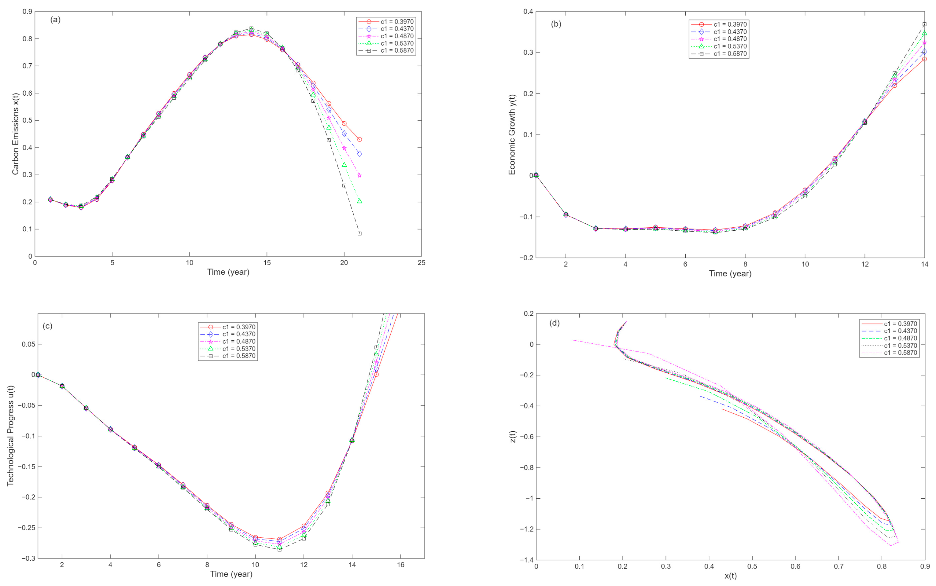
The parameter c 1 in the model is the development coefficient of energy structure, and the variation in c 1 reflects the development level of the energy structure itself. A larger value of c 1 indicates a more optimized energy structure, meaning that more clean energy (such as wind power, solar energy, etc.) is introduced into the energy system, thereby reducing dependence on fossil fuels. Fixing the system parameters as those in Table 3, with the initial condition [0.209,0.0019,0.15,0.000001], the simulation yields the evolution paths of carbon emissions, economic development, and technological progress, as well as the phase diagram of energy structure and carbon emissions under variations in c 1 , as shown in Figure 7a–d.
Figure 7a shows the trends in carbon emissions under different levels of energy structure optimization. It can be seen that when c 1 gradually increases, the early evolution behavior of carbon emissions shows essentially no difference, indicating that relying solely on the development of the energy structure itself cannot effectively reduce carbon emissions in the initial stage. In the medium term, a larger value of c 1 corresponds to a higher peak in carbon emissions. In the later stage, as the value of c 1 increases (e.g., c 1 = 0.5870 ), the energy structure optimization reaches a certain level, carbon emissions decrease significantly, and the rate of decline accelerates, indicating that in the long run, rapid optimization of the energy structure can reduce carbon emissions more effectively. These scenarios suggest that energy structure optimization is a complex process, and a balance between the short term and the long term needs to be found to achieve sustainable emission reduction goals.
Figure 7b shows the evolution of economic growth when the value of c 1 varies. It can be observed that economic growth exhibits a trend of first declining, then stabilizing, and then increasing significantly. In the initial stage (0–5 years), the initial transformation of the energy structure may lead to a temporary decline in economic growth, as new energy infrastructure requires investment and time to construct. In the medium term (5–9 years), as clean energy is gradually introduced and the energy structure is optimized, economic growth begins to show a positive trend. In the long term (9–14 years), the energy structure is fully optimized, significantly reducing dependence on fossil fuels and mitigating the impact of energy price fluctuations on the economy, resulting in rapid, more stable, and sustainable economic growth. In addition, in the initial and medium-term stages, different values of c 1 do not cause significant changes in economic growth, but in the long term, as the value of c 1 increases, the economic growth rate improves. This indicates that in the long run, a higher level of energy structure optimization can promote sustainable economic development, thereby contributing to long-term economic prosperity.
Figure 7c shows the trend of technological progress over time. In the early stage (0–11 years), technological progress in clean energy exhibits a downward trend, primarily due to the lag effect of technology research and development, the investment pressure and resource reallocation during the initial phase of energy structure transformation, the exit costs of traditional technologies, and the time gap in the diffusion and application of new technologies. In the later stage (11–16 years), as clean energy technologies mature and are widely applied, technological progress continues to accelerate, bringing significant long-term economic and environmental benefits. The evolutionary trends of technological progress under different values of c 1 differ slightly. A higher value of c 1 corresponds to a lower level of technological progress, which is because a higher c 1 value implies a more rapid optimization of the energy structure, requiring more extensive technology substitution and infrastructure renewal, leading to greater technological challenges in the short term. However, in the long term, a higher value of c 1 leads to more significant technological progress.
Figure 7d shows the phase diagram of energy structure and carbon emissions under variations in c 1 . It can be observed that the energy structure exhibits a trend of first declining and then rising, while carbon emissions show a trend of first increasing and then decreasing. The optimization of energy structure is negatively correlated with carbon emissions, which is consistent with the previous analysis. The impacts of different values of c 1 on energy structure and carbon emissions are reflected in the later stage: a low value of c 1 (e.g., c 1 = 0.3970 ,   0.4370 ) indicates a relatively high proportion of fossil fuels in the energy structure and higher carbon emissions; at this stage, the optimization of the energy structure has a limited effect on reducing carbon emissions. A medium value of c 1 (e.g., c 1 = 0.4870 ,   0.5370 ) corresponds to an increased share of clean energy and a significant decline in carbon emissions, representing a critical period in the transformation of the energy structure. A high value of c 1 (e.g., c 1 = 0.5870 ) indicates that clean energy dominates the energy structure, with carbon emissions further decreasing and potentially approaching near-zero emission levels. This demonstrates that promoting the development of clean energy and improving the level of energy structure optimization have significant long-term effects on reducing carbon emissions.

3.2.3. Regulatory Strategy 3: Analysis of Carbon Emissions and Economic Development Under Combined Strategies

Comparing Figure 6a and Figure 7a, it can be observed that carbon emissions in the former reach their peak slightly earlier, while in the latter, carbon emissions decline more rapidly after reaching the peak. This indicates that in terms of reducing carbon emissions, increasing investment in technological progress is more effective than relying on the development of the energy structure itself, and is thus a key factor in controlling carbon emissions. Comparing Figure 6b and Figure 7b, it can be observed that increasing the value of d 2 can promote economic growth earlier and more rapidly, while a larger value of c 1 corresponds to a higher economic growth rate. This indicates that increasing investment in technological progress can effectively promote economic growth in the medium term, while relying on the development of the energy structure itself can drive the economy to a higher stage in the long term.
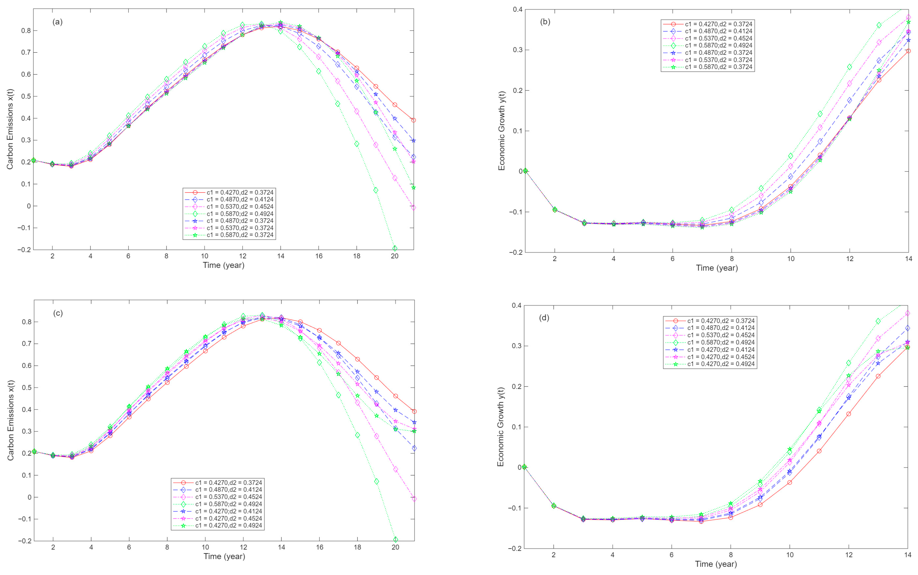
Based on the parameters in Table 3, comparing the adjustment of a single parameter c 1 or d 2 with the simultaneous adjustment of both c 1 and d 2 , i.e., comparing the evolution trends of carbon emissions and economic development under single-policy adjustments and combined policy adjustments, the following results are obtained. The evolution of carbon emissions over time (Figure 8a) and the evolution of economic development over time (Figure 8b) are shown for the combined policy of increasing investment in technological innovation (increasing the value of the parameter d 2 ) and optimizing energy structure (increasing the value of the parameter c 1 ) versus the single policy of only optimizing energy structure. The evolution of carbon emissions over time (Figure 8c) and the evolution of economic development over time (Figure 8d) are shown for the combined policy versus the single policy of only increasing investment in technological innovation.
Overall, the evolutionary trends of carbon emissions and economic development under combined policies and single policy interventions are generally consistent: carbon emissions all present an inverted U-shaped pattern of rising first and then falling, with roughly similar peak levels; economic growth follows an evolutionary pattern of initial decline, followed by stabilization, and subsequent rapid growth.
As illustrated in Figure 8a,c, both single policies and combined policies lead to a slight increase in carbon emissions in the initial implementation stage, while the incremental carbon emissions induced by single policies are marginally higher than those under combined policies. The baseline scenario is set as c 1 = 0.4270 and d 2 = 0.3724 . Under the combined policy scenario ( c 1 = 0.4870 , d 2 = 0.4124 ), carbon emissions peak in the 13th year, with an average emission reduction rate of 5.597% in the five years after the peak. Under the single energy structure adjustment scenario ( c 1 = 0.4870 , d 2 = 0.3724 ), carbon emissions reach their peak in the 14th year, with an average emission reduction rate of 1.758% in the five post-peak years. Under the single low-carbon technology development scenario ( c 1 = 0.4270 , d 2 = 0.4124 ), carbon emissions also peak in the 14th year, with an average emission reduction rate of 4.631% over the subsequent five years.
It can be observed from Figure 8b,d that single policies and combined policies show no significant difference in their impact on economic growth in the early implementation stage. In the later stage, the driving effect of combined policies on economic growth is remarkably stronger than that of the single energy structure adjustment policy. Taking c 1 = 0.4270 and d 2 = 0.3724 as the baseline scenario: Under the combined policy scenario ( c 1 = 0.4870 , d 2 = 0.4124 ), the combined policy significantly boosts economic growth starting from the 11th year, with an average growth enhancement of 15.877% over five years. Under the single energy structure adjustment scenario ( c 1 = 0.4870 , d 2 = 0.3724 ), the policy also promotes economic growth from the 11th year onward, achieving an average improvement of 8.827% within five years. Under the single low-carbon technology development scenario ( c 1 = 0.4270 , d 2 = 0.4124 ), the policy likewise drives economic growth beginning in the 11th year, with an average growth increase of 5.516% over the five-year period.

4. Discussion and Conclusions

Based on the nonlinear dynamics theory, this paper constructs a four-dimensional coupled dynamic system including technological progress, carbon emissions, economic growth and energy structure. Through theoretical analysis, numerical simulation and empirical parameter identification, this paper systematically reveals the internal laws of multi-factor collaborative evolution and the effects of policy regulation. The results show that the constructed system can effectively describe the nonlinear interaction mechanism of the energy–economy–environment–technology system. The change in parameters can drive the system to transition among stable state, periodic state and chaotic state. Among them, the key parameter a 2 (the driving coefficient of economic growth on carbon emissions) is the core threshold that determines the dynamic behavior of the system. When a2 falls within the interval [0.741, 0.79], the system enters a chaotic state, indicating that an excessively high intensity of economic-driven emissions will lead to system instability, so it is necessary to maintain the parameter within a stable range through regulation. The empirical results show that China’s actual system from 2010 to 2019 is in a stable equilibrium state, which is consistent with the macro-development reality.
The regulation and simulation results indicate that both single policy and combined policy can realize the coordination between carbon peaking and economic growth, but their effects are significantly different. Increasing investment in technological innovation (raising d 2 ) can advance the carbon peaking time, accelerate the decline after peaking, and exert a significant pulling effect on the economy in the medium term. Optimizing energy structure (raising c 1 ) plays a stronger role in long-term carbon emission reduction and economic growth. The combined policy (synergistically raising c 1 and d 2 ) is superior to single policies, with higher carbon emission reduction amplitude and more significant economic promotion effect, achieving a win–win situation of carbon reduction and growth. This suggests that low-carbon transformation should adhere to the coordination of technological innovation and energy structure upgrading, rather than relying on a single type of policy tool.
The subsystem analysis further shows that subsystems such as carbon emissions–technological progress–energy structure have multiple equilibrium points, whose stability is determined by parameter intervals. Some equilibrium points undergo Hopf bifurcation with parameter changes, indicating that appropriate regulation can guide the system to a stable path. Overall, the model in this paper can capture critical mutations, phased effects and initial value sensitivity of complex systems, providing a theoretical basis and quantitative reference for dynamic regulation under the dual-carbon goals.
The four-dimensional dynamic system constructed in this paper can effectively characterize the nonlinear evolution of technological progress, carbon emissions, economic growth and energy structure, but it still has certain limitations. The model only selects core variables and does not consider realistic factors such as energy costs, crisis shocks, regional heterogeneity and policy time lags, resulting in a relatively simplified system structure. Meanwhile, the deterministic framework is adopted without introducing random disturbances and multi-agent game behavior, so the fitting ability to complex reality needs to be improved. In the future, improvements can be made in many aspects: further expanding the variable dimension by integrating energy prices, industrial structure, regional differences and other factors; introducing random disturbances and time-varying parameters to construct a more realistic stochastic dynamic system; combining complex network and evolutionary game theory to depict the interactive behavior of government and enterprises; adopting hybrid intelligent algorithms to optimize parameter identification and carry out multi-policy collaborative scenario simulation, so as to enhance the model’s practical interpretability, prediction accuracy and policy reference value.


Author Contributions

Conceptualization, X.W. and H.X.; methodology, X.W. and Y.S.; software, X.W., H.X. and Z.S.; validation, X.W., H.X. and M.W.; writing—original draft preparation, X.W. and Y.S.; writing—review and editing, X.W. and H.X.; funding acquisition, H.X. and M.W. All authors have read and agreed to the published version of the manuscript.

Funding

This work was supported by the Major Project of the National Social Science Fund of China (22&ZD136), the major project of philosophy and social science research in colleges and universities of Jiangsu Province (2024SJZD129), the major project of Basic Science (Natural science) research in colleges and universities of Jiangsu Province (24KJA110002).

Data Availability Statement

Data will be made available on request.

Conflicts of Interest

The authors declare no conflicts of interest.

References

  1. Wang, J.; Xu, H.; Wang, M. Technology diffusion considering technological progress and multiple policy combinations based on evolutionary game theory. Technol. Soc. 2025, 81, 102799. [Google Scholar] [CrossRef] [Scilit]
  2. Guseo, R.; Guidolin, M. Cellular automata with network incubation in information technology diffusion. Phys. A Stat. Mech. Its Appl. 2010, 389, 2422–2433. [Google Scholar] [CrossRef] [Scilit]
  3. Reddy, B.S. Economic dynamics and technology diffusion in Indian power sector. Energy Policy 2018, 120, 425–435. [Google Scholar] [CrossRef] [Scilit]
  4. An, K.; Wang, C.; Cai, W. Low-carbon technology diffusion and economic growth of China: An evolutionary general equilibrium framework. Struct. Change Econ. Dyn. 2023, 65, 253–263. [Google Scholar] [CrossRef] [Scilit]
  5. Tsai, J.M.; Hung, S.W. A novel model of technology diffusion: System dynamics perspective for cloud computing. J. Eng. Technol. Manag. 2014, 33, 47–62. [Google Scholar] [CrossRef] [Scilit]
  6. Song, Y.; Lee, S.; Zo, H.; Lee, H. A hybrid Bass–Markov model for the diffusion of a dual-type device-based telecommunication service: The case of WiBro service in Korea. Comput. Ind. Eng. 2015, 79, 85–94. [Google Scholar] [CrossRef] [Scilit]
  7. Han, Z.; Tang, Z.; He, B. Improved Bass model for predicting the popularity of product information posted on microblogs. Technol. Forecast. Soc. Chang. 2022, 176, 121458. [Google Scholar] [CrossRef] [Scilit]
  8. Qiao, T.; Shan, W.; Zhang, M.; Liu, C. How to facilitate knowledge diffusion in complex networks: The roles of network structure, knowledge role distribution and selection rule. Int. J. Inf. Manag. 2019, 47, 152–167. [Google Scholar] [CrossRef] [Scilit]
  9. Losacker, S. License to green: Regional patent licensing networks and green technology diffusion in China. Technol. Forecast. Soc. Chang. 2022, 175, 121336. [Google Scholar] [CrossRef] [Scilit]
  10. Skoczkowski, T.; Bielecki, S.; Wojtyńska, J. Long-term projection of renewable energy technology diffusion. Energies 2019, 12, 4261. [Google Scholar] [CrossRef] [Scilit]
  11. Grabisch, M.; Rusinowska, A.; Venel, X. Diffusion in large networks. J. Econ. Dyn. Control. 2022, 139, 104439. [Google Scholar] [CrossRef] [Scilit]
  12. Wang, L.; Zheng, J. Research on low-carbon diffusion considering the game among enterprises in the complex network context. J. Clean. Prod. 2019, 210, 1–11. [Google Scholar] [CrossRef] [Scilit]
  13. Shi, Y.; Wei, Z.; Shahbaz, M.; Zeng, Y. Exploring the dynamics of low-carbon technology diffusion among enterprises: An evolutionary game model on a two-level heterogeneous social network. Energy Econ. 2021, 101, 105399. [Google Scholar] [CrossRef] [Scilit]
  14. Wu, Y.; Wang, X.; Liu, Z.; Zhao, X. Research on low-carbon technology diffusion among enterprises in networked evolutionary game. Chaos Solitons Fractals 2023, 174, 113852. [Google Scholar] [CrossRef] [Scilit]
  15. Shi, Y.; Han, B.; Zeng, Y. Simulating policy interventions in the interfirm diffusion of low-carbon technologies: An agent-based evolutionary game model. J. Clean. Prod. 2020, 250, 119449. [Google Scholar] [CrossRef] [Scilit]
  16. Fan, R.; Chen, R.; Wang, Y.; Wang, D.; Chen, F. Simulating the impact of demand-side policies on low-carbon technology diffusion: A demand-supply coevolutionary model. J. Clean. Prod. 2022, 351, 131561. [Google Scholar] [CrossRef] [Scilit]
  17. Ostovar, A.; Hajj, E.; Mehdizadeh, G.; Hand, A. Environmental Analysis of Emulsified Asphalt Products in the United States: A Comparative Cradle-to-Gate Life Cycle Assessment. Sustainability 2026, 18, 1821. [Google Scholar] [CrossRef] [Scilit]
  18. Pazouki, S.; Jamshidi, M.B.; Jalali, M.; Tafreshi, A. Transformative impact of AI and digital technologies on the FinTech industry: A comprehensive review. Int. J. Adv. Res. Humanit. Law 2025, 2, 1–27. [Google Scholar] [CrossRef] [Scilit]
  19. May, R.M. Simple mathematical models with very complicated dynamics. Nature 1976, 261, 459–467. [Google Scholar] [CrossRef] [Scilit]
  20. Farmer, J.D. Chaotic attractors of an infinite-dimensional dynamical system. Phys. D Nonlinear Phenom. 1982, 4, 366–393. [Google Scholar] [CrossRef] [Scilit]
  21. Farman, M.; Johansyah, M.D.; Raza, N.; Naik, M.K.; Sambas, A.; Nisar, K.S. Exploring Monetary Systems Through a Three-Dimensional Chaotic Framework with Fractional and Lyapunov Exponent Approach. Comput. Econ. 2026, 1–39. [Google Scholar] [CrossRef] [Scilit]
  22. Tarasyev, A.M.; Watanabe, C. Optimal dynamics of innovation in models of economic growth. J. Optim. Theory Appl. 2001, 108, 175–203. [Google Scholar] [CrossRef] [Scilit]
  23. Han, D.; Wang, R.; Yuan, Y.; Xiao, D. Research on the impact of ultra-high voltage transmission on urban carbon neutral technology innovation: An empirical test based on double machine learning method. Energy Econ. 2025, 154, 109120. [Google Scholar] [CrossRef] [Scilit]
  24. Fan, X.H.; Zhang, Y.; Yin, J.L. Evolutionary analysis of a three-dimensional carbon price dynamic system. Sustainability 2018, 11, 116. [Google Scholar] [CrossRef] [Scilit]
  25. Sun, M.; Tian, L.; Fu, Y. An energy resources demand-supply system and its dynamical analysis. Chaos Solitons Fractals 2007, 32, 168–180. [Google Scholar] [CrossRef] [Scilit]
  26. Sun, M.; Wang, X.; Chen, Y.; Tian, L. Energy resources demand-supply system analysis and empirical research based on non-linear approach. Energy 2011, 36, 5460–5465. [Google Scholar] [CrossRef] [Scilit]
  27. Tian, L.; Jin, R. Theoretical exploration of carbon emissions dynamic evolutionary system and evolutionary scenario analysis. Energy 2012, 40, 376–386. [Google Scholar] [CrossRef] [Scilit]
  28. Fang, G.; Tian, L.; Sun, M.; Fu, M. Analysis and application of a novel three-dimensional energy-saving and emission-reduction dynamic evolution system. Energy 2012, 40, 291–299. [Google Scholar] [CrossRef] [Scilit]
  29. Fang, G.; Tian, L.; Fu, M.; Sun, M. Government control or low carbon lifestyle: Analysis and application of a novel selective-constrained energy-saving and emission-reduction dynamic evolution system. Energy Policy 2014, 68, 495–507. [Google Scholar] [CrossRef] [Scilit]
  30. Wang, M.; Xu, H. A novel four-dimensional energy-saving and emission-reduction system and its linear feedback control. J. Appl. Math. 2012, 2012, 842716. [Google Scholar] [CrossRef] [Scilit]
  31. Wang, M.; Tian, L. Regulating effect of the energy market: Theoretical and empirical analysis based on a novel energy prices-energy supply-economic growth dynamic system. Appl. Energy 2015, 155, 526–546. [Google Scholar] [CrossRef] [Scilit]
Figure 1. Chaotic attractor of the dynamic system of technological progress, carbon emissions, economic growth, and energy structure, (a) x-y-z; (b) x-y-u; (c) y-z-u; (d) x-z-u.
Mathematics 14 01575 g001
Figure 2. Limit cycle of the dynamic system of technological progress, carbon emissions, economic growth, and energy structure, (a) x-y-z; (b) x-y-u; (c) y-z-u; (d) x-z-u.
Mathematics 14 01575 g002
Figure 3. Stable equilibrium point of the dynamic system of technological progress, carbon emissions, economic growth, and energy structure, (a) x-y-z; (b) x-y-u; (c) y-z-u; (d) x-z-u.
Mathematics 14 01575 g003
Figure 4. (a) Lyapunov exponent diagram and (b) bifurcation diagram of variable y .
Mathematics 14 01575 g004
Figure 5. Phase trajectory of the actual system.
Mathematics 14 01575 g005
Figure 6. The impact of changes in R&D investment intensity on system states: (a) impact of d 2 variation on carbon emissions, (b) impact of d 2 variation on economic development, (c) impact of d 2 variation on energy structure, (d) phase diagram of technological progress and carbon emissions under d 2 variation.
Mathematics 14 01575 g006
Figure 7. The impact of energy structure changes on system states: (a) impact of c 1 variation on carbon emissions, (b) impact of c 1 variation on economic development, (c) impact of c 1 variation on technological progress, (d) phase diagram of energy structure and carbon emissions under c 1 variation.
Mathematics 14 01575 g007
Figure 8. Evolution of system states under combined strategy regulation: (a) impact of the combined c 1 + d 2 policy and the single c 1 policy adjustment on carbon emissions, (b) impact of the combined c 1 + d 2 policy and the single c 1 policy adjustment on economic development, (c) impact of the combined c 1 + d 2 policy and the single d 2 policy adjustment on carbon emissions, (d) impact of the combined c 1 + d 2 policy and the single d 2 policy adjustment on economic development.
Mathematics 14 01575 g008
Table 1. Data for all system variables (2010–2019; 2009 as the base year).
Year x y z u Year x y z u
20101.07781.18251.10591.744920151.26181.97651.41186.1947
20111.19201.40000.98822.819520161.26222.14161.52947.2276
20121.23821.54531.14123.335220171.28292.38741.60009.1262
20131.30011.70141.20004.448220181.31192.63771.705912.2019
20141.28871.84661.32944.972020191.33562.83061.80009.0916
Table 2. Pseudocode of Parameter Identification by Genetic Algorithm.
% Data preparation
DATA = load(x, y, z, u, 2010–2019);
[TRAIN,TEST] = split(DATA,0.7);
[TRAIN_n,TEST_n] = normalize(TRAIN,TEST);
% GA initialization
Params = [a1, a2, a3, a4, b1, b2, b3, b4, c1, c2, c3, d1, d2];
PopSize = 50; MaxIter = 100;
Pc = 0.8; Pm = 0.01;
Pop = init(PopSize, Params);
% Fitness function
function f = fitness(ind)
[x_,y_,z_,u_] = model(ind);
err = sum((x_−x)2 + (y_−y)2 + (z_−z)2 + (u_−u)2);
f = 1/(1 + err);
end
% GA iteration
for iter = 1:MaxIter
Fit = fitness(Pop);
Pop = selection(Pop,Fit);
Pop = crossover(Pop,Pc);
Pop = mutation(Pop,Pm);
end
% Output
BestParam = best(Pop);
TestErr = evaluate(BestParam,TEST_n);
print(BestParam,TestErr);
Table 3. Parameter values of the actual system.
a 1 a 2 a 3 a 4 b 1 b 2 b 3 b 4 c 1 c 2
0.49160.38580.35680.44810.52480.51070.20180.28320.4270.5054
c 3 d 1 d 2 C E L M H N
0.43410.41080.37240.35330.63020.75520.45960.64780.6608
Disclaimer/Publisher’s Note: The statements, opinions and data contained in all publications are solely those of the individual author(s) and contributor(s) and not of MDPI and/or the editor(s). MDPI and/or the editor(s) disclaim responsibility for any injury to people or property resulting from any ideas, methods, instructions or products referred to in the content.