Complex Dynamics of a Supply–Demand–Price Network Model Incorporating a Marginal Feedback Mechanism

Abstract

In this paper, a supply–demand–price network model incorporating a marginal feedback mechanism is proposed to characterize the evolution of market prices. Unlike classical supply–demand models, the marginal effect of excess demand, defined as the rate of change in excess demand, is explicitly introduced into the price adjustment process. As the coefficient of the marginal feedback term varies, the system exhibits rich and complex nonlinear dynamics. In particular, the model gives rise to a centrally symmetric double-wing chaotic attractor, as well as a pair of coexisting single-wing chaotic attractors. The transition routes among different dynamical regimes are systematically analyzed using phase portraits, bifurcation diagrams, and Lyapunov exponents. Furthermore, multistability phenomena are observed, including the coexistence of equilibrium points, limit cycles, and chaotic attractors. The corresponding basins of attraction are illustrated to reveal their intricate and interwoven structures. In addition, the emergence of endogenous chaos is investigated through both theoretical analysis and numerical simulations. Finally, the consistency between the model dynamics and real market data provides empirical evidence supporting the validity and applicability of the proposed framework.

1. Introduction

Market mechanisms play a fundamental role in optimizing resource allocation, where price adjustment is primarily driven by the imbalance between supply and demand. The evolution of market prices has been extensively studied through various mathematical and economic models [1,2,3,4,5,6,7,8]. In classical microeconomics, Marshall’s equilibrium price theory states that prices rise when demand exceeds supply and fall when supply exceeds demand, eventually converging to an equilibrium state [9]. This framework has long served as a cornerstone for understanding price formation and market dynamics.

However, empirical evidence suggests that price evolution in real markets often deviates from this idealized mechanism [10]. In practice, individuals exhibit bounded rationality, and their decisions are influenced not only by market fundamentals but also by behavioral factors such as psychological panic [11,12] and memory effects [13]. As a result, expectations—whether optimistic or pessimistic—can significantly shape market dynamics. In particular, rapid changes in excess demand may trigger panic responses, leading to collective behavioral reactions that amplify market fluctuations. Such clustering effects may further destabilize the system and even induce abrupt transitions in market states. Existing studies on price dynamics mainly include econophysics models, adaptive expectation models, and higher-order dynamical systems. Econophysics models focus on statistical properties of price fluctuations, while adaptive expectation models emphasize behavioral feedback mechanisms. Meanwhile, higher-order systems such as jerk and hyper-jerk systems introduce derivative feedback to generate complex dynamics. However, the integration of marginal feedback of excess demand into a supply–demand–price framework remains largely unexplored.

Motivated by these observations, this paper develops a supply–demand–price dynamical model in which the marginal effect of excess demand, i.e., the rate of change in excess demand, is incorporated into the price adjustment mechanism. Under this formulation, price evolution depends not only on the magnitude of supply–demand imbalance but also on its rate of change. The resulting nonlinear system exhibits rich dynamical behaviors, including multistability, complex basin structures, and path-dependent outcomes [14,15,16]. Furthermore, inspired by higher-order derivative dynamical systems such as jerk and hyper-jerk systems [15,17,18], we investigate the emergence of so-called endogenous chaos generated by different derivative orders. The results demonstrate that the system can produce coexisting point attractors, periodic attractors, and chaotic attractors, revealing intricate dynamical mechanisms underlying market price evolution. Compared with classical supply–demand models, which typically consider only the level of excess demand, the proposed model incorporates the marginal feedback of excess demand into the dynamical process. Unlike adaptive expectation models and higher-order systems where derivative terms are often introduced from a purely mathematical perspective, the present framework provides a clear economic interpretation of such feedback within a unified supply–demand–price structure. Consequently, the model captures richer dynamical phenomena, including multistability, coexisting attractors, and endogenous chaos, which are rarely addressed in classical models. The main contributions of this paper are summarized as follows: (1) a supply–demand–price dynamical model incorporating marginal feedback is proposed, extending classical economic adjustment mechanisms; (2) the model reveals complex nonlinear behaviors, including multistability and coexisting attractors induced by derivative feedback; (3) a dynamical interpretation of endogenous chaos generated by higher-order derivative systems is provided; (4) the model is validated using real-world oil market data.

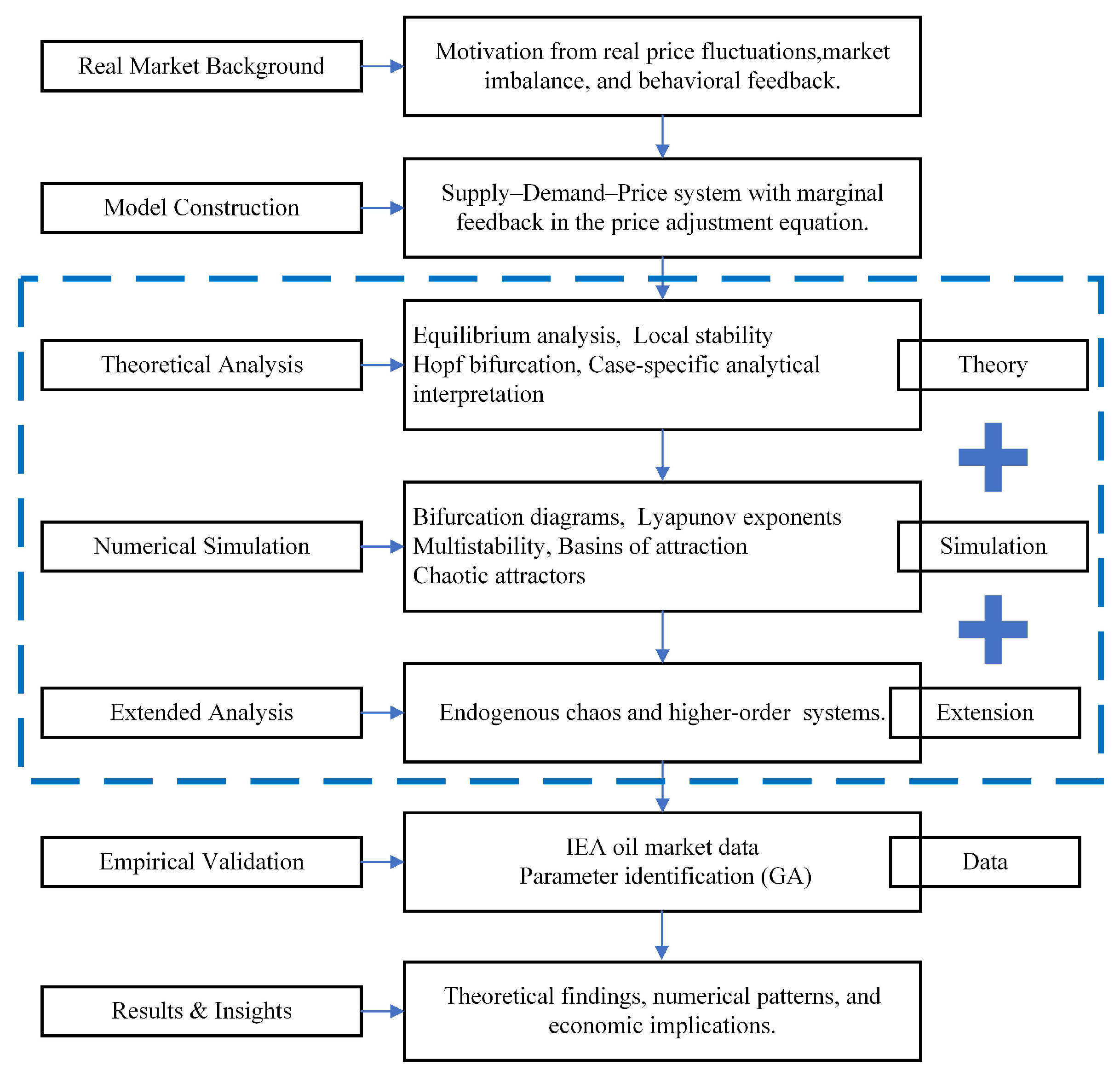
The overall research framework of this paper is illustrated in Figure 1. The remainder of the paper is organized as follows. Section 2 formulates the model. Section 3 analyzes local stability and Hopf bifurcation. Section 4 investigates global dynamics, including multistability and chaotic attractors. Section 5 presents parameter identification and empirical validation. Finally, Section 6 concludes the paper.

2. Model

In classical microeconomics, price adjustment is mainly driven by the imbalance between supply and demand. According to Marshall’s equilibrium theory, the rate of price change depends on the excess demand in the market. This relationship can be expressed as

$${\displaystyle \frac{dP}{dt}}=f(q)=f(D-S),$$

(1)

where P denotes the market price of the commodity, D and S represent demand and supply, respectively, and $q=D-S$ denotes the excess demand. The function $f(x)$ is usually assumed to satisfy $x f(x)\ge 0$, meaning that the price increases when demand exceeds supply and decreases when supply exceeds demand. In many studies, $f(x)$ is further assumed to be monotonically increasing [19,20,21,22].

However, in real markets, price adjustments may depend not only on the magnitude of excess demand but also on the speed at which this imbalance changes. Rapid variations in excess demand may generate stronger market responses due to expectation effects or behavioral feedback. To capture this phenomenon, we introduce a marginal feedback term associated with the rate of change in excess demand. Therefore, the price adjustment mechanism is generalized as

$${\displaystyle \frac{dP}{dt}}=f(q,\dot{q}),$$

(2)

where $\dot{q}=dD/dt-dS/dt$ represents the rate of change in excess demand.

Functions depending on both variables and their derivatives frequently appear in dynamical systems. Typical examples include the Lagrangian function $L(x,\dot{x},t)$ and the Hamiltonian function $H(x,\dot{x},t)$ in classical mechanics. Inspired by these formulations, we assume that the price adjustment function can be decomposed as

$$f(q,\dot{q})=f_1(q)+f_2(\dot{q}).$$

(3)

The linear superposition of $f_1(q)$ and $f_2(\dot{q})$ can be interpreted as a first-order approximation of a general nonlinear price adjustment function $f(q,\dot{q})$. From a mathematical perspective, this corresponds to a Taylor expansion around a reference state, where higher-order nonlinear terms are neglected for simplicity. From an economic viewpoint, the term $f_1(q)$ represents the direct effect of supply–demand imbalance, while $f_2(\dot{q})$ captures the impact of rapid changes in excess demand, which may reflect expectation-driven or behavioral responses. Their linear combination provides a tractable and interpretable formulation for incorporating both effects into the price dynamics.

For simplicity, the direct influence of excess demand on price adjustment is assumed to be linear, i.e.,

$$f_1(q)=\alpha q,$$

(4)

where $\alpha >0$ measures the sensitivity of the price adjustment speed to excess demand.

Next, we consider the marginal effect of excess demand on price. Let $\sigma (t)$ denote the marginal effect of q on P, which represents the change in price caused by a unit change in excess demand. It follows that

$$\underset{\Delta q\to 0}{lim}{\displaystyle \frac{\Delta P}{\Delta q}}={\displaystyle \frac{dP}{dq}}=\sigma (t).$$

(5)

Assuming that the marginal effect remains approximately constant over a short time interval, we set $\sigma (t)\equiv \sigma >0$. Then, from Equation (5), we obtain

$${\displaystyle \frac{dP}{dt}}=\sigma \dot{q}.$$

(6)

Combining the two mechanisms, namely the direct effect of excess demand and the marginal feedback effect, the price adjustment equation can be written as

$${\displaystyle \frac{dP}{dt}}=\alpha (D-S)+\sigma (\dot{D}-\dot{S}),$$

(7)

which indicates that price dynamics depend not only on excess demand but also on the difference between the rates of change in demand and supply.

Next, we introduce the supply and demand dynamics. The supply equation is given by

$${\displaystyle \frac{dS}{dt}}=\gamma (P-P_s)+{\delta }_{1}D-{\delta }_{2}S,$$

(8)

where $P_s$ represents the supply threshold price [23], reflecting production costs such as resources and taxes, and the term $(P-P_s)$ denotes the net profit. Parameters $\gamma$ and ${\delta }_1$ measure the incentive effects of profit and demand on the growth rate of supply, respectively, while ${\delta }_2>0$ describes the inhibitory effect caused by market saturation [24]. The parameters ${\delta }_1$ and ${\delta }_2$ capture the promoting and inhibitory mechanisms of supply adjustment, respectively. Their relative magnitudes play a crucial role in determining the system dynamics. When ${\delta }_2>{\delta }_1$, the saturation effect dominates, and the system tends to evolve toward a stable equilibrium. In contrast, when ${\delta }_1>{\delta }_2$, the demand-driven promotion becomes stronger, which may lead to excessive supply expansion and destabilize the market dynamics.

The demand dynamics are modeled as

$${\displaystyle \frac{dD}{dt}}=\beta (P_d-P)\left[1-{{\beta }_1(P_d-P)}^2\right],$$

(9)

where $P_d$ denotes the demand threshold price [23], representing the utility or perceived value of the commodity. The parameters $\beta$ and ${\beta }_1$ characterize the sensitivity and nonlinear saturation effect of demand. The cubic structure reflects the coexistence of collectability and market saturation: when the price is extremely low, the market becomes saturated and demand growth slows down, whereas when the price is very high, the commodity may acquire collectible value, which stimulates demand.

Combining Equations (7)–(9), we obtain the following supply–demand–price dynamical system with marginal feedback:

$$\left\{\begin{array}{c}{\displaystyle \frac{dS}{dt}}=\gamma (P-P_s)+{\delta }_{1}D-{\delta }_{2}S,\hfill \\ {\displaystyle \frac{dD}{dt}}=\beta (P_d-P)\left[1-{{\beta }_1(P_d-P)}^2\right],\hfill \\ {\displaystyle \frac{dP}{dt}}=\alpha (D-S)+\sigma (\dot{D}-\dot{S}).\hfill \end{array}\right.$$

(10)

Although the third equation in system (10) contains the derivative terms $\dot{D}$ and $\dot{S}$, the system can be rewritten as an explicit ordinary differential equation by substituting the first two equations into the third one. Indeed,

$${\displaystyle \frac{dP}{dt}}=\alpha (D-S)+\sigma \left[\beta (P_d-P)\left(1-{{\beta }_1(P_d-P)}^2\right)-\gamma (P-P_s)-{\delta }_{1}D+{\delta }_{2}S\right].$$

(11)

Hence, system (10) is equivalent to a three-dimensional explicit ODE system in the variables $(S,D,P)$, rather than a differential-algebraic system. Therefore, the initial condition can be prescribed directly as $\left(S\right(0),D(0),P(0\left)\right)$, while the corresponding derivative values are uniquely determined by the system itself. Since the right-hand side is smooth with respect to $(S,D,P)$, the local existence and uniqueness of solutions follow from the standard theory of ordinary differential equations. In practical economic settings, all parameters are assumed to be positive, i.e., $\alpha ,\sigma ,\beta ,{\beta }_1,\gamma ,{\delta }_1,{\delta }_2,P_d,P_s>0$.

3. Local Stability and Bifurcation Analysis

3.1. Existence and Distribution of Equilibria

The equilibria of system (10) can be obtained by solving ${\displaystyle \frac{dS}{dt}}=0,{\displaystyle \frac{dD}{dt}}=0,{\displaystyle \frac{dP}{dt}}=0$. From ${\displaystyle \frac{dP}{dt}}=0$ we obtain $S=D$. Substituting $D=S$ into ${\displaystyle \frac{dS}{dt}}=0$ yields

$$P={\displaystyle \frac{{\delta }_2-{\delta }_1}{\gamma }}S+P_s.$$

(12)

On the other hand, ${\displaystyle \frac{dD}{dt}}=0$ implies

$$P=P_d,\mathrm{or}P=P_d^{\pm },$$

(13)

where $P_d^{\pm }=P_d\pm \frac{1}{\sqrt{{\beta }_1}}$.

Therefore, the equilibria correspond to the intersection points of Equations (12) and (13) in the S–P plane. It is worth noting that when ${\delta }_1={\delta }_2$, system (10) may either possess a continuum of equilibria or have no equilibrium. Specifically, the system admits a line of equilibria

$$E=\{(S,D,P)\mid S=D=k,P=P_s\},$$

(14)

where $k>0$ is arbitrary, provided that one of the following conditions holds:

$$P_s=P_d,\mathrm{or}{P}_d^{\pm }.$$

(15)

Otherwise, the system does not possess any equilibrium points. When ${\delta }_1\ne {\delta }_2$, system (10) admits three isolated equilibria denoted by $E_c,E_{+},E_{-}$ (see

Table 1. Distribution of equilibria of system (10).

${\mathit{\delta }}_1-{\mathit{\delta }}_2$	${\mathit{P}}_{\mathit{s}}-{\mathit{P}}_{\mathit{d}}$	${{\mathit{\beta }}_1({\mathit{P}}_{\mathit{s}}-{\mathit{P}}_{\mathit{d}})}^2-1$	Equilibria Distribution
$=0$	$=0$		non-isolated $E_d=(k,k,P_d),k>0$
$=0$	$\ne 0$	$=0$	non-isolated $E_s=(k,k,P_s),k>0$
$=0$	$\ne 0$	$\ne 0$	no equilibrium
$\ne 0$			$E_c=\left(\frac{\gamma (P_d-P_s)}{{\delta }_2-{\delta }_1},\frac{\gamma (P_d-P_s)}{{\delta }_2-{\delta }_1},P_d\right)$ $E_{\pm }=\left(\frac{\gamma (P_d-P_s\pm \frac{1}{\sqrt{{\beta }_1}})}{{\delta }_2-{\delta }_1},\frac{\gamma (P_d-P_s\pm \frac{1}{\sqrt{{\beta }_1}})}{{\delta }_2-{\delta }_1},P_d\pm \frac{1}{\sqrt{{\beta }_1}}\right)$

).

Furthermore, the phase space of system (10) is centrally symmetric with respect to the equilibrium point $E_c(S_c,D_c,P_d)$, where $S_c=D_c=\frac{\gamma (P_d-P_s)}{{\delta }_2-{\delta }_1}$. More precisely, if $(\widehat{S}(t),\widehat{D}(t),\widehat{P}(t))$ is a solution of system (10), then $(2S_c-\widehat{S}(t),2D_c-\widehat{D}(t),2P_d-\widehat{P}(t))$ is also a solution of system (10). Consequently, the equilibria $E_{+}$ and $E_{-}$ are symmetric with respect to $E_c$. Moreover, the distance between adjacent equilibria increases as the absolute slope of Equation (12) decreases, namely as ${\displaystyle \frac{|{\delta }_2-{\delta }_1|}{\gamma }}$ becomes smaller.

Theorem 1.

The equilibrium $E_c$ is locally asymptotically stable if and only if ${\delta }_1<{\delta }_2$.

Proof. 

Linearizing system (10) at $E_c$ yields the Jacobian matrix

$$J(E_c)=\left(\begin{array}{ccc}-{\delta }_2& {\delta }_1& \gamma \\ 0& 0& -\beta \\ {\delta }_2\sigma -\alpha & \alpha -{\delta }_1\sigma & -\sigma (\gamma +\beta )\end{array}\right).$$

(16)

The corresponding characteristic polynomial is

$$f(\lambda )={\lambda }^3+p_1{\lambda }^2+p_2\lambda +p_3,$$

(17)

where $p_1={\delta }_2+\sigma (\gamma +\beta )$, $p_2=\alpha (\gamma +\beta )+\beta \sigma ({\delta }_2-{\delta }_1)$, $p_3=\alpha \beta ({\delta }_2-{\delta }_1)$.

According to the Routh–Hurwitz stability criterion, the equilibrium $E_c$ is locally asymptotically stable if and only if

$$p_1>0,p_1{p}_2-p_3>0,p_3>0.$$

(18)

If $E_c$ is stable, then $p_3>0$ implies ${\delta }_1<{\delta }_2$. Conversely, when ${\delta }_1<{\delta }_2$, we verify that $p_1{p}_2-p_3>0$. Indeed,

$$\begin{array}{cc}\hfill p_1{p}_2-p_3& =[{\delta }_2+\sigma (\gamma +\beta )][\alpha (\gamma +\beta )+\beta \sigma ({\delta }_2-{\delta }_1)]-\alpha \beta ({\delta }_2-{\delta }_1)\hfill \\ & ={\sigma \alpha (\gamma +\beta )}^2+\beta ({\sigma }^2+{\delta }_2\sigma -\alpha )({\delta }_2-{\delta }_1)+{\delta }_2\alpha (\gamma +\beta ).\hfill \end{array}$$

(19)

Rearranging the terms gives $p_1{p}_2-p_3=\beta ({\delta }_2-{\delta }_1)({\sigma }^2+{\delta }_2\sigma +\Omega )>0$, where $\Omega =\frac{\alpha [\beta {\delta }_1+{\delta }_2\gamma +{\sigma (\gamma +\beta )}^2]}{\beta ({\delta }_2-{\delta }_1)}>0$. Therefore the Routh–Hurwitz conditions (18) are satisfied, which completes the proof.

□

3.2. Hopf Bifurcation

The market may become extremely unstable when the system converges to the equilibria associated with collectability ($E_{+}$) or saturation ($E_{-}$). To investigate the emergence of periodic oscillations around these equilibria, the coefficient of the marginal feedback term, $\sigma$, is selected as the bifurcation parameter, while the remaining parameters are fixed. Due to the symmetry of the phase space with respect to $E_c$, the price is assumed to be $P=0$ when the system reaches $E_{-}$ and $P=2P_d$ when it reaches $E_{+}$. From an economic perspective, when the price becomes extremely high due to the collectability effect, the supply of the commodity becomes scarce. For simplicity, the supply is assumed to approach zero in this case. Under the constraint $(P_d-P_s)({\delta }_2-{\delta }_1)>0$, the parameters are chosen as $\alpha =0.1$, $\beta =0.1$, ${\beta }_1=1$, ${\delta }_1=0.5$, ${\delta }_2=0.1$, $\gamma =0.4$, $P_s=2$, and $P_d=1$, while $\sigma$ is treated as the control parameter. Under these parameter settings, system (10) admits three equilibria $E_c(1,1,1)$, $E_{+}(0,0,2)$, and $E_{-}(2,2,0)$. The numerical parameter values are selected to represent economically plausible scenarios and to illustrate typical dynamical behaviors of the system. In particular, the chosen parameter relationships reflect different market conditions, such as the balance between demand-driven promotion (${\delta }_1$) and saturation-induced suppression (${\delta }_2$). It should be emphasized that these parameter settings are not intended to be unique or exhaustive, but rather to provide representative examples for demonstrating the qualitative properties of the model. The main conclusions are governed by the underlying dynamical mechanisms and are not restricted to specific numerical values. Similar qualitative behaviors can be observed under other parameter combinations within reasonable ranges.

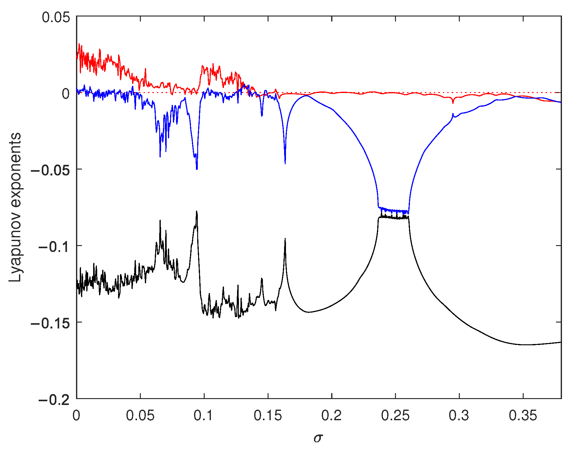
Figure 2 presents the Lyapunov exponent spectrum of system (10) with respect to the parameter $\sigma$. The exponents are computed using the Wolf algorithm along the simulated trajectories. It can be observed that the maximum Lyapunov exponent becomes positive in certain parameter intervals, which indicates the presence of chaotic dynamics. In contrast, when all Lyapunov exponents are non-positive, the system exhibits periodic or stable behavior. The variation in the Lyapunov exponent with respect to $\sigma$ further confirms the transition between different dynamical regimes, which is consistent with the bifurcation analysis.

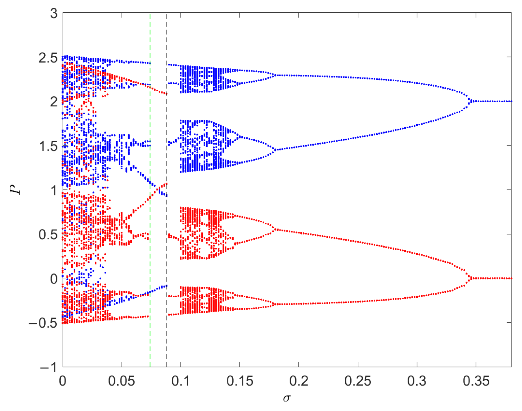
Figure 3 illustrates the bifurcation diagrams of P with respect to $\sigma$ near $E_{+}$ and $E_{-}$. The blue and red diagrams correspond to trajectories evolving around $E_{+}$ and $E_{-}$, respectively. The two diagrams exhibit a symmetric structure and appear as mirror images with respect to the line $P=1$, which corresponds to the normal equilibrium $E_c(1,1,1)$.

In the following theorem, the Hopf bifurcation points around $E_{\pm }$ are determined analytically and verified numerically.

Theorem 2.

With σ as the bifurcation parameter, the following statements hold: (1) If $\sigma >0.34307$, the equilibria $E_{\pm }$ are asymptotically stable. (2) If $\sigma =0.34307$, the equilibria $E_{\pm }$ undergo Hopf bifurcation.

Proof. 

Due to the symmetry of the phase space, it suffices to consider the equilibrium $E_{+}$. The Jacobian matrix evaluated at $E_{+}$ is

$$J(E_{+})=\left(\begin{array}{ccc}-0.1& 0.5& 0.4\\ 0& 0& 0.2\\ 0.1\sigma -0.1& 0.1-0.5\sigma & -0.2\sigma \end{array}\right).$$

(20)

The corresponding characteristic polynomial is

$$f(\lambda )={\lambda }^3+(0.1+0.2\sigma ){\lambda }^2+(0.02+0.08\sigma )\lambda +0.008=0.$$

(21)

Let $p_1=0.1+0.2\sigma ,p_2=0.02+0.08\sigma ,p_3=0.008$. According to the Routh–Hurwitz criterion, the equilibrium $E_{+}$ is locally asymptotically stable if and only if $p_1>0,p_1{p}_2-p_3>0,p_3>0$. From these conditions we obtain $\sigma >0.34307$. Therefore, system (10) is asymptotically stable around $E_{+}$ when $\sigma >0.34307$. Next, assume that Equation (21) admits a pair of purely imaginary eigenvalues ${\lambda }_{1,2}=\pm \omega i,$ where $\omega >0$ denotes a positive quantity depending on the system parameters. Substituting $\lambda =\omega i$ into Equation (21) yields

$$-{\omega }^{3}i-(0.1+0.2\sigma ){\omega }^2+(0.02+0.08\sigma )\omega i+0.008=0.$$

(22)

Separating the real and imaginary parts leads to

$$\left\{\begin{array}{c}-{\omega }^3+(0.02+0.08\sigma )\omega =0,\hfill \\ 0.008-(0.1+0.2\sigma ){\omega }^2=0.\hfill \end{array}\right.$$

(23)

Solving the above equations gives $\sigma =0.34307,\omega =0.21782$. Furthermore, differentiating Equation (21) with respect to $\sigma$ yields

$$3{\lambda }^2{\displaystyle \frac{d\lambda }{d\sigma }}+0.2{\lambda }^2+2(0.1+0.2\sigma )\lambda {\displaystyle \frac{d\lambda }{d\sigma }}+0.08\lambda +(0.02+0.08\sigma ){\displaystyle \frac{d\lambda }{d\sigma }}=0.$$

(24)

Substituting $\lambda =\pm 0.21782i$, $\sigma =0.34307$, gives $\mathrm{Re}\left(\frac{d\lambda }{d\sigma }\right)=-0.0353<0$. Therefore, the transversality condition of Hopf bifurcation is satisfied. Hence, when $\sigma =0.34307$, the equilibrium $E_{+}$ undergoes a Hopf bifurcation. This completes the proof. □

It should be noted that the above bifurcation results are obtained under specific parameter settings and mainly illustrate representative dynamical behaviors of the system, rather than providing a general analytical characterization for all parameter configurations. A complete analytical investigation of Hopf bifurcation under general parameter conditions is mathematically challenging and is left for future work.

4. Global Dynamics

In addition to the bifurcation parameter $\sigma$, other parameters such as $\alpha$ and $\beta$ also play important roles in shaping the system dynamics. The parameter $\alpha$ controls the sensitivity of price adjustment to excess demand, and larger values of $\alpha$ tend to amplify price fluctuations and promote the onset of oscillatory behavior. The parameter $\beta$ determines the responsiveness of demand to price variations, and its variation may alter the nonlinear structure of the demand function, thereby influencing the emergence of complex dynamics. Numerical investigations suggest that, although the specific bifurcation thresholds may vary with these parameters, the qualitative behaviors of the system, including multistability and chaos, remain robust within reasonable parameter ranges. These results indicate that the observed dynamics are governed by the intrinsic mechanisms of the model rather than specific parameter choices.

4.1. Dissipativity

In this subsection, the coefficient of the marginal feedback term $\sigma$ is still treated as the main parameter. The relationship between dissipativity and $\sigma$ is analyzed theoretically. The Jacobian matrix of system (10) is

$$J=\left(\begin{array}{ccc}-{\delta }_2& {\delta }_1& \gamma \\ 0& 0& \Theta \\ {\delta }_2\sigma -\alpha & \alpha -{\delta }_1\sigma & \sigma (\Theta -\gamma )\end{array}\right),$$

(25)

where $\Theta ={3\beta {\beta }_1(1-P)}^2-\beta$. Therefore, the divergence of the vector field is $\nabla V=\mathrm{Tr}(J)=\sigma (\Theta -\gamma )-{\delta }_2$.

It is well known that a dynamical system is dissipative if the divergence of its vector field is negative, that is, $\mathrm{Tr}(J)<0$. In this case, the phase volume contracts exponentially and all trajectories are eventually attracted to a bounded invariant set. When $\mathrm{Tr}(J)=0$, the system becomes conservative. In this case, the parameters $\sigma$ and P satisfy

$$\sigma ={\displaystyle \frac{{\delta }_2}{{3\beta {\beta }_1(1-P)}^2-(\beta +\gamma )}}.$$

(26)

It should be noted that $P\ne 1\pm \sqrt{\frac{\beta +\gamma }{3\beta {\beta }_1}}$; otherwise, $\Theta =\gamma$, which implies $\mathrm{Tr}(J)=-{\delta }_2<0$, and the system is automatically dissipative.

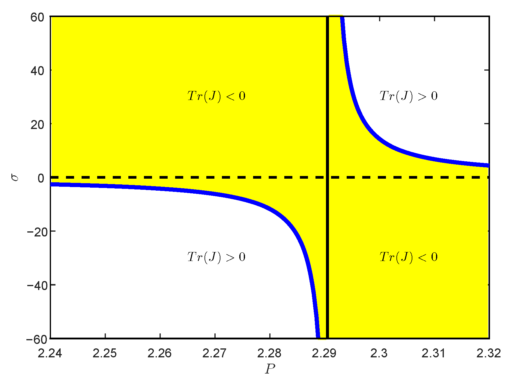
Figure 4 illustrates the dissipative regions of system (10). The system has negative divergence in the yellow region above the dashed line, indicating that the phase volume contracts and the system is dissipative.

From Equation (26), when $P\in \left[\Xi ,1+\sqrt{\frac{\beta +\gamma }{3\beta {\beta }_1}}\right]$, we have $\mathrm{Tr}\left(J\right)<0$ for any $\sigma >0$, where $\Xi =max\left\{0,1-\sqrt{\frac{\beta +\gamma }{3\beta {\beta }_1}}\right\}$. Therefore, the system is dissipative in this price interval regardless of the value of $\sigma$. However, when $P>1+\sqrt{\frac{\beta +\gamma }{3\beta {\beta }_1}}$, the dissipativity condition becomes more restrictive. In this case, $\sigma$ must satisfy $0<\sigma <\frac{{\delta }_2}{\Theta -\gamma }$. This implies that the admissible interval of $\sigma$ shrinks rapidly as P increases. In other words, the Lebesgue measure of the feasible parameter region tends to zero when the price becomes sufficiently large. From an economic perspective, the market system is dissipative most of the time, since commodity prices do not increase without bound in real markets.

4.2. Multistability and Basins of Attraction

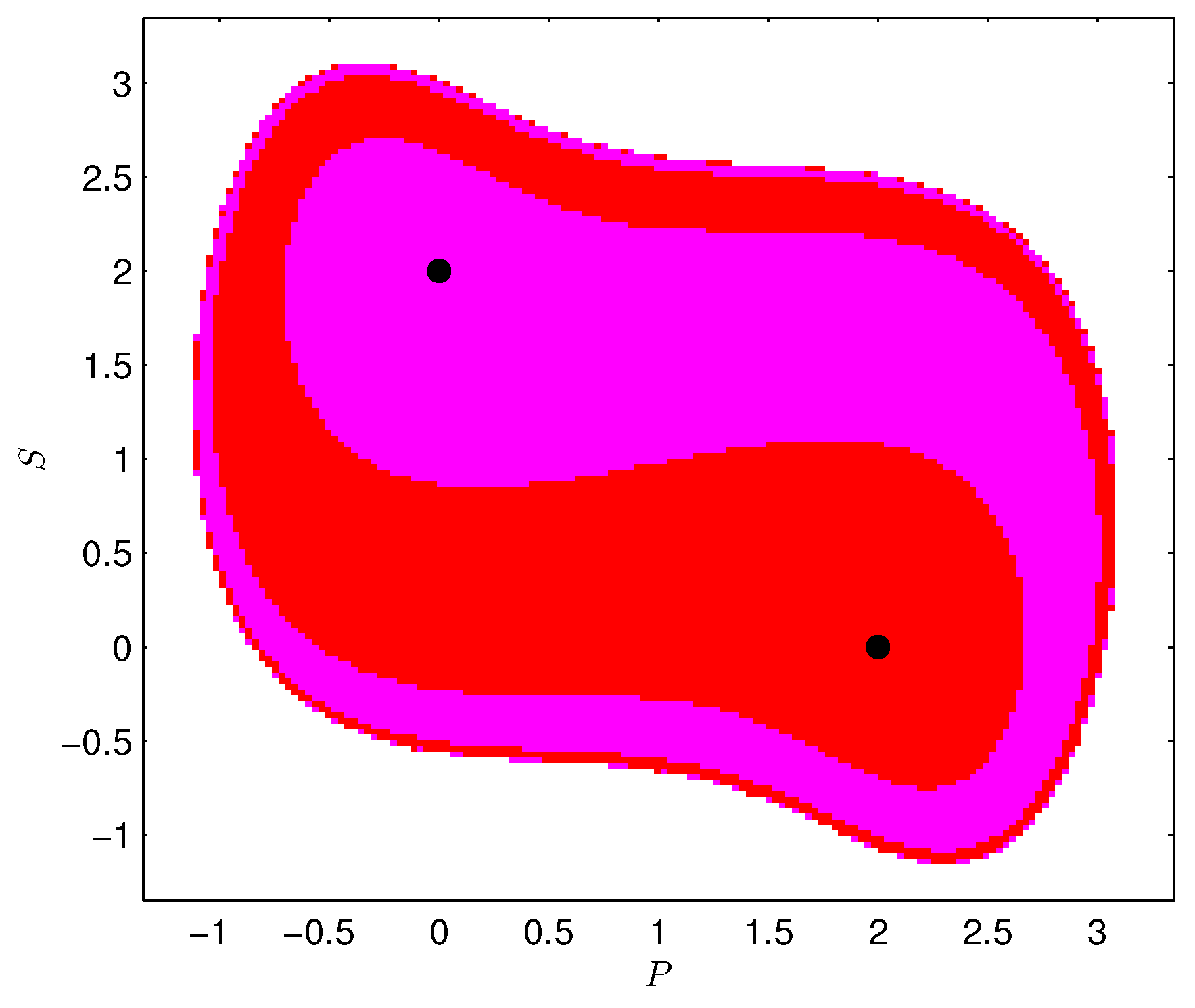
The bifurcation diagrams in Figure 3 indicate that, as the parameter $\sigma$ varies continuously, infinitely many pairs of coexisting attractors may appear, including pairs of chaotic attractors. For convenience, the limit cycles around $E_{-}$ and $E_{+}$ are denoted by $L_{-}$ and $L_{+}$, respectively, while the chaotic attractors around these equilibria are denoted by $C_{-}$ and $C_{+}$. When $\sigma =0.35$, the equilibria $E_{\pm }$ are asymptotically stable focus–nodes, whereas $E_c$ becomes an unstable saddle–focus. Figure 5 presents the basins of attraction for the coexisting point attractors $E_{\pm }$ on the P–S plane with the cross-section $S=D$. The red region corresponds to trajectories converging to $E_{+}(0,0,2)$, while the magenta region corresponds to trajectories converging to $E_{-}(2,2,0)$. Initial states located in the white region lead to trajectories that diverge to infinity. The basins of attraction for the two equilibria are clearly separated and exhibit symmetry with respect to the normal equilibrium $E_c$.

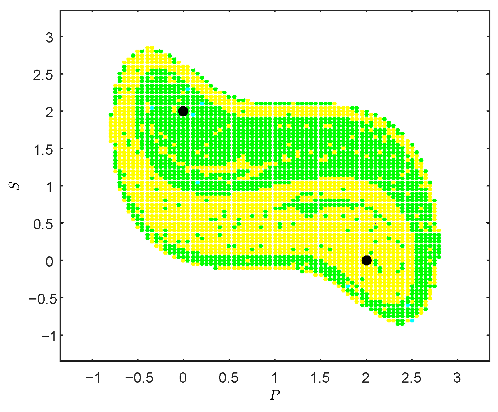
The breaks in the bifurcation diagrams around $\sigma \approx 0.088$ indicate that, as $\sigma$ increases gradually, initial conditions that originally belonged to the basin of one limit cycle may shift into the basin of another limit cycle. Figure 6 shows the basins of attraction for the coexisting limit cycles $L_{\pm }$ when $\sigma =0.095$. It can be observed that the basins of attraction for $L_{-}$ and $L_{+}$ are intertwined and partially diffused. The blurred boundary between these basins implies that small perturbations in $\sigma$ or in the initial conditions may lead to completely different long-term behaviors. For example, when $\sigma$ is slightly smaller than the critical value $\sigma \approx 0.088$, trajectories starting from the initial conditions $(0.1,0.1,0.2)$ and $(1.9,1.9,1.8)$ evolve toward the invariant limit cycles $L_{-}$ and $L_{+}$, respectively. However, when $\sigma$ exceeds this critical value, the roles of the two basins exchange: $L_{-}$ is generated from $(1.9,1.9,1.8)$, while $L_{+}$ originates from $(0.1,0.1,0.2)$.

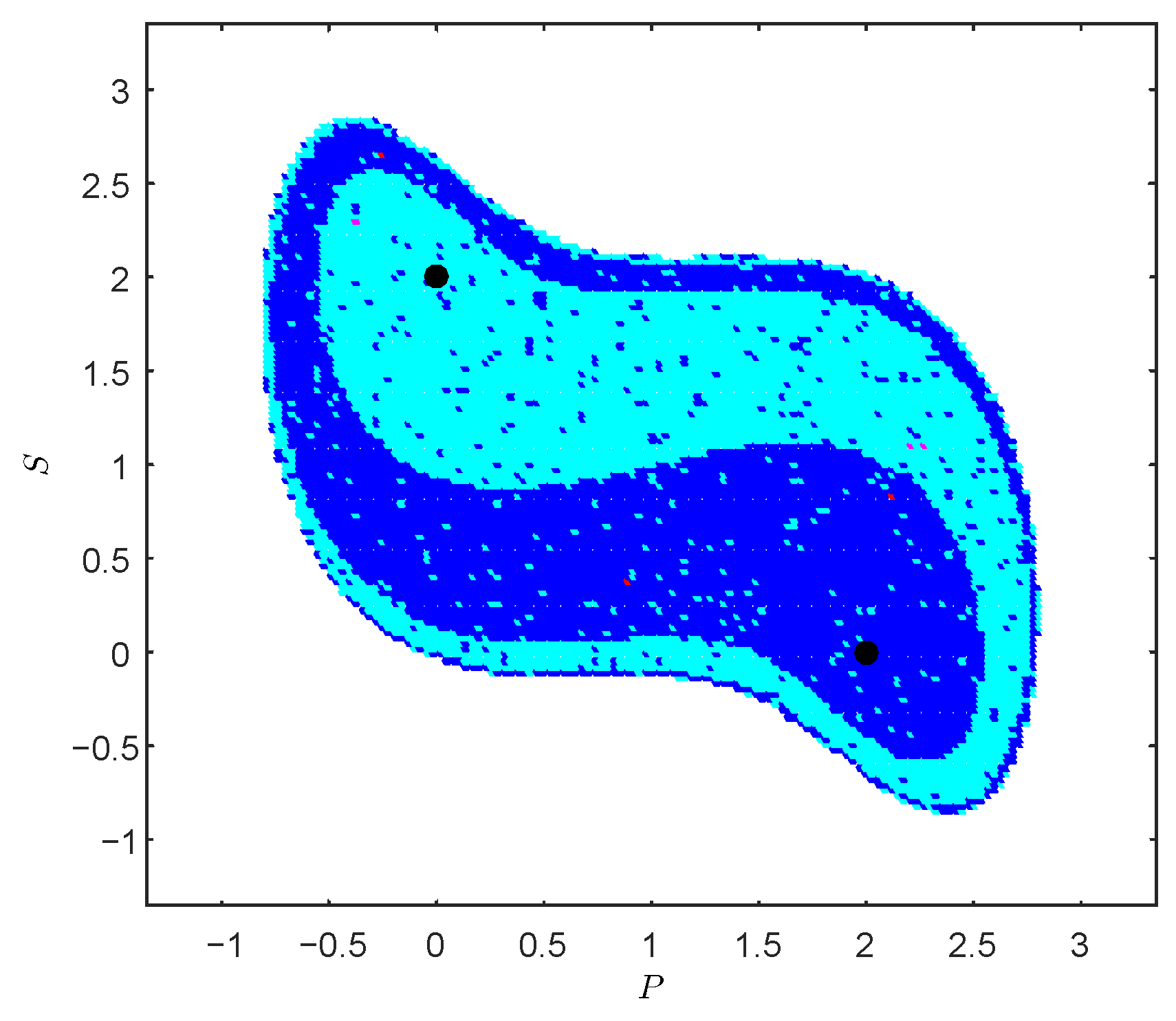
When $\sigma =0.1$, system (10) exhibits a pair of symmetric coexisting chaotic attractors $C_{\pm }$. The corresponding basins of attraction are illustrated in Figure 7. Initial conditions located in the blue region eventually evolve toward the chaotic attractor $C_{+}$, while those in the cyan region converge to $C_{-}$. Interestingly, the basins of attraction for the chaotic attractors do not exhibit a clear boundary. This indicates that trajectories starting near $E_{-}(2,2,0)$ may eventually enter the chaotic attractor $C_{+}$ located around $E_{+}(0,0,2)$, even though their initial states are closer to $E_{-}$. A few isolated points appearing in Figure 7 are caused by numerical errors during the simulation.

The presence of multistability together with intertwined and diffused basins of attraction reveals the high sensitivity of system (10) to both parameters and initial conditions. As $\sigma$ decreases gradually, not only do the geometrical structures of the coexisting attractors change, but the boundaries between their basins also become increasingly blurred and interwoven. Such deformation and diffusion of basin boundaries further enhance the instability and unpredictability of the dynamical behavior of system (10).

To provide a quantitative description of the basins of attraction, we compare the relative areas occupied by different attractors under representative parameter settings. The results indicate that the dominance of attractors varies with the parameter $\sigma$, reflecting the evolution of the basin structures. It should be noted that the present study mainly focuses on qualitative features of basin geometry. A more detailed quantitative analysis, such as the computation of fractal dimensions or boundary complexity, requires more sophisticated numerical methods and is left for future research.

4.3. Splitting of Chaotic Attractors

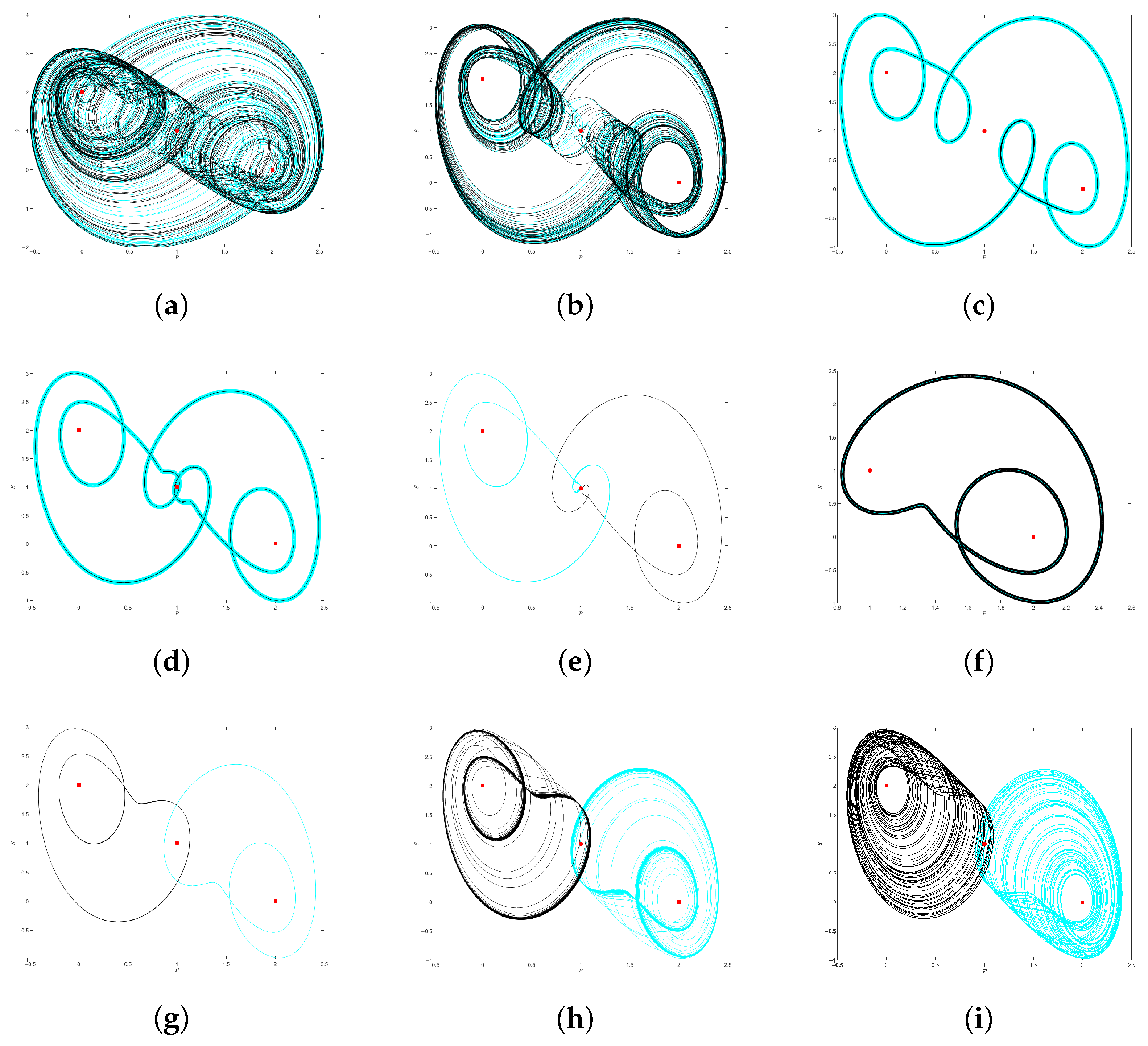
Chaotic attractors with variable numbers of wings have attracted considerable attention in recent studies [15,25]. In this subsection, we investigate how the structure of chaotic attractors in the supply–demand–price model evolves with respect to the parameter $\sigma$. From the bifurcation diagrams in Figure 3, it can be observed that the system exhibits chaotic behavior at both $\sigma =0.1$ and $\sigma \approx 0.02$. However, the fluctuation ranges of the price variable P differ significantly. When $\sigma =0.1$, the chaotic motion oscillates around a single equilibrium ($E_{+}$ or $E_{-}$), whereas for $\sigma \approx 0.02$, the trajectory alternates between the neighborhoods of both equilibria $E_{\pm }$. This indicates that the geometry and extent of chaotic attractors are highly sensitive to the parameter $\sigma$. In particular, a symmetric double-wing chaotic attractor is observed when $\sigma \approx 0.02$, while a pair of coexisting single-wing chaotic attractors emerges when $\sigma \approx 0.1$, as shown in Figure 8a,i. To further understand the transition between these two regimes, we analyze the dynamical evolution of the system over the interval $\sigma \in [0,0.1]$, as illustrated in Figure 8. When $\sigma \approx 0.02$, the system exhibits a double-wing chaotic attractor. As $\sigma$ increases, the attractor gradually evolves into a periodic orbit, as shown in Figure 8b,c. Figure 8a–d demonstrate a transition from double-wing chaos to a limit cycle. Although the phase trajectories in the P–S projection appear to intersect near $E_c$, no actual intersection occurs in the full three-dimensional phase space. When $\sigma \approx 0.074$, the limit cycle splits into a pair of coexisting two-periodic limit cycles, consistent with the bifurcation diagrams in Figure 3. As $\sigma$ increases further beyond $\sigma \approx 0.088$, the positions of the two limit cycles corresponding to different initial conditions interchange due to the distortion of the basins of attraction (see Figure 8e,g). For instance, the trajectory starting from $(0.1,0.1,0.2)$ converges to the limit cycle $L_{-}$ around $E_{-}$ when $\sigma =0.074$ but transitions to the limit cycle $L_{+}$ around $E_{+}$ when $\sigma =0.095$. During this process, temporary overlaps of coexisting limit cycles may appear due to numerical errors, as shown in Figure 8f. When $\sigma$ further increases to $\sigma =0.1$, a pair of symmetric coexisting chaotic attractors emerges. Throughout this transition, the equilibria $E_{\pm }$ and $E_c$ remain unstable saddle–focus points. Specifically, the equilibria $E_{\pm }$ have one-dimensional stable manifolds and two-dimensional unstable manifolds, while $E_c$ has two-dimensional stable manifolds and one-dimensional unstable manifolds. The transition from double-wing chaos to single-wing chaos observed in Figure 8 is obtained from numerical simulations and provides a qualitative description of the evolution of chaotic attractors. Such transitions may be associated with classical routes to chaos, including period-doubling cascades or the emergence of periodic windows, as well as attractor splitting or merging mechanisms. However, a rigorous identification of the underlying mechanism requires a more detailed bifurcation analysis and remains an open problem.

The transition route of chaotic attractors reveals that the breaks in the bifurcation diagrams play a crucial role in the splitting process of chaotic attractors. In particular, the first break around $\sigma \approx 0.074$ corresponds to the splitting of the limit cycle, while the second break around $\sigma \approx 0.088$ corresponds to a change in the $\omega$-limit sets induced by the distortion of the basins of attraction. The observed breaks in the bifurcation diagrams may be related to global bifurcation phenomena. In particular, such abrupt transitions could be associated with boundary crises or attractor merging, where significant changes in the geometry of basins of attraction occur. It should be emphasized that the above interpretation is qualitative in nature and is based on numerical observations. A rigorous identification and classification of the underlying global bifurcations require further theoretical analysis and remain an open problem.

4.4. Endogenous Chaos

In this subsection, we investigate the dynamical systems generated by different orders of derivatives of system (10). Numerical simulations show that the number and geometric structures of chaotic attractors derived from the system are much richer than the two commonly observed types of chaotic attractors. The initial conditions of higher-order derivative systems are determined in a consistent manner from the initial state of the original system. Specifically, given the initial condition $\left(S\right(0),D(0),P(0\left)\right)$ of system (10), the initial values of the first-order derivative system $(\dot{S}(0),\dot{D}(0),\dot{P}(0))$ are obtained by substituting $\left(S\right(0),D(0),P(0\left)\right)$ into the right-hand side of system (10). Higher-order initial conditions, such as $(\ddot{S}(0),\ddot{D}(0),\ddot{P}(0))$, are then constructed recursively by differentiating the system equations and evaluating them at $t=0$. Therefore, the initial conditions of all higher-order systems are uniquely determined by the initial state of the original system, ensuring consistency across different derivative orders.

In this paper, the term ‘endogenous chaos’ refers to chaotic attractors generated by higher-order derivative systems derived from the original dynamical system. The term ‘endogenous’ is used to emphasize that the complex dynamics originate from the intrinsic structure of the system itself, rather than from external stochastic inputs or exogenous disturbances. This notion differs from the concept of ‘endogenous economic fluctuations’ in the economics literature, where endogenous dynamics typically arise from internal economic mechanisms such as expectations, feedback, or strategic interactions. In contrast, the present study focuses on the dynamical systems perspective, where higher-order derivatives of the state variables generate new forms of chaotic behavior.

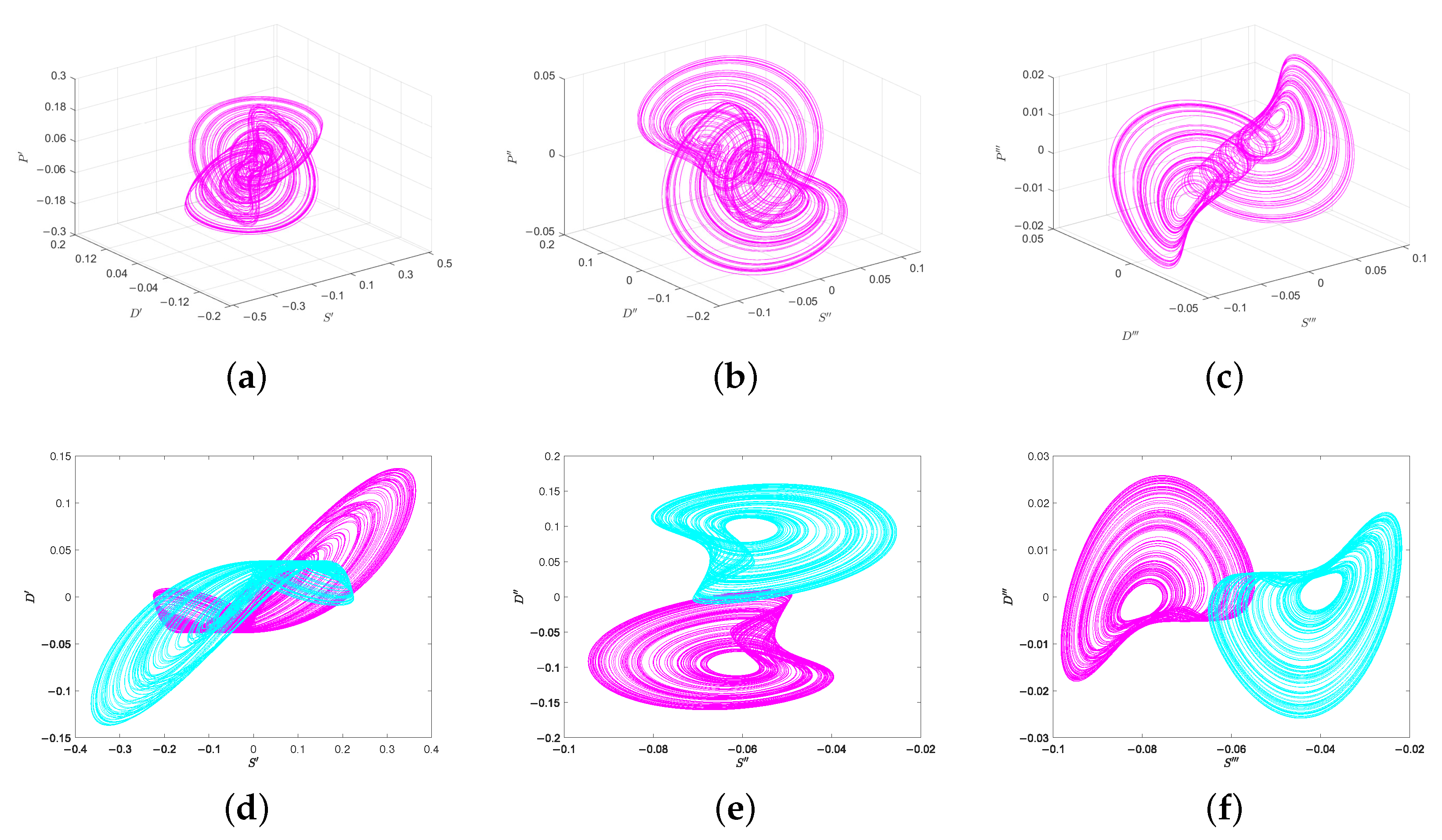
Fix $\sigma =0.02$ and choose the initial conditions $S\left(0\right)=0.1$, $D\left(0\right)=0.1$, and $P\left(0\right)=0.2$. The derivatives $(\dot{S},\dot{D},\dot{P})$ can be computed by substituting the chaotic time series into the right-hand side of system (10). For convenience, the state variable vector $(S,D,P)$ is referred to as the zero-order state system, while the derivative vector $(\dot{S},\dot{D},\dot{P})$ is called the first-order state system. Figure 9a shows that the first-order state system also exhibits chaotic behavior. Moreover, higher-order state systems can be constructed in the same manner, such as the second-order state system $(\ddot{S},\ddot{D},\ddot{P})$ and the third-order state system $(\stackrel{⃛}{S},\stackrel{⃛}{D},\stackrel{⃛}{P})$, as illustrated in Figure 9b,c. These derived systems exhibit different forms of chaotic attractors.

Inspired by the concept of endogenous dynamics in economics, the chaotic attractors generated by derivative systems of order greater than zero are collectively referred to as endogenous chaotic attractors. To the best of our knowledge, this phenomenon has not been extensively investigated in the literature. There exist intrinsic relationships between endogenous chaotic attractors and the chaotic attractor of the zero-order system. First, each endogenous system is essentially a linear or nonlinear combination of the state variables $(S,D,P)$ of the zero-order system. Therefore, the chaotic property of the time series is preserved under derivative operations and nonlinear coupling. Second, the phase portraits of system (10) are symmetric with respect to the equilibrium point $E_c$, and the endogenous chaotic attractors are also centrally symmetric. However, the symmetry center becomes the origin $O(0,0,0)$, because the vector field of the zero-order system vanishes at the equilibria $E_c$, $E_{+}$, and $E_{-}$. Consequently, $O(0,0,0)$ is an equilibrium point for all endogenous derivative systems.

Another interesting observation is that the size of the endogenous chaotic attractors decreases gradually as the derivative order increases, as shown in Figure 9a–c. To explain this phenomenon, consider the general dynamical system

$$\dot{w}=f(w),w\in C^{\infty }(\mathbb{R},{\mathbb{R}}^n),f\in C^{\infty }({\mathbb{R}}^n,{\mathbb{R}}^n).$$

(27)

Suppose that $w^{*}$ is an equilibrium point of system (27). Linearizing system (27) at $w=w^{*}$ gives

$$\dot{w}=f(w^{*})+{\displaystyle \frac{\partial f}{\partial w^{*}}}(w-w^{*})+o({\parallel w-w^{*}\parallel }^2)=J_{w^{*}}(w-w^{*})+o({\parallel w-w^{*}\parallel }^2),$$

(28)

where $J_{w^{*}}$ denotes the Jacobian matrix evaluated at $w^{*}$. Neglecting higher-order terms yields the approximate linear relationship

$$\dot{w}=J_{w^{*}}(w-w^{*}).$$

(29)

By repeatedly applying the chain rule, two systems whose derivative orders differ by one approximately satisfy

$$w^{(n+1)}=J_{w^{*}}{w}^{\left(n\right)},n\in {\mathbb{N}}^{+},$$

(30)

where the superscript denotes the derivative order. Therefore,

$${\displaystyle \frac{\parallel w^{(n+1)}\parallel }{\parallel w^{\left(n\right)}\parallel }}\le \parallel J_{w^{*}}\parallel ,$$

(31)

where $\parallel ·\parallel$ denotes a matrix norm. This inequality indicates that the size ratio between two chaotic attractors whose derivative orders differ by one is bounded by $\parallel J_{w^{*}}\parallel$.

It should be noted that Equation (30) is derived based on a linearization of the system around the equilibrium point $w^{*}$ and therefore is only valid as a local approximation. This relation is used to provide qualitative insight into the scaling behavior between successive derivative systems. However, for trajectories evolving far from equilibrium, especially in chaotic regimes, higher-order nonlinear terms may play a significant role, and the approximation in Equation (30) may no longer be accurate. A rigorous global characterization of this relationship remains an open problem and is beyond the scope of the present study.

For the model studied in this paper, if $w^{*}$ corresponds to the equilibrium $E_c$, the Frobenius norm of the Jacobian matrix is $\parallel J_{w^{*}}\parallel =0.6692<1$. This explains why the size of endogenous chaotic attractors decreases as the derivative order increases. Moreover, the motion region of the attractors tends to shrink toward the origin as the derivative order becomes sufficiently large. Another interesting phenomenon is that the coexistence of chaotic attractors observed in the zero-order system is inherited by the endogenous systems. When $\sigma =0.1$, the zero-order system exhibits a pair of coexisting chaotic attractors. Figure 9d–f show that corresponding pairs of endogenous chaotic attractors also appear in the first-, second-, and third-order derivative systems. These coexisting attractors remain symmetric with respect to the origin $O(0,0,0)$. Note that the initial values of the endogenous systems are determined by the initial state of the zero-order system. These observations suggest that endogenous chaotic attractors may be a widespread phenomenon in nonlinear dynamical systems. Once a dynamical system generates a chaotic attractor, infinitely many endogenous chaotic attractors of higher derivative orders may be constructed.

It should be noted that the higher-order derivative systems do not necessarily preserve chaotic behavior under all conditions. Although the numerical results presented in this paper demonstrate that low-order derivative systems can inherit chaotic dynamics from the original system, different derivative orders and parameter settings may also lead to periodic or convergent behavior. A systematic investigation of the dynamical properties across different derivative orders remains an interesting topic for future research.

5. Application

As a practical application of the proposed model, real-world data are employed to identify the parameters of system (10) and to evaluate its effectiveness. Since the model is formulated as a continuous-time dynamical system, a discretization procedure is required for empirical data fitting. In this study, the system is discretized using the forward Euler method with a sufficiently small time step to ensure numerical stability and accuracy. The step size is selected such that further reduction does not lead to significant changes in the simulation results, indicating that the discretization error is well controlled and does not affect the main conclusions.

For parameter identification, we consider the general system (27) and construct a corresponding discrete-time approximation. Specifically, the continuous system is transformed into the following iterative form:

$$w_{k+1}=w_k+f(w_k):=F(w_k,p),$$

(32)

where p denotes the parameter vector, and $F(w_k,p)\in C({\mathbb{R}}^n,{\mathbb{R}}^n)$ represents the prediction map used for data fitting and parameter estimation.

The dataset used in this study is obtained from the International Energy Agency (IEA), which includes quarterly data on global trade oil supply, demand, and WTI crude oil prices from 2006 to 2018. It is well known that supply and demand influence the long-term trend of oil prices. Therefore, the empirical mode decomposition (EMD) method [26] is first employed to extract the long-term trend component of the oil price series, which replaces the original price data in the model. To eliminate the influence of dimensional differences among variables, all data are normalized according to

$$\overline{x}={\displaystyle \frac{x-x_{min}}{x_{max}-x_{min}}},$$

(33)

where $x_{min}$ and $x_{max}$ denote the minimum and maximum values of the data sequence $\left\{x\right\}$, respectively, x is the original data, and $\overline{x}$ is the normalized data.

Parameter identification for vector p in Equation (29) can be formulated as the following optimization problem:

$$\underset{p}{min}\sum _k{\parallel x_{k+1}-F_p(x_k)\parallel }^2.$$

(34)

The genetic algorithm (GA) is employed to estimate the model parameters by minimizing the fitting error. During the optimization process, the objective function exhibits a stable convergence trend as the number of iterations increases. To assess the robustness of the identified parameters, the GA is executed multiple times with different initial populations. The resulting parameter values remain consistent across runs, indicating that the identification results are stable. Moreover, the variation in the identified parameters is relatively small, providing an approximate indication of parameter reliability. The above nonlinear optimization problem is solved using the genetic algorithm, and the estimated parameters are listed in

Table 2. Parameter identification results obtained by the genetic algorithm.

$\mathit{\gamma }$	${\mathit{\delta }}_1$	${\mathit{\delta }}_2$	$\mathit{\beta }$	${\mathit{\beta }}_1$	$\mathit{\alpha }$	$\mathit{\sigma }$	${\mathit{P}}_{\mathit{s}}$	${\mathit{P}}_{\mathit{d}}$
0.00181	0.22703	0.23526	0.06793	0.94210	0.65388	0.07142	0.46110	0.91150

. Based on these results, the analytic form of the prediction map is obtained. In particular, for the model proposed in this paper, the prediction map takes the form

$$F:\left(\begin{array}{c}S\\ D\\ P\end{array}\right)\to \left(\begin{array}{c}-0.00083+0.76474S+0.22703D+0.00181P\\ 0.013454+D+0.09159P-0.17164P^2+0.06029P^3\\ 0.00102+0.63767D-0.67068S+1.00641P-0.01225P^2+0.00431P^3\end{array}\right).$$

(35)

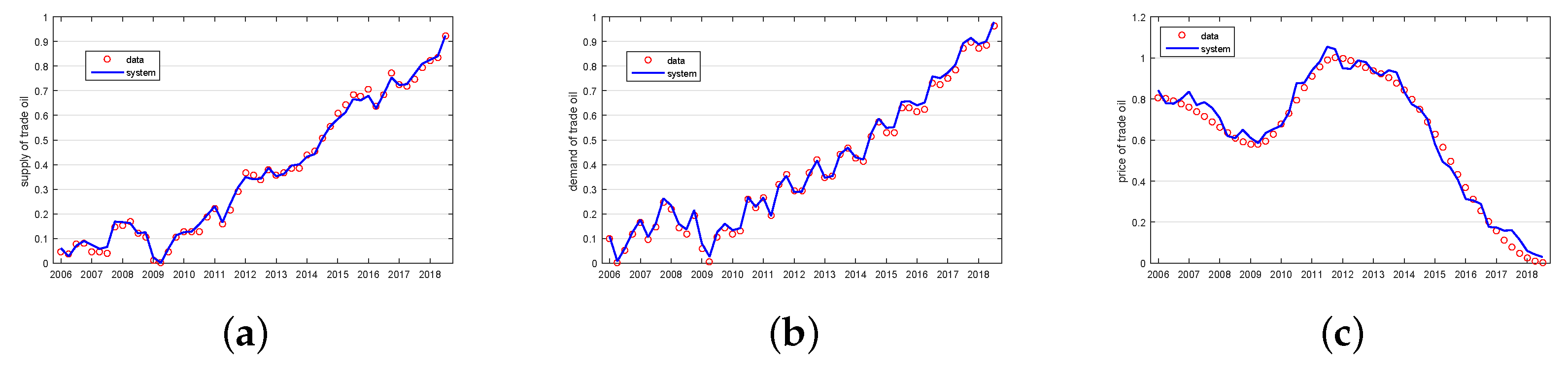
In the prediction process, the k-th group of normalized data is used as the input of the prediction map F, and the output is taken as the predicted value of the $(k+1)$-th group. Figure 10 presents the comparison between the quarterly observed data and the model predictions for global trade oil, including supply, demand, and price. The predicted results closely match the real data, indicating that the proposed model can effectively capture the evolution characteristics of the oil market dynamics.

To quantitatively evaluate the fitting performance, the root mean square error (RMSE) is computed between the model output and the empirical data. The RMSE is defined as

$$\mathrm{RMSE}=\sqrt{{\displaystyle \frac{1}{N}}\sum _{k=1}^N{\left(x_k^{\mathrm{model}}-x_k^{\mathrm{data}}\right)}^2}.$$

(36)

The estimated RMSE is approximately $0.082$, indicating a good agreement between the model and the observed data.

6. Conclusions

This paper investigates the complex dynamics of a supply–demand–price model with a marginal feedback term that reflects the panic expectations of individuals. The dynamical behaviors of the system, including stability, Hopf bifurcation, chaotic attractors, and multistability, are analyzed through phase portraits, bifurcation diagrams, Lyapunov exponents, and basins of attraction. The results show that when the suppression intensity of supply exceeds the incentive intensity of demand, the market can reach a stable equilibrium; otherwise, the market becomes unstable. Moreover, the coefficient of the marginal feedback term plays a crucial role in determining market dynamics. When this coefficient is relatively large, the market fluctuates around a single equilibrium with either collectability or saturation depending on the initial conditions, indicating strong path dependence. In contrast, when the coefficient is relatively small, the system may fluctuate around two equilibria corresponding to collectability and saturation. The breaks observed in the bifurcation diagrams suggest that the distortion and diffusion of basins of attraction can destabilize the market, providing a possible explanation for sudden changes in price dynamics. Finally, the endogenous chaotic attractors of the system are examined. It is found that the endogenous system exhibits symmetric chaotic attractors as well as coexisting chaotic attractors, and the threshold for the ratio of the sizes of two chaotic attractors differing by one order is theoretically analyzed.

From a theoretical perspective, the introduction of marginal feedback extends classical supply–demand–price models by incorporating higher-order dynamical effects, providing a new mechanism to explain complex phenomena such as multistability and endogenous chaos. This contributes to bridging traditional economic models and nonlinear dynamical systems. From a managerial perspective, the results suggest that not only the magnitude of supply–demand imbalance but also its rate of change plays a crucial role in market dynamics. Rapid variations in market conditions may significantly amplify price fluctuations. Therefore, policymakers and market regulators should monitor both the level and the variation speed of excess demand in order to better anticipate and mitigate market instability.

Despite these contributions, several limitations should be noted. First, the model is formulated as a deterministic system and does not account for stochastic disturbances or external shocks. Second, the theoretical analysis is mainly conducted under specific parameter settings, and a complete analytical characterization for general parameter regimes remains challenging. Third, the empirical validation relies on a single dataset, which may limit the general applicability of the results.

Future research may proceed in several directions. First, stochastic effects and external perturbations can be incorporated to better reflect real market environments. Second, the model can be extended to networked or multi-market systems to investigate interactions among multiple agents or commodities. Third, more general analytical conditions for bifurcation and global dynamics could be developed. Finally, further empirical validation using diverse datasets and advanced parameter identification methods would enhance the robustness and applicability of the proposed model.

References

1. Kjellberg, H.; Sjogren, E.; Krafve, L.J. The functions of known to be inaccurate prices in markets: A cross-country comparison of pharmaceutical list pricing. J. Bus. Res. 2023, 167, 114193. [Google Scholar] [CrossRef] [Scilit]
2. Bossley, L. The mythical market price of oil. J. World Energy Law Bus. 2026, 19, Jwag002. [Google Scholar] [CrossRef] [Scilit]
3. Sun, T.H.; Huang, N.; Jiang, W.J. From carbon policy to public health: An analysis of pricing decisions in electronics supply chains for costing emissions reduction. Front. Public Health 2026, 14, 1723064. [Google Scholar] [CrossRef] [Scilit]
4. Lin, Z.; Li, P.; Zhao, Z.; Wang, F.; Zhou, T.; Cao, C. FATE-Net: An optimization-enhanced attention-driven temporal evolution framework for stock price forecasting. Mathematics 2026, 14, 964. [Google Scholar] [CrossRef] [Scilit]
5. Du, J.D.; Cao, W.Y.; Wang, Z.Y. Forecasting risk matrices with economic policy uncertainty and financial stress: A machine learning approach. Mathematics 2026, 14, 938. [Google Scholar] [CrossRef] [Scilit]
6. Wang, Y.; Pan, M.; Qi, X.; Liu, J.; Wang, Y.; Ju, L. Dynamic bilevel optimization of market participation and strategic bidding in renewable-dominated electricity markets. Energies 2026, 19, 1285. [Google Scholar] [CrossRef] [Scilit]
7. Lin, H.L.; Dai, L. Adaptive subsidy policies for shore power promotion: An integrated game theory-system dynamics approach. Mathematics 2026, 14, 860. [Google Scholar] [CrossRef] [Scilit]
8. Zhang, J.Y.; Rosca, E.; Pradhan, P. Unveiling hidden costs in agrifood systems: A systematic review of true cost accounting. Trends Food Sci. Technol. 2026, 171, 105633. [Google Scholar] [CrossRef] [Scilit]
9. Richard, A.; Michel, Q. The Economics of Alfred Marshall; Palgrave Macmillan: London, UK, 2003. [Google Scholar]
10. Hommes, C. Behavioral and experimental macroeconomics and policy analysis: A complex systems approach. J. Econ. Lit. 2021, 59, 149–219. [Google Scholar] [CrossRef] [Scilit]
11. Li, T.; Sun, Z.; Zhou, M.; Sze, N.N.; Zhou, Y. Modeling bounded rationality in pedestrian-vehicle interactions at non-signalized crosswalks: A game theoretic quantal response equilibrium approach. Accid. Anal. Prev. 2026, 231, 108502. [Google Scholar] [CrossRef] [Scilit]
12. Yang, T.; Cheng, Q.; Chen, B.; Lu, D.; Wu, H.; Zhu, Y. Credible reserve assessment method for virtual power plants considering user-bounded rationality response. Sustainability 2026, 18, 3130. [Google Scholar] [CrossRef] [Scilit]
13. Li, D.D.; Han, S. Evolutionary dynamics of cooperation with tolerance and historical payoff memory in the prisoner’s dilemma. Chaos Solitons Fractals 2026, 208, 118322. [Google Scholar] [CrossRef] [Scilit]
14. Anzo-Hernández, A.; Gilardi-Velazquez, H.E.; Campos-Canton, E. On multistability behavior of unstable dissipative systems. Chaos 2018, 28, 033613. [Google Scholar] [CrossRef] [Scilit]
15. Kengne, J.; Njikam, S.M.; Folifack, V.R. A plethora of coexisting strange attractors in a simple jerk system with hyperbolic tangent nonlinearity. Chaos Solitons Fractals 2018, 106, 201–213. [Google Scholar] [CrossRef] [Scilit]
16. Raza, N.; Moazeni, F. Data-driven identification of chaotic nonlinear systems using local maximum entropy surrogates. Nonlinear Dyn. 2026, 114, 467. [Google Scholar] [CrossRef] [Scilit]
17. Zhu, W.; Luo, Y.; Cao, J.; Yue, D. Impulsive edge event-triggered sliding mode consensus control of second-order nonlinear multi-agent systems. Commun. Nonlinear Sci. Numer. Simul. 2026, 160, 109951. [Google Scholar] [CrossRef] [Scilit]
18. Hua, Z.; Yang, C.; Yan, X.; Jia, F.; Zhang, Q. Global predefined-time neural network exact tracking for high-order nonlinear systems with time-varying delay. Nonlinear Dyn. 2026, 114, 493. [Google Scholar] [CrossRef] [Scilit]
19. Chaudhry, M.I.; Miranda, M.J. Complex price dynamics in vertically linked cobweb markets. Econ. Model. 2018, 72, 363–378. [Google Scholar] [CrossRef] [Scilit]
20. Chaudhry, M.I.; Miranda, M.J. Endogenous price fluctuations: Evidence from the chicken supply chain in Pakistan. Am. J. Agric. Econ. 2024, 106, 637–658. [Google Scholar] [CrossRef] [Scilit]
21. Guse, E.; Wong, M.C.S. Communication and learning: The bilateral information transmission in the cobweb model. Comput. Econ. 2022, 60, 693–723. [Google Scholar] [CrossRef] [Scilit]
22. Cavalli, F.; Naimzada, A.K.; Pecora, N.; Pireddu, M. Agents’ beliefs and economic regimes polarization in interacting markets. Chaos 2018, 28, 055911. [Google Scholar] [CrossRef] [Scilit] [PubMed]
23. Li, Y.C.; Yang, H. A mathematical model of demand-supply dynamics with collectability and saturation factors. Int. J. Bifurc. Chaos 2017, 27, 1750016. [Google Scholar] [CrossRef] [Scilit]
24. Sun, M.; Tian, L.; Fu, Y. An energy resources demand–supply system and its dynamical analysis. Chaos Solitons Fractals 2007, 32, 168–180. [Google Scholar] [CrossRef] [Scilit]
25. Zhang, S.; Zeng, Y.; Li, Z.; Wang, M.; Xiong, L. Generating one to four-wing hidden attractors in a novel 4D no-equilibrium chaotic system with extreme multistability. Chaos 2018, 28, 013113. [Google Scholar] [CrossRef] [Scilit] [PubMed]
26. Li, D.; Feng, Y.R.; Yan, X.Y. An integrated prediction framework combining variational mode optimization decomposition, empirical quantile regression, and QLattice for dynamic point and interval prediction of carbon prices. Energy 2026, 348, 140372. [Google Scholar] [CrossRef] [Scilit]
Figure 1. Framework of the proposed methodology, including model construction, theoretical analysis, numerical simulations, extended analysis, and empirical validation.
Mathematics 14 01337 g001
Figure 2. Lyapunov exponent spectrum of system (10) as a function of the parameter σ . The exponents are computed using the Wolf algorithm. Positive values of the maximum Lyapunov exponent indicate chaotic behavior, while non-positive values correspond to periodic or stable dynamics.
Mathematics 14 01337 g002
Figure 3. Bifurcation diagrams of P with respect to σ . The red and blue diagrams correspond to the initial conditions S ( 0 ) = 0.1 , D ( 0 ) = 0.1 , P ( 0 ) = 0.2 and S ( 0 ) = 1.9 , D ( 0 ) = 1.9 , P ( 0 ) = 1.8 , respectively. The bifurcation diagrams break near the green and black dashed lines, where σ 0.074 (green) and σ 0.088 (black).
Mathematics 14 01337 g003
Figure 4. Dissipative regions of system (10). The divergence is negative in the yellow regions and vanishes along the blue curves. The black solid line represents P = 1 + β + γ 3 β β 1 2.291 , while the dashed line corresponds to σ = 0 . The parameters are fixed as α = 0.1 , β = 0.1 , β 1 = 1 , δ 1 = 0.5 , δ 2 = 0.1 , γ = 0.4 , P s = 2 , P d = 1 .
Mathematics 14 01337 g004
Figure 5. Cross-section ( S = D ) of the basins of attraction for the coexisting point attractors when σ = 0.35 . The basins converging to E + are shown in red, while those converging to E are shown in magenta. Trajectories originating from the white region diverge to infinity. Parameters are fixed as α = 0.1 , β = 0.1 , β 1 = 1 , δ 1 = 0.5 , δ 2 = 0.1 , γ = 0.4 , P s = 2 , P d = 1 .
Mathematics 14 01337 g005
Figure 6. Cross-section ( S = D ) of the basins of attraction for the coexisting limit cycles when σ = 0.095 . The basins corresponding to L + are shown in yellow and those corresponding to L are shown in green. White regions correspond to divergent trajectories. Parameters are fixed as α = 0.1 , β = 0.1 , β 1 = 1 , δ 1 = 0.5 , δ 2 = 0.1 , γ = 0.4 , P s = 2 , P d = 1 .
Mathematics 14 01337 g006
Figure 7. Cross-section ( S = D ) of the basins of attraction for the coexisting chaotic attractors when σ = 0.1 . The basins of C + are shown in blue and those of C are shown in cyan. White regions correspond to divergent trajectories. Parameters are fixed as α = 0.1 , β = 0.1 , β 1 = 1 , δ 1 = 0.5 , δ 2 = 0.1 , γ = 0.4 , P s = 2 , P d = 1 .
Mathematics 14 01337 g007
Figure 8. Cross-sections ( S = D ) of the dynamics on the PS plane as σ varies. (a) σ = 0 . (b) σ = 0.04 . (c) σ = 0.043 . (d) σ = 0.07 . (e) σ = 0.074 . (f) σ = 0.09 . (g) σ = 0.095 . (h) σ = 0.09812 . (i) σ = 0.1 . Cyan trajectories originate from ( 0.1 , 0.1 , 0.2 ) , and black trajectories originate from ( 1.9 , 1.9 , 1.8 ) . Red squares denote E ± and the red circle denotes E c . Parameters are fixed as α = 0.1 , β = 0.1 , β 1 = 1 , δ 1 = 0.5 , δ 2 = 0.1 , γ = 0.4 , P s = 2 , P d = 1 .
Mathematics 14 01337 g008
Figure 9. Phase portraits of endogenous chaos. (a) First-order endogenous chaotic system. (b) Second-order endogenous chaotic system. (c) Third-order endogenous chaotic system. (d) First-order coexisting chaotic attractors. (e) Second-order coexisting chaotic attractors. (f) Third-order coexisting chaotic attractors. In (ac), σ = 0.02 ; in (df), σ = 0.1 . In (af), the initial value of the phase portraits in magenta is S ( 0 ) = 0.1 , D ( 0 ) = 0.1 , P ( 0 ) = 0.2 , and the initial value in cyan is S ( 0 ) = 1.9 , D ( 0 ) = 1.9 , P ( 0 ) = 1.8 .
Mathematics 14 01337 g009
Figure 10. Comparison between real data and model predictions for global trade oil. (a) Supply data. (b) Demand data. (c) Price data.
Mathematics 14 01337 g010