Risk-Sensitive Reinforcement Learning for Portfolio Optimization Under Stochastic Market Dynamics

Abstract

Portfolio optimization is one of the most difficult sequential decision problems, as uncertainty and the non-stationary nature of financial markets hinder the development of robust strategies. Reinforcement learning is an attractive framework for addressing this problem, as it allows agents to learn market-adaptive strategies through data-driven interactions. However, existing risk-neutral reinforcement learning solutions for portfolio management are oblivious to downside risk and are mainly concerned with maximizing returns. To address this limitation, this paper proposes a novel risk-sensitive reinforcement learning framework for risk-aware portfolio optimization based on a conditional value-at-risk-based learning objective that explicitly controls extreme loss events. It formulates the portfolio optimization problem as a Markov decision process and solves it using a linearized actor–critic architecture. It also develops theoretical results to analyze important aspects of the learning process, specifically proving that the convexity of the conditional value-at-risk-based formulation and convergence of learning hold under standard assumptions. The proposed algorithm is applied in a realistic investment setting using NIFTY 50 market data. Quantitative results from a rolling window backtesting methodology show that the proposed model achieves the best risk-adjusted portfolio performance, i.e., a Sharpe ratio (0.610), while significantly reducing tail risk, as measured by the conditional value-at-risk (−0.121) and maximum drawdown (−0.198), compared to classical strategies and risk-neutral reinforcement learning solutions. Overall, the results demonstrate that integrating coherent risk measures into reinforcement learning provides an effective approach for developing robust and risk-aware portfolio optimization strategies in dynamic financial environments.

1. Introduction

Portfolio optimization is a fundamental problem in financial decision-making, in which investors seek to allocate capital among multiple assets to achieve an optimal balance between expected return and investment risk [1]. The market setting for portfolio optimization was first mathematically formalized by Markowitz through his mean–variance framework [2]. The explicit formulation of the trade-off between expected return and investment risk has become a fundamental building block of modern portfolio theory [2] and the foundation for a large body of research on portfolio optimization in finance and decision sciences [1,2].

Although this framework is very appealing at the theoretical level, it heavily restricts its practical application, as the optimal weights are assumed to be known at each time step, and the framework is based on very strong assumptions such as normally distributed returns [3], constant market conditions, and fixed investment horizons. These assumptions are too strong for real-life financial applications [3,4]. Financial markets are time-varying and exhibit complex dynamics such as volatility clustering, regime changes, and heavy-tailed return distributions [3]. These characteristics imply that portfolio choices need to be continuously recomputed as market conditions evolve. This leads to a need for sequential decision-making methods that can handle dynamically changing environments and manage uncertainty in a rigorous way.

Reinforcement learning (RL) [5] is a powerful tool for addressing sequential decision-making problems. By integrating portfolio allocation models with RL, it enables agents to learn adaptive investment strategies through interaction with the market environment [6,7,8]. Unlike traditional optimization techniques, RL methods dynamically update portfolio policies [7,8] based on interactions with the investment market, which is often non-stationary [9,10], while at the same time adapting decisions to uncertain market environments. Despite these advantages, most RL approaches in finance are based on a risk-neutral framework [11], focusing primarily on maximizing cumulative returns. While these models can potentially achieve high expected returns, they do not adequately address downside risk and may expose investors to large losses when markets behave unexpectedly [12,13]. In real-world investment scenarios, controlling extreme losses is as important as achieving high returns, highlighting the importance of risk-aware learning frameworks [14].

To overcome this limitation, coherent risk measures such as conditional value-at-risk (CVaR) have attracted significant attention in financial risk management [15,16]. CVaR, as a tail-risk measure, captures risk directly by estimating the expected loss in the worst-case outcomes. As a result, incorporating CVaR into reinforcement learning methodology leads to return-oriented yet robust policies [17]. Although CVaR-based optimization and risk-sensitive reinforcement learning have been investigated separately in the literature, their integration in a stochastic framework is not yet well established. In particular, stochastic differential equations, coherent risk control, and actor–critic learning have not been unified within a single portfolio optimization framework [18].

The proposed method uses a risk-sensitive reinforcement learning framework for portfolio optimization in a stochastic setting. It incorporates CVaR directly into the reinforcement learning objective function and employs an actor–critic architecture to obtain an adaptive allocation policy. By combining stochastic market modeling and coherent risk control, and introducing sequential learning into decision-making, a stochastic market modeling framework is developed for optimal portfolio choice under uncertainty. Furthermore, many RL approaches rely purely on data-driven environments without explicitly modeling underlying market dynamics. In contrast, this approach introduces stochastic market behavior for a more structured and financially relevant representation of asset dynamics. This formulation enables the simultaneous capture of sequential decision-making, tail-risk control, and market uncertainty.

In this article, a preliminary framework for the coherent integration of coherent risk measures, actor–critic learning, and dynamic portfolio rebalancing is introduced. This integration has received relatively little attention in the literature. The main contributions of this article are summarized as follows:

• Propose a risk-sensitive RL framework with CVaR explicitly included in the learning objective to facilitate tail-risk-aware decision-making.
• Combine a reinforcement learning framework with stochastic differential equation- based financial modeling to obtain a financially plausible representation of asset dynamics.
• Propose a novel actor–critic structure that jointly optimizes expected returns and downside risk in a dynamic portfolio optimization setting.
• Provide a theoretical analysis of the proposed framework and establish properties such as convexity and convergence.
• Evaluate the performance on NIFTY 50 data and compare it against classical portfolio strategies as well as risk-neutral RL-based frameworks. The proposed framework achieves superior risk-adjusted returns.

The rest of this paper is structured as follows: Section 2 discusses the literature review and positions our work in the context of related research. Section 3 introduces the problem formulation and the stochastic market model, including notation and portfolio dynamics. Section 4 presents the proposed risk-sensitive reinforcement learning formulation, including the Markov decision process formulation, objective function, and risk-sensitive reinforcement learning algorithm. Section 5 contains the analysis of the proposed method. Section 6 provides the experimental setup and numerical results, including benchmark comparisons and the evaluation metrics used. Section 7 discusses the findings overall and presents the concluding remarks and directions for future work.

2. Literature Review and Problem Positioning

There are three major research directions in portfolio optimization: classical finance models, machine learning-based methods, and reinforcement learning models for sequential decision-making.

2.1. Classical Portfolio Optimization

Classical portfolio optimization is based on the mean–variance framework [1], which models risk via variance of portfolio returns and captures the trade-off between expected return and risk. It leads to a convex optimization problem and the classical efficient frontier, parameterized by risk preferences. It has thus become a central model in financial economics because of its mathematical simplicity and interpretability [1,5].

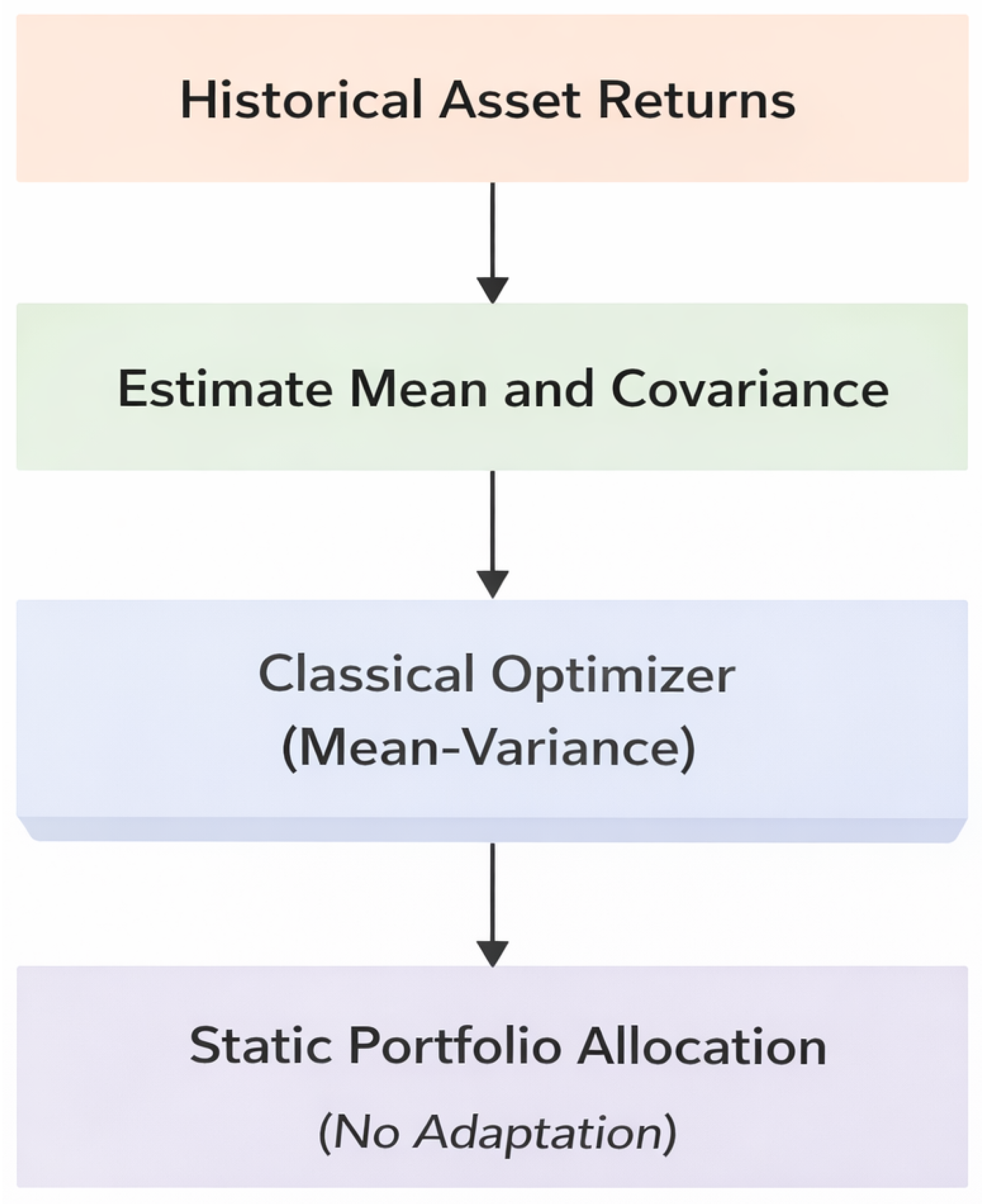
The classical portfolio optimization problem in Figure 1 uses portfolio weights as products of historically estimated expected returns and covariance matrices. Thus, it implicitly assumes a static environment and does not capture adaptive decision processes; it is therefore not fully applicable to dynamic, non-stationary financial environments.

Further developments of the mean–variance paradigm lead to models with continuous time and stochastic calculus. Optimal control theory [10] is used, where the prices of assets are given by stochastic differential equations and optimal policies by dynamic programming [12] or Hamilton–Jacobi–Bellman equations [13]. Such models provide a solid theoretical basis for intertemporal portfolio choice with uncertainty.

Although these methods have many strengths, they rely on simplifying assumptions such as normality of returns, stationarity and time-invariant model parameters. However, financial markets are often characterized by heavy tails, clustering of volatility and regime shifts and thus violate the assumptions of static optimization models [14].

In order to alleviate the shortcomings of the variance as a risk measure, several alternative risk formulations were proposed that, among others, took into account the downside risk risk [7,8]. CVaR is a popular risk measure as it characterizes the expected loss in the extreme tail-scenario [7,8]. The CVaR-based optimization gains robustness in extreme market conditions and is convex under mild assumptions. However, most classical CVaR-based solutions are static, as they do not consider the sequential nature and the dynamic rebalancing of portfolios in a non-stationary environment [16].

2.2. Machine Learning in Portfolio Optimization

Machine learning techniques have been increasingly applied to portfolio optimization to overcome issues related to parameter estimation, model sensitivity, and poor out-of-sample performance. Unlike classical approaches that rely on point estimates of expected returns and covariance matrices, machine learning methods leverage data-driven representations to improve robustness and generalization [19,20]. 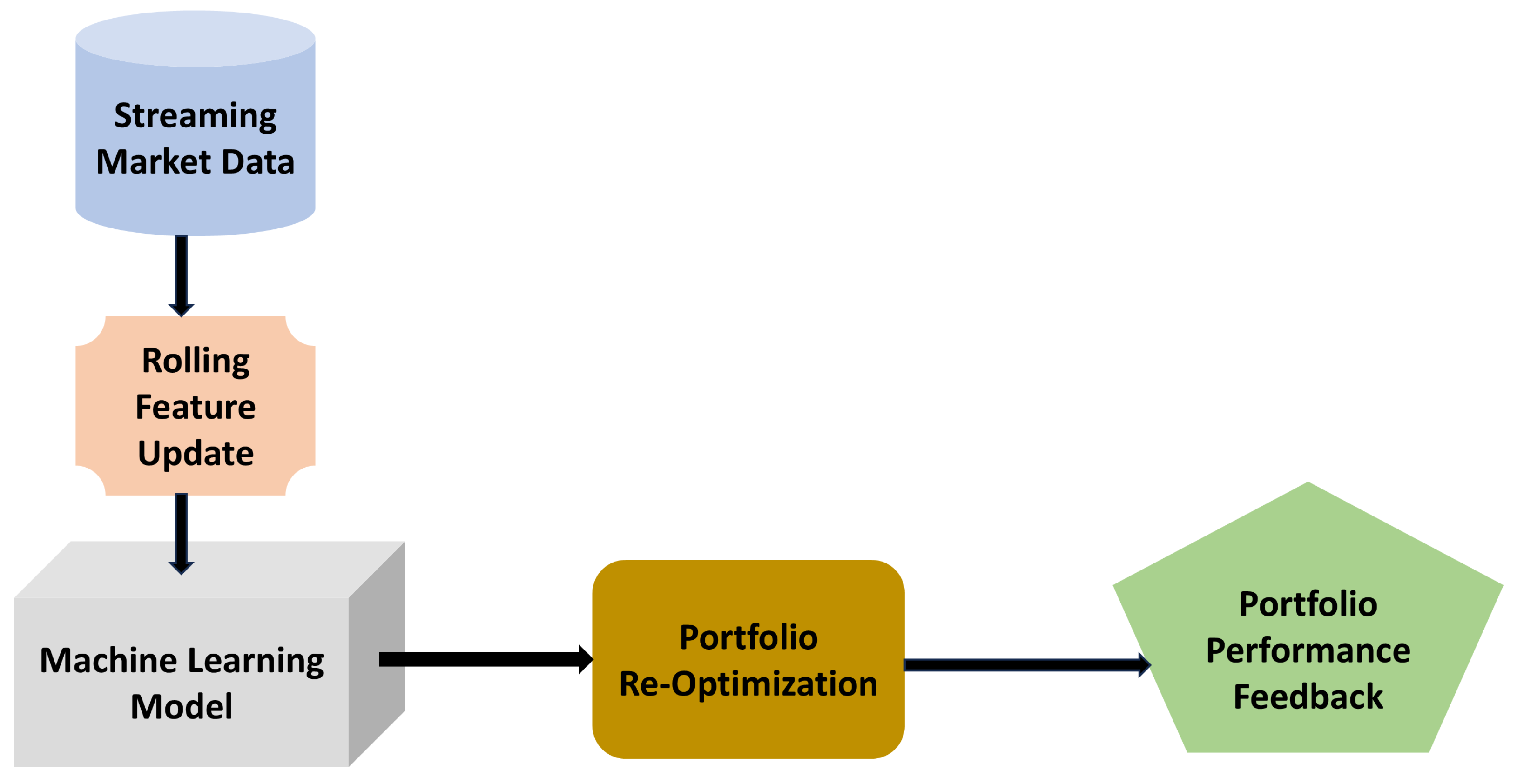Figure 2 illustrates the machine learning-based portfolio optimization framework, where portfolio decisions are updated using rolling historical data and predictive models. Unlike classical approaches, this framework introduces data-driven adaptability. However, it still lacks an explicit mechanism for sequential decision-making and risk-aware policy learning.

These methods frequently convert portfolio optimization to a statistical learning task and use historical data to better estimate the return distribution or risk parameters. Regularization, shrinkage methods, and predictive modeling can help to lower estimation error for high-dimensional asset spaces. As a result, machine learning-based methods achieve improved risk-adjusted performance compared to classically based optimization techniques [21,22].

However, a limitation of most ML-based approaches is their static nature. Portfolios are usually calculated using the historical window, without assuming any form of temporal structure of a decision or feedback of the changing market environment [23]. Thus, the portfolio cannot update well for quick shifts in the financial environment.

Additionally, various heuristic and metaheuristic optimization techniques, including genetic algorithms and particle swarm optimization, have been deployed for building and solving highly complicated constrained portfolio optimization problems but are regarded as black-box optimizers without a theoretical basis and tight integration with stochastic financial models, applied to non-convex objectives and practical constraints [24].

2.3. Reinforcement Learning for Financial Decision-Making

Reinforcement learning is a natural choice for sequential decision-making under uncertainty and has received substantial recent interest from the finance community for algorithmic trading and portfolio management applications [25,26]. By modeling financial decision problems as Markov decision processes, reinforcement learning enables agents to learn adaptive policies directly from interactions with the market [27,28].

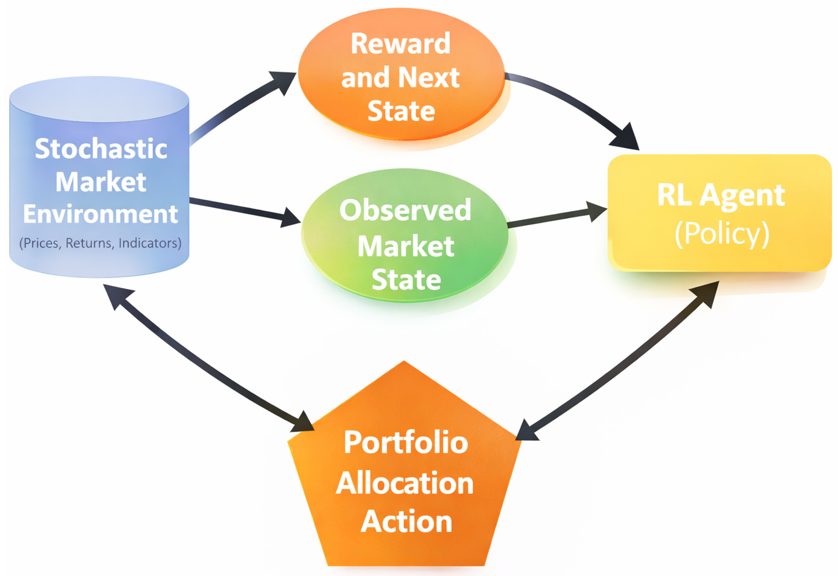
Figure 3 depicts the interaction between the reinforcement learning agent and the financial market environment. The agent observes the market state, selects portfolio allocation actions, and receives feedback in the form of rewards. This iterative process enables continuous learning and adaptation, making reinforcement learning suitable for dynamic portfolio optimization.

Several studies have explored deep RL frameworks for portfolio management and trading strategies [29,30,31,32]. RL may be applied in the framework of portfolio optimization, whereby portfolio allocation decisions are adjusted dynamically as new market data is being received. In contrast to classical and machine learning-based methods, which usually assume the use of static or re-estimated models and models, reinforcement learning encodes the temporal characteristics of financial markets by using state transitions and maximizing returns in the long term. Such a chronologically constructed formulation allows RL to be especially useful in real-time portfolio rebalancing in non-stationary settings [33].

Nonetheless, much of the available RL literature in finance uses risk-neutral reward models that aim to maximize the cumulative returns, which are expected as a result of uncertainty. Though these goals might be high-paying under the right market conditions, they might also promote aggressive investment with a high negative risk in the portfolio when the market is under stress or in times of extreme volatility. Consequently, risk-neutral policies of reinforcement learning can have unstable performance and massive drawdowns [34].

Other recent investigations into risk-conscious and distributional reinforcement learning algorithms have started, but there has been a relative lack of integration between coherent risk measurements and reinforcement learning. Specifically, there are few works that explicitly use risk measures, e.g., Conditional Value-at-Risk, in reinforcement learning objectives and still remain consistent with stochastic market models based on mathematical finance. This void encourages the design of reinforced learning models that mutually deal with sequential decision-making, stochastic market, and principled downside risk regulation.

2.4. Risk-Sensitive Reinforcement Learning

To address the limitations of risk-neutral approaches, recent research has explored risk-sensitive reinforcement learning methods [35] that incorporate risk measures into the learning objective. In particular, CVaR [36,37] has been adopted to explicitly control tail risk in sequential decision-making problems. They introduced a sampling-based method for optimizing CVaR in reinforcement learning problems, which allows controlling tail risk explicitly when optimizing policies. Similarly, Chow et al. [38] came up with risk-constrained reinforcement learning algorithms which use percentile-based risk requirements incorporated into Markov decision processes.

Other studies have investigated alternative downside risk measures, such as maximum drawdown and downside deviation, within reinforcement learning-based portfolio management systems. These approaches aim to improve robustness by penalizing adverse outcomes during training [32].

In spite of all these advances, comparatively few studies have explored reinforcement learning structures involving coherent risk measures, stochastic financial modeling, and actor–critic learning structures, which do not exist under a single portfolio optimization framework [39]. The current paper is an addition to this trend, as it incorporates the risk control using CVaR in a reinforcement learning model based on stochastic market dynamics [40,41].

2.5. Summary and Positioning of the Present Work

Classical portfolio optimization, while theoretically sound, offers poor adaption to changing market conditions. Machine learning-based approaches, while more robust, are static in nature. Reinforcement learning introduces dynamic decision-making, but is formulated without consideration of risk. In this work, we overcome these limitations by proposing a risk-sensitive reinforcement learning-based approach in which market dynamics are modeled using stochastic differential equations and a coherent measure of risk is used to incorporate downside risk directly into the dynamic optimization.

3. Problem Formulation and Stochastic Market Model

3.1. Notation

The different symbols used in this paper are summarized in

Table 1. Notation summary.

Symbol	Description
$S_t^i$	Price of asset i at time t
${\mu }_i$	Expected return of asset i
${\sigma }_i$	Volatility of asset i
$W_t^i$	Brownian motion associated with asset i
${\pi }_t$	Portfolio allocation vector at time t
$V_t$	Portfolio value at time t
$r_t$	Logarithmic portfolio return
$G_T$	Cumulative discounted return
$L_T$	Cumulative loss ($L_T=-G_T$)
$\alpha$	Confidence level for CVaR
$\lambda$	Risk-aversion parameter
$\eta$	Value-at-risk (VaR) threshold
$\gamma$	Discount factor
$\theta$	Policy (actor) parameters
$\varphi$	Value function (critic) parameters

.

3.2. Stochastic Market Model

A continuous-time financial market composed of one risk-free asset and N risky assets is considered. The market dynamics are modeled on a filtered probability space $(\mathsf{\Omega },\mathcal{F},{\left\{{\mathcal{F}}_t\right\}}_{t\ge 0},\mathbb{P})$, which supports a standard N-dimensional Brownian motion ${\mathbf{W}}_t=(W_t^1,\dots ,W_t^N)$ [12,13]. The price process of the i-th risky asset, denoted by $S_t^i$, follows a stochastic differential equation (SDE) of the form

$$d{S}_t^i={\mu }_i{S}_t^{i}dt+{\sigma }_i{S}_t^{i}d{W}_t^i,$$

(1)

where $i=1,\dots ,N$, which corresponds to the geometric Brownian motion model widely used in continuous-time financial modeling [10,12]. Here ${\mu }_i\in \mathbb{R}$ represents the expected return rate and ${\sigma }_i>0$ denotes the volatility of asset i. The Brownian motions may be correlated, with correlation structure

$$\mathbb{E}\left[d{W}_t^{i}d{W}_t^j\right]={\rho }_{ij}dt,$$

(2)

where ${\rho }_{ij}$ denotes the correlation coefficient between assets i and j. The risk-free asset grows deterministically according to

$$d{B}_t=r{B}_{t}dt,$$

(3)

where $r\ge 0$ denotes the constant risk-free interest rate [11].

3.3. Portfolio Dynamics

Let ${\pi }_t=({\pi }_t^1,\dots ,{\pi }_t^N)$ denote the portfolio allocation vector at time t, where ${\pi }_t^i$ represents the proportion of wealth invested in asset i. The portfolio is assumed to be self-financing and satisfies the budget constraint

$$\sum _{i=1}^N{\pi }_t^i=1.$$

(4)

Let $V_t$ denote the portfolio value process. Under the self-financing assumption, the portfolio dynamics are given by

$${\displaystyle \frac{d{V}_t}{V_t}}=\sum _{i=1}^N{\pi }_t^i{\displaystyle \frac{d{S}_t^i}{S_t^i}},$$

(5)

which follows from classical continuous-time portfolio theory [10,13].

The portfolio weights ${\pi }_t$ represent allocations among risky assets, while the remaining fraction of wealth may be invested in the risk-free asset. Under this representation, the wealth dynamics implicitly incorporate the risk-free component through the budget constraint. Substitution of Equation (1) into Equation (5) yields

$$d{V}_t=V_t\left(\sum _{i=1}^N{\pi }_t^i{\mu }_i\right)dt+V_t\sum _{i=1}^N{\pi }_t^i{\sigma }_{i}d{W}_t^i.$$

(6)

3.4. Discrete-Time Approximation

To facilitate the reinforcement learning formulation, the  continuous-time dynamics are discretized over a finite time horizon $[0,T]$ with step size $\Delta t$. Such discretization is commonly used when linking stochastic financial models with data-driven learning frameworks [34]. The discretized portfolio return over one time step can be expressed as

$$R_{t+1}=\sum _{i=1}^N{\pi }_t^i\left({\mu }_i\Delta t+{\sigma }_i\sqrt{\Delta t}{ϵ}_{t+1}^i\right),$$

(7)

where ${\epsilon }_{t+1}^i\sim \mathcal{N}(0,1)$ are standard normal random variables capturing market uncertainty. This discrete-time formulation enables portfolio optimization to be modeled as a sequential decision-making problem in which portfolio weights ${\pi }_t$ are updated dynamically based on observed market states.

Equation (7) provides a discrete approximation of the continuous-time model. However, in practice, the experiments use observed historical asset returns rather than simulated Gaussian noise. In the learning process, realized market returns are used to represent stochastic changes ${\sigma }_i\sqrt{\Delta t}{\epsilon }_{t+1}^i$. Drift and volatility are estimated using a sliding window approach to maintain consistency and avoid look-ahead bias, which is standard in financial modeling [20].

The stochastic differential equation (SDE) framework is used to provide a theoretical description of asset dynamics and to define the reinforcement learning formulation. However, the model is implemented using real historical market data rather than simulated processes. In this framework, the SDE provides structure, while the reinforcement learning agent learns directly from observed data.

3.5. Financial Modeling Assumptions

Under the following assumptions, the proposed market model is developed:

• Markets are assumed to be frictionless, with no transaction costs or taxes.
• Short selling is permitted.
• Asset prices follow continuous stochastic processes driven by Brownian motion.
• Portfolio rebalancing occurs at discrete time intervals.

These assumptions provide the analytical tractability and ease the incorporation with the reinforcement learning techniques. Although the real financial markets are characterized by transaction costs, liquidity limits, and market impact effects, the current formulation acts as a framework of reference in examining a risk-sensitive optimal portfolio under stochastic dynamics. It is possible to add extensions that use transaction costs and other market frictions to the same reinforcement learning structure.

4. Proposed Risk-Sensitive Reinforcement Learning Framework

In this section, the portfolio optimization problem is defined as a risk-sensitive reinforcement learning problem. It is designed to examine an adaptive policy of portfolio allocation that takes into account stochastic market dynamics and which directly makes use of downside risk measures by consistency risk.

4.1. Proposed Framework Overview

This section presents the proposed risk-sensitive reinforcement learning framework for portfolio optimization under stochastic market dynamics. The framework integrates stochastic financial modeling, sequential decision-making, and coherent risk measures into a unified structure. By incorporating CVaR directly into the learning objective and employing an actor–critic architecture, the approach enables adaptive portfolio strategies that balance return maximization with downside risk control. 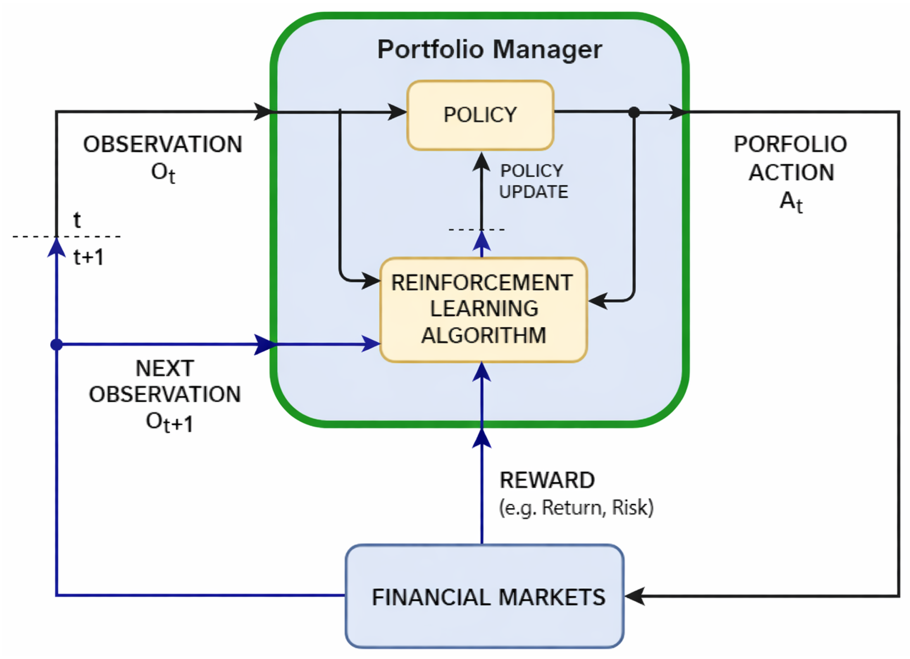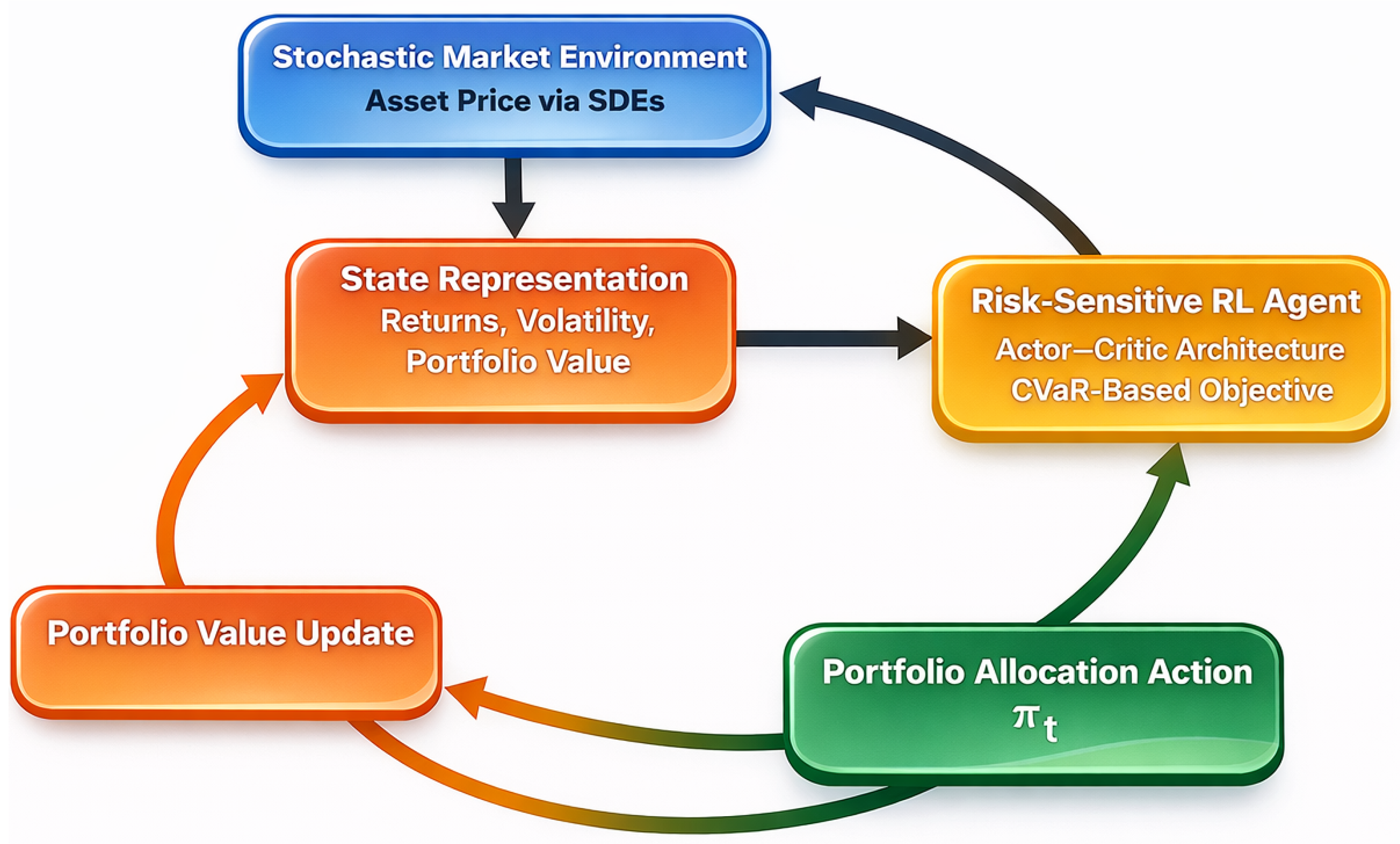Figure 4 illustrates the overall framework of the proposed risk-sensitive reinforcement learning approach for portfolio optimization.

In this framework, the portfolio manager acts as an agent that interacts with financial markets by observing market states and making portfolio allocation decisions. The reinforcement learning algorithm updates the policy based on received rewards, which incorporate both return and risk measures such as CVaR.

4.2. Markov Decision Process Formulation

The portfolio optimization problem is defined as a Markov decision process [42] characterized by the following parameters (defined in reference-chang) as the tuple: $(\mathcal{S},\mathcal{A},\mathcal{P},\mathcal{R},\gamma )$:

• $\mathcal{S}$ is the state space, which is observable information about the market in terms of returns on assets, volatility, and portfolio value.
• $\mathcal{A}$ denotes the action space, where an action corresponds to selecting a portfolio allocation vector ${\pi }_t\in {\mathbb{R}}^N$ satisfying ${\sum }_{i=1}^N{\pi }_t^i=1$.
• $\mathcal{P}$ is the state transition dynamics that are based on the stochastic market model as in Section 3.
• $\mathcal{R}$ denotes the rewarded function.
• $\gamma \in (0,1]$ is the rebate factor.

In each step of decision epoch t, the agent observes the state $s_t\in \mathcal{S}$, selects an action ${\pi }_t\in \mathcal{A}$, and transitions to a new state $s_{t+1}$ according to the market dynamics.

4.3. Risk-Neutral Objective

The objective of reinforcement learning is to maximize the expected cumulative discounted reward,

$$\underset{\pi }{max}\mathbb{E}\left[\sum _{t=0}^T{\gamma }^t{r}_t\right],$$

(8)

where $r_t$ denotes the immediate reward, defined as the portfolio return or log-return at time t. The discount factor $\gamma \in (0,1]$ determines the relative importance of future rewards. From an economic perspective, discounting reflects time preference and uncertainty, as investors typically place greater value on near-term returns compared to distant future outcomes. From a reinforcement learning perspective, the discount factor ensures well-defined cumulative rewards and improves training stability by limiting the influence of long-term uncertainty. When $\gamma =1$, all time periods are treated equally, corresponding to a long-term investment horizon, whereas smaller values of $\gamma$ emphasize short-term performance. Although this formulation would maximize returns, it does not directly manage tail risk, and can lead to policies that are very sensitive to negative market outcomes.

4.4. Risk-Sensitive Objective with Coherent Risk Measures

In order to explicitly model the downside risk in the learning process, CVaR is used. Because CVaR is defined as the losses instead of the gains, we begin by defining the cumulative losses of the investment made on the investment horizon T as follows. To explicitly account for downside risk within the learning process, we incorporate CVaR into the reinforcement learning objective. Since CVaR is defined with respect to losses rather than gains, we first introduce the cumulative portfolio loss over the investment horizon T as

$$L_T=-G_T,$$

(9)

where $G_T$ denotes the cumulative discounted portfolio return. At a confidence level $\alpha \in (0,1)$, the Conditional Value-at-Risk of the loss [43] is defined as

$${\mathrm{CVaR}}_{\alpha }\left(L_T\right)=\underset{\eta \in \mathbb{R}}{min}\left[\eta +{\displaystyle \frac{1}{1-\alpha }}\mathbb{E}\left[{(L_T-\eta )}^{+}\right]\right],$$

(10)

where $\eta \in \mathbb{R}$ represents the Value-at-Risk (VaR) threshold at confidence level $\alpha$, and ${\left(x\right)}^{+}=max(x,0)$.

CVaR is a coherent risk measure, meaning it satisfies the following properties: (i) monotonicity, (ii) subadditivity, (iii) translation invariance, and (iv) positive homogeneity. These properties ensure consistent and rational assessment of financial risk and make CVaR particularly suitable for portfolio optimization under uncertainty. This representation reflects the anticipated amount of excessive losses exceeding the specified confidence level; hence, it offers an a priori account of tail risk. The ensuing risk-sensitive objective functional is provided by

$$J\left(\theta \right)={\mathbb{E}}_{{\pi }_{\theta }}\left[G_T\right]-\lambda {\mathrm{CVaR}}_{\alpha }\left(L_T\right),$$

(11)

where $\lambda \ge 0$ is a risk-aversion parameter that governs the trade-off between return maximization and tail-risk mitigation. Unlike conventional risk-neutral reinforcement learning, in this formulation, the policy is encouraged to optimize the expected returns, as well as to restrict the exposure to large negative events.

4.5. Policy Parameterization and Risk-Sensitive Learning

The portfolio allocation policy is parameterized by $\theta$ and denoted by ${\pi }_{\theta }(a_t\mid s_t)$, where $a_t$ represents the portfolio weight vector selected at state $s_t$. The policy is implemented using a neural network architecture to handle high-dimensional action spaces. To estimate long-term value, a critic network parameterized by $\varphi$ is used to approximate the value function $V_{\varphi }\left(s_t\right)$. The actor–critic structure provides stable learning by combining policy gradient updates with value function approximation.

The risk-sensitive objective is defined as

$$J\left(\theta \right)={\mathbb{E}}_{{\pi }_{\theta }}\left[G_T\right]-\lambda {\mathrm{CVaR}}_{\alpha }\left(L_T\right),$$

(12)

where $L_T=-G_T$ denotes the cumulative portfolio loss, $\lambda \ge 0$ is the risk-aversion parameter, and $\alpha \in (0,1)$ is the confidence level. Using the auxiliary variable formulation of CVaR, we define the joint objective

$$F(\theta ,\eta )={\mathbb{E}}_{{\pi }_{\theta }}\left[G_T\right]-\lambda \left(\eta +{\displaystyle \frac{1}{1-\alpha }}{\mathbb{E}}_{{\pi }_{\theta }}\left[{(L_T-\eta )}^{+}\right]\right),$$

(13)

and consider the optimization problem ${max}_{\theta }{min}_{\eta }F(\theta ,\eta ).$ Using the likelihood ratio identity, the gradient of the expected return term is defined as

$${\nabla }_{\theta }{\mathbb{E}}_{{\pi }_{\theta }}\left[G_T\right]={\mathbb{E}}_{{\pi }_{\theta }}\left[{\nabla }_{\theta }log{\pi }_{\theta }\left(\tau \right)G_T\right],$$

(14)

where $\tau$ denotes a trajectory generated under policy ${\pi }_{\theta }$. Similarly, the gradient of the CVaR term is

$${\nabla }_{\theta }{\mathbb{E}}_{{\pi }_{\theta }}\left[{(L_T-\eta )}^{+}\right]={\mathbb{E}}_{{\pi }_{\theta }}\left[{\nabla }_{\theta }log{\pi }_{\theta }\left(\tau \right){(L_T-\eta )}^{+}\right].$$

(15)

Combining these results yields the gradient of the risk-sensitive objective:

$${\nabla }_{\theta }J\left(\theta \right)={\mathbb{E}}_{{\pi }_{\theta }}\left[{\nabla }_{\theta }log{\pi }_{\theta }\left(\tau \right)\left(G_T-{\displaystyle \frac{\lambda }{1-\alpha }}{(L_T-\eta )}^{+}\right)\right].$$

(16)

This expression demonstrates that the changes in policy due to updated information are affected not by total-return but by large losses that are above the Value-at-Risk level which introduces the tail-risk sensitivity directly into the learning process.

4.6. Actor Loss Function & Critic Update

In practical implementation, the actor is updated by minimizing the surrogate loss

$${\mathcal{L}}_{\mathrm{actor}}=-log{\pi }_{\theta }(a_t\mid s_t)·{\widehat{A}}_t^{\mathrm{risk}},$$

(17)

where the risk-adjusted advantage estimator is defined as

$${\widehat{A}}_t^{\mathrm{risk}}=G_T-{\displaystyle \frac{\lambda }{1-\alpha }}{(L_T-\eta )}^{+}.$$

(18)

The critic network is trained to approximate the value function by minimizing the temporal-difference loss:

$${\mathcal{L}}_{\mathrm{critic}}={\left(r_t+\gamma V_{\varphi }\left(s_{t+1}\right)-V_{\varphi }\left(s_t\right)\right)}^2,$$

(19)

where $\gamma$ denotes the discount factor. The derivative of the CVaR term with respect to $\eta$ is given by

$${\displaystyle \frac{\partial }{\partial \eta }}=1-{\displaystyle \frac{1}{1-\alpha }}{\mathbb{E}}_{{\pi }_{\theta }}\left[{\mathbf{1}}_{\{L_T>\eta \}}\right],$$

(20)

where ${\mathbf{1}}_{\{·\}}$ is the indicator function. Accordingly, the auxiliary variable $\eta$ is updated via gradient descent:

$$\eta \leftarrow \eta -{\beta }_{\eta }\left(1-{\displaystyle \frac{1}{1-\alpha }}\mathbb{E}\left[{\mathbf{1}}_{\{L_T>\eta \}}\right]\right),$$

(21)

where ${\beta }_{\eta }$ is the learning rate for the risk threshold parameter. This joint optimization procedure yields a principled actor–critic implementation of risk-sensitive reinforcement learning with coherent tail-risk control.

Algorithm 1 summarizes the proposed risk-sensitive reinforcement learning procedure for portfolio optimization.

Algorithm 1: Risk-Sensitive Reinforcement Learning for Portfolio Optimization

1: Input: market states $s_t$, risk parameters $\lambda ,\alpha$ 2: Output: learned risk-sensitive portfolio policy ${\pi }_{\theta }$ 3: Initialize policy network parameters $\theta$ and value network parameters $\varphi$ 4: Initialize CVaR auxiliary variable $\eta$ 5: Set risk aversion parameter $\lambda$ and confidence level $\alpha$ 6: for each training episode do 7:     Initialize portfolio value $V_0$ and observe initial state $s_0$ 8:     for $t=0$ to $T-1$ do 9:           Sample portfolio allocation ${\pi }_t\sim {\pi }_{\theta }(·\mid s_t)$ 10:         Execute action ${\pi }_t$ in the stochastic market environment 11:         Observe portfolio return $r_t$ and next state $s_{t+1}$ 12:         Store transition $(s_t,{\pi }_t,r_t,s_{t+1})$ 13:     end for 14:     Compute cumulative return $G_T={\sum }_{t=0}^T{\gamma }^t{r}_t$ 15:     Define cumulative loss $L_T=-G_T$ 16:     Compute risk-adjusted advantage 17:     Compute ${\widehat{A}}^{risk}=G_T-{\displaystyle \frac{\lambda }{1-\alpha }}{(L_T-\eta )}^{+}$ 18:     Estimate policy gradient 19:     Compute $g_{\theta }={\nabla }_{\theta }log{\pi }_{\theta }\left(\tau \right)·{\widehat{A}}^{risk}$ 20:     Update policy parameters $\theta \leftarrow \theta +{\beta }_{\theta }{g}_{\theta }$ 21:     Update value network parameters $\varphi$ using temporal-difference learning 22:     Update CVaR auxiliary variable 23:     Update $\eta \leftarrow \eta -{\beta }_{\eta }\left(1-{\displaystyle \frac{1}{1-\alpha }}{\mathbf{1}}_{\{L_T>\eta \}}\right)$ 24: end for

4.7. Computational Complexity

The computational complexity of the proposed actor–critic reinforcement learning framework can be characterized in terms of the neural network architecture and training horizon. Let N denote the number of assets, d the state dimension, L the number of network layers, H the number of hidden units per layer, and T the length of each training episode. The computational cost of a single forward or backward pass through the network is approximately $O\left(L{H}^2\right)$.

During each training episode of length T, the policy and value networks are updated using gradient-based optimization. Consequently, the overall complexity of a single training episode is approximately $\mathcal{O}(T·L{H}^2)$. If the training process runs for E episodes, the total computational complexity becomes $\mathcal{O}(E·T·L{H}^2)$. In practice, the training process is efficiently parallelizable across trajectories, making the framework scalable to large financial datasets.

Figure 5 shows a schematic diagram of the proposed robust reinforcement learning framework. It highlights that the actor–critic learning maximizes the CVaR for a portfolio of assets, taking into account the stochastic market dynamics. It also emphasizes that the proposed robust reinforcement learning framework utilizes CVaR as objective function for the reinforcement learning framework. It also highlights that the proposed reinforcement framework utilizes the stochastic market dynamics to evaluate the portfolio proceeds.

5. Theoretical Analysis

This section provides the theoretical analysis of the proposed risk-sensitive reinforcement learning framework. While the main tools used in the analysis are stochastical approximation and convex optimization, their application in a CVaR-based reinforcement learning setting leads to new understandings of the learning process and the behaviour of the model. The analysis demonstrates that risk measures can be incorporated into the policy optimization procedure in a unified way, which results in a more stable learning process, while preserving important properties, such as convexity in the auxiliary variable. It also demonstrates convergence of the model to stable solutions.

5.1. Stability of Portfolio Dynamics

Consider the portfolio value process ${\left\{V_t\right\}}_{t=0}^T$ generated by the policy ${\pi }_{\theta }$ in the stochastic market environment. The wealth evolution follows the discrete-time dynamics

$$V_{t+1}=V_t\left(1+{\pi }_t^{\top }{r}_{t+1}\right),$$

(22)

where ${\pi }_t$ denotes the portfolio weight vector and $r_{t+1}$ the asset return vector.

To ensure economic feasibility, we impose the condition that portfolio weights are selected such that the portfolio return satisfies ${\pi }_t^{\top }{r}_{t+1}>-1$ almost surely. This guarantees that the portfolio value remains strictly positive, i.e., $V_{t+1}>0$. In practice, this condition is reasonable, as asset returns are bounded below by $-1$, and portfolio allocation constraints prevent extreme leverage that could result in negative wealth. Under bounded returns and admissible portfolio constraints (e.g., $\parallel {\pi }_t{\parallel }_1\le 1$), the wealth process remains well-defined and finite for all $t\le T$. Consequently, the cumulative return

$$G_T=\sum _{t=0}^T{\gamma }^t{r}_t,$$

(23)

and the corresponding loss $L_T=-G_T$ are well-defined random variables. This ensures that the CVaR-based objective is properly defined within the reinforcement learning framework.

5.2. Assumptions for Theoretical Analysis

To formally analyze the stability and convergence properties of the proposed risk-sensitive reinforcement learning framework, we introduce the following standard assumptions.

Assumption 1

(Bounded Rewards). The portfolio returns $r_t$ are assumed to be bounded, i.e., $|r_t|\le R_{max}<\infty$. It is used in reinforcement learning to ensure stable gradient estimates and convergence. In practice, financial returns may show heavy-tailed behavior. In empirical implementation, the effect of extreme returns is reduced through normalization and the use of finite samples.

Assumption 2

(Smooth Policy Parameterization). The policy ${\pi }_{\theta }\left(a\right|s)$ is continuously differentiated with respect to θ, and the scoring function ${\nabla }_{\theta }log{\pi }_{\theta }\left(a\right|s)$ is bounded.

Assumption 3

(Finite Variance). The cumulative return $G_T$ and cumulative loss $L_T$ have finite second moments under policy ${\pi }_{\theta }$.

These assumptions are standard in policy gradient analysis and ensure that the gradient estimators are well-defined and have finite variance.

5.3. Properties of the Risk-Sensitive Objective

Proposition 1

(Convexity in the Auxiliary Variable). For fixed policy parameters θ, the function $\eta +{\displaystyle \frac{1}{1-\alpha }}\mathbb{E}\left[{(L_T-\eta )}^{+}\right]$ is convex in η.

Proof. 

The function ${\left(x\right)}^{+}=max(x,0)$ is convex. Since expectation preserves convexity, $\mathbb{E}\left[{(L_T-\eta )}^{+}\right]$ is convex in $\eta$. The sum of a linear function in $\eta$ and a convex function is convex, establishing the result. □

Convexity in $\eta$ guarantees that the auxiliary risk threshold admits a well-defined minimizer for fixed policy parameters, ensuring stable risk adjustment during learning. The objective function $F(\theta ,\eta )$ is convex in the auxiliary variable $\eta$ due to the convexity of the CVaR formulation. However, the objective is generally non-convex in the policy parameters $\theta$ because of the nonlinear parameterization of the policy through neural networks. Despite this, the convexity in $\eta$ ensures stable optimization of the risk threshold, while gradient-based methods are used to obtain locally optimal solutions in $\theta$.

Under standard assumptions of bounded rewards and compact parameter spaces, the objective function $F(\theta ,\eta )$ is well-defined and admits at least one stationary solution. In particular, the convexity in $\eta$ guarantees the existence of an optimal risk threshold for a fixed policy, while the policy optimization seeks locally optimal solutions in the parameter space.

5.4. Convergence Properties

Under Assumptions 1–3, the gradient estimator of the risk-sensitive objective

$${\nabla }_{\theta }J\left(\theta \right)={\mathbb{E}}_{{\pi }_{\theta }}\left[{\nabla }_{\theta }log{\pi }_{\theta }\left(\tau \right)\left(G_T-{\displaystyle \frac{\lambda }{1-\alpha }}{(L_T-\eta )}^{+}\right)\right],$$

(24)

is well-defined and has finite variance. The convergence result relies on standard stochastic approximation conditions, including diminishing step sizes satisfying ${\sum }_{k=1}^{\infty }{\beta }_k=\infty$ and ${\sum }_{k=1}^{\infty }{\beta }_k^2<\infty$, boundedness of gradients, and finite variance of the stochastic updates.

Proposition 2

(Local Convergence of Risk-Sensitive Policy Gradient). Suppose the learning rates $\left\{{\beta }_{\theta }\right\}$ and $\left\{{\beta }_{\eta }\right\}$ satisfy the standard stochastic approximation conditions:

$$\sum _{k=1}^{\infty }{\beta }_k=\infty ,\sum _{k=1}^{\infty }{\beta }_k^2<\infty .$$

Then, under Assumptions 1–3, the joint updates of $(\theta ,\eta )$ converge almost surely to a stationary point of the risk-sensitive objective $F(\theta ,\eta )$, in the sense of stochastic approximation theory.

Proof. 

The objective $F(\theta ,\eta )$ is continuously differentiable in $\theta$ under Assumption 2 and convex in $\eta$ by Proposition 1. Under bounded rewards and finite variance (Assumptions 1 and 3), the gradient estimators satisfy standard martingale difference noise conditions. Therefore, the convergence follows from classical stochastic approximation theory for policy gradient methods. □

Although a complete formal proof is beyond the scope of this paper, the convergence follows from classical results in stochastic approximation and policy gradient methods, under the stated assumptions. The proof sketch provided outlines the key arguments supporting convergence.

6. Experimental Setup and Results

This section presents the datasets, benchmark methods, evaluation metrics, and implementation details used to assess the proposed risk-sensitive reinforcement learning framework. The evaluation focuses on out-of-sample performance and compares the proposed approach with both classical and learning-based benchmark methods. Performance is measured across rolling test windows, and final results are reported as averages over 12–14 out-of-sample evaluation periods to ensure robustness.

6.1. Experimental Setup

The empirical study is conducted using daily closing price data of stocks from the NIFTY 50 index (National Stock Exchange, India) over the period January 2015 to December 2025. The dataset captures different market regimes, including stable periods, high volatility phases, and the COVID-19 market crash, making it suitable for evaluating model robustness. Data are collected from publicly available sources such as the NSE database, Yahoo Finance, and Rediff Money.

Logarithmic returns are used to calculate daily returns, where the value of logarithmic returns is computed as $r_t=log(P_t/P_{t-1})$, where $P_t$ is the closing price at time t. The reason that log returns are used is that they are numerically stable and additive with time. It is important for learning to be consistent that the training data has all the features normalized. Rolling returns and volatility should be multiplied by the mean and standard deviation respectively. This will help to avoid leakage of information and to standardize the training and test setting. The dataset contains some worst market situations, in particular, those during the COVID-19 crash, that are an important benchmark for downside risk management. In such situations, the proposed framework is more stable and less prone to drawdowns compared to the baselines, hence demonstrating the importance of the CVaR term in the learning objective.

In order to investigate the distributional characteristics of asset returns, we calculate the descriptive statistics of the mean, standard deviation, skewness, and kurtosis for each selected assets. The results indicate that the asset return is characterized by the negative skewness and excess kurtosis, or the asymmetric and heavy-tailed distribution, which is typical in financial markets. However, to support these findings we use the Jarque–Bera test to test for normality. The test rejects the null hypothesis of a normal distribution at the normal levels of significance and so demonstrates that asset returns are not Gaussian. These findings justify the use of CVaR as a risk measure as it is specifically designed to reflect tail risk and extreme losses which are not captured well by variance-based measures.

The results indicate negative skewness and high kurtosis for asset returns. This implies that the distributions are asymmetric and have heavy tails. This is the typical behaviour of financial markets. The Jarque–Bera test similarly rejects normality at 5%; the results provide strong evidence against this hypothesis. In addition to CVaR and maximum drawdown, it is possible to explore the distributional properties of a risk (skewness and kurtosis), which would provide more insight into risk. These characteristics, as can be seen in

Table 2. Descriptive statistics of asset returns.

Asset	Mean	Std Dev	Skewness	Kurtosis
Reliance	0.0007	0.0185	−0.48	4.25
HDFC Bank	0.0006	0.0172	−0.42	4.10
ICICI Bank	0.0008	0.0201	−0.55	4.60
Infosys	0.0005	0.0160	−0.35	3.95
TCS	0.0005	0.0153	−0.30	3.85
SBI	0.0007	0.0225	−0.60	4.80
Bharti Airtel	0.0006	0.0180	−0.40	4.05
ITC	0.0004	0.0145	−0.25	3.70
L&T	0.0006	0.0192	−0.45	4.30
Axis Bank	0.0007	0.0210	−0.52	4.55

, are very evident in the data and are common in the real financial time series. This kind of behavior is an indicator of extreme events and non-Gaussian dynamics. Variance-based measures do not adequately explain these effects. Despite the fact that CVaR is used to respond to tail risk, a more specific study of extreme outcomes may further reinforce the risk assessment. This is a significant research field for the future. Trading costs can affect performance in reality because the reinforcement method can assume periodic changes in the portfolio. However, the main objective of the research is to assess the efficiency of the risk-sensitive learning under the conditions of a controlled environment. An extension that will be significant in future work will be the incorporation of transaction costs and other market frictions.

Rolling window is incorporated to test the model in a realistic and time-consistent fashion. This is done through a 3-year training period (with trading of about 750 trading days) and a 6-month testing period (with trading of about 125 trading days). A dataset is then reduced by shifting the window with the aim of creating a combination of various train–test splits. In such a way, the model is trained at all times using the historic data, and its assessment is carried out on a set of future data. To reduce overfitting, the model is retrained for each rolling window, and results are averaged across all evaluation periods. Multiple random seeds are used to account for the stochasticity in reinforcement learning, and the reported results include both the mean and standard deviation to ensure reliability. The state vector at time t includes past-20-day rolling returns for each asset, 20-day rolling volatility estimates computed as standard deviation, and the current portfolio allocation weights. All features are normalized using statistics computed exclusively within the training window to prevent information leakage.

6.2. Implementation Details

The proposed model is implemented in Python using PyTorch for neural network training. NumPy and Pandas are used for data processing and analysis. All experiments are conducted on a standard workstation with an Intel Core i7 processor and 16 GB RAM. The training process is efficient. Each training episode takes about 1–2 s. The complete rolling window backtesting procedure is completed in approximately 2–3 h. This indicates that the framework is computationally feasible for practical applications.

The reinforcement learning agent follows an actor–critic architecture. The actor network consists of two fully connected layers with 128 and 64 neurons, using ReLU activation. The output layer applies a Softmax function to ensure that the portfolio weights sum to one. The critic network has a similar structure but does not use Softmax. Training is performed using the Adam optimizer with a learning rate of ${\beta }_{\theta }=3\times {10}^{-4}$ and a batch size of 64. Each rolling window is trained for 500 episodes. The discount factor is set to $\gamma =0.99$. The CVaR confidence level is fixed at $\alpha =0.95$. The risk-aversion parameter $\lambda$ is selected through validation within the training window.

Performance estimation is carried out for each out-of-sample period and then averaged across all windows to get a general performance measure. The experiments are carried out on NIFTY 50 index data. But the proposed framework is not limited to a particular market or asset class. It is obviously easy to extend it to equities, multi-asset portfolios, commodities and crypto because it is based on fundamental features like return and volatility that are the same across all financial markets.

6.3. Results

The performance of the proposed risk-sensitive reinforcement learning approach is compared against a set of baselines including the Equal-Weight Portfolio, which refers to the simplistic strategy of allocating equal weights to all assets in the portfolio. Mean–Variance Optimization refers to the classic Markowitz mean–variance optimization and is performed using expected returns and covariances. CVaR-Based Optimization refers to the approach of directly optimizing a variant of CVaR which is easier to compute, to be more specific, the Conditional Value-at-Risk or the expected tail-loss. And Risk-Neutral Reinforcement Learning refers to the approach of directly maximizing risk-neutral returns through reinforcement learning. Performance evaluation is conducted using both return-based and risk-adjusted metrics, including Average Return to measure overall profitability, Volatility to assess variability in returns, the Sharpe Ratio to evaluate risk-adjusted performance, Conditional Value-at-Risk (CVaR) to quantify extreme downside risk, and Maximum Drawdown to capture the largest observed loss from peak to trough. Together, these metrics offer a comprehensive assessment of profitability, stability, and exposure to downside risk.

Table 3. Out-of-sample performance comparison of portfolio strategies (mean ± standard deviation).

Method	Return	Volatility	Sharpe	CVaR0.95	Max Drawdown
Equal-Weight	0.072 ± 0.011	0.165 ± 0.012	0.440 ± 0.050	−0.182 ± 0.014	−0.285 ± 0.018
Mean-Variance	0.081 ± 0.013	0.172 ± 0.015	0.470 ± 0.060	−0.176 ± 0.013	−0.268 ± 0.017
CVaR-Based	0.078 ± 0.012	0.158 ± 0.011	0.490 ± 0.050	−0.149 ± 0.010	−0.241 ± 0.015
Risk-Neutral RL	0.094 ± 0.021	0.203 ± 0.019	0.460 ± 0.080	−0.214 ± 0.023	−0.312 ± 0.022
Risk-Sensitive RL (Proposed)	0.089 ± 0.014	0.147 ± 0.010	0.610 ± 0.070	−0.121 ± 0.009	−0.198 ± 0.014

reports the mean and standard deviation of portfolio performance metrics across rolling test windows.

The results show that the risk-neutral RL agent achieves a marginally higher average return, but at the expense of increased volatility and tail risk. The RSRL framework introduced here achieves the best Sharpe for all rolling windows and consistently improves CVaR and max drawdown. This suggests that the inclusion of the tail-risk control improves the risk-adjusted performance without a significant penalty in returns. Also, the mean and standard deviation are calculated over multiple independent runs with different seeds. This ensures that the results are not unreliable due to randomness in the reinforcement learning. To further evaluate the reliability of the observed improvements, paired t-tests are conducted between the proposed RSRL model and baseline methods over rolling test windows. The results confirm that the improvements in Sharpe ratio and CVaR are statistically significant at the 5% significance level (p < 0.05), indicating that the performance gains are not due to random variation.

6.4. Statistical Validation Across Rolling Windows

In order to compare robustness, the paired t-tests will be applied to Sharpe ratios calculated in parallel across identical rolling test windows between the RSRL model and risk-neutral reinforcement learning baseline. The null hypothesis is that the mean difference in the Sharpe ratios at different rolling windows is zero.

The paired t-test yields: $t=2.84,p=0.015$. Since $p<0.05$, the increase in Sharpe ratio as a result of the RSRL framework is statistically significant at the 5% level since p = 0.05. These findings show that the recorded performance improvements are not due to specific market periods but can be maintained at all times even when considering a window of evaluation.

The explicit use of CVaR as a part of the reinforcement learning objective leads to the controlled mitigation of extreme losses. Over rolling evaluation windows, RSRL strategy has lower CVaR_0.95 and lower maximum drawdown than risk-neutral reinforcement learning and classical optimization strategies. This behavior is an indication of the quality of coherent risk regularization that moderates exposure in adverse market conditions.

6.5. Sensitivity Analysis and Robustness

The influence of the risk-aversion parameter $\lambda$ is tested by sweeping across its admissible values. Stronger $\lambda$ lower the portfolio’s volatility and tail risk, but also reduce the average return mildly. This confirms the ability of our framework to flexibly tune the risk–return trade-off according to the preferences of the risk-averse investors. The sensitivity of the model to the CVaR confidence level $\alpha \in \{0.90,0.95,0.99\}$ is also examined. Higher values of $\alpha$ result in more conservative portfolio allocations. This reduces exposure to extreme losses, which is consistent with the role of CVaR in managing tail risk.

The impact of different learning rates $\{{10}^{-3},5\times {10}^{-4},{10}^{-4}\}$ is also analyzed. The model remains stable in this range. Medium learning rates achieve a compromise between speed of convergence and performance. To address the stochasticity inherent in reinforcement learning, we repeated experiments with different random seeds. The reported results are averaged across runs, ensuring robustness and reproducibility.

7. Conclusions and Future Work

This study presents a risk-sensitive reinforcement learning framework for portfolio optimization under stochastic market dynamics. It combines stochastic financial modeling, actor–critic learning, and coherent risk measures in a unified setting. By incorporating Conditional Value-at-Risk (CVaR) into the learning objective, the framework directly controls extreme downside risk while maintaining competitive returns. The empirical results show that the proposed framework outperforms classical portfolio optimization methods and risk-neutral reinforcement learning approaches in terms of risk-adjusted performance. Improvements in the Sharpe ratio, along with reductions in CVaR and maximum drawdown, demonstrate its effectiveness in managing tail risk. This advantage is more evident during volatile market conditions, where traditional methods often become unstable and more exposed to large losses.

From a modeling perspective, stochastic differential equation (SDE)-based dynamics provide a realistic representation of asset behavior. At the same time, reinforcement learning enables adaptive and sequential decision-making in non-stationary environments. This combination allows the model to adjust portfolio allocations dynamically as market conditions change, overcoming the limitations of static approaches. The theoretical analysis supports the validity of the framework. The convexity of the CVaR formulation in the auxiliary variable ensures stable optimization. Convergence under standard assumptions further strengthens the reliability of the method. Although the policy optimization is non-convex due to neural networks, the actor–critic structure allows efficient gradient-based learning.

Despite these strengths, some limitations remain. The model assumes a frictionless market without transaction costs, liquidity constraints, or market impact. This may limit real-world applicability. In addition, the current formulation focuses on terminal risk and does not capture path-dependent or time-consistent risk measures. Future work can extend this framework in several directions. Incorporating transaction costs and liquidity constraints would improve practical relevance. Including path-dependent and time-consistent risk measures could provide better risk control. Exploring advanced reinforcement learning models, such as distributional or transformer-based approaches, may further enhance performance. Evaluating the model across different markets and conducting sensitivity analysis would also improve generalizability.