Subsampling-Based Consensus Hierarchical Clustering for Robust Customer Segmentation with Mixed-Type Data

Abstract

Hierarchical clustering is an unsupervised framework that organizes observations according to pairwise similarity relationships. In this study, an agglomerative hierarchical approach combined with Gower dissimilarity is employed to accommodate mixed-type customer data. To address data quality issues such as missing values and outliers, Multiple Imputation by Chained Equations (MICE) and Winsorization are incorporated into the preprocessing pipeline. To validate cluster stability and identify the optimal number of clusters, we employ silhouette analysis, the Davies–Bouldin Index (DBI), the Proportion of Ambiguous Clustering (PAC), and a subsampling-based consensus clustering framework. A consensus-based hierarchical tree derived from the consensus matrix is employed to assess the robustness of the segmentation structure. The resulting clusters are further evaluated through comparisons with baseline algorithms for mixed-type data, including Partitioning Around Medoids (PAM) based on Gower dissimilarity and the K-prototypes method, together with statistical tests confirming significant behavioral differences between the identified segments. From an application standpoint, these results provide a data-driven basis for customer targeting by identifying distinct behavioral patterns, thereby supporting more effective engagement strategies and optimized resource allocation.

1. Introduction

Consensus clustering aggregates the outcomes of repeated clustering analyses, often based on resampling strategies, to obtain a unified and more stable clustering solution [1,2]. Such an approach becomes especially valuable when dealing with heterogeneous or structurally complex datasets. Results obtained from hierarchical clustering are not always stable, as they may be affected by sampling fluctuations, the choice of distance metrics (e.g., Euclidean or Gower), or small variations in the data [3,4]. Such factors may complicate the interpretation of the resulting clusters. The consensus framework mitigates discrepancies between individual clustering results by focusing on structures that consistently emerge across repeated clustering procedures. This challenge is especially pronounced in mixed-type datasets, where heterogeneous variable types complicate similarity measurement and may affect the stability of the resulting clusters [5,6].

The objective of customer segmentation is to partition a diverse customer base into relatively homogeneous groups using variables such as demographic profiles, psychographic factors, and consumption patterns [7]. Within this framework, consensus trees offer a robust approach for identifying stable customer groups while reducing sensitivity to sampling variability and parameter settings. The identified clusters can provide a more reliable basis for data-driven marketing decisions. From a practical perspective, robust segmentation is critical in marketing analytics because unstable clustering structures may negatively affect targeting strategies and resource allocation.

In the literature, consensus methods are usually grouped into two principal categories: probabilistic and non-probabilistic approaches. Probabilistic consensus methods assume that the observed hierarchies arise from an underlying stochastic process, and the consensus structure is obtained through parameter estimation techniques such as Bayesian inference or mixture modeling [8,9].

By contrast, non-probabilistic methods obtain consensus structures through deterministic rules, including strict consensus and majority-rule consensus, without assuming a probabilistic data-generating process [10].

2. Materials and Methods

2.1. Notation and Some Basic Concepts

In the Section 2.1, we introduce the notation and fundamental definitions adopted throughout the study.

$N, J, K$: denote the numbers of individuals, variables, and clusters, respectively;

• $I=\{1,2,\dots ,N\}$: index set of individuals;
• $X=\left[x_{ij}\right]\in {\mathbb{R}}^{N\times J}$: observed data matrix;
• $\delta =\left[{\delta }_{ij}\right]$: pairwise dissimilarity matrix.

Definition 1.

A dissimilarity matrix, denoted by $\delta =\left[{\delta }_{ij}\right]$ for $i,j\in I$, is a symmetric square matrix of size $N\times N$ that encodes the pairwise dissimilarity between observations in a dataset. Each entry is non-negative, i.e., ${\delta }_{ij}\ge 0$, and the diagonal elements are zero, such that ${\delta }_{ii}=0$ for all i [11].

Definition 2.

A distance matrix is a particular case of a dissimilarity matrix in which the entries correspond to geometric distances between observations. It is a symmetric matrix, i.e., $d_{ij}=d_{ji}$, with non-negative elements $(d_{ij}\ge 0)$ and zero diagonal entries $(d_{ii}=0)$. In addition, it satisfies the triangle inequality, meaning that $d_{ij}\le d_{ik}+d_{kj}$ for all $i,j,k$ [11].

Definition 3.

A consensus matrix, denoted by $M=\left[m_{ij}\right]$ for $i,j\in I$, is a symmetric matrix of size $N\times N$ whose entries lie within the interval $[0,1]$. The diagonal elements are equal to one, i.e., $m_{ii}=1$, while each off-diagonal element $m_{ij}$ quantifies how frequently individuals i and j are assigned to the same cluster over repeated resampling iterations [12].

The following example illustrates how the consensus matrix is constructed. Consider a simple case with $N=5$ individuals and $R=4$ subsampling iterations. Suppose the cluster assignments are:

Iteration 1: $\{1,2\}$ and $\{3,4,5\}$;

Iteration 2: $\{1,2,3\}$ and $\{4,5\}$;

Iteration 3: $\{1,3\}$ and $\{2,4,5\}$;

Iteration 4: $\{1,2\}$ and $\{3,4,5\}$.

The consensus value $m_{ij}$ indicates how often individuals i and j are grouped within the same cluster across different iterations. For example, individuals 1 and 2 appear together in three out of four iterations, giving $m_{12}=3/4=0.75$, whereas individuals 1 and 4 never appear in the same cluster, yielding $m_{14}=0$.

The resulting consensus matrix is

$$M=\left[\begin{array}{ccccc}1& 0.75& 0.50& 0& 0\\ 0.75& 1& 0.25& 0.25& 0.25\\ 0.50& 0.25& 1& 0.50& 0.50\\ 0& 0.25& 0.50& 1& 1\\ 0& 0.25& 0.50& 1& 1\end{array}\right].$$

Definition 4.

Consider two observations $x_i=(x_{i1},x_{i2},\dots ,x_{ip})$ and $x_j=(x_{j1},x_{j2},\dots ,x_{jp})$, each characterized by p variables that can belong to different data types. The Gower similarity coefficient between $x_i$ and $x_j$, denoted by $S_{ij}$, is given by

$$S_{ij}={\displaystyle \frac{{\sum }_{k=1}^p{w}_{ijk}{s}_{ijk}}{{\sum }_{k=1}^p{w}_{ijk}}},$$

where $s_{ijk}$ measures the similarity between $x_i$ and $x_j$ with respect to the k-th variable, and $w_{ijk}\in \{0,1\}$ indicates whether that variable is valid and non-missing for both observations.

The associated Gower dissimilarity [6] is then defined as

$${\delta }_{ij}=1-S_{ij}.$$

2.2. Some Methods of Clustering

Cluster analysis seeks to partition observations into groups according to their degree of similarity. The objective is to obtain clusters in which members of the same group are closely related, whereas elements from different groups are distinctly separated. Most clustering methods are based on distance or similarity metrics, typically combined with criteria that encourage intra-cluster compactness and inter-cluster separation.

Clustering approaches can be broadly divided into five main categories.

1.

Hierarchical Clustering

Hierarchical clustering [13] arranges observations into a nested structure, typically visualized as a dendrogram, which illustrates the relationships among clusters at different levels [14]. Hierarchical clustering procedures are generally divided into agglomerative methods, which iteratively merge clusters, and divisive methods, which recursively partition them [15].

2.

Partition-Based Clustering

Partitioning methods aim to split a finite dataset $X=\{x_1,x_2,\dots ,x_n\}\subset {\mathbb{R}}^m$ into K mutually exclusive and non-empty subsets $C=\{C_1,C_2,\dots ,C_K\}$, where each $C_i\subset X$ [16,17]. The number of clusters K can either be specified in advance or inferred from the underlying data structure.

Most methods in this category can be expressed as the optimization of a global objective function:

$$\mathcal{L}(C,\left\{{\mu }_i\right\})=\sum _{i=1}^K\sum _{x_j\in C_i}\ell (x_j,{\mu }_i),$$

(1)

where ${\mu }_i\in {\mathbb{R}}^m$ represents the prototype (cluster center) associated with cluster $C_i$, and $\ell :{\mathbb{R}}^m\times {\mathbb{R}}^m\to [0,\infty )$ denotes a suitable loss function. Typical examples of partition-based methods include K-means, K-medians, K-modes, and K-medoids.

K-means. The K-means algorithm [18] partitions the dataset into K clusters by repeatedly assigning each observation to its nearest centroid. It seeks to minimize the within-cluster sum of squared distances (WCSS) [19].

$${\mathcal{L}}_{\mathrm{K}-\mathrm{means}}=\sum _{i=1}^K\sum _{x_j\in C_i}{\parallel x_j-{\mu }_i\parallel }_2^2,$$

(2)

K-medians. The K-medians method [20] replaces the mean with the geometric median [21] and minimizes the sum of ${\ell }_1$ distances:

$${\mathcal{L}}_{\mathrm{K}-\mathrm{means}}=\sum _{i=1}^K\sum _{x_j\in C_i}{\parallel x_j-{\mu }_i\parallel }_1,$$

(3)

This formulation provides increased robustness to outliers [22].

K-modes. The K-modes algorithm [23] adapts the K-means approach to categorical data by substituting cluster means with modes and employing appropriate dissimilarity measures, such as the Hamming distance [24].

K-medoids. The K-medoids algorithm [25] characterizes each cluster using a representative observation, referred to as a medoid, and aims to reduce the overall dissimilarity between data points and their closest medoid [26]. This method is particularly useful when Euclidean distance assumptions are not suitable.

Partitioning Around Medoids (PAM). Partitioning Around Medoids (PAM) [25] is a widely used approach for solving the K-medoids clustering problem.

In contrast to centroid-based methods such as K-means, PAM determines cluster centers using actual observations (medoids).

Starting from a dissimilarity matrix $\delta =\left({\delta }_{ij}\right)$, the objective is to identify a set of K medoids $\{m_1,\dots ,m_K\}$ that minimizes the total dissimilarity between each observation and its nearest medoid:

$${\mathcal{L}}_{PAM}=\sum _{i=1}^n\underset{k\in \{1,\dots ,K\}}{min}\delta (x_i,m_k).$$

(4)

The medoids are iteratively refined by exchanging candidate points with current medoids whenever such swaps decrease the objective function. Because PAM relies solely on pairwise dissimilarities rather than Euclidean structure, it can be naturally extended to mixed-type data using measures such as the Gower coefficient.

K-prototypes. The K-prototypes algorithm [27] is designed for clustering data that include both numerical and categorical variables, combining ideas from K-means and K-modes. It uses Euclidean distance for numerical variables and a matching-based dissimilarity for categorical ones.

Let $x_i=(x_i^{\left(num\right)},x_i^{\left(cat\right)})$ denote the numeric and categorical components of observation i. The clustering objective is defined as

$${\mathcal{L}}_{\mathrm{K}-\mathrm{means}}=\sum _{i=1}^n\sum _{k=1}^K{z}_{ik}\left(\parallel x_i^{\left(num\right)}-{\mu }_k^{\left(num\right)}{\parallel }_2^2+\gamma {\delta }_{ik}^{\left(cat\right)}\right),$$

(5)

where $z_{ik}$ is the cluster assignment indicator, ${\mu }_k$ denotes the prototype of cluster k, ${\delta }_{ik}^{\left(cat\right)}$ measures categorical mismatches, and $\gamma$ is a weighting parameter controlling the relative influence of categorical attributes.

This hybrid distance formulation allows K-prototypes to handle mixed-type datasets efficiently while maintaining a partition-based clustering structure.

In this study, PAM and K-prototypes were employed as baseline partitioning algorithms to evaluate the clustering structure produced by the proposed hierarchical consensus framework.

3.

Density-Based Clustering

Density-based clustering characterizes clusters as regions of high data concentration, while areas with low density are treated as noise [28].

The DBSCAN algorithm [29] can identify clusters of arbitrary shape without requiring the number of clusters to be specified in advance [30].

4.

Model-Based Clustering

Model-based clustering formulates the clustering task as fitting a finite mixture of probabilistic distributions to the observed data [31].

Formally, the data distribution can be written as

$$p\left(x\right|\mathrm{\Theta })=\sum _{k=1}^K{\pi }_k{f}_k\left(x\right|{\theta }_k),$$

(6)

where ${\pi }_k$ denotes the mixing weight of component k (${\sum }_{k=1}^K{\pi }_k=1$), $f_k\left(x\right|{\theta }_k)$ corresponds to the density associated with the k-th component, and $\mathrm{\Theta }$ represents the set of model parameters [32].

Cluster assignments are derived from posterior probabilities $P(z_i=k\mid x_i,\mathrm{\Theta })$ obtained via Bayes’ theorem. Model parameters are commonly estimated using the Expectation–Maximization (EM) algorithm [33].

5.

Uncertainty-Based Clustering (Neutrosophic Clustering)

Uncertainty-based clustering generalizes fuzzy clustering by explicitly incorporating indeterminacy into the representation of data. In the neutrosophic framework, each observation is described by a triplet $(T,I,F)$, which quantifies the degrees of truth-membership, indeterminacy, and falsity, respectively [34].

Consider a dataset $X=\{x_1,x_2,\dots ,x_N\}\subset {\mathbb{R}}^d$ comprising N observations, and assume the presence of K clusters with corresponding centroids $C_1,\dots ,C_K$.

For a given observation $x_i$, its neutrosophic representation is defined through three components:

• $T_i\in [0,1]$ quantifies the degree of membership of $x_i$;
• $I_i\in [0,1]$ captures the level of indeterminacy;
• $F_i\in [0,1]$ measures the degree of non-membership (falsity).

Subject to

$$0\le T_i+I_i+F_i\le 3.$$

(7)

The components of the neutrosophic triplet are computed using distance-based formulations commonly adopted in neutrosophic clustering models [35,36]. In the classical neutrosophic framework, the triplet is defined for each observation as $(T_i,I_i,F_i)$.

The truth-membership degree $T_i$ is defined as

$$T_i=\underset{k}{max}\left\{{\displaystyle \frac{1}{{\sum }_{j=1}^K{\left(\frac{d_{ik}}{d_{ij}}\right)}^{\frac{2}{r-1}}}}\right\},$$

(8)

where $d_{ik}$ denotes the distance between observation $x_i$ and cluster centroid $C_k$, and $r>1$ is the fuzzification parameter.

The indeterminacy term $I_i$ reflects the uncertainty in assigning $x_i$ to a particular cluster and is derived from the relative distances to its two closest cluster centers:

$$I_i={\displaystyle \frac{d_{i\left(1\right)}}{d_{i\left(1\right)}+d_{i\left(2\right)}}},$$

(9)

where $d_{i\left(1\right)}$ and $d_{i\left(2\right)}$ denote the distances to the closest and second-closest cluster centroids, respectively. Larger values of $I_i$ indicate observations located near cluster boundaries.

The falsity component represents the degree of non-membership and is defined independently as

$$F_i={\displaystyle \frac{{\sum }_{k=1}^K{d}_{ik}^2}{{\sum }_{k=1}^K{d}_{ik}^2+ϵ}},$$

(10)

where $ϵ>0$ is a small constant to avoid numerical instability. This formulation ensures that $F_i$ is not directly dependent on $T_i$, in accordance with the classical neutrosophic framework.

The corresponding objective function is defined as

$$Q=\sum _{i=1}^N\sum _{k=1}^K{T}_i^r{d}_{ik}^2+\lambda \sum _{i=1}^N{I}_i,$$

(11)

where $d_{ik}$ corresponds to the distance between $x_i$ and centroid $C_k$, $r>1$ determines the degree of fuzziness, and $\lambda$ acts as a regularization term [35].

Cluster centers are updated as

$$C_k={\displaystyle \frac{{\sum }_{i=1}^N{T}_i^r{x}_i}{{\sum }_{i=1}^N{T}_i^r}}.$$

(12)

Neutrosophic clustering has shown strong performance in applications such as image segmentation [37] and medical diagnosis [38], particularly in noisy or uncertain environments due to its explicit modeling of indeterminacy.

Within the context of consensus clustering, the neutrosophic triplet $(T,I,F)$ can be naturally related to the consensus matrix used in the present study. Let $C_{ij}\in [0,1]$ denote the classical consensus value representing the proportion of resampling runs in which observations i and j are clustered together. A neutrosophic representation of this relationship can be expressed as $T_{ij}=C_{ij}$ (stable co-clustering), $F_{ij}=1-C_{ij}$ (separation), and an indeterminacy component $I_{ij}$ that captures ambiguous assignments, which are typically observed when $C_{ij}$ takes intermediate values.

For example, if two observations are clustered together in $90\%$ of the resampling runs ($C_{ij}=0.90$), the pair shows strong stability with low ambiguity. In contrast, a value close to 0.5 indicates high indeterminacy and suggests that the pair lies near a cluster boundary. In a hierarchical framework, such indeterminacy information could be used to identify unstable branches or guide pruning decisions in the consensus tree.

2.3. Methods of Analysis

2.3.1. Hierarchical Clustering

Hierarchical clustering is generally approached through either an agglomerative or a divisive scheme. In the agglomerative case, the procedure starts with each observation forming its own cluster and proceeds by successively combining clusters based on their proximity. At each stage, the closest pair of clusters is merged according to a chosen linkage rule, which defines how inter-cluster distances or similarities are computed.

Under the single linkage criterion, the distance between two clusters is determined by the smallest distance between any two observations belonging to different clusters. Consequently, clusters are merged whenever a pair of observations (each from a different cluster) exhibits the minimum separation.

Let $C=\{C_1,C_2,\dots ,C_K\}$ denote a collection of K clusters, where $n_{C_i}$ represents the number of observations in cluster $C_i$, for $i=1,\dots ,K$:

$$D_{Single}(C_k,C_{k^{\prime }})=\underset{y_i\in C_k,y_j\in C_{k^{\prime }}}{min}d(y_i,y_j),$$

(13)

where $d(y_i,y_j)$ represents the distance between observations $y_i$ and $y_j$. While Euclidean distance is often adopted in this context, the present study utilizes the Gower distance to accommodate mixed-type data. The merging procedure continues until all observations are combined into a single cluster [39].

Complete linkage, also known as the farthest-neighbor criterion, evaluates the distance between two clusters by considering the largest distance between any pair of observations drawn from the two clusters [40].

$$D_{Complete}(C_k,C_{k^{\prime }})=\underset{y_i\in C_k, y_j\in C_{k^{\prime }}}{max}d(y_i,y_j).$$

(14)

Average linkage computes the distance between two clusters as the mean of all pairwise distances between observations drawn from each cluster. The distance between clusters $C_k$ and $C_{k^{\prime }}$ is given by

$$D_{Average}(C_k,C_{k^{\prime }})={\displaystyle \frac{1}{n_{C_k}{n}_{C_{k^{\prime }}}}}\sum _{i=1}^{n_{C_k}}\sum _{j=1}^{n_{C_{k^{\prime }}}}d(y_i,y_j).$$

(15)

The Ward.D2 linkage measures the increase in within-cluster sum of squares (SSE) resulting from merging two clusters. Suppose $C_{k{k}^{\prime }}$ is the cluster formed by merging clusters $C_k$ and $C_{k^{\prime }}$. Then

$$SS{E}_{C_k}=\sum _{i=1}^{n_{C_k}}{(y_i-{\overline{y}}_{C_k})}^T(y_i-{\overline{y}}_{C_k}),$$

(16)

$$SS{E}_{C_{k^{\prime }}}=\sum _{i=1}^{n_{C_{k^{\prime }}}}{(y_i-{\overline{y}}_{C_{k^{\prime }}})}^T(y_i-{\overline{y}}_{C_{k^{\prime }}}),$$

(17)

$$SS{E}_{C_{k{k}^{\prime }}}=\sum _{i=1}^{n_{C_{k{k}^{\prime }}}}{(y_i-{\overline{y}}_{C_{k{k}^{\prime }}})}^T(y_i-{\overline{y}}_{C_{k{k}^{\prime }}}).$$

(18)

The Ward.D2 method selects the pair of clusters whose merger leads to the smallest increase in the total within-cluster variance, which can be expressed as

$$D_{Ward}(C_k,C_{k^{\prime }})=SS{E}_{C_{k{k}^{\prime }}}-(SS{E}_{C_k}+SS{E}_{C_{k^{\prime }}}).$$

(19)

Although the Ward.D2 criterion is originally defined in Euclidean space, in this study it is applied to the Gower dissimilarity matrix, which allows hierarchical clustering to be extended to mixed-type customer data.

In contrast, divisive hierarchical clustering begins with all observations assigned to a single cluster and progressively partitions the data into smaller groups. At each step, one cluster is split into two sub-clusters according to a given partitioning criterion [41]. This approach typically follows two strategies: monothetic and polythetic. In the monothetic case, the split is performed based on a single variable, whereas the polythetic approach considers all J variables simultaneously. Methods such as decision trees are commonly associated with monothetic procedures, while techniques like PCA and K-means belong to a broader class of polythetic divisive methods.

Cluster quality can be further evaluated using the silhouette coefficient, which measures how well each observation is assigned to its cluster in comparison with neighboring clusters [42].

2.3.2. Consensus-Based Hierarchical Trees

Consensus trees are rule-based aggregation methods designed to combine multiple hierarchical structures into a single representative tree. Clusters that occur in the majority of the input trees are retained according to the classical majority-rule criterion [10,43,44].

However, in the present study we adopt a pairwise co-clustering formulation, where consensus is defined through stability frequencies between pairs of individuals rather than through majority selection of cluster sets.

Let $X=\{x_1,x_2,\dots ,x_n\}$ denote a dataset of n observations, and $\mathcal{T}=\{T_1,T_2,\dots ,T_B\}$ be a collection of rooted hierarchical trees obtained from B subsampling iterations, where each tree $T_b$ is constructed on a subsample $X^{\left(b\right)}\subset X$.

Each tree $T_b\in \mathcal{T}$ can be described by its set of distinct non-trivial clusters, $\mathcal{C}\left(T_b\right)\subset 2^{X^{\left(b\right)}}$, which define mutually compatible groupings. In particular, for any two clusters $A,B\in \mathcal{C}\left(T_b\right)$, either $A\subseteq B$, $B\subseteq A$, or $A\cap B=\varnothing$ [45].

In practice, consensus analysis quantifies how often pairs of observations are assigned to the same cluster across repeated subsampling iterations. Let ${\mathcal{C}}_b=\{C_{b,1},C_{b,2},\dots ,C_{b,k}\}$ denote the set of clusters obtained at iteration b, where k is the number of clusters extracted at each iteration.

The next step in constructing a consensus tree is to compute a consensus matrix M. Each entry $M_{ij}$ corresponds to the empirical frequency with which observations i and j are assigned to the same cluster when they co-occur in subsampled datasets [1,46,47]. Specifically,

$$M_{ij}={\displaystyle \frac{{\sum }_{b=1}^{B}I\left(i{\sim }_{b}j\right)}{{\sum }_{b=1}^{B}I(i,j\in X_b)}},$$

(20)

where $I\left(i{\sim }_{b}j\right)$ is defined as

$$I\left(i{\sim }_{b}j\right)=\left\{\begin{array}{cc}1\hfill & \mathrm{if} \mathrm{there} \mathrm{exists} C\in {\mathcal{C}}_b \mathrm{such} \mathrm{that} i,j\in C,\hfill \\ 0\hfill & \mathrm{otherwise},\hfill \end{array}\right.$$

(21)

and $I(i,j\in X_b)$ is an indicator that equals 1 if both individuals are present in resampled data $X_b$.

Once the consensus matrix is built, we transform it into a dissimilarity matrix using ${\delta }_{ij}=1-M_{ij}$. Hierarchical clustering is subsequently applied to this dissimilarity matrix to construct a consensus hierarchical tree, capturing the co-clustering patterns observed across subsampling iterations.

2.3.3. Cluster Validation Criteria

To determine the optimal number of clusters and evaluate clustering performance, several complementary validation criteria are employed.

Davies–Bouldin Index (DBI). The Davies–Bouldin Index evaluates clustering performance by measuring the similarity between each cluster and its most similar counterpart. For a partition consisting of K clusters, the index is defined as

$$DBI={\displaystyle \frac{1}{K}}\sum _{k=1}^K\underset{k^{\prime }\ne k}{max}\left({\displaystyle \frac{S_k+S_{k^{\prime }}}{D_{k{k}^{\prime }}}}\right),$$

(22)

where $S_k$ represents the within-cluster dispersion of cluster k, and $D_{k{k}^{\prime }}$ denotes the distance between the centroids of clusters k and $k^{\prime }$. Lower DBI values indicate improved cluster separation and greater compactness [48].

Silhouette Score. The silhouette coefficient measures how well an observation fits within its assigned cluster in comparison to neighboring clusters. For a given observation i, it is computed as

$$s\left(i\right)={\displaystyle \frac{b\left(i\right)-a\left(i\right)}{max\left\{a\right(i),b(i\left)\right\}}},$$

(23)

where $a\left(i\right)$ corresponds to the average dissimilarity between observation i and all other points in the same cluster, while $b\left(i\right)$ denotes the minimum average dissimilarity between i and points in alternative clusters. The resulting values lie within the interval $[-1,1]$, with higher values indicating a better assignment of observations to clusters [49].

Consensus CDF and Delta Area. Within consensus clustering, the cumulative distribution function (CDF) of consensus values summarizes how stable pairwise co-clustering probabilities are across resampling iterations. The change in the area under the CDF curve between successive values of K, known as the Delta Area, provides an indication of how clustering stability evolves as the number of clusters increases [1].

Proportion of Ambiguous Clustering (PAC). To further assess clustering stability, we compute the Proportion of Ambiguous Clustering (PAC), a metric widely adopted in the consensus clustering literature [1].

Let $M=\left[M_{ij}\right]$ denote the $N\times N$ consensus matrix, where each entry $M_{ij}\in [0,1]$ corresponds to the proportion of resampling iterations in which individuals i and j are grouped in the same cluster.

For fixed lower and upper thresholds $0<l<u<1$, the PAC index can be expressed as

$$PAC(l,u)={\displaystyle \frac{\left|\left\{(i,j):i<j, M_{ij}\in (l,u)\right\}\right|}{\left(\genfrac{}{}{0pt}{}{N}{2}\right)}}.$$

(24)

Here, $\left({\displaystyle \genfrac{}{}{0pt}{}{N}{2}}\right)$ denotes the total number of distinct unordered pairs of individuals, and $|·|$ represents set cardinality.

In this study, we use the commonly adopted interval $(l,u)=(0.1,0.9)$. Lower PAC values indicate that consensus values are concentrated near 0 and 1, which corresponds to stronger clustering stability [50,51].

3. Results

3.1. Data Characteristics

The analysis was conducted on a mixed-type dataset comprising $N=2240$ individuals and $J=24$ variables, including marital status, education, income, and purchasing behavior. These variables reflect various aspects of customer interactions with the company over a two-year period. The dataset contains numerical, binary, and categorical variables, as outlined in

Table 1. Overview of dataset variables.

Original Variables	Description	Optimized Abbreviation
Kidhome	number of young children in household	KID
Teenhome	number of teenagers in household	TEEN
Age	age of customer (based on birth year, ref. 2023)	AGE
NumDealsPurchases	purchases made with discounts	DEAL
NumCatalogPurchases	purchases via catalogue	CAT_PURCH
NumStorePurchases	purchases in physical stores	STORE_PURCH
NumWebPurchases	purchases through website	WEB_PURCH
NumWebVisitsMonth	website visits in last month	WEB_VISIT
Recency	days since last purchase	RECENCY
MntFishProducts	spending on fish products (2 years)	MNT_FISH
MntMeatProducts	spending on meat products (2 years)	MNT_MEAT
MntFruits	spending on fruit products (2 years)	MNT_FRUIT
MntSweetProducts	spending on sweet products (2 years)	MNT_SWEET
MntWines	spending on wine products (2 years)	MNT_WINES
MntGoldProds	spending on gold products (2 years)	MNT_GOLD
Income	annual household income	INCOME
AcceptedCmp1	accepted campaign 1 (1 = yes, 0 = no)	AcpCmp1
AcceptedCmp2	accepted campaign 2 (1 = yes, 0 = no)	AcpCmp2
AcceptedCmp3	accepted campaign 3 (1 = yes, 0 = no)	AcpCmp3
AcceptedCmp4	accepted campaign 4 (1 = yes, 0 = no)	AcpCmp4
AcceptedCmp5	accepted campaign 5 (1 = yes, 0 = no)	AcpCmp5
Complain	complaint within two years (1 = yes, 0 = no)	Complain
Education	education level	Education
Marital_Status	marital status	Marital

.

The analysis integrates several data mining techniques, including preprocessing (imputation and outlier treatment), hierarchical clustering based on Gower dissimilarity, and subsampling-based consensus analysis. The ultimate objective was to construct a consensus-based hierarchical tree providing a stable and interpretable customer segmentation structure.

3.2. Data Preprocessing

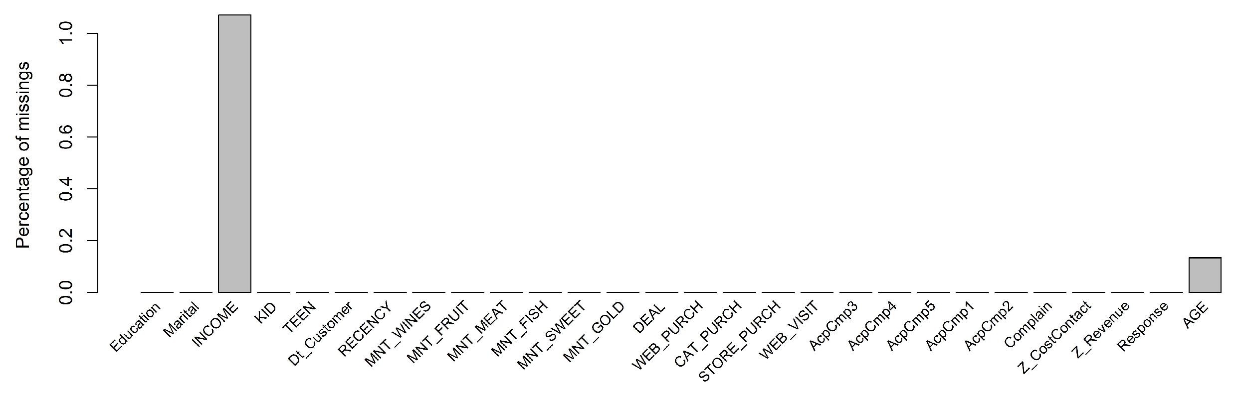
We used several preprocessing procedures to improve data quality and reliability. First, we examined the presence of missing values. Figure 1 presents a bar plot of missing-value percentages across variables. The visualization shows that missing values are mainly concentrated in the INCOME variable (24 observations, 1.07%), while the remaining variables contain no missing observations. In addition, three observations (0.13%) exhibited implausible age values exceeding 100 years. These values were considered data entry errors and were treated as missing prior to imputation.

To formally assess the missingness mechanism, we conducted Little’s MCAR test on key numeric variables (INCOME, AGE, KID, TEEN). The test was not statistically significant (${\chi }_{\left(6\right)}^2=6.17$, $p=0.405$), indicating no evidence against the Missing Completely at Random (MCAR) assumption. Given the very small proportion of missing values (approximately 1%) and the non-significant MCAR test, the missingness mechanism is unlikely to introduce systematic bias, supporting the application of multiple imputation.

Missing data were handled using Multivariate Imputation by Chained Equations (MICE), implemented via the mice package in R, to impute the variables INCOME and AGE. All selected demographic and behavioral variables were included as predictors in the imputation model, with the exception of the customer ID, which was excluded from both prediction and imputation. Given the right-skewed distribution of the INCOME variable, Predictive Mean Matching (PMM) was employed as the imputation method. PMM replaces missing values with observed donor values that have similar predicted means, thereby preserving the empirical distribution and preventing unrealistic extrapolation in the upper tail.

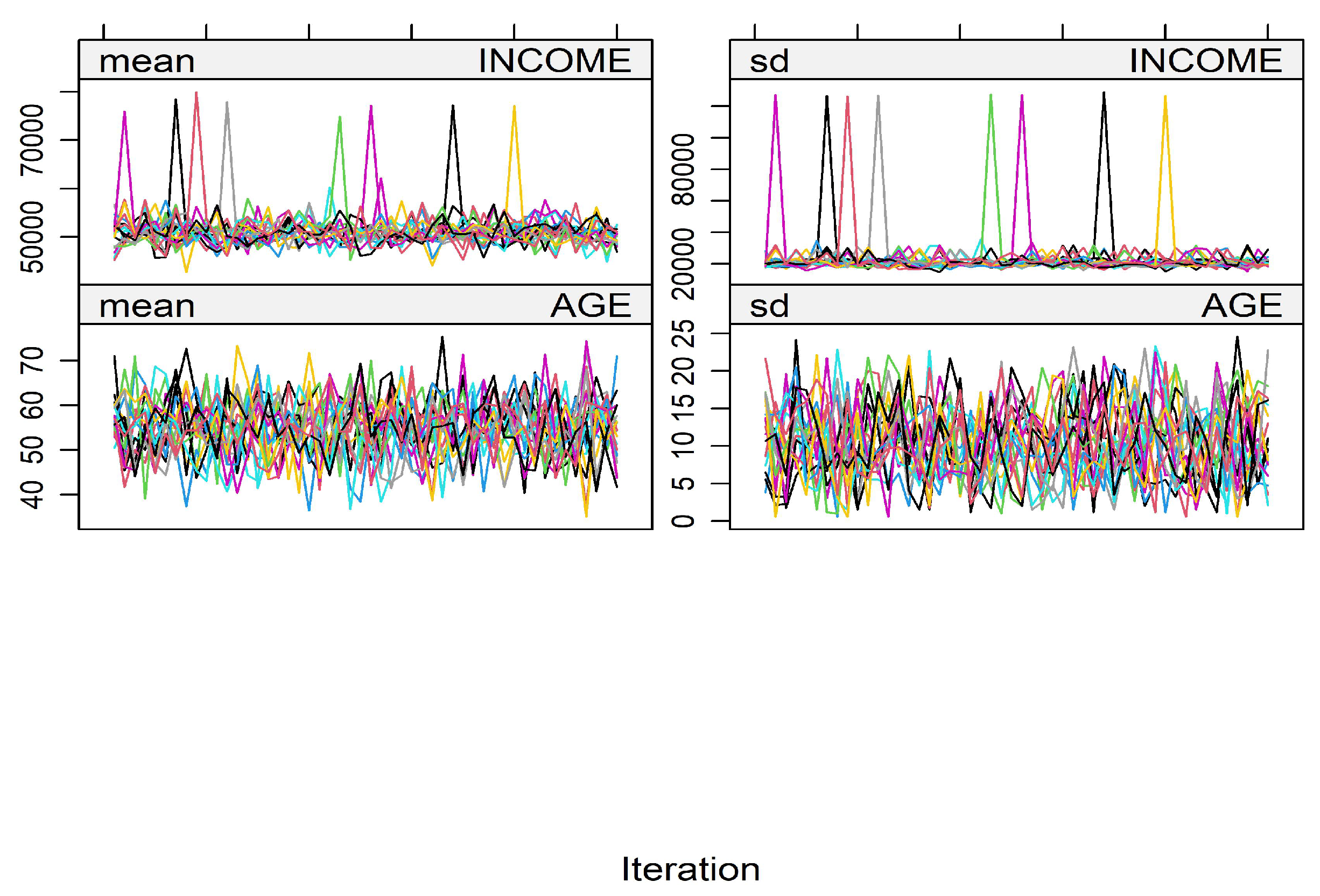
A total of twenty imputed datasets ($m=20$) were generated, with 50 iterations per chain to account for imputation uncertainty. Convergence was assessed using trace plots of summary statistics, namely the mean and standard deviation, across iterations (Figure 2). The resulting trajectories oscillate around stable central values without noticeable upward or downward trends, indicating satisfactory mixing and convergence of the Markov chains.

Throughout the iterations, the mean and standard deviation of both INCOME and AGE remain confined within narrow ranges, with no evidence of persistent drift or divergence between chains. These results suggest that the imputation process attained a stationary distribution and that the chosen number of iterations was sufficient to ensure stable parameter estimates.

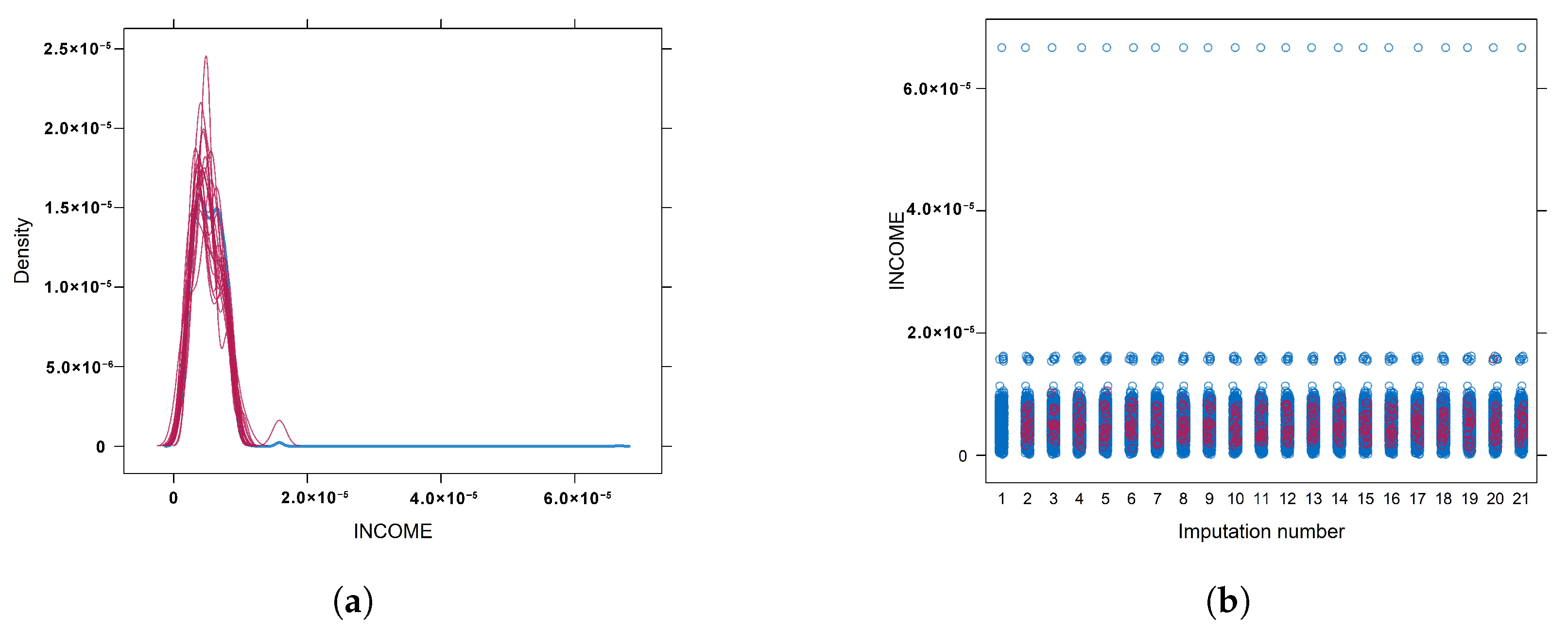
Density overlays comparing observed and imputed values (Figure 3a) show strong overlap between the empirical and imputed distributions. The right-skewed structure of Income is preserved, and no artificial modes or excessive tail inflation are introduced by the imputation procedure. Extreme observed values are retained through PMM, as the method selects donor values from the empirical distribution rather than extrapolating beyond its support.

The strip plot across imputations (Figure 3b) further confirms consistent dispersion patterns among the twenty completed datasets. Imputed values fall within plausible observed ranges, and no systematic shift or concentration is detected in any particular imputation, suggesting stable between-imputation behavior.

To quantify imputation stability, we examined between-imputation variability across the twenty completed datasets.

Table 2. Between-imputation variability of INCOME across $m=20$ completed datasets.

Statistic	Mean Across Imputations	Between-Imputation SD	Range	CV (%)
Mean	52,223.39	16.48	61.12	0.03
Standard Deviation	25,132.02	23.87	105.86	0.09
Median	51,359.50	23.46	113.50	0.05
Q1	35,264.55	68.42	198.00	0.19
Q3	68,513.86	58.86	220.75	0.09

reports the mean of each summary statistic across imputations, the between-imputation standard deviation, the corresponding range, and the coefficient of variation (CV).

The between-imputation variability is negligible relative to the scale of the variable itself. For example, the mean INCOME across imputations is 52,223, with a between-imputation standard deviation of only 16.48 (CV = 0.03%). Similarly, all other statistics exhibit CV values below 0.2%, indicating minimal Monte Carlo variability. These findings indicate that the imputation procedure remains numerically stable and preserves the underlying distributional characteristics of the data.

After imputation, continuous variables were treated for extreme values using Winsorization at the 1st and 99th percentiles via the DescTools package in R. INCOME and AGE exhibited upper-tail dispersion that could inflate pairwise dissimilarities in subsequent analyses. Winsorization replaces extreme values with percentile boundaries while preserving sample size.

To assess the sensitivity of the clustering results to the selected Winsorization thresholds, an additional analysis was performed using alternative trimming levels (2nd–98th percentiles). The resulting clustering structure remained largely consistent with the original solution. The Adjusted Rand Index between the two partitions was 0.783, indicating a high degree of agreement between cluster assignments. Cluster sizes changed only moderately (from 1168–1072 to 1239–1001), suggesting that only a small proportion of boundary observations were reassigned.

Finally, all numeric variables were rescaled to the interval $[0,1]$ interval using Min–Max normalization to ensure comparable contribution in the subsequent Gower distance computation. Continuous variables were normalized after the Winsorization step described above.

3.3. Cluster Analysis

After preprocessing the data, pairwise dissimilarities between observations were computed using the Gower distance. Before constructing the dissimilarity matrix, all numerical variables were scaled to the $[0,1]$ range using Min–Max normalization in order to ensure comparable contributions across variables. This step is consistent with the range-based normalization underlying the Gower formulation and prevents variables with larger scales from dominating the distance computation. Gower distance is well suited for datasets comprising a combination of numerical, categorical, and binary variables. Based on the resulting dissimilarity matrix, agglomerative hierarchical clustering was performed to uncover underlying customer segments. To explore alternative clustering structures, four linkage criteria (Ward.D2, Single, Average, and Complete) were considered. Ward.D2 was applied to the Gower dissimilarity matrix as a variance-minimizing agglomerative criterion. Although Ward.D2 is theoretically derived for squared Euclidean distances, it can also be used with general dissimilarity matrices in hierarchical clustering. In this study, the Gower dissimilarity was used to accommodate the mixed-type structure of the customer dataset. Therefore, Ward.D2 is interpreted here as a practical agglomerative criterion for producing compact and interpretable clusters rather than as a strict variance-minimization procedure in Euclidean space.

The Davies–Bouldin Index (DBI) was employed to evaluate the quality of clustering solutions and guide the selection of the optimal number of clusters. Since the DBI is a centroid-based index defined in Euclidean space, we first applied classical multidimensional scaling (MDS) to the Gower dissimilarity matrix and computed the DBI on the resulting coordinate representation.

The Davies–Bouldin Index offers a global assessment of cluster compactness and separation, while silhouette scores were additionally considered to evaluate the assignment quality at the level of individual observations. The silhouette coefficient was computed directly from the Gower dissimilarity matrix.

The combined use of these metrics enhances the robustness of the clustering results, as DBI captures overall inter-cluster structure, whereas the silhouette measure reflects cohesion and separation for individual data points.

Table 3. Davies-Bouldin Index values computed on a 10-dimensional MDS embedding of the Gower dissimilarity matrix for clustering solutions with $k=2$ to $k=10$. Lower values indicate better cluster compactness and separation.

Linkage	2	3	4	5	6	7	8	9	10
Ward.D2	1.690	2.152	2.304	2.315	2.350	2.480	2.389	2.365	2.256
Single	0.641	0.658	0.656	0.673	0.721	0.873	0.836	0.808	0.821
Average	1.652	1.786	1.579	1.959	1.740	1.791	2.090	2.038	2.041
Complete	1.738	2.094	2.750	2.779	2.742	2.632	2.936	2.843	2.898

reports the Davies–Bouldin index values for clustering solutions with the number of clusters ranging from 2 to 10. For the Ward.D2 linkage, the minimum DBI value (1.690) is observed at $k=2$, indicating that this configuration yields the most suitable clustering solution.

Similarly, both Single and Complete linkage methods achieve their lowest DBI values at $k=2$, whereas the Average linkage attains its minimum at $k=4$. This discrepancy in the selected number of clusters can be attributed to the differing criteria underlying each linkage method. Specifically, Ward.D2 aims to minimize within-cluster variance, while Single linkage is driven by the smallest pairwise distances between observations.

To further examine how strongly the two-cluster solution differs from higher-cluster alternatives, we compared the Ward.D2 results for $k=2$, $k=3$, and $k=4$. As reported in Table 3, the Davies–Bouldin Index increases from 1.690 at $k=2$ to 2.152 and 2.304 for $k=3$ and $k=4$, respectively. In parallel, the mean silhouette coefficient decreases from 0.238 for $k=2$ to 0.182 and 0.183 for $k=3$ and $k=4$. The concurrent degradation of both indices suggests that increasing the number of clusters leads to a decline in overall compactness and separation.

From a practical perspective, higher-cluster solutions mainly subdivide the broader segments identified at $k=2$ rather than revealing clearly distinct customer groups. Although additional clusters could provide finer segmentation granularity, the statistical evidence suggests that these partitions largely reflect boundary splits within existing segments rather than substantively different behavioral profiles. Consequently, the two-cluster solution offers the most balanced combination of statistical quality, structural stability, and managerial interpretability for the present dataset.

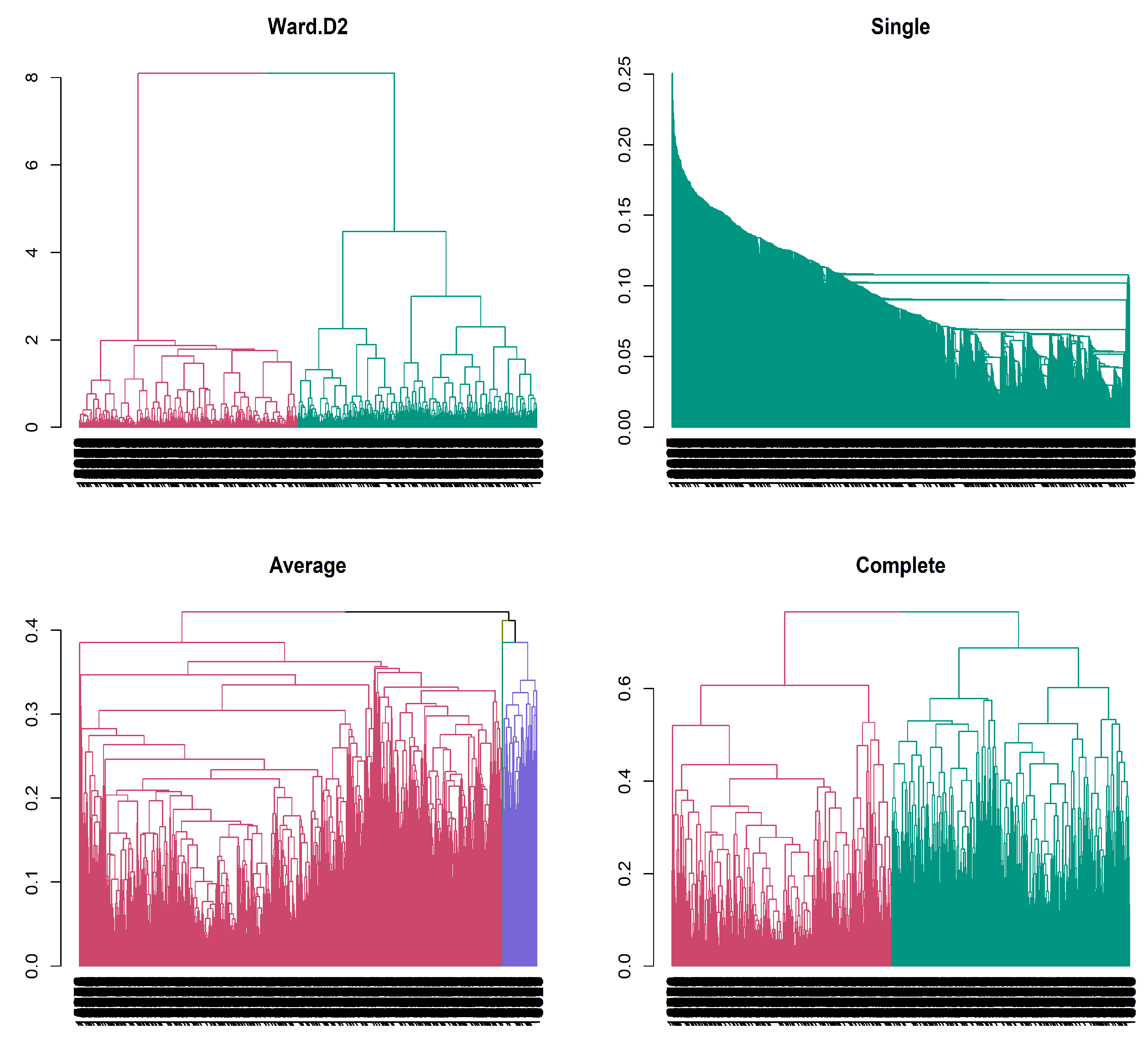
Figure 4 illustrates the outcomes of hierarchical clustering obtained using four different linkage methods. Among these, the Ward.D2 linkage produces clusters that are both compact and well separated. The relatively large linkage heights at which clusters are merged indicate a clear separation between groups.

This behavior can be attributed to the variance-minimizing property of the Ward.D2 method. In contrast, Single linkage relies on minimum pairwise distances, often resulting in chain-like structures, with clusters extending over a wide range of linkage heights. Such patterns reflect weaker separation and reduced clustering quality.

Average linkage, which is based on mean pairwise distances, yields clusters that are moderately compact; however, the resulting structure is less clearly defined compared to Ward.D2. Complete linkage, on the other hand, forms clusters by considering the largest pairwise distances between observations from different clusters. This approach generates compact and well-separated clusters, although it appears less adaptable to the intrinsic structure of the data relative to Ward.D2.

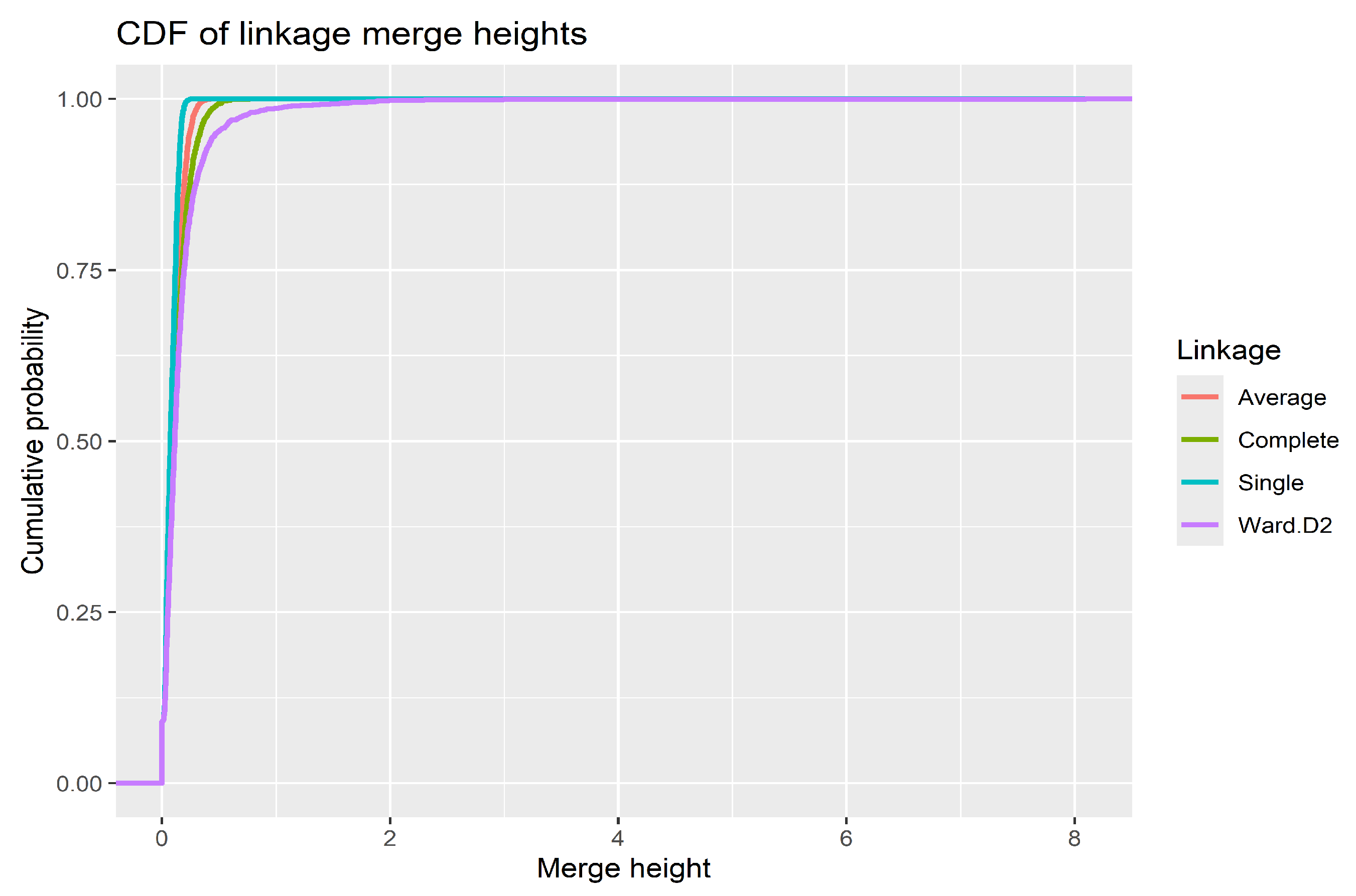
The CDF of merge heights in Figure 5 provides additional insight into the merging behavior of different linkage methods. Ward.D2 consistently generated a more gradual CDF curve compared to the other methods. This pattern indicates that cluster merges occur at higher dissimilarity levels. Single linkage exhibits a rapid increase in linkage height, consistent with its reliance on minimum pairwise distances, which typically leads to chaining effects. By contrast, Ward.D2 displays a more gradual increase, reflecting its variance-minimization criterion that postpones cluster merging until higher dissimilarity levels are reached.

Table 4. Quantitative comparison of hierarchical linkage methods based on the Gower dissimilarity matrix. For each linkage method, the reported partition corresponds to the number of clusters selected by the Davies–Bouldin Index. Mean silhouette values were computed using the Gower dissimilarity matrix.

Linkage Method	Selected k	Mean Silhouette	DBI	Cluster Sizes
Ward.D2	2	0.238	1.690	1168/1072
Single	2	0.300	0.641	2239/1
Average	4	0.235	1.579	2069/167/3/1
Complete	2	0.232	1.738	1164/1076

provides a quantitative comparison of the four hierarchical linkage methods. Although the Single linkage method achieves the highest mean silhouette value and the lowest Davies–Bouldin index, the resulting clustering structure is not meaningful, as it produces one dominant cluster containing almost all observations and a second cluster with only a single observation. A similar issue appears for the Average linkage method, where the optimal solution ($k=4$) leads to several very small clusters. Such highly unbalanced partitions do not represent useful customer segments.

In contrast, both Ward.D2 and Complete linkage produce balanced two-cluster solutions with comparable internal validation values. Among these alternatives, Ward.D2 generates compact clusters with clearer separation and more interpretable group sizes. Therefore, Ward.D2 was selected as the final hierarchical method for the subsequent consensus clustering analysis.

Considering both the Davies–Bouldin Index and the silhouette results, the Ward.D2 method provides an interpretable and structurally meaningful segmentation for the mixed-type customer data. For the selected Ward.D2 solution, the cluster-wise silhouette values were 0.072 for Cluster 1 and 0.420 for Cluster 2, indicating that one cluster forms a cohesive segment while the other represents a broader and more heterogeneous group of customers. Although Cluster 1 has a relatively low silhouette value, additional solutions with $k=3$ and $k=4$ were examined and resulted in worse Davies–Bouldin and silhouette values. This suggests that further splitting mainly subdivides the larger segment without revealing clearly distinct customer groups. Combined with the Davies–Bouldin results and the stability analysis presented in the following subsection, the two-cluster solution provides a parsimonious and practically meaningful segmentation.

Comparison with Alternative Clustering Methods

To examine whether the observed segmentation depends on the clustering algorithm, the hierarchical Ward.D2 solution was compared with two widely used baseline approaches for mixed-type data, Partitioning Around Medoids (PAM) based on the Gower dissimilarity and the K-prototypes algorithm. Prior to the comparison, both baseline methods were explored across different values of k (from $k=2$ to $k=10$). As reported in

Table 5. Exploration of the optimal number of clusters for baseline algorithms.

	PAM		K-Prototypes
$\mathit{k}$	Silhouette	DBI	Silhouette	DBI
2	0.266	1.698	0.287	1.593
3	0.183	2.198	0.221	1.945
4	0.091	2.534	0.212	2.202
5	0.082	2.676	0.196	2.438
6	0.090	2.660	0.130	2.584
7	0.092	2.692	0.121	3.925
8	0.101	2.306	0.110	2.619
9	0.097	2.292	0.110	3.186
10	0.101	2.211	0.090	3.963

, the two-cluster solution consistently yields the highest silhouette values and the lowest Davies–Bouldin indices for both PAM and K-prototypes. This result indicates that the two-cluster structure is not specific to the hierarchical method but is also supported by alternative clustering paradigms. To ensure comparability, all methods were therefore evaluated using the same number of clusters ($k=2$) and identical validation criteria.

Table 6. Comparison of clustering performance between the hierarchical Ward.D2 solution and two baseline algorithms.

Method	Cluster 1 Size	Cluster 2 Size	Mean Silhouette	DBI
Hierarchical (Ward.D2)	1222	1018	0.238	1.690
PAM (Gower)	884	1356	0.266	1.698
K-prototypes	957	1283	0.287	1.593

summarizes the clustering performance of the hierarchical solution and the two baseline algorithms. Among the examined methods, K-prototypes achieves the highest mean silhouette value (0.287) and the lowest Davies–Bouldin index (1.593), indicating slightly stronger internal compactness according to these metrics. PAM also produces a marginally higher mean silhouette value (0.266) compared with the hierarchical solution (0.238), while its Davies–Bouldin index remains similar (1.698).

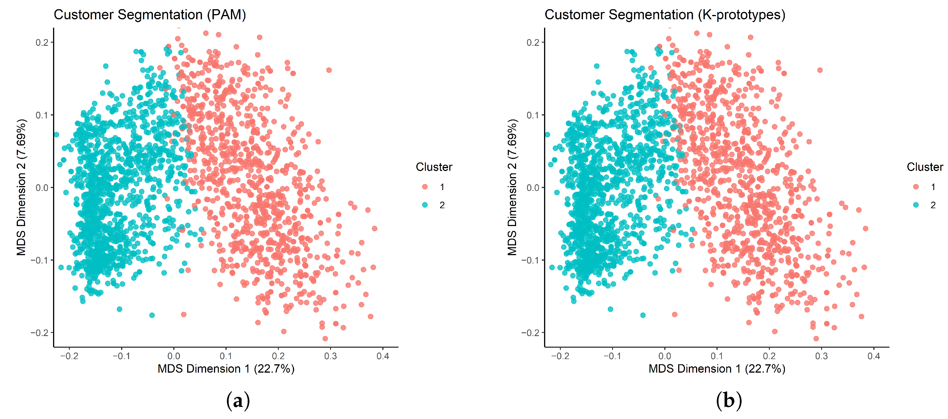
Figure 6 illustrates the clustering structures obtained from the PAM and K-prototypes algorithms in the same two-dimensional MDS embedding of the Gower dissimilarity matrix. In both panels, the separation between the two customer segments occurs primarily along the first MDS dimension, indicating that the dominant partitioning pattern of the dataset is consistently recovered by the two baseline methods. While the K-prototypes solution in Figure 6b exhibits a slightly clearer boundary between the two groups, the PAM solution in Figure 6a shows moderate mixing of observations near the cluster boundary. These differences mainly reflect how the two algorithms assign borderline observations, whereas the overall separation pattern remains largely consistent across the methods.

However, the overall differences between the methods remain relatively small. The mean silhouette values range from 0.238 for the hierarchical solution to 0.287 for K-prototypes, corresponding to a difference of less than 0.05. This suggests that all three algorithms identify a broadly similar segmentation pattern in the data. In other words, the main customer partition appears to be determined primarily by the underlying characteristics of the dataset rather than by the specific clustering algorithm used.

A similar observation emerges from the cluster-wise silhouette values. Across all methods, one cluster consistently forms a compact group with substantially higher silhouette scores, whereas the second cluster exhibits lower cohesion and greater dispersion. The persistence of this asymmetric pattern across multiple algorithms indicates that the customer population contains a relatively homogeneous segment alongside a broader and more heterogeneous group. This structure is typical in behavioral segmentation problems, where a cohesive high-engagement segment coexists with a more diverse general customer population.

Another noticeable difference concerns the distribution of cluster sizes. The hierarchical Ward.D2 solution produces more balanced clusters (1222 and 1018 observations) compared with PAM (884 and 1356) and K-prototypes (957 and 1283). Partition-based algorithms often concentrate observations into a dominant cluster when minimizing within-cluster dispersion, whereas the hierarchical approach preserves a more balanced partition of the data. From a segmentation perspective, such balance facilitates a clearer interpretation of the resulting customer groups.

Overall, although partition-based algorithms achieve slightly stronger internal validation scores, the hierarchical solution produces a highly comparable segmentation structure while preserving the hierarchical relationships among observations. This hierarchical representation becomes particularly useful in the subsequent consensus clustering analysis, where the stability of the segmentation structure is further examined.

3.4. Consensus Trees

Following the initial clustering stage and the evaluation of cluster quality using silhouette scores and the Davies–Bouldin Index (Section 2.3.3), a consensus tree was constructed based on the consensus matrix to enhance the robustness of the identified customer segments.

While DBI and silhouette scores provide insight into cluster compactness and separation, they do not explicitly capture clustering stability. To address this limitation, a subsampling-based consensus clustering framework was implemented, employing hierarchical clustering with Ward.D2 linkage over $B=500$ resampling iterations.

According to the DBI and silhouette results, $k=2$ was initially selected as the optimal number of clusters. The subsequent consensus analysis reinforced this choice, indicating that the two-cluster configuration yields the most stable and parsimonious segmentation. Such stability is essential for reliable customer profiling.

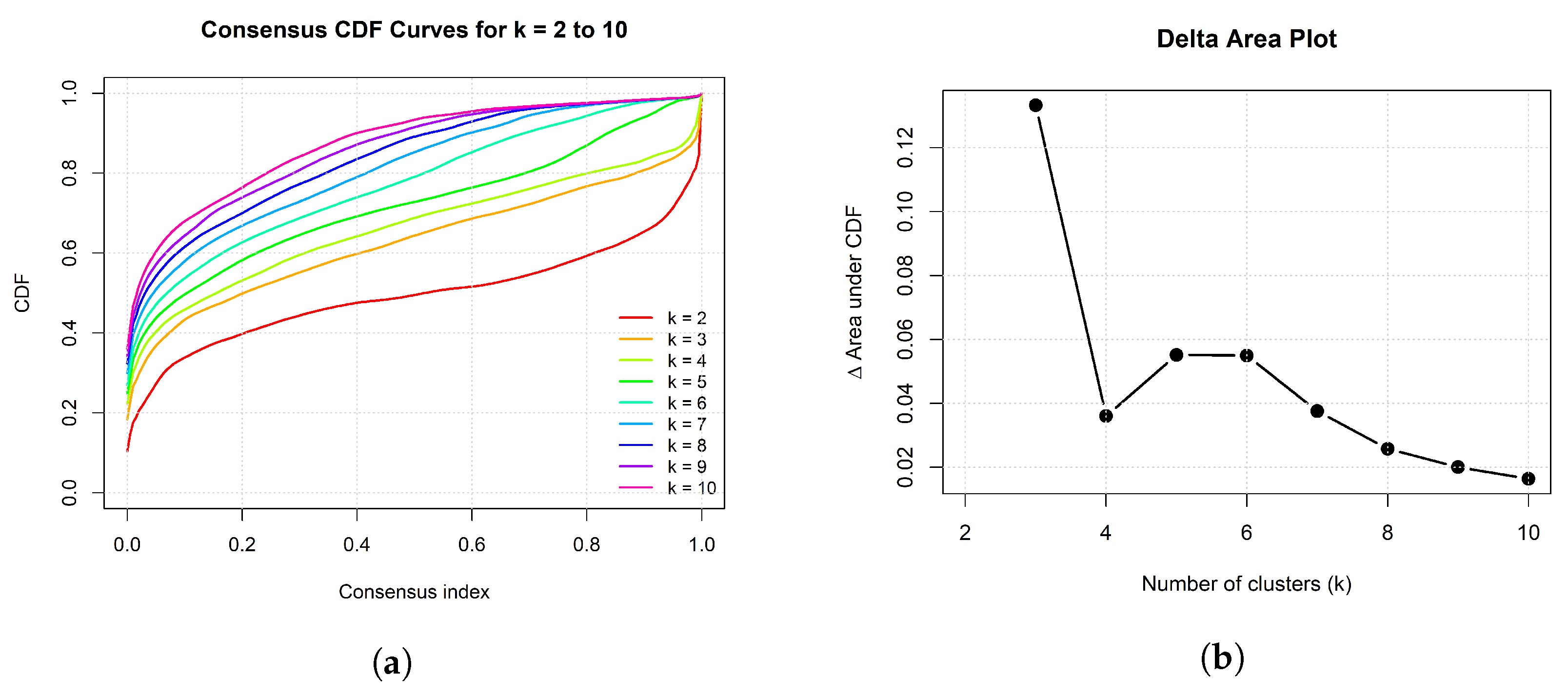
Figure 7 displays the consensus cumulative distribution function (CDF) curves for $k=2$ to $k=10$ (Figure 7a), along with the corresponding Delta Area plot (Figure 7b), which captures the variation in the area under the CDF curve across successive values of k.

The most pronounced increase in the area occurs at $k=3$ (i.e., from $k=2$ to $k=3$, $\mathrm{\Delta }A=0.134$). Beyond this point, the curve stabilizes, with only marginal improvements observed (e.g., $\mathrm{\Delta }A=0.034$ at $k=4$ and values below $0.056$ thereafter). Considering both the Delta Area and the CDF behavior, $k=2$ emerges as the most stable and parsimonious clustering solution.

In addition to the CDF and Delta area plots, we computed the Proportion of Ambiguous Clustering (PAC) to further evaluate clustering stability. PAC quantifies the proportion of consensus values lying in an intermediate interval (0.1–0.9), with lower values indicating greater clustering stability. As reported in

Table 7. Proportion of Ambiguous Clustering (PAC) values for consensus clustering with $k=2$ to $k=10$. Lower values indicate higher clustering stability.

Number of Clusters (k)	PAC Value
2	0.302
3	0.374
4	0.366
5	0.440
6	0.439
7	0.401
8	0.372
9	0.338
10	0.303

, the lowest PAC value is observed for $k=2$ (PAC = 0.3023), although the value for $k=10$ (PAC = 0.3029) is numerically very close.

Across the examined values of k, the PAC values do not follow a strictly monotonic decreasing pattern and exhibit moderate fluctuations. In particular, higher PAC values are observed around $k=5$ and $k=6$, indicating a larger proportion of ambiguous pairwise assignments and suggesting that these partitions may contain less stable cluster boundaries.

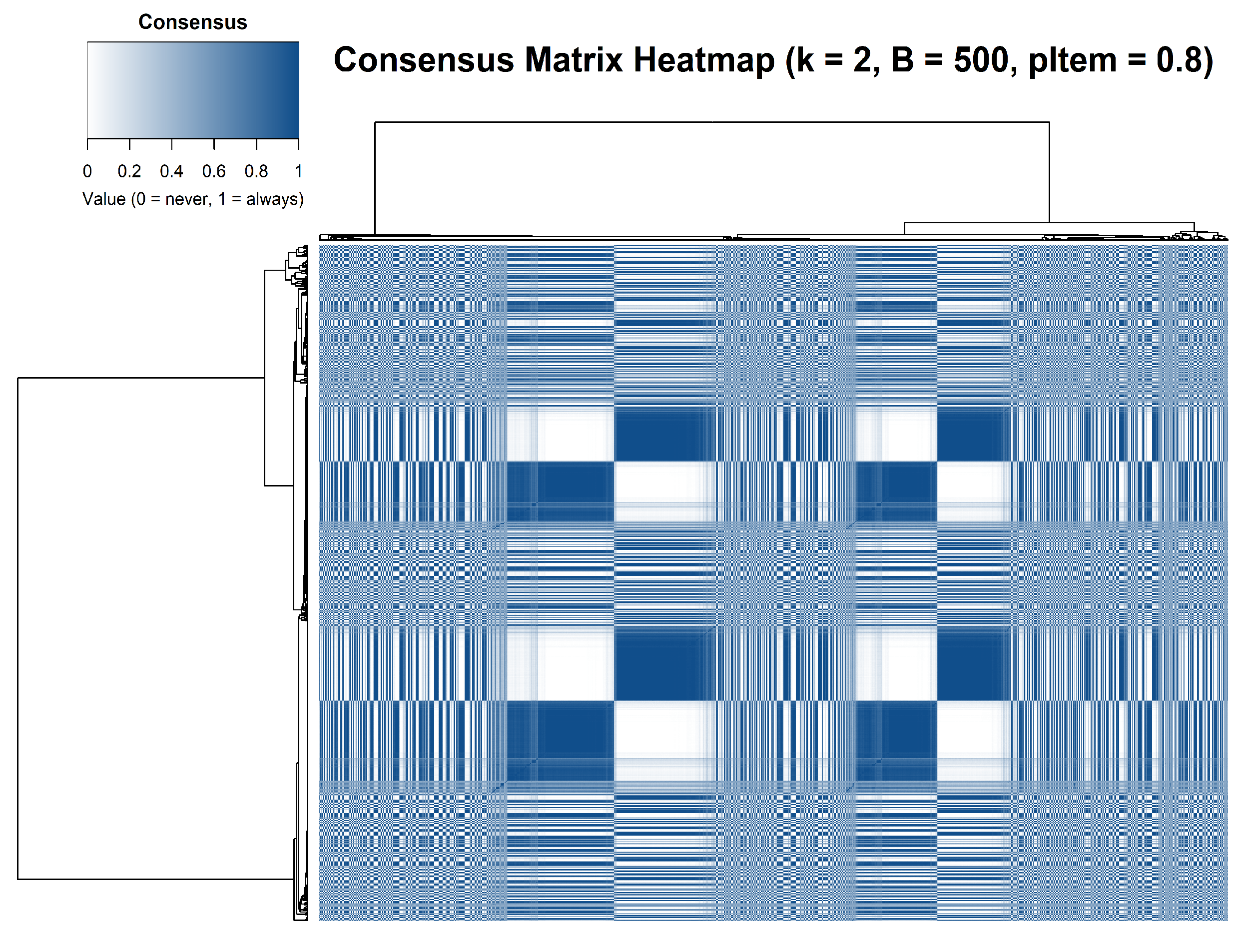
Although the PAC value for $k=2$ is around 0.30, this level of ambiguity is expected in behavioral segmentation settings where boundary observations naturally occur between customer groups. The consensus heatmap in Figure 8 still exhibits a clear block structure, indicating that most pairwise assignments remain stable across subsampling iterations.

However, the final choice of the number of clusters was not based solely on PAC values. The Davies–Bouldin Index (Table 3) and silhouette analysis both indicate that $k=2$ provides the most compact and well-separated structure for the Ward.D2 solution. In addition, the Delta area plot shows that the most substantial increase in the area under the CDF curve occurs when moving from $k=2$ to $k=3$, after which the gains become marginal. Considering these complementary criteria together with the principle of parsimony and interpretability of the resulting segments, the two-cluster solution was selected as the most appropriate partition.

To quantify the variability of the stability diagnostics across subsampling iterations, we examined the empirical distributions of PAC and Delta area obtained during the consensus procedure. Because consensus clustering itself relies on repeated subsampling, the variability of these indices can be directly estimated from the resampling trajectories. As summarized in

Table 8. Empirical variability of consensus stability diagnostics across subsampling iterations.

Statistic	Mean	SD	2.5%	97.5%
PAC ($k=2$)	0.316	0.0029	0.310	0.320
PAC ($k=10$)	0.304	0.0010	0.302	0.305
$\mathrm{\Delta }$Area ($k=3$)	0.136	0.0004	0.135	0.137
$\mathrm{\Delta }$Area ($k=4$)	0.035	0.0004	0.034	0.035

, for the selected two-cluster solution the PAC value has an empirical mean of 0.316 with a 95% interval of [0.310, 0.320]. Similarly, the largest increase in the area under the CDF occurs at $k=3$, with a mean Delta area of 0.136 and a 95% interval of [0.135, 0.137]. These narrow intervals indicate that the stability diagnostics remain highly consistent across subsampled datasets and therefore support the robustness of the identified clustering structure.

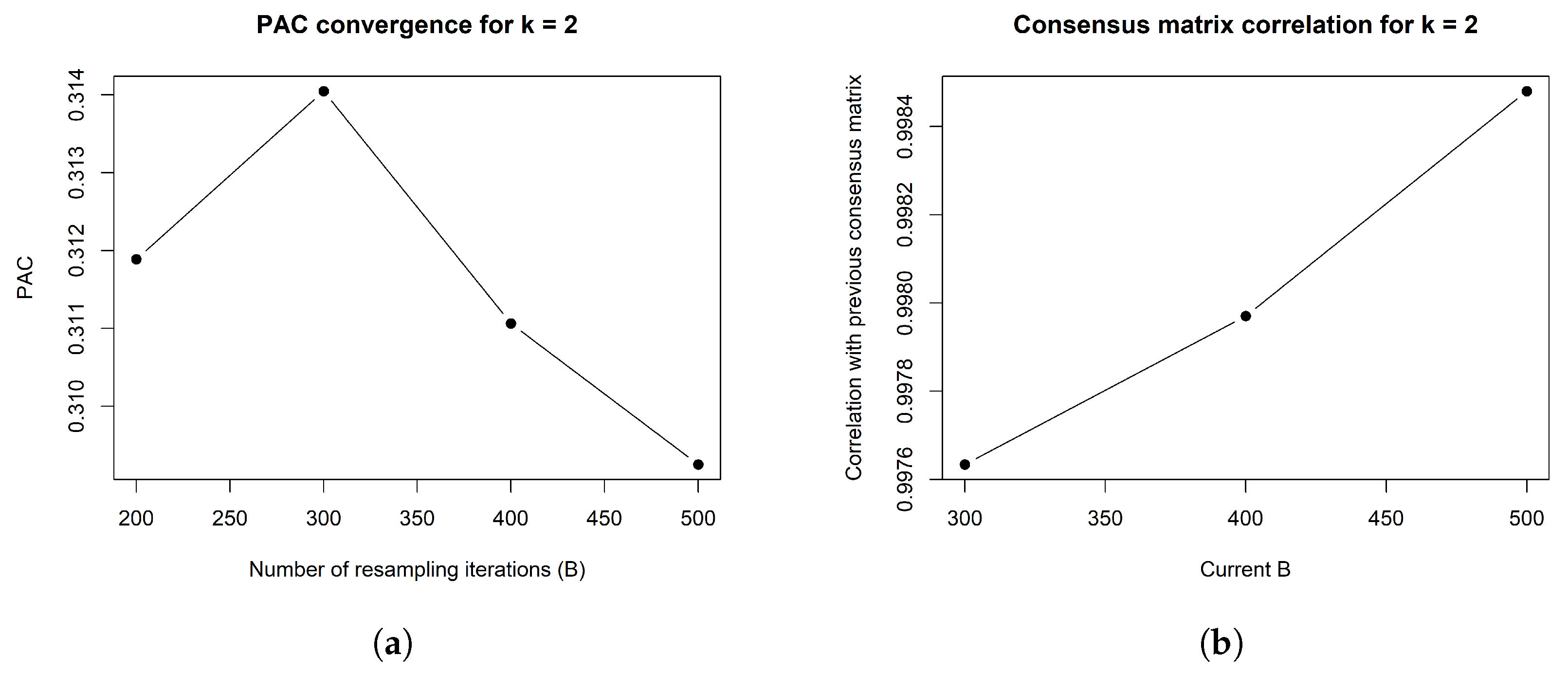
To further examine the convergence of the consensus procedure, we evaluated the stability of the consensus matrix across increasing numbers of resampling iterations. Specifically, the consensus matrix for the selected solution ($k=2$) was recomputed using $B=200,300,400,$ and 500 resampling iterations. The convergence diagnostics include the Proportion of Ambiguous Clustering (PAC), the correlation between successive consensus matrices, and the relative Frobenius change between consecutive matrices.

As shown in

Table 9. Convergence diagnostics of the consensus clustering procedure for $k=2$.

B	PAC	Correlation with Previous	Relative Frobenius Change
200	0.3119	–	–
300	0.3140	0.9976	0.0442
400	0.3111	0.9980	0.0409
500	0.3093	0.9985	0.0355

and Figure 9a, PAC values remain highly stable across the examined iteration levels. In addition, Figure 9b shows that the correlation between successive consensus matrices remains above 0.997 and slightly increases as B grows, while the relative Frobenius change gradually decreases. These diagnostics suggest that the consensus matrix becomes increasingly stable as the number of resampling iterations grows, supporting the use of $B=500$ in the final analysis.

Once the optimal number of clusters is determined, the consensus matrix is derived from the proportion of resampling iterations in which each pair of individuals $(i,j)$ is grouped within the same cluster. The corresponding hierarchical structure is then obtained from the pairwise dissimilarity matrix defined as $(1-C)$.

Figure 8 presents the heatmap of the consensus matrix for $k=2$, where each entry reflects how frequently two observations are assigned to the same cluster across $B=500$ resampling iterations. The resulting heatmap reveals two well-defined blocks along the diagonal, indicating strong within-cluster agreement among customers across repeated subsampling runs.

The block pattern observed in the consensus matrix indicates stable within-cluster assignments and reinforces the reliability of the two-cluster solution. The relatively clear separation between the two main blocks indicates that the clustering structure is reasonably stable, although some intermediate consensus values suggest the presence of boundary observations.

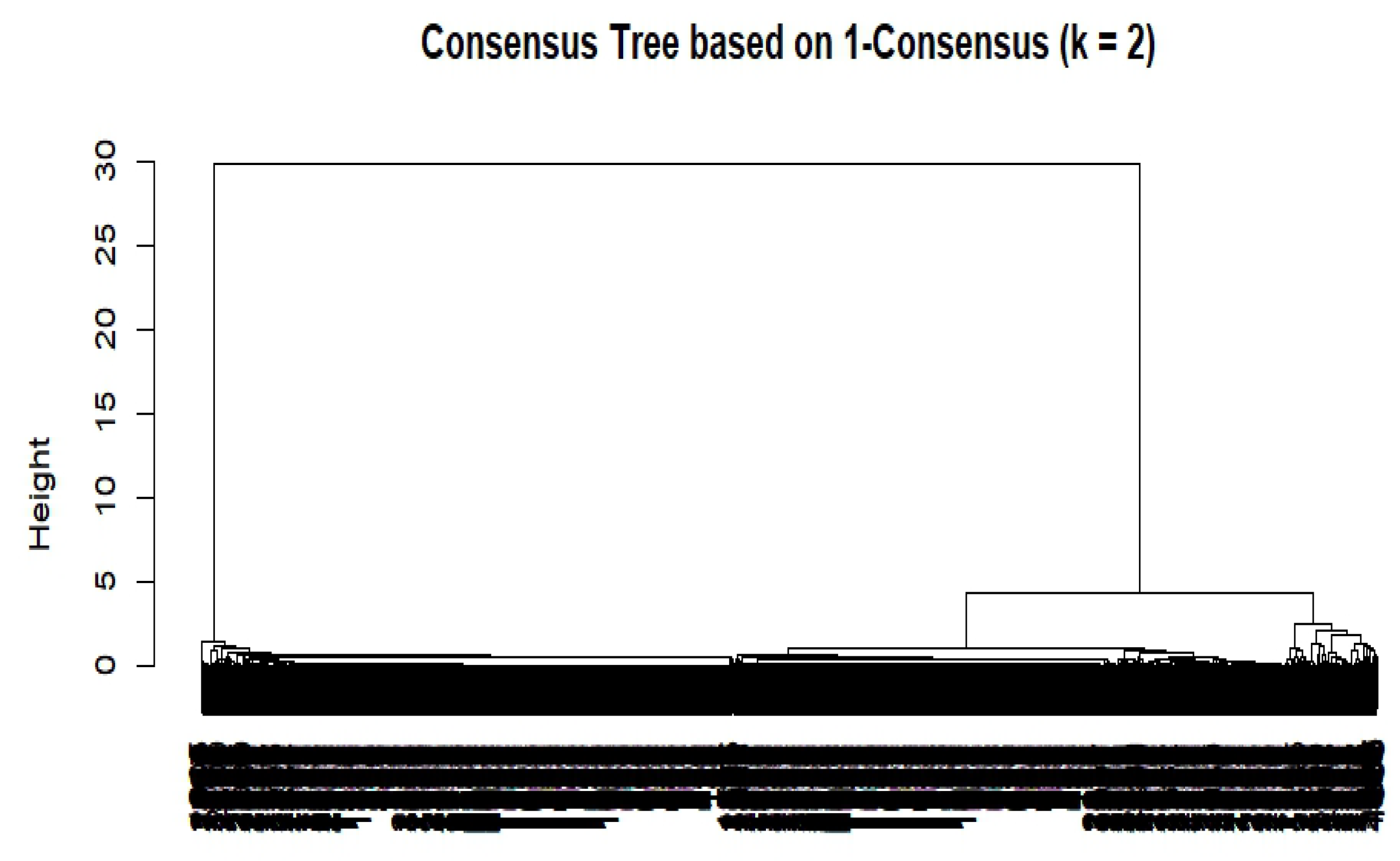
To further investigate the hierarchical organization of the identified customer segments, a consensus tree was constructed from the dissimilarity matrix $(1-C)$, as shown in Figure 10. The resulting dendrogram exhibits a clear bipartite structure, with two primary branches corresponding to the extracted clusters.

The height at which these main branches merge represents the degree of dissimilarity between the clusters. The branch that separates at the highest level in the dendrogram corresponds to a group of customers that is more distinct in terms of behavioral characteristics compared to the other segment. Such differences may be associated with variations in purchasing intensity, demographic profiles, or engagement patterns.

Branches that merge at lower heights correspond to finer within-cluster variations, suggesting that while the overall two-cluster structure is stable, there remains heterogeneity within each segment.

3.5. Customer Segment Analysis

Behavioral profiling was conducted for the two-cluster solution obtained from the consensus clustering procedure.

Table 10. Summary of customer behavioral and demographic profiles across consensus clusters ($k=2$), based on mean normalized values (scaled to $[0,1]$) for spending behavior, household structure, and channel activity.

Variables	Cluster 1 (n = 1222)	Cluster 2 (n = 1018)
Avg_INCOME	0.673	0.309
Avg_MNT_WINES	0.405	0.031
Avg_MNT_GOLD	0.294	0.072
Avg_MNT_FISH	0.277	0.031
Avg_MNT_MEAT	0.304	0.028
Avg_MNT_FRUITS	0.256	0.028
Avg_MNT_SWEET	0.254	0.029
Avg_KID	0.082	0.390
Avg_TEEN	0.280	0.221
Avg_DEAL	0.253	0.202
Avg_CAT_PURCH	0.410	0.054
Avg_STORE_PURCH	0.545	0.107
Avg_WEB_PURCH	0.515	0.194
Avg_WEB_VISIT	0.219	0.322
Avg_RECENCY	0.493	0.500
Avg_AGE	0.538	0.436

summarizes the mean normalized values of the main profiling variables for each segment.

The results indicate a clear behavioral separation between the two clusters. Cluster 1 ($n=1222$) represents a higher-value customer segment characterized by substantially higher purchasing intensity and spending levels across all product categories. For instance, normalized INCOME is markedly higher in Cluster 1 (0.673) compared with Cluster 2 (0.309). A similar pattern is observed for product expenditures. Wine spending in Cluster 1 (0.405) is more than ten times greater than in Cluster 2 (0.031), while meat expenditure (0.304 vs. 0.028), fish (0.277 vs. 0.031), fruits (0.256 vs. 0.028), sweets (0.254 vs. 0.029), and gold products (0.294 vs. 0.072) all show substantial differences between the two groups. These results indicate that customers in Cluster 1 consistently exhibit stronger consumption patterns across all product categories.

Purchasing channel activity follows a similar pattern. Customers in Cluster 1 demonstrate considerably higher engagement in both physical and digital purchasing channels. Store purchases are substantially higher in Cluster 1 (0.545) than in Cluster 2 (0.107), while catalog purchases (0.410 vs. 0.054) and web purchases (0.515 vs. 0.194) also show clear differences. In contrast, web visits are more frequent in Cluster 2 (0.322 vs. 0.219), suggesting that customers in this segment interact with the online platform more often but convert these visits into purchases less frequently.

Demographic characteristics also show differences between the two segments. Customers in Cluster 2 have a noticeably higher presence of children in the household (KID = 0.390) compared with Cluster 1 (0.082). This household structure may partially explain the lower discretionary spending observed in this segment. Age differences are more moderate, with Cluster 1 showing a slightly higher normalized mean age (0.538) than Cluster 2 (0.436).

To statistically assess these differences between the two segments, Wilcoxon rank-sum tests were conducted for each profiling variable comparing the two clusters. The resulting p-values were adjusted using the Benjamini–Hochberg procedure, and rank-biserial correlations were computed as effect size measures. The results

Table 11. Statistical comparison of selected profiling variables between the two consensus clusters using Wilcoxon rank–sum tests. Adjusted p-values were computed using the Benjamini–Hochberg procedure, and effect sizes are reported as rank-biserial correlations.

Variable	Cluster 1	Cluster 2	p-Value	Adj. p	Effect Size
INCOME	0.673	0.309	<0.001	<0.001	0.777
MNT_WINES	0.405	0.031	<0.001	<0.001	0.836
MNT_MEAT	0.304	0.028	<0.001	<0.001	0.796
STORE_PURCH	0.545	0.107	<0.001	<0.001	0.811
WEB_PURCH	0.515	0.194	<0.001	<0.001	0.721
WEB_VISIT	0.219	0.322	<0.001	<0.001	0.423
KID	0.082	0.390	<0.001	<0.001	0.585
RECENCY	0.493	0.500	0.581	0.581	0.012

confirm that most spending and purchasing variables differ significantly between the two clusters with large effect sizes, particularly for income (effect size = 0.777), wine expenditure (0.836), store purchases (0.811), and web purchases (0.721). These large effect magnitudes indicate that the separation between the clusters reflects substantial behavioral differences rather than minor statistical variations.

In contrast, the RECENCY variable shows very similar values across the two segments (0.493 vs. 0.500) and does not exhibit a statistically significant difference. This suggests that the segmentation structure is primarily driven by differences in purchasing intensity and overall spending behavior rather than by the timing of the most recent purchase.

Overall, the analysis reveals two clearly differentiated customer segments: a higher-value group characterized by stronger purchasing engagement and higher expenditure levels, and a lower-spending segment with weaker purchasing activity and greater browsing behavior. This structure provides a parsimonious and interpretable customer segmentation that can support targeted marketing strategies.

3.6. Assigning New Customers to the Identified Clusters

From an operational perspective, new customers can be assigned to the identified segments using a nearest-medoid rule based on the Gower dissimilarity. For each cluster, the corresponding medoid was identified from the training data, and each new observation was assigned to the cluster whose medoid yielded the smallest Gower distance.

To evaluate the performance of this assignment procedure, we conducted a hold-out validation using an 80% training and 20% test split. The resulting confusion matrix (

Table 12. Classification performance of the nearest-medoid rule for assigning new customers to clusters.

	Actual Cluster 1	Actual Cluster 2
Predicted Cluster 1	223	8
Predicted Cluster 2	22	196
Accuracy	0.933
Precision (Cluster 1)	0.965
Recall (Cluster 1)	0.910
Precision (Cluster 2)	0.899
Recall (Cluster 2)	0.961

) indicates that 223 observations from Cluster 1 and 196 observations from Cluster 2 were correctly classified, whereas 22 and 8 observations were misclassified, respectively. The overall classification accuracy reached 0.933. Precision and recall were also high for both clusters (Cluster 1: precision = 0.965, recall = 0.910; Cluster 2: precision = 0.899, recall = 0.961), indicating that the proposed rule provides a reliable operational mechanism for assigning new customers to the identified segments.

4. Discussion

In this study, we proposed a hierarchical clustering approach for mixed-type customer data based on the combination of Gower dissimilarity, Ward.D2 linkage and subsampling-based consensus validation. This approach allows heterogeneous variable types to be handled simultaneously, accounts for scale differences, and enables the evaluation of clustering stability.

The DBI, computed on the MDS embedding of the Gower dissimilarity matrix and complemented by silhouette analysis, initially indicated that a two-cluster structure provides the most compact and well-separated solution. The subsequent consensus-based stability analysis reinforced the selection of $k=2$ as the simplest and most robust partition based on CDF, Delta area and the minimum PAC among candidate solutions. In addition, the comparison with alternative clustering algorithms (PAM based on Gower dissimilarity and the K-prototypes method) revealed a highly similar two-segment structure, indicating that the identified partition is not specific to the hierarchical algorithm but rather reflects an intrinsic structure of the dataset.

The resulting segmentation reveals two structurally distinct customer groups characterized by clear differences in normalized income, purchasing intensity, and channel engagement. These differences were further supported by non-parametric statistical tests, which confirmed that the majority of behavioral variables differ significantly between the two clusters with substantial effect sizes. One segment exhibits consistently higher expenditure across product categories and stronger transactional behavior, whereas the second segment is characterized by lower spending levels and higher browsing activity relative to actual purchases. The cluster-wise silhouette analysis also indicated that one segment forms a more cohesive group, while the second segment represents a broader and more heterogeneous population of customers.

From a methodological viewpoint, the incorporation of hierarchical clustering with consensus-based validation improves the reliability of unsupervised segmentation results in mixed-type datasets. The resulting structure is stable and interpretable, thus well-suited for high-dimensional consumer analytics and related applications.

Future research may extend this framework by incorporating neutrosophic logic into the consensus clustering approach. The current method measures stability, but it does not explicitly model uncertainty or account for conflicting patterns that may appear across different resampling runs. In the present framework, several sources of uncertainty may arise during the analysis. First, the multiple imputation procedure generates several plausible versions of the dataset, reflecting uncertainty associated with missing values [52]. Second, the subsampling-based consensus clustering approach may produce slightly different cluster assignments across resampling iterations, as clustering structures can vary depending on the sampled observations [1]. Finally, observations located near cluster boundaries may exhibit ambiguous membership, which is often reflected by lower silhouette values and weaker separation between clusters [49].

While the current framework evaluates clustering stability through consensus analysis, it does not explicitly represent such indeterminacy. In this context, a neutrosophic extension could provide a way to explicitly represent these sources of uncertainty by introducing a triplet structure that captures cluster stability, indeterminacy in boundary assignments, and conflicting patterns observed across resampling runs.

Indeed, a neutrosophic consensus structure could assign to each candidate partition a triplet $(T,I,F)$ representing stability, uncertainty, and falsity. These measures could then guide hierarchical aggregation, pruning decisions, and adaptive threshold, thereby leading to more flexible and uncertainty-aware segmentation models.

References

1. Monti, S.; Tamayo, P.; Mesirov, J.; Golub, T. Consensus Clustering: A Resampling-Based Method for Class Discovery and Clustering Validation. Mach. Learn. 2003, 52, 91–118. [Google Scholar] [CrossRef]
2. Lancichinetti, A.; Fortunato, S. Consensus Clustering in Complex Networks. Sci. Rep. 2012, 2, 336. [Google Scholar] [CrossRef]
3. Ben-Hur, A.; Elisseeff, A.; Guyon, I. A Stability Based Method for Discovering Structure in Clustered Data. Biocomputing 2002, 7, 6–17. [Google Scholar] [CrossRef]
4. Hennig, C. Cluster-Wise Assessment of Cluster Stability. Comput. Stat. Data Anal. 2007, 52, 258–271. [Google Scholar] [CrossRef]
5. Hennig, C.; Meila, M.; Murtagh, F.; Rocci, R. Handbook of Cluster Analysis; CRC Press: Boca Raton, FL, USA, 2015. [Google Scholar] [CrossRef]
6. Gower, J.C. A General Coefficient of Similarity and Some of Its Properties. Biometrics 1971, 27, 857–871. [Google Scholar] [CrossRef]
7. Wedel, M.; Kamakura, W.A. Market Segmentation: Conceptual and Methodological Foundations; Springer: Berlin/Heidelberg, Germany, 2000. [Google Scholar] [CrossRef]
8. Lock, E.F.; Dunson, D.B. Bayesian Consensus Clustering. Bioinformatics 2013, 29, 2610–2616. [Google Scholar] [CrossRef]
9. Coleman, S.; Kirk, P.D.W.; Wallace, C. Consensus Clustering for Bayesian Mixture Models. BMC Bioinform. 2022, 23, 483. [Google Scholar] [CrossRef] [PubMed]
10. Margush, T.; McMorris, F.R. Consensusn-Trees. Bull. Math. Biol. 1981, 43, 239–244. [Google Scholar] [CrossRef]
11. Bombelli, I.; Ferraro, M.B.; Vichi, M. Consensus and Fuzzy Partition of Dendrograms from a Three-Way Dissimilarity Array. Inf. Sci. 2023, 637, 118948. [Google Scholar] [CrossRef]
12. Hu, T.; Sung, S.Y. Consensus Clustering. Intell. Data Anal. 2005, 9, 551–565. [Google Scholar] [CrossRef]
13. Ward, J.H. Hierarchical Grouping to Optimize an Objective Function. J. Am. Stat. Assoc. 1963, 58, 236–244. [Google Scholar] [CrossRef]
14. Gao, L.L.; Bien, J.; Witten, D. Selective Inference for Hierarchical Clustering. J. Am. Stat. Assoc. 2024, 119, 332–342. [Google Scholar] [CrossRef] [PubMed]
15. Oggier, F.; Datta, A. Renyi Entropy Driven Hierarchical Graph Clustering. PeerJ Comput. Sci. 2021, 7, e366. [Google Scholar] [CrossRef]
16. Grégoire, G. Elements of Statistics. EAS Publ. Ser. 2016, 77, 13–37. [Google Scholar] [CrossRef]
17. Adugna, T.D.; Ramu, A.; Haldorai, A. A Review of Pattern Recognition and Machine Learning. J. Mach. Comput. 2024, 4, 210–220. [Google Scholar] [CrossRef]
18. Lloyd, S.P. Least Squares Quantization in PCM. IEEE Trans. Inf. Theory 1982, 28, 129–137. [Google Scholar] [CrossRef]
19. Zubair, M.; Iqbal, M.A.; Shil, A.; Chowdhury, M.J.M.; Moni, M.A.; Sarker, I.H. An Improved k-Means Clustering Algorithm Towards an Efficient Data-Driven Modeling. Ann. Data Sci. 2022, 11, 1525–1544. [Google Scholar] [CrossRef]
20. Kanungo, T.; Mount, D.M.; Netanyahu, N.S.; Piatko, C.D.; Silverman, R.; Wu, A.Y. An Efficient k-Means Clustering Algorithm: Analysis and Implementation. IEEE Trans. Pattern Anal. Mach. Intell. 2002, 24, 881–892. [Google Scholar] [CrossRef]
21. Haldane, J.B.S. Note on the Median of a Multivariate Distribution. Biometrika 1948, 35, 414–415. [Google Scholar] [CrossRef]
22. Godichon-Baggioni, A.; Surendran, S. A Penalized Criterion for Selecting the Number of Clusters for K-Medians. J. Comput. Graph. Stat. 2024, 33, 1298–1309. [Google Scholar] [CrossRef]
23. Huang, Z. Extensions to the k-Means Algorithm for Clustering Large Data Sets with Categorical Values. Data Min. Knowl. Discov. 1998, 2, 283–304. [Google Scholar] [CrossRef]
24. Gavva, S.T.; Karthik, C.S.; Punna, S. Clustering Categorical Data: Soft Rounding k-Modes. Inf. Comput. 2024, 296, 105115. [Google Scholar] [CrossRef]
25. Kaufman, L.; Rousseeuw, P.J. Finding Groups in Data: An Introduction to Cluster Analysis; John Wiley & Sons: New York, NY, USA, 1991. [Google Scholar] [CrossRef]
26. Yue, H.; Ali, M.M.; Lin, Y.; Liu, H. Ultra-Short-Term Forecasting of Large Distributed Solar PV Fleets Using Sparse Smart Inverter Data. IEEE Trans. Sustain. Energy 2024, 15, 1968–1980. [Google Scholar] [CrossRef]
27. Huang, Z. Clustering Large Data Sets with Mixed Numeric and Categorical Values. In Proceedings of the First Pacific-Asia Conference on Knowledge Discovery and Data Mining (PAKDD); World Scientific: Singapore, 1997; pp. 21–34. [Google Scholar]
28. Campello, R.J.G.B.; Kröger, P.; Sander, J.; Zimek, A. Density-Based Clustering. Wiley Interdiscip. Rev. Data Min. Knowl. Discov. 2020, 10, e1343. [Google Scholar] [CrossRef]
29. Ester, M.; Kriegel, H.P.; Sander, J.; Xu, X. A Density-Based Algorithm for Discovering Clusters in Large Spatial Databases with Noise. In Proceedings of the Second International Conference on Knowledge Discovery and Data Mining (KDD-96); AAAI Press: Washington, DC, USA, 1996; pp. 226–231. [Google Scholar]
30. Kanagala, H.K.; Krishnaiah, V.V.J.R. A Comparative Study of k-Means, DBSCAN and OPTICS. In Proceedings of the International Conference on Computing, Communication and Informatics (ICCCI 2016); IEEE: New York, NY, USA, 2016; pp. 1–6. [Google Scholar] [CrossRef]
31. Bouveyron, C.; Celeux, G.; Murphy, T.B.; Raftery, A.E. Model-Based Clustering and Classification for Data Science: With Applications in R; Cambridge University Press: Cambridge, UK, 2019. [Google Scholar] [CrossRef]
32. Fraley, C.; Raftery, A.E. Model-Based Clustering, Discriminant Analysis, and Density Estimation. J. Am. Stat. Assoc. 2002, 97, 611–631. [Google Scholar] [CrossRef]
33. Gormley, I.C.; Murphy, T.B.; Raftery, A.E. Model-Based Clustering. Annu. Rev. Stat. Its Appl. 2023, 10, 573–595. [Google Scholar] [CrossRef]
34. Smarandache, F. Neutrosophic Set: A Generalization of the Intuitionistic Fuzzy Set. Int. J. Pure Appl. Math. 2005, 24, 287–297. [Google Scholar]
35. Rashno, E.; Minaei-Bidgoli, B.; Guo, Y. An Effective Clustering Method Based on Data Indeterminacy in Neutrosophic Set Domain. Eng. Appl. Artif. Intell. 2020, 89, 103411. [Google Scholar] [CrossRef]
36. Guo, Y.; Sengur, A. A novel image segmentation algorithm based on neutrosophic c-means clustering. Expert Syst. Appl. 2014, 41, 594–602. [Google Scholar] [CrossRef]
37. Koundal, D. Texture-Based Image Segmentation Using Neutrosophic Clustering. IET Image Process. 2017, 11, 640–645. [Google Scholar] [CrossRef]
38. Ashika, T.; Grace, H.; Martin, N.; Smarandache, F. Enhanced Neutrosophic Set and Machine Learning Approach for Breast Cancer Prediction. Neutrosophic Sets Syst. 2024, 73. [Google Scholar] [CrossRef]
39. Wani, A.A. Comprehensive Analysis of Clustering Algorithms: Exploring Limitations and Innovative Solutions. PeerJ Comput. Sci. 2024, 10, e2286. [Google Scholar] [CrossRef] [PubMed]
40. Larose, D.T.; Larose, C.D. Discovering Knowledge in Data; Wiley: Hoboken, NJ, USA, 2014. [Google Scholar] [CrossRef]
41. Mathew, T.; Rencher, A.C. Methods of Multivariate Analysis; Wiley: New York, NY, USA, 1996. [Google Scholar]
42. Carta, S.; Consoli, S.; Piras, L.; Podda, A.S.; Recupero, D.R. Event Detection in Finance Using Hierarchical Clustering Algorithms on News and Tweets. PeerJ Comput. Sci. 2021, 7, 1–39. [Google Scholar] [CrossRef]
43. Day, W.; McMorris, F. A Formalization of Consensus Index Methods. Bull. Math. Biol. 1985, 47, 215–229. [Google Scholar] [CrossRef]
44. Bryant, D. A Classification of Consensus Methods for Phylogenetics. In Bioconsensus; Janowitz, M., Lapointe, F.J., McMorris, F., Mirkin, B., Roberts, F., Eds.; American Mathematical Society: Providence, RI, USA, 2003; pp. 163–184. [Google Scholar] [CrossRef]
45. Steel, M. Phylogeny: Discrete and Random Processes in Evolution; SIAM: Bangkok, Thailand, 2016. [Google Scholar] [CrossRef]
46. Fred, A.L.N.; Jain, A.K. Combining Multiple Clusterings Using Evidence Accumulation. IEEE Trans. Pattern Anal. Mach. Intell. 2005, 27, 835–850. [Google Scholar] [CrossRef] [PubMed]
47. Strehl, A.; Ghosh, J. Cluster Ensembles: A Knowledge Reuse Framework for Combining Multiple Partitions. J. Mach. Learn. Res. 2002, 3, 583–617. [Google Scholar]
48. Davies, D.L.; Bouldin, D.W. A Cluster Separation Measure. IEEE Trans. Pattern Anal. Mach. Intell. 1979, 1, 224–227. [Google Scholar] [CrossRef]
49. Rousseeuw, P.J. Silhouettes: A Graphical Aid to the Interpretation and Validation of Cluster Analysis. J. Comput. Appl. Math. 1987, 20, 53–65. [Google Scholar] [CrossRef]
50. Şenbabaoğlu, Y.; Michailidis, G.; Li, J.Z. Critical Limitations of Consensus Clustering in Class Discovery. Sci. Rep. 2014, 4, 6207. [Google Scholar] [CrossRef]
51. Wilkerson, M.D.; Hayes, D.N. ConsensusClusterPlus: A Class Discovery Tool with Confidence Assessments and Item Tracking. Bioinformatics 2010, 26, 1572–1573. [Google Scholar] [CrossRef]
52. Rubin, D.B. Multiple Imputation for Nonresponse in Surveys; Wiley: Hoboken, NJ, USA, 1987. [Google Scholar] [CrossRef]
Figure 1. Percentage of missing values across variables. Missingness is mainly concentrated in the INCOME variable, with a small percentage also observed in AGE due to implausible values treated as missing.
Mathematics 14 01294 g001
Figure 2. Trace plots of mean and standard deviation for Income and Age across MICE iterations. Different colors represent independent chains; their substantial overlap indicates good mixing and convergence and does not affect readability.
Mathematics 14 01294 g002
Figure 3. Diagnostic plots evaluating the stability and distributional consistency of the multiple imputation procedure for Income. (a) Density comparison between observed and imputed values, where different colors represent imputations and their overlap indicates close agreement with the empirical distribution while preserving the right-skewed structure. (b) Strip plot across the m = 20 completed datasets, illustrating the dispersion of imputed values and the absence of systematic shifts between imputations. Scientific notation is used for axis labels.
Mathematics 14 01294 g003
Figure 4. Dendrograms obtained using four linkage methods (Ward.D2, Single, Average, and Complete). Branch colors indicate cluster membership after cutting the dendrogram at the selected number of clusters for each linkage method.
Mathematics 14 01294 g004
Figure 5. Cumulative distribution functions (CDFs) of dissimilarities obtained from different linkage methods (Average, Complete, Single, and Ward.D2).
Mathematics 14 01294 g005
Figure 6. Clustering structures obtained from the two baseline algorithms. Both methods identify a similar separation pattern between the two customer segments when projected onto the same MDS representation of the Gower dissimilarity matrix. (a) PAM clustering visualized in the two-dimensional MDS embedding of the Gower dissimilarity matrix; (b) K-prototypes clustering visualized in the same MDS embedding.
Mathematics 14 01294 g006
Figure 7. Consensus clustering diagnostics. (a) Cumulative Density Function (CDF) for k = 2 , , 10 ; (b) Delta area plot showing the relative increase in area under the CDF curve.
Mathematics 14 01294 g007
Figure 8. Consensus matrix heatmap for k = 2 clusters over B = 500 resampling iterations.
Mathematics 14 01294 g008
Figure 9. Convergence diagnostics of the consensus clustering procedure for k = 2 . (a) PAC values across increasing resampling iterations; (b) Correlation between successive consensus matrices.
Mathematics 14 01294 g009
Figure 10. Consensus Tree constructed from the dissimilarity matrix ( 1 C ) for k = 2 , where height indicates the level of between-cluster dissimilarity.
Mathematics 14 01294 g010