A Lightweight Improved RT-DETR for Stereo-Vision-Based Excavator Posture Recognition

Abstract

In intelligent excavator applications, traditional excavator posture recognition methods face two major challenges: limited recognition accuracy and insufficient computing resources on edge devices. To address these issues, this study proposes an excavator posture recognition method based on an improved Real-Time Detection Transformer (RT-DETR). First, a new backbone network is designed based on the Reparameterized Vision Transformer to improve feature utilization efficiency while reducing computational demands. Next, the overall architecture is optimized by introducing lightweight Dynamic Upsamplers, which reduce information loss during upsampling and enhance multi-scale feature fusion. In addition, a Cross-Attention Fusion Module is adopted to strengthen local feature extraction while retaining the global modeling capability of the Transformer, thereby improving the discrimination between foreground and background. Finally, a Multi-Scale Fusion Network is introduced to further enhance the multi-scale feature representation ability of RT-DETR. Experimental results show that the proposed method achieves a mean average precision (mAP) of 94.29% for small object detection, which is 7.96% higher than that of the baseline RT-DETR, while reducing the number of model parameters by 34.95%. Compared with YOLO-series models, the proposed method improves mAP by 8.62% to 12.75%. These results indicate that the proposed method outperforms existing methods in both detection accuracy and computational efficiency and provides an efficient and feasible solution for real-time excavator posture recognition.

1. Introduction

Hydraulic excavators are widely used in mining, forestry, construction, and many other fields because of their high efficiency, versatility, and robust performance. In addition to excavating soil to form trenches or holes, hydraulic excavators can also be used for grading, heavy lifting, and transportation tasks. However, construction sites are often characterized by harsh and hazardous working conditions, and accidents may result in severe injuries to workers and substantial property losses. Therefore, over the past two decades, researchers have shown increasing interest in intelligent excavators. The use of intelligent excavators in such hazardous environments can not only improve productivity but also significantly enhance operational safety [1].

To realize the intelligence of hydraulic excavators, high-precision pose perception is a key enabling technology. At present, pose measurement systems mainly follow two technical routes: contact-based and non-contact-based methods. Contact-based measurement relies on embedded sensor networks. For example, dynamic inclinometers are used to collect the boom pitch angle in real time, while magnetostrictive displacement sensors integrated into hydraulic cylinders are employed to obtain the motion parameters of the stick [2,3,4]. Through subsequent data calculation and processing, the pose data of the excavator can then be obtained [5,6]. Although this physically contact-based measurement approach has the theoretical advantage of direct measurement, it exhibits significant technical limitations in practical engineering applications. Specifically, the sensors are susceptible to high-frequency vibrations caused by nonlinear hydraulic shocks and compound motions of the excavator, which introduce time-varying noise into the signal acquisition system. In addition, the inherent limitations of the mechanical structure lead to the accumulation of measurement errors, thereby severely affecting system stability.

Although traditional contact-based sensor methods can alleviate the effects of vibration and impact in specific scenarios through passive vibration-reduction structures, it remains difficult to avoid measurement degradation and the risk of equipment damage in complex construction environments. In contrast, non-contact measurement methods based on computer vision demonstrate stronger robustness and adaptability. These methods can achieve high-precision pose estimation without physical contact, effectively avoiding the influence of vibration and environmental interference. Moreover, they do not require complicated sensor deployment and maintenance, thereby reducing the overall hardware cost and system failure rate. Machine vision systems can also provide long-term continuous monitoring, making them particularly suitable for construction tasks in high-risk and harsh environments and offering a more forward-looking solution for intelligent control systems [5].

Jiayue Zhao et al. [7] performed excavator posture estimation based on the YOLOv5 model and achieved automatic recognition of excavator posture. However, due to the limited local receptive field of convolutional neural networks, the model accuracy was still insufficient. In addition, because the model relies on non-maximum suppression (NMS) for post-processing, its computational complexity is relatively high, which makes deployment on edge devices difficult. Yapeng Guo et al. [8], by contrast, adopted a lightweight fully convolutional network (FCN) for excavator posture recognition. Although this approach effectively reduced the demand for computational resources, the problem of insufficient accuracy still remained.

To effectively address the large posture recognition errors and high computational requirements of existing methods and to further improve the intelligence and safety performance of excavators, this paper introduces the RT-DETR object detection algorithm and combines it with stereo vision for hydraulic excavator posture recognition. Furthermore, the RT-DETR algorithm is structurally optimized and improved in this study to achieve better performance in small-object detection while reducing the computational burden on devices, thus providing a more efficient and feasible solution for engineering applications.

The main contributions are summarized as follows:

1.

A posture angle recognition method for excavator working devices is proposed, and an integrated technical pipeline is established, consisting of coded marker detection, binocular vision-based 3D coordinate recovery, world coordinate transformation, and geometric solving of posture angles. By combining the layout of coded markers, the 3D point cloud information from the ZED stereo camera, and the D–H kinematic model, the proposed method enables the calculation of the posture angles of the boom, stick, and bucket.

2.

To address the large number of parameters and high computational cost of RT-DETR in edge-device deployment, RepViT is introduced as a lightweight backbone network. This reduces model complexity and inference burden while improving the feature extraction capability for small targets.

3.

To overcome the limitation of traditional bilinear interpolation in preserving sufficient detail during upsampling, the DySample dynamic upsampling operator is introduced, allowing the sampling positions to be learned adaptively. This enhances multi-scale feature fusion and improves small-target detection performance.

4.

A convolution-and-attention fusion module (CAFM) is designed to combine the local detail modeling capability of convolution with the global context modeling capability of the attention mechanism, thereby improving the discriminability between target markers and background under complex backgrounds.

5.

A multi-scale feed-forward network (MSFN) is designed to enhance multi-scale feature representation through dilated convolution, depthwise separable convolution, and a gated fusion mechanism, further improving the model’s detection accuracy and robustness for small targets in complex scenes.

2. Related Work

2.1. Object Detectors

YOLOv1 [9] was the first single-stage object detector based on a convolutional neural network (CNN), achieving truly real-time object detection. After years of continuous development, the YOLO family has surpassed other single-stage object detectors [10,11] and has become almost synonymous with real-time object detection. YOLO detectors can generally be divided into two categories: anchor-based methods [11,12,13,14] and anchor-free methods [15,16,17,18]. These methods achieve a reasonable balance between speed and accuracy and have been widely applied in various practical scenarios. However, these advanced real-time detectors usually generate a large number of overlapping bounding boxes and require non-maximum suppression (NMS) as a post-processing step, which in turn reduces their inference speed.

End-to-end object detectors, by contrast, are well known for their simplified detection pipeline. Carion et al. [19] first proposed the Transformer-based end-to-end detector, Detection Transformer (DETR), which attracted widespread attention because of its unique design. In particular, DETR discards manually designed anchor boxes and the NMS component and instead adopts bipartite matching to directly predict a one-to-one set of objects. Nevertheless, DETR still suffers from several issues, such as slow training convergence and difficulty in query optimization. To address these problems, many DETR variants have been proposed. Deformable DETR [20] accelerates training convergence by improving the efficiency of the attention mechanism and exploiting multi-scale features. DAB-DETR [21] and DN-DETR [22] further improve performance by introducing iterative box refinement and denoising training, respectively. Group-DETR [23] introduces a group-based many-to-one assignment strategy. Among these variants, RT-DETR [24] exhibits the most competitive overall performance. Therefore, RT-DETR is selected as the baseline model in this study.

2.2. Excavator Marker Design

To achieve accurate measurement of the posture of the excavator working mechanism, this system adopts a three-dimensional visual posture measurement scheme specifically designed to measure the angular positions of the boom, stick, and bucket. Accordingly, feature markers that can be easily recognized by a stereo camera system are mounted on each key component to reflect its posture angle information [25,26]. Each marker adopts a binary-coded structure composed of a square and a circle. The centerline of the circle is parallel to the measured component and is used to assist in posture direction recognition, whereas the square is responsible for the encoding function. To ensure unique encoding, each side of the square is divided into three equal parts, and different binary sequences are formed through the presence or absence of line segments. Specifically, a missing line segment represents “0”, whereas a present line segment represents “1”, thereby forming a recognizable edge pattern.

Contour distortion may occur in stereo camera views because of imaging angles. However, the overall deformation of these feature markers in images is relatively small, which facilitates reliable recognition and detection (see Figure 1). In particular, in the posture measurement of the boom and stick, the inclination angle of the extracted saddle-point line in the marker can accurately reflect the posture angle of the corresponding working component, thereby enabling high-precision measurement and dynamic tracking.

3. Excavator Posture Recognition Method

3.1. Improved Real-Time Detection Transformer

Real-Time Detection Transformer Base Model

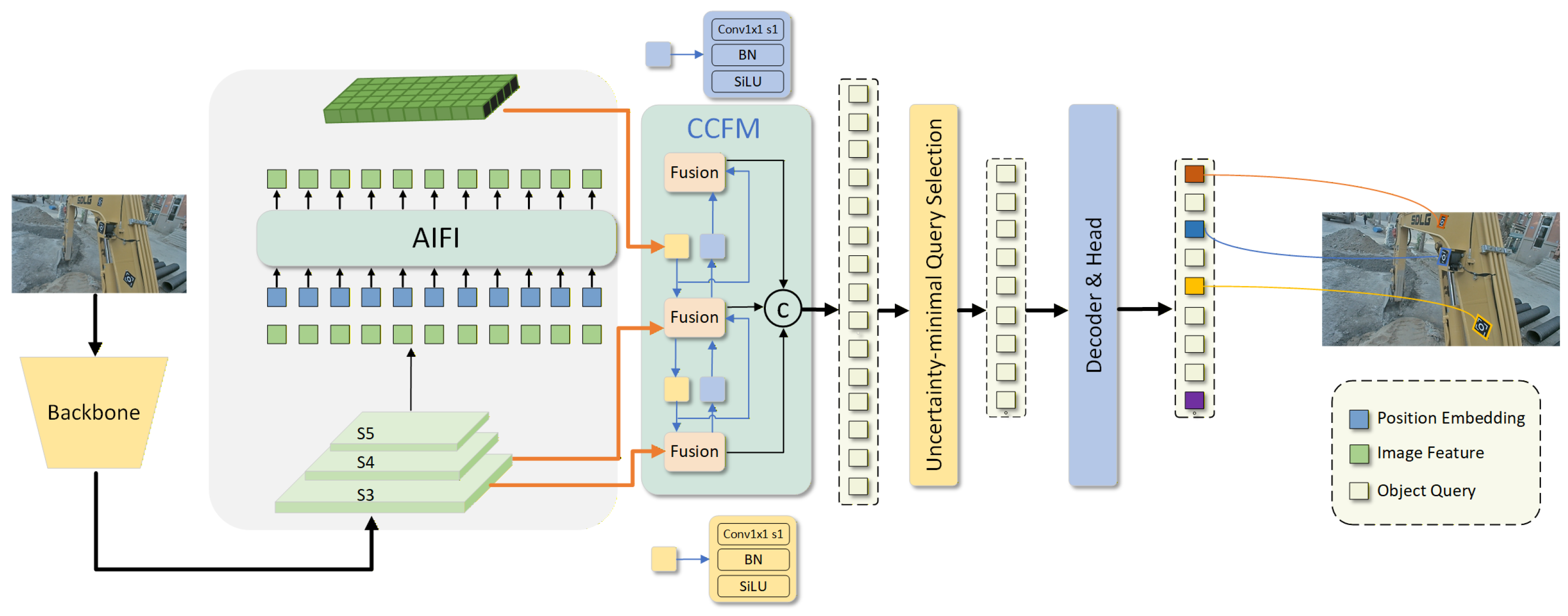
Real-Time Detection Transformer (RT-DETR) is an end-to-end detector specifically designed for real-time object detection. This method significantly improves detection accuracy and speed by employing an efficient hybrid encoder to process multi-scale features and incorporating a query selection mechanism based on uncertainty minimization. Through the self-attention mechanism, RT-DETR can capture long-range dependencies and effectively distinguish small objects in complex backgrounds. In contrast, traditional methods such as YOLOv5 and SSD are limited by the local receptive field of CNNs, and the insufficient resolution of deep features often leads to the loss of small-object information. Meanwhile, RT-DETR eliminates the anchor-box mechanism and NMS post-processing and instead adopts a dynamic detection head to directly predict object locations, thereby avoiding the problems of redundant anchor matching and erroneous suppression by NMS in dense scenes. By comparison, two-stage models such as Faster R-CNN rely on region proposals and RoI pooling, resulting in high computational cost and insufficient sensitivity to small-object feature extraction. Therefore, RT-DETR is selected for object detection in this study. The main focus of this paper is to optimize the performance of RT-DETR for small-object detection and to further improve its lightweight design so as to reduce the computational burden. By optimizing the network architecture, the proposed method aims to achieve accurate small-object detection while reducing model complexity and enabling lightweight processing.

First, the features from the last three stages of the backbone are taken as inputs and fed into the efficient hybrid encoder. Through the AIFI-based cross-scale feature interaction and the cross-scale feature fusion module (CCFM), the multi-scale features are transformed into a series of image features. Then, a fixed number of image features are selected as the initial object queries for the decoder by using the IoU-aware query selection method. Finally, the decoder equipped with auxiliary prediction heads iteratively refines the object queries to generate bounding boxes and confidence scores. The network architecture is shown in Figure 2.

3.2. Improvements to Real-Time Detection Transformer

In the practical process of recognizing visual markers on the excavator working device, such as the bucket, boom, and stick, the target markers often undergo deformation, blur, or partial occlusion because the working device is in frequent motion, which increases the difficulty of detection. At the same time, RT-DETR still has relatively high parameter complexity and computational cost, which limits its deployment and real-time application on resource-constrained embedded platforms.

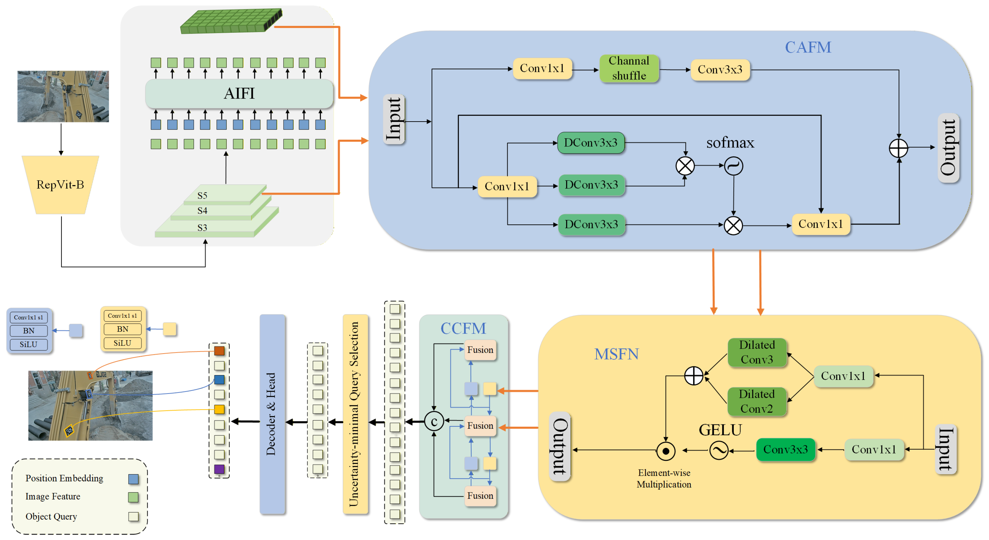
To address the above issues, this study systematically optimizes the RT-DETR model with the aim of improving its small-object detection accuracy in complex scenarios while reducing its computational cost to meet real-time requirements. First, a lightweight backbone network is designed based on the Reparameterized Vision Transformer (RepViT) to reduce computation and inference latency, making the model more suitable for resource-constrained environments while enhancing its feature extraction capability. Second, the original bilinear interpolation in the model is optimized using DySample, so that multi-scale information can be captured more effectively without introducing excessive additional parameters. Then, a Convolution and Attention Fusion Module (CAFM) is introduced to fuse local and global features. Finally, a Multiscale Feed-Forward Network (MSFN) is added to aggregate multi-scale features and improve the model’s accuracy and robustness in complex backgrounds. The overall architecture of the improved model is shown in Figure 3.

Lightweight Backbone Based on RepViT

At present, as the complexity of detection algorithms continues to increase, the number of parameters and the computational cost also grow accordingly, which poses a considerable challenge for embedded devices with limited computing resources. In practical application scenarios, embedded devices are often deployed under resource-constrained and harsh environmental conditions. Therefore, how to reduce the inference burden of the algorithm while maintaining detection performance has become an urgent issue to be addressed.

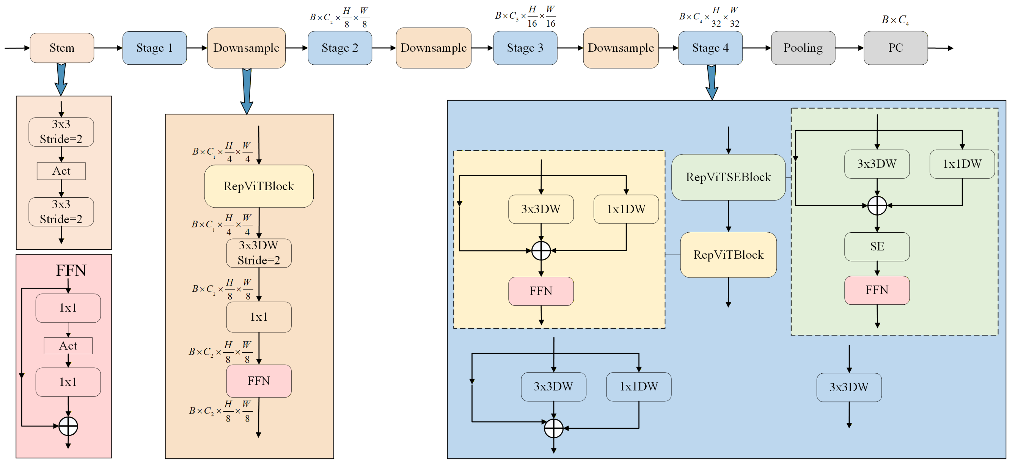
For RT-DETR, although the Detection Transformer has been optimized for real-time performance, the convolutional neural network backbone it employs (e.g., ResNet) still contains a relatively large number of parameters for embedded devices. Therefore, Reparameterized Vision Transformer (RepViT) is introduced as the backbone of RT-DETR to further improve inference speed while minimizing the loss of detection accuracy. Its structure is shown in Figure 4.

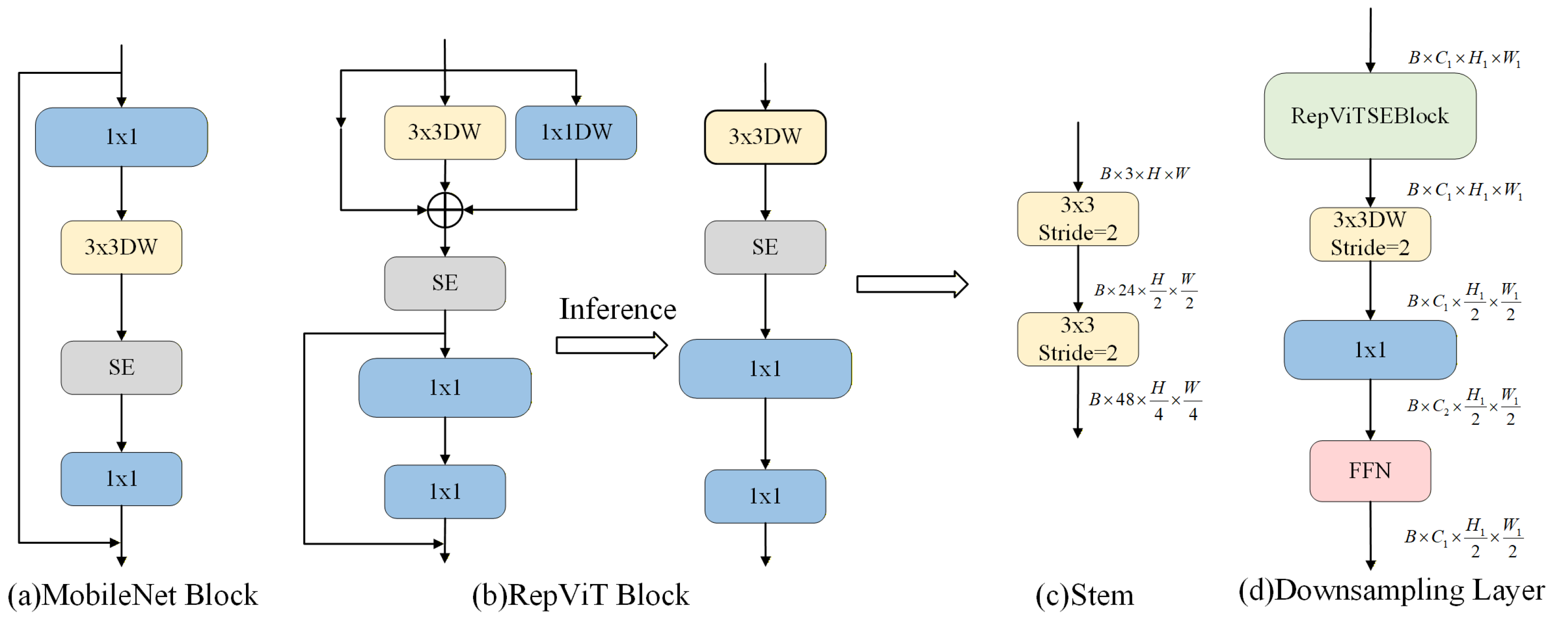
In the stem stage, RepViT adopts two $3\times 3$ convolutions with a stride of 2 for downsampling (as shown in Figure 5c). In each stage, the input features are extracted through two RepViT blocks. The RepViT block is optimized based on the MobileNetV3 module by decoupling the token mixer and the channel mixer. Specifically, the depthwise convolution (DW) layer is moved forward, while the squeeze-and-excitation (SE) layer is placed after the DW layer, as illustrated in the improved structure shown in Figure 5b. In addition, during feature map downsampling, RepViT adopts an independent downsampling module (as shown in Figure 5d), in which a RepViT module is first applied, followed by a $3\times 3$ depthwise convolution and a $1\times 1$ convolution in sequence. Finally, a feed-forward network (FFN) module is connected.

In the stem stage, this method captures more fine-grained details by using convolutions, thereby reducing resolution loss and preserving detailed information. Two successive $3\times 3$ convolutions with a stride of 2 are equivalent to extracting features layer by layer with overlapping windows. Since each step downsamples the feature map by only a factor of 2, more spatial resolution of small objects is preserved before the features enter deeper layers of the network, which is beneficial for detecting small-sized targets. Moreover, the $3\times 3$ convolution naturally provides local translation invariance and smooth transition capability, enabling continuous modeling of relationships among neighboring pixels. By decoupling the token mixer and the channel mixer, the RepViT block allows the token mixer to focus on local spatial information aggregation, with computational complexity growing linearly with spatial resolution, while the channel mixer focuses on channel-wise interaction, with computation depending only on the number of channels. This design not only improves the efficiency of feature extraction but also effectively reduces computational complexity. Meanwhile, the independent downsampling layer preserves rich contextual information during resolution reduction, thereby enhancing feature representation capability at low resolutions.

3.3. DySample

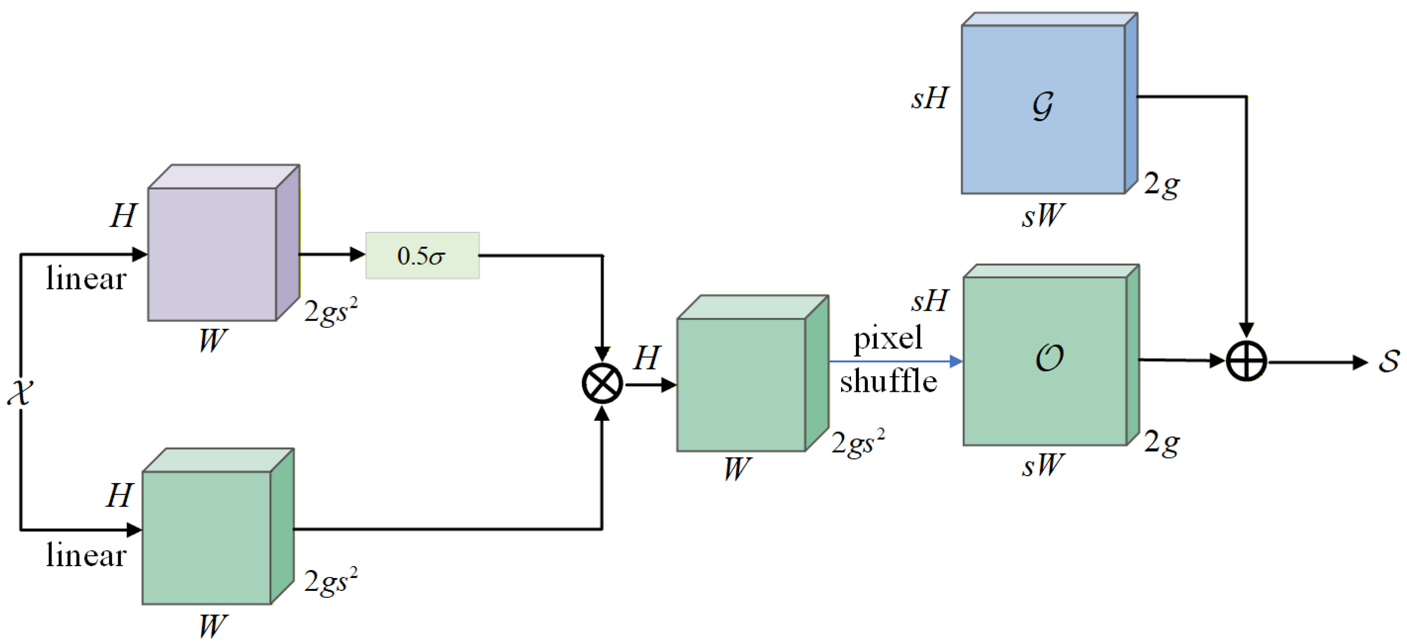
In RT-DETR, traditional bilinear interpolation is used for upsampling in both AIFI and the Hybrid Encoder. Because bilinear interpolation follows a fixed interpolation rule, it is often difficult to capture complex details in feature maps during multi-scale feature fusion, which leads to certain limitations in small-object detection tasks. Therefore, in order to improve the accuracy of small-object detection without significantly increasing the computational cost, we introduce a lightweight dynamic upsampling operator, DySample, whose structure is shown in Figure 6.

In DySample, for a feature map $\mathbf{X}$ of size $C\times H\times W$, the upsampling factor is defined as s. First, the input feature is processed by a linear layer, whose number of input channels is C and whose number of output channels is $2s^2$, thereby generating an offset tensor $\mathbf{O}$ of size $2s^2\times H\times W$. During the generation of the offsets, an additional linear layer is used to produce a dynamic range factor. Combined with the sigmoid function, this factor constrains the offset values within an appropriate range, so as to better control the offset range and ensure that sampling points do not overlap.

Then, a pixel shuffle operation is used to rearrange $\mathbf{O}$ into $2\times \left(sH\right)\times \left(sW\right)$ so that it matches the size of the target upsampled feature map. This operation adjusts the spatial distribution of the offsets, thereby ensuring that each upsampling point lies at a reasonable sampling position. Next, the generated offset $\mathbf{O}$ is added to the original grid position $\mathbf{G}$ to obtain the final sampling location set $\mathbf{S}$. Finally, the grid_sample function in PyTorch is used to sample the input feature map $\mathbf{X}$ according to the sampling location set $\mathbf{S}$, thereby generating the upsampled feature map ${\mathbf{X}}^{\prime }$. The detailed structure is shown in Figure 6. The mathematical formulation of DySample is as follows:

$$\left\{\begin{array}{cc}\hfill \mathbf{O}& =0.5\sigma \left(L1\right(\mathbf{X}\left)\right)·L2\left(\mathbf{X}\right),\hfill \\ \hfill \mathbf{S}& =\mathbf{G}+\mathbf{O},\hfill \\ \hfill {\mathbf{X}}^{\prime }& =\mathrm{grid}\_\mathrm{sample}(\mathbf{X},\mathbf{S}),\hfill \end{array}\right.$$

(1)

where $\mathbf{X}$ is the feature map of size $C\times H\times W$, $\mathbf{O}$ is the generated offset, $\mathbf{G}$ is a two-dimensional grid of size $2\times \left(sH\right)\times \left(sW\right)$ containing the original positions corresponding to all pixels during the upsampling process, and ${\mathbf{X}}^{\prime }$ is the final upsampled feature map.

Compared with the original bilinear interpolation, DySample learns the optimal sampling offset for each upsampled pixel and can automatically shift the sampling points according to image texture and semantic information, whereas bilinear interpolation relies on fixed uniform sampling and cannot effectively capture local details. Compared with other dynamic sampling operators, DySample only needs to generate two-dimensional offsets, without learning large convolution kernels or requiring high-resolution guidance features. As a result, its inference cost remains close to that of bilinear interpolation.

3.4. Convolution and Attention Fusion Module

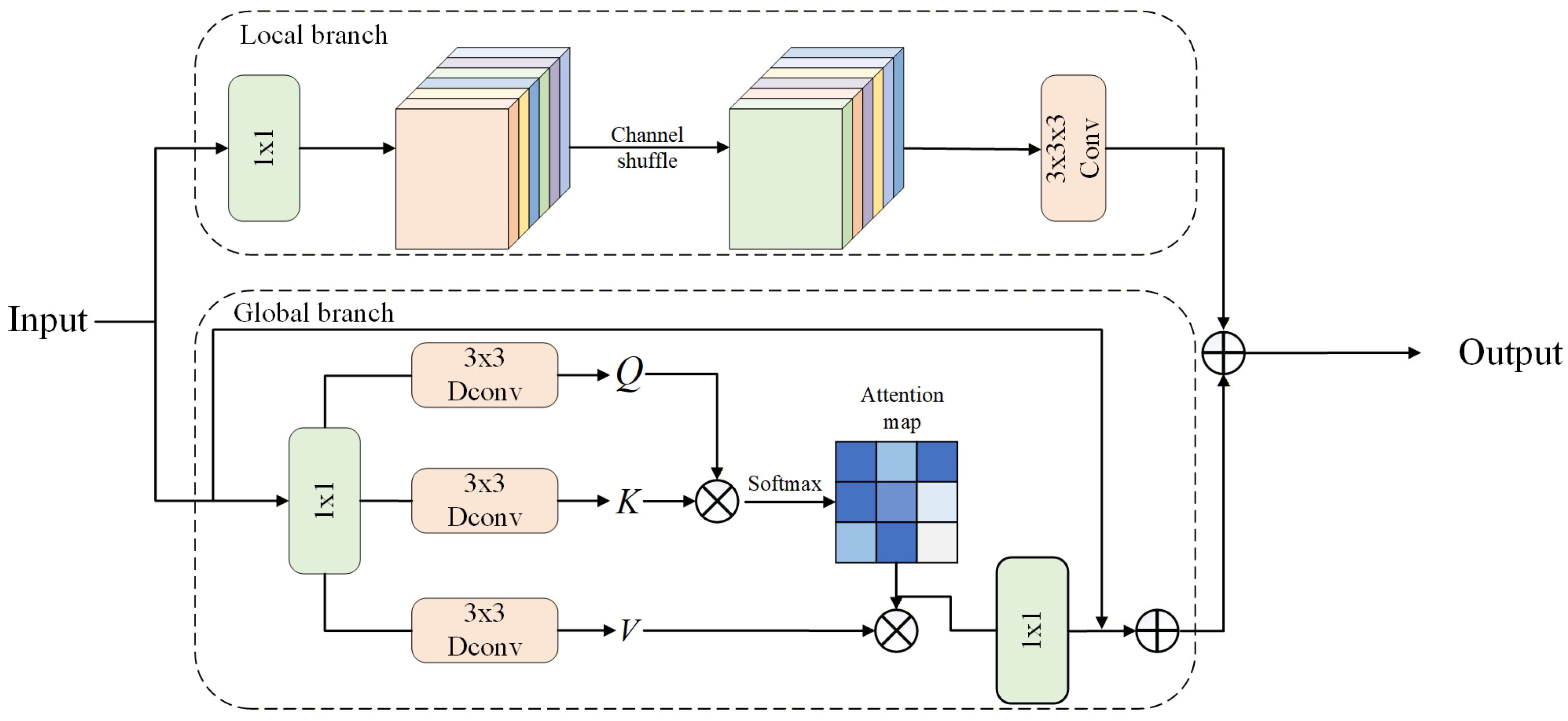
The Transformer architecture is effective at modeling global contextual features, but it is relatively weak in local feature modeling. However, in object detection tasks, the extraction of local detail features is crucial for small-object detection. Therefore, in order to enhance local feature modeling while retaining the advantage of the Transformer in global feature processing, a Convolution and Attention Fusion Module (CAFM) is introduced.

CAFM consists of two branches: a local branch and a global branch. In the local branch, the input feature $\mathbf{X}$ is first passed through a $1\times 1$ convolution to adjust the number of channels. Then, the adjusted feature ${\mathbf{X}}^{\prime }$ is divided into several groups along the channel dimension, and each group is processed independently by convolution. After the grouped convolutions, the feature channels are rearranged and inter-group information is mixed through a channel shuffle operation. Finally, a $3\times 3\times 3$ convolution is applied to extract spatial features, thereby generating the local feature representation.

In the global branch, the input feature $\mathbf{X}$ is processed by a $1\times 1$ convolution and a $3\times 3$ depthwise convolution to generate the query ($\mathbf{Q}$), key ($\mathbf{K}$), and value ($\mathbf{V}$), respectively. The attention weights (attention map) are then computed, and the global features are obtained by weighting $\mathbf{V}$ according to the attention map. The overall procedure is shown in Figure 7, and its mathematical formulation is given as follows:

$$\left\{\begin{array}{cc}\hfill {\mathbf{F}}_{\mathrm{conv}}& =W_{3\times 3\times 3}\left(\mathrm{CS}\left(W_{1\times 1}\left(\mathbf{Y}\right)\right)\right),\hfill \\ \hfill {\mathbf{F}}_{\mathrm{att}}& =W_{1\times 1}\mathrm{Attention}(\widehat{\mathbf{Q}},\widehat{\mathbf{K}},\widehat{\mathbf{V}})+\mathbf{Y},\hfill \\ \hfill \mathrm{Attention}(\widehat{\mathbf{Q}},\widehat{\mathbf{K}},\widehat{\mathbf{V}})& =\widehat{\mathbf{V}}\mathrm{Softmax}\left(\widehat{\mathbf{K}}\widehat{\mathbf{Q}}/\alpha \right),\hfill \\ \hfill {\mathbf{F}}_{\mathrm{out}}& ={\mathbf{F}}_{\mathrm{att}}+{\mathbf{F}}_{\mathrm{conv}},\hfill \end{array}\right.$$

(2)

where ${\mathbf{F}}_{\mathrm{conv}}$ denotes the output of the local branch, $W_{1\times 1}$ denotes a $1\times 1$ convolution, $\mathrm{CS}$ denotes the channel shuffle operation, $\mathbf{Y}$ denotes the input feature, and $\alpha$ is a learnable scaling parameter used to control the numerical range of the matrix multiplication result of $\widehat{\mathbf{K}}$ and $\widehat{\mathbf{Q}}$ before the Softmax function is applied.

The local branch of CAFM effectively preserves detail and texture information through channel adjustment, channel shuffle, and convolution operations. The global branch, in contrast, models long-range dependencies through the self-attention mechanism and captures the correlations of features over the global receptive field. By fusing the features from the local and global branches, CAFM achieves collaborative modeling of both local and global features.

3.5. Multiscale Feed-Forward Network

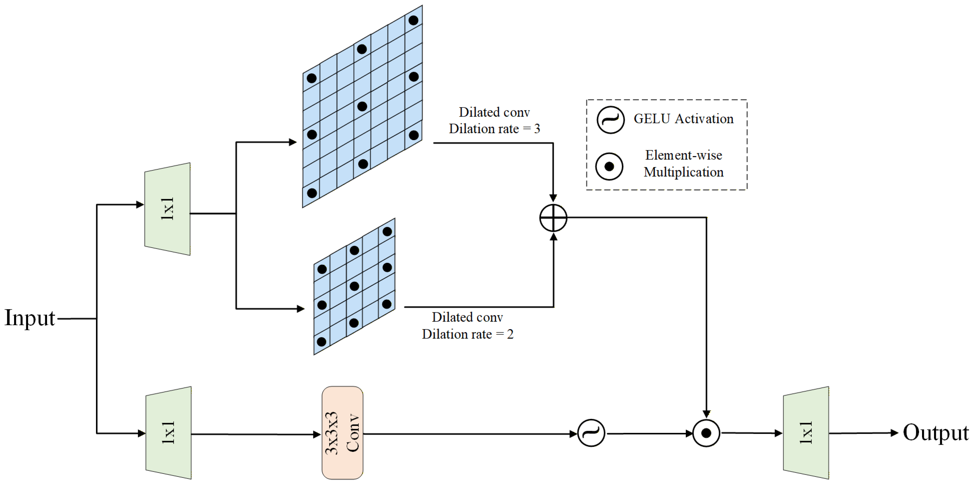
In RT-DETR, the feed-forward network (FFN) mainly consists of two fully connected layers and is used for nonlinear feature transformation. However, this single-scale feature processing manner cannot fully exploit information at different scales, which is unfavorable for small-object detection. In object detection tasks, features at different scales are of great importance. Therefore, we introduce a Multiscale Feed-Forward Network (MSFN) to enhance the multi-scale feature extraction capability of RT-DETR. Its structure is shown in Figure 8.

First, MSFN uses a $1\times 1$ convolution layer to expand the channel dimension of the input $\mathbf{X}$ from C to $2C$, generating two intermediate tensors $\mathbf{U}$ and $\mathbf{V}$. On tensor $\mathbf{U}$, MSFN performs two parallel $3\times 3$ dilated convolutions, with dilation rates of 2 and 3, respectively. The two outputs are then added element-wise along the channel dimension to form the output ${\mathbf{U}}^{\prime }$. Meanwhile, tensor $\mathbf{V}$ is processed by a $3\times 3$ depthwise separable convolution, followed by the GELU activation function, to obtain the output ${\mathbf{V}}^{\prime }$. Subsequently, ${\mathbf{U}}^{\prime }$ and ${\mathbf{V}}^{\prime }$ are multiplied element-wise through a gating operation. Finally, the gated tensor is projected back to the original channel dimension C through a $1\times 1$ convolution, producing the final output ${\mathbf{X}}_{\mathrm{out}}$ of MSFN. Its mathematical formulation is given as follows:

$$\left\{\begin{array}{cc}\hfill {\mathbf{U}}^{\prime }& =\left(W_{3\times 3}^2{W}_{1\times 1}\left(\mathbf{X}\right)+W_{3\times 3}^3{W}_{1\times 1}\left(\mathbf{X}\right)\right),\hfill \\ \hfill {\mathbf{V}}^{\prime }& =\varphi \left(W_{3\times 3}{W}_{1\times 1}\left(\mathbf{X}\right)\right),\hfill \\ \hfill \mathrm{Gating}\left(\mathbf{X}\right)& ={\mathbf{U}}^{\prime }\odot {\mathbf{V}}^{\prime },\hfill \\ \hfill {\mathbf{X}}_{\mathrm{out}}& =W_{1\times 1}\mathrm{Gating}\left(\mathbf{X}\right),\hfill \end{array}\right.$$

(3)

where ⊙ denotes element-wise multiplication, $\varphi$ denotes the GELU nonlinear activation function, $W_{3\times 3}^2$ denotes the $3\times 3$ dilated convolution with dilation rate 2, and $W_{3\times 3}^3$ denotes the $3\times 3$ dilated convolution with dilation rate 3.

Dilated convolution can significantly enlarge the receptive field without increasing the kernel size. In one branch of MSFN, the two parallel $3\times 3$ dilated convolutions, with dilation rates of 2 and 3, capture medium-scale and large-scale spatial contextual information, respectively. In this way, the network can not only focus on the detailed features of small objects, but also obtain the global semantic information of their surrounding background, thereby improving the discriminability of small objects in complex scenes. In the other branch, depthwise separable convolution combined with GELU activation is adopted to extract finer local features and enhance nonlinear representation capability. Finally, through the gating mechanism based on element-wise multiplication, the outputs of the two branches are fused, so that only the features that are simultaneously emphasized in multi-scale context and local details are retained, whereas noise and redundant information are automatically suppressed. As a result, the detection performance for small objects that are easily overwhelmed by background noise is substantially improved.

3.6. Marker-Based Posture Recognition Method

3.6.1. Marker Installation Design

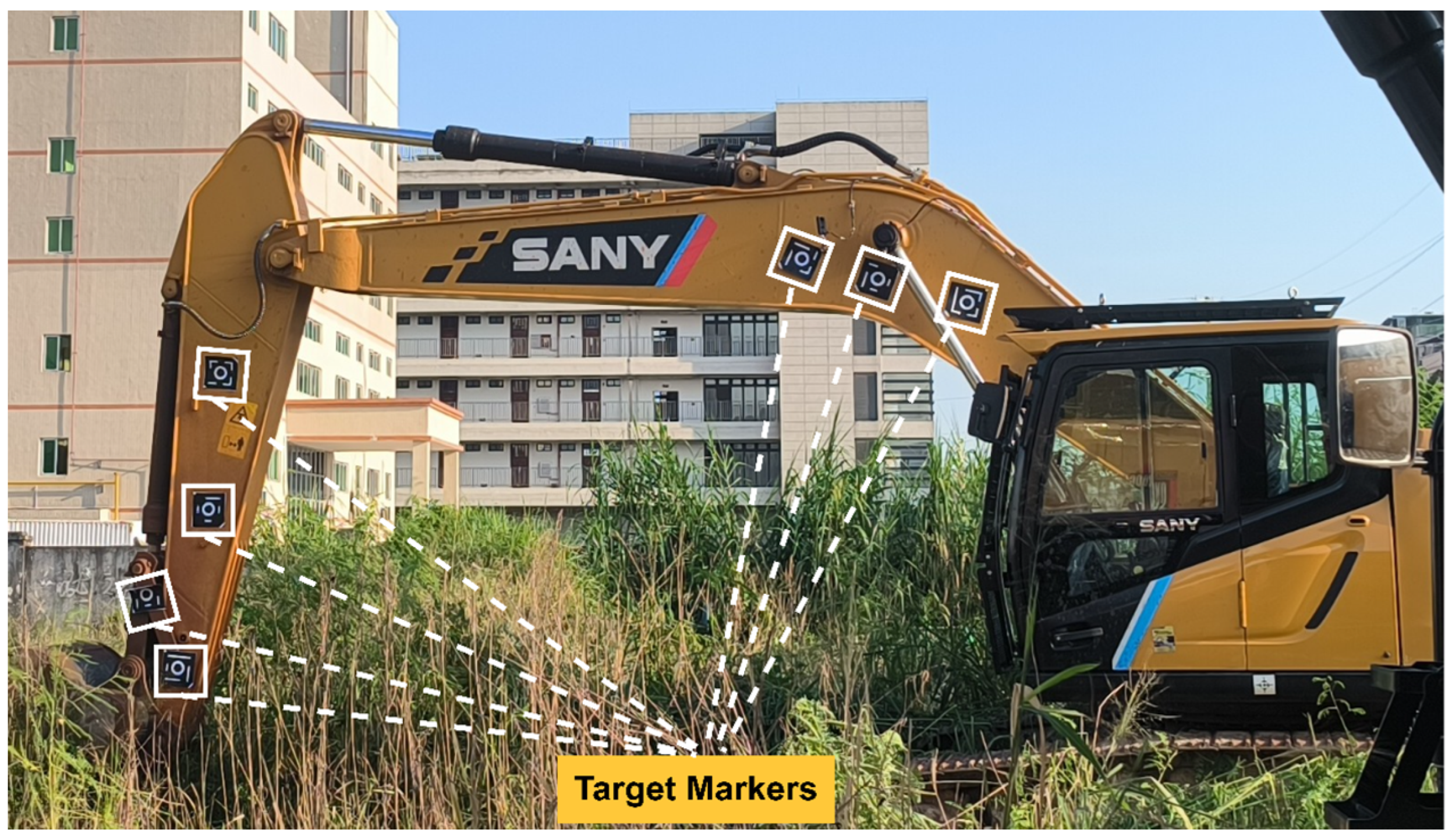
Three markers are mounted on the boom, two on the stick, and two at the articulation point between the stick and the bucket. The line connecting the centers of the markers is arranged to be parallel to the principal span of the corresponding component. In general, two markers are insufficient to accurately represent posture. Because the boom has a relatively large span, three markers are installed on it to achieve more accurate posture representation and to facilitate subsequent processing. The overall installation design is shown in Figure 9.

3.6.2. Kinematic Modeling Based on the D–H Method

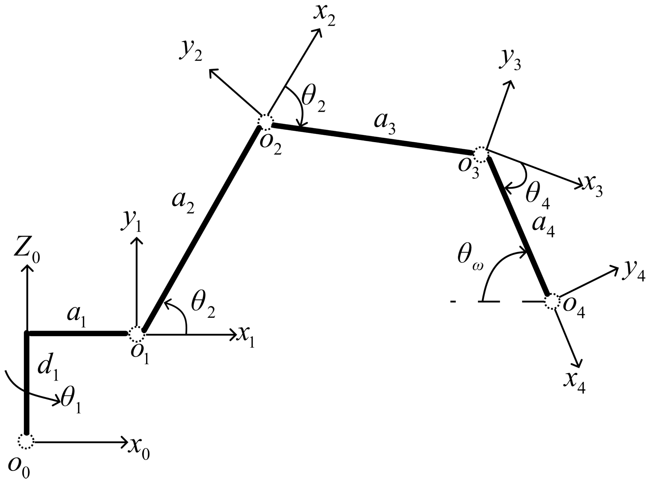
As shown in Figure 10, the link coordinate system of the excavator working device is established using the Denavit–Hartenberg (D–H) method. The base coordinate system is denoted as $x_0{y}_0{z}_0{o}_0$, while the coordinate systems of the boom, stick, bucket, and bucket tip are denoted as $x_1{y}_1{z}_1{o}_1$, $x_2{y}_2{z}_2{o}_2$, $x_3{y}_3{z}_3{o}_3$, and $x_4{y}_4{z}_4{o}_4$, respectively. In the figure, the z-axis is aligned with the rotation axis of each joint, whereas the coordinate axis perpendicular to the paper plane is omitted. The joint space of the excavator is composed of four joint angle variables: the swing joint ${\theta }_1$, boom joint ${\theta }_2$, stick joint ${\theta }_3$, and bucket joint ${\theta }_4$. The pose space is determined by the three-dimensional position $[x,y,z]$ of the bucket tip in the base coordinate system $x_0{y}_0{z}_0{o}_0$ and the orientation angle ${\theta }_{\omega }$. Assuming that the counterclockwise direction is positive for each joint angle, according to Ref. [27], the transformation from the coordinate system $x_{i-1}{y}_{i-1}{z}_{i-1}{o}_{i-1}$ to $x_i{y}_i{z}_i{o}_i$ can be expressed in matrix form as follows:

$$T_{i-1}^i=\left(\begin{array}{cccc}{C}_i& -cos{\alpha }_i{S}_i& sin{\alpha }_i{S}_i& a_i{C}_i\\ S_i& cos{\alpha }_i{C}_i& -sin{\alpha }_i{C}_i& a_i{S}_i\\ 0& sin{\alpha }_i& cos{\alpha }_i& d_i\\ 0& 0& 0& 1\end{array}\right)$$

(4)

where $C_i$ denotes $cos{\theta }_i$, $S_i$ denotes $sin{\theta }_i$, ${\alpha }_i$ is the link twist angle, $a_i$ is the link length, and $d_i$ is the link offset.

The transformation from $x_0{y}_0{z}_0{o}_0$ to $x_4{y}_4{z}_4{o}_4$ can therefore be written as

$$T_0^4=T_0^1{T}_1^2{T}_2^3{T}_3^4=\left(\begin{array}{cccc}{C}_1{C}_{234}& -C_1{S}_{234}& S_1& C_1(a_4{C}_{234}+a_3{C}_{23}+a_2{C}_2+a_1)\\ S_1{C}_{234}& -S_1{S}_{234}& -C_1& S_1(a_4{C}_{234}+a_3{C}_{23}+a_2{C}_2+a_1)\\ S_{234}& C_{234}& 0& a_4{S}_{234}+a_3{S}_{23}+a_2{S}_2+d_1\\ 0& 0& 0& 1\end{array}\right).$$

(5)

Here, $S_i$, $C_i$, $S_{ij}$, and $C_{ij}$ denote $sin{\theta }_i$, $cos{\theta }_i$, $sin({\theta }_i+{\theta }_j)$, and $cos({\theta }_i+{\theta }_j)$, respectively.

According to the above equation, the following expressions can be obtained:

$$\left\{\begin{array}{cc}\hfill x& =C_1(a_4{C}_{234}+a_3{C}_{23}+a_2{C}_2+a_1),\hfill \\ \hfill y& =S_1(a_4{C}_{234}+a_3{C}_{23}+a_2{C}_2+a_1),\hfill \\ \hfill z& =a_4{S}_{234}+a_3{S}_{23}+a_2{S}_2+d_1,\hfill \\ \hfill {\theta }_{\omega }& ={\theta }_2+{\theta }_3+{\theta }_4.\hfill \end{array}\right.$$

(6)

where ${\theta }_{\omega }$ denotes the orientation angle of the end effector (bucket tip).

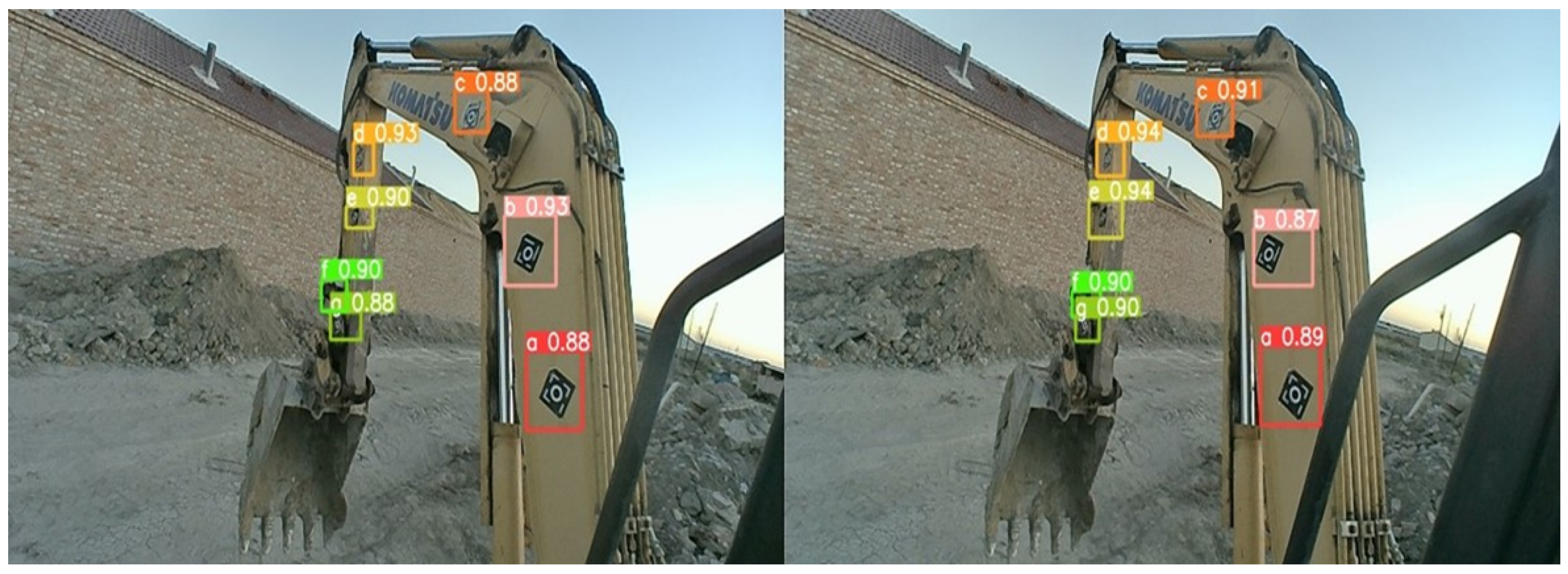
3.6.3. Posture Angle Calculation

The improved RT-DETR framework is first used to detect the target, as shown in Figure 11. Then, the ZED camera is used to obtain the three-dimensional point-cloud coordinates corresponding to the center point of the target [28,29,30]. For clarity, the 3D coordinate of a detected marker center in the camera frame is denoted by ${\mathbf{p}}^c={(x^c,y^c,z^c)}^{\top }$, whereas its coordinate in the world frame is denoted by ${\mathbf{p}}^w={(X,Y,Z)}^{\top }$. In addition, the symbols ${\theta }_1$, ${\theta }_2$, ${\theta }_3$, and ${\theta }_4$ are reserved for the D–H joint variables defined above, while the marker-based posture angles of the boom, stick, bucket linkage, and bucket are denoted by ${\beta }_{\mathrm{boom}}$, ${\beta }_{\mathrm{stick}}$, ${\beta }_{\mathrm{link}}$, and ${\beta }_{\mathrm{bucket}}$, respectively. The 3D point-cloud coordinates acquired by the ZED camera must then be transformed into world coordinates. In the ZED 3D point-cloud coordinate system, the positive x-axis points to the right side of the camera, the positive y-axis points upward (toward the sky), and the positive z-axis points backward from the camera. Therefore, a coordinate transformation is required, such that the z-axis in the 3D point-cloud coordinate system corresponds to the Y-axis in the real-world coordinate system, the x-axis corresponds to the X-axis in the real-world coordinate system, and the y-axis corresponds to the Z-axis in the real-world coordinate system. Assuming that the camera height is $Z_D$, and that the camera is fixed parallel to the ground plane, the corresponding world coordinate can be expressed as

$$X=x^c,Y=z^c,Z=y^c-Z_D.$$

(7)

According to Equation (7), the world coordinate of each marker center can be written as ${\mathbf{p}}^w={(X,Y,Z)}^{\top }$.

For the three boom markers a, b, and c, let their world coordinates be ${\mathbf{p}}_a={(X_a,Y_a,Z_a)}^{\top }$, ${\mathbf{p}}_b={(X_b,Y_b,Z_b)}^{\top }$, and ${\mathbf{p}}_c={(X_c,Y_c,Z_c)}^{\top }$, respectively. Define the three direction vectors

$${\mathbf{v}}_{ab}={\mathbf{p}}_b-{\mathbf{p}}_a,{\mathbf{v}}_{ac}={\mathbf{p}}_c-{\mathbf{p}}_a,{\mathbf{v}}_{bc}={\mathbf{p}}_c-{\mathbf{p}}_b.$$

(8)

Let the normal vector of the ground plane be ${\mathbf{n}}_g={(0,0,1)}^{\top }$. Then, the absolute angles between the three marker-connection lines and the ground plane are defined as

$$\left\{\begin{array}{cc}\hfill {\alpha }_{ab}& =arcsin\left({\displaystyle \frac{|{\mathbf{v}}_{ab}·{\mathbf{n}}_g|}{\parallel {\mathbf{v}}_{ab}\parallel }}\right),\hfill \\ \hfill {\alpha }_{ac}& =arcsin\left({\displaystyle \frac{|{\mathbf{v}}_{ac}·{\mathbf{n}}_g|}{\parallel {\mathbf{v}}_{ac}\parallel }}\right),\hfill \\ \hfill {\alpha }_{bc}& =arcsin\left({\displaystyle \frac{|{\mathbf{v}}_{bc}·{\mathbf{n}}_g|}{\parallel {\mathbf{v}}_{bc}\parallel }}\right).\hfill \end{array}\right.$$

(9)

The boom posture angle is then obtained by averaging the three estimates, i.e.,

$${\beta }_{\mathrm{boom}}={\displaystyle \frac{{\alpha }_{ab}+{\alpha }_{ac}+{\alpha }_{bc}}{3}}.$$

(10)

For the boom and stick, according to the coded-marker layout shown in Figure 9, the line connecting the coded markers is parallel to the line of the corresponding component itself. Therefore, the obtained inclination angle can be directly used as the posture angle of that component. In particular, the stick posture angle ${\beta }_{\mathrm{stick}}$ is obtained from the inclination angle of the connecting vector between its two corresponding markers using the same definition as in Equation (9). Similarly, the posture angle of the bucket linkage is first estimated from the coded markers mounted on linkage $AB$ and is denoted by ${\beta }_{\mathrm{link}}$. Since the bucket is often buried in soil during operation, the coded markers are attached to the bucket linkage rather than the bucket itself, and the final bucket posture angle is then obtained through geometric transformation.

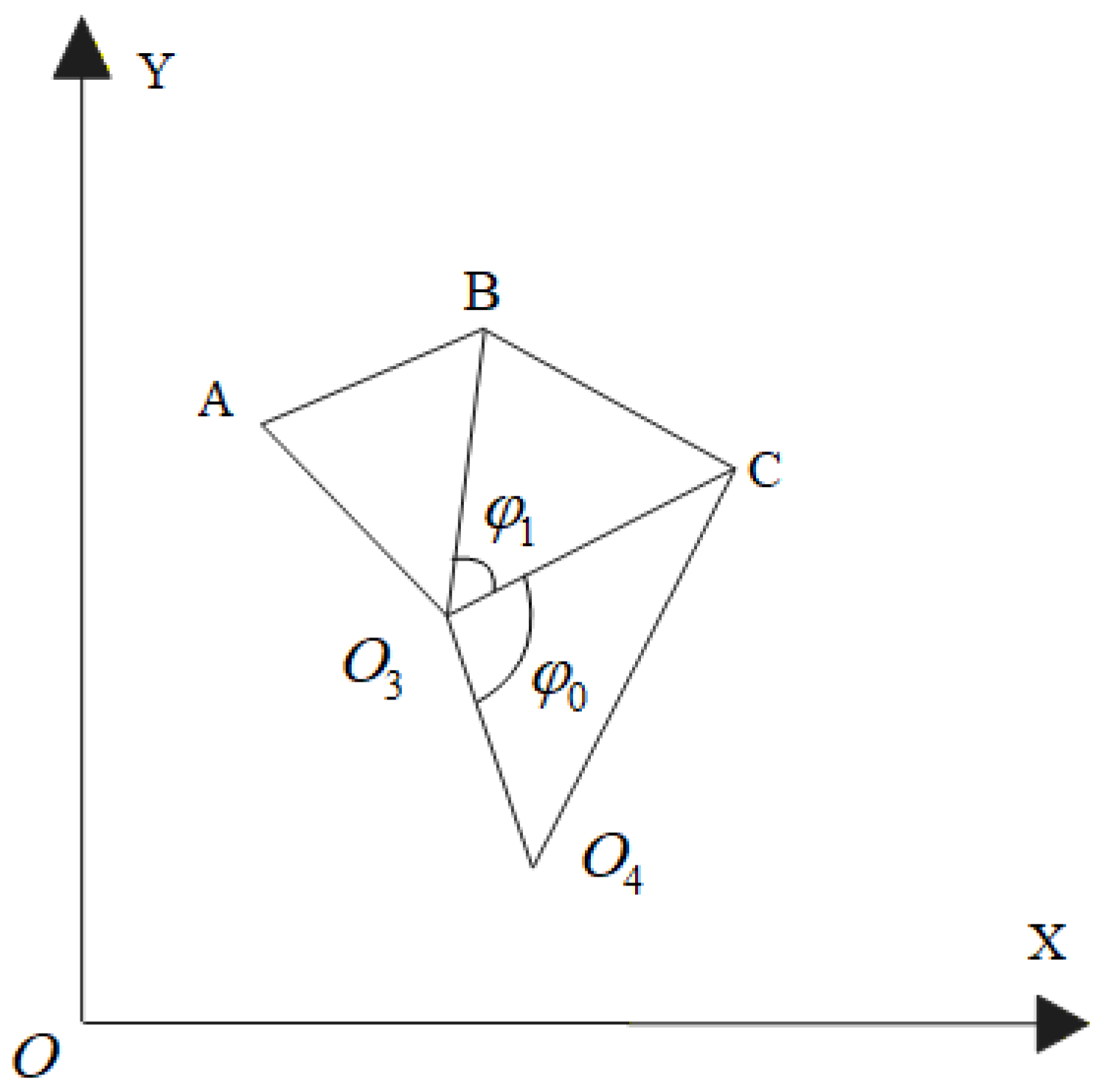
Figure 12 shows a schematic diagram of the structure of the stick, bucket, and additional linkage. In $O_3{O}_{4}C$, the hinge point connected to the stick is $O_3$, and the bucket tip is $O_4$, while $O_{3}A$ is located on the stick. The coded markers are attached to linkage $AB$, and the other linkage is $BC$. Let ${\mathbf{r}}_{O_{3}B}$ denote the vector from $O_3$ to B. Then,

$${\mathbf{r}}_{O_{3}B}={\mathbf{r}}_{AB}-{\mathbf{r}}_{A{O}_3}.$$

Let ${\varphi }_2$ denote the orientation angle of ${\mathbf{r}}_{O_{3}B}$ in the working plane. Then,

$${\varphi }_2=atan2\left(|{\mathbf{r}}_{AB}|sin{\beta }_{\mathrm{link}}-|{\mathbf{r}}_{A{O}_3}|sin({\theta }_2+{\theta }_3),|{\mathbf{r}}_{AB}|cos{\beta }_{\mathrm{link}}-\left|{\mathbf{r}}_{A{O}_3}\right|cos({\theta }_2+{\theta }_3)\right),$$

(11)

where

$${\mathbf{r}}_{AB}=\left(|{\mathbf{r}}_{AB}|cos{\beta }_{\mathrm{link}},\left|{\mathbf{r}}_{AB}\right|sin{\beta }_{\mathrm{link}}\right),{\mathbf{r}}_{A{O}_3}=\left(|{\mathbf{r}}_{A{O}_3}|cos({\theta }_2+{\theta }_3),\left|{\mathbf{r}}_{A{O}_3}\right|sin({\theta }_2+{\theta }_3)\right).$$

The auxiliary angle ${\varphi }_1$ is given by

$${\varphi }_1=arccos\left({\displaystyle \frac{|O_3{B|}^2+|O_3{C|}^2-{\left|BC\right|}^2}{2|O_{3}C\left|\right|BC|}}\right),$$

(12)

where ${\varphi }_0$ is a constant structural offset angle determined by the bucket-linkage geometry. Therefore, the bucket posture angle is

$${\beta }_{\mathrm{bucket}}={\varphi }_2-{\varphi }_1-{\varphi }_0.$$

(13)

The final posture estimation is affected by multiple geometric uncertainty sources, including stereo-camera calibration error, depth noise in 3D point recovery, and inaccuracies in the camera-to-world coordinate transformation. In the proposed pipeline, these uncertainties mainly influence the reconstructed 3D coordinates of the marker centers and then propagate to the subsequent angle computation. Nevertheless, because the boom and stick angles are estimated from the relative geometric relationships among multiple markers on the same component, common translational perturbations can be partially canceled. In addition, the boom angle is obtained by averaging multiple marker-based estimates, which further improves robustness against random 3D perturbations.

4. Results

4.1. Experimental Environment and Dataset

The experiments were conducted on a 64-bit Ubuntu 22.04 platform equipped with an NVIDIA GeForce RTX 4090 GPU (24 GB). The model was implemented using PyTorch 2.0.1, and data were collected with a ZED2i stereo camera. In addition, contact sensors were installed on the excavator to measure the posture angles of the working device, and the dataset also includes the angle data returned by these contact sensors. The complete raw dataset consisted of 45,391 annotated images extracted from 30 video sequences. A total of seven coded-marker categories were annotated, denoted as Marker-a to Marker-g, corresponding to the seven physical markers mounted on the boom, stick, and bucket linkage shown in Figure 9. During image annotation, the bounding boxes of the seven coded markers were manually labeled on the extracted image frames, and each bounding box was assigned to its corresponding marker category. The ground-truth posture angles were obtained from the synchronized measurements of the contact sensors mounted on the excavator during data acquisition. The sensor readings were aligned with the image frames through timestamp synchronization and were used as reference values for the subsequent posture-angle evaluation. In addition, because one image may contain multiple markers, the class distribution is reported in terms of labeled instances rather than images. The numbers of labeled instances for Marker-a to Marker-g were 39,110, 38,699, 37,295, 35,690, 35,225, 33,625, and 33,056, respectively.

To avoid data leakage, the dataset was partitioned at the video-sequence level before data augmentation; therefore, images from the same video sequence were assigned exclusively to one subset. Specifically, the training, validation, and test sets contained 36,313, 4539, and 4539 raw images, respectively, corresponding to 24, 3, and 3 video sequences. Random data augmentation operations, including flipping and translation, were applied only to the training set during model training. The detailed numbers of labeled instances for each marker category in the three subsets are summarized in

Table 1. Detailed statistics of the excavator marker dataset.

Marker Category	Train	Validation	Test	Total
Marker-a	31,274	3944	3892	39,110
Marker-b	30,981	3812	3906	38,699
Marker-c	29,847	3706	3742	37,295
Marker-d	28,596	3517	3577	35,690
Marker-e	28,214	3463	3548	35,225
Marker-f	26,928	3305	3392	33,625
Marker-g	26,511	3244	3301	33,056
Raw images	36,313	4539	4539	45,391
Video sequences	24	3	3	30

.

4.2. Evaluation Metrics

In this study, Recall, mean average precision (mAP), and the number of parameters (Parameters) were used as the evaluation metrics. The mAP is obtained by first calculating the average precision (AP) for each object category and then averaging the AP values over all categories. In the precision–recall (P–R) curve, precision (P) is plotted on the vertical axis and recall (R) on the horizontal axis, and the area under the curve corresponds to the AP. For multi-class tasks, the AP values of all categories are summed and then divided by the number of categories to obtain the mAP. The formulas are given as follows:

$$R={\displaystyle \frac{TP}{TP+FN}}$$

(14)

$$\mathrm{mAP}={\displaystyle \frac{1}{n}}\sum _{i=1}^{n}A{P}_i$$

(15)

where $TP$ denotes the number of true positive samples, $FP$ denotes the number of false positive samples, and $FN$ denotes the number of false negative samples. Here, n is the total number of object categories. The AP is defined as the integral of precision over the recall interval from 0 to 1:

$$AP={\int }_0^{1}p\left(r\right)dr$$

(16)

where $p\left(r\right)$ denotes precision as a function of recall, i.e.,

$$p\left(r\right)={\displaystyle \frac{TP}{TP+FP}}.$$

(17)

In addition to object-detection performance, the final posture-angle estimation accuracy of the proposed pipeline was evaluated against the synchronized readings of the contact sensors. For each component $j\in \{\mathrm{boom},\mathrm{stick},\mathrm{bucket}\}$, the mean absolute error (MAE) and root mean square error (RMSE) were calculated in degrees as follows:

$${\mathrm{MAE}}_j={\displaystyle \frac{1}{N}}\sum _{i=1}^N\left|{\widehat{\theta }}_{j,i}-{\theta }_{j,i}^{\mathrm{ref}}\right|$$

(18)

$${\mathrm{RMSE}}_j=\sqrt{{\displaystyle \frac{1}{N}}\sum _{i=1}^N{\left({\widehat{\theta }}_{j,i}-{\theta }_{j,i}^{\mathrm{ref}}\right)}^2}$$

(19)

where ${\widehat{\theta }}_{j,i}$ and ${\theta }_{j,i}^{\mathrm{ref}}$ denote the predicted angle and the reference angle measured by the contact sensor for the ith sample, respectively.

4.3. Model Comparison

To verify the superiority and effectiveness of the proposed improved model, comparative experiments were conducted. The proposed method was compared with YOLO-series models, DETR-series models, and a fully convolutional network, and the results are presented in

Table 2. Comparison results of different object detection models.

Model	Recall/%	mAP/%	Parameters (M)
YOLOv5m	85.23	84.56	25.1
YOLOv8m	86.34	85.67	25.9
YOLOv11m	87.41	81.54	20.1
DETR	82.14	85.75	43.6
Deformable-DETR	81.65	81.56	35.2
RT-DETR	88.19	86.33	28.9
FCN	83.15	84.34	23.7
RevCol-S	87.24	89.25	28.2
FocalNet-S	89.23	91.24	61.3
Ours	93.57	94.29	18.8

. Meanwhile, to ensure the fairness of the comparison, all detector models listed in Table 2 were trained and evaluated under a unified experimental setting. Specifically, all models used the same training/validation/test split, the same input image resolution of 640 × 640, and the same data augmentation strategy, including random flipping and translation. Except for architecture-specific components that are inherently required by each model, the optimizer settings and learning rate scheduling strategy were kept consistent across all models.

As shown in Table 2, the proposed method achieves the best overall performance among all compared models. Recall and mAP are the primary metrics for evaluating detection accuracy, whereas the number of parameters reflects model complexity and computational cost. In terms of detection accuracy, the proposed method attains a Recall of 93.57% and an mAP of 94.29%, which are higher than those of all the compared models. Compared with the baseline RT-DETR, Recall and mAP are improved by 5.38% and 7.96%, respectively, demonstrating that the proposed improvements significantly enhance detection performance. Compared with YOLOv5m, the proposed method improves Recall by 8.34% and mAP by 9.73%. In comparison with recently introduced models such as RevCol-S and FocalNet-S, the proposed method still achieves higher Recall and mAP while maintaining a substantially lower number of parameters, especially when compared with FocalNet-S. In terms of computational efficiency, the proposed model contains only 18.8M parameters, which is fewer than all the other compared models in Table 2. These results indicate that the proposed method provides a better trade-off between detection accuracy and model complexity and is more suitable for practical deployment in resource-constrained environments.

4.4. Comparison of Backbone Designs

To verify the rationality of using RepViT, several lightweight backbone networks, including RepViT, EfficientViT, and StarNet, were selected for comparison. By comparing the AP values of each target category as well as the overall mAP, the most suitable backbone for replacing the original backbone in RT-DETR was determined.

As shown in

Table 3. Comparison results of different backbone replacements.

Model	APa	APb	APc	APd	APe	APf	APg	mAP/%	Params (M)
RT-DETR	81.83	81.83	84.57	86.60	87.43	90.26	92.13	86.33	28.9
RT-DETR + RepViT	82.75	82.54	84.75	88.35	90.44	94.04	92.77	88.78	14.2
RT-DETR + LSKNet	84.79	81.37	80.16	85.85	94.25	93.58	94.26	87.75	17.7
RT-DETR + EfficientViT	82.82	84.16	85.30	86.96	86.83	88.75	89.30	86.30	11.8
RT-DETR + EMO	82.73	82.33	86.64	86.01	88.39	87.87	86.80	85.82	12.4
RT-DETR + VanillaNet	83.49	80.32	80.37	89.24	89.69	93.05	83.29	87.02	19.8
RT-DETR + StarNet	84.10	82.27	86.30	86.49	94.15	89.82	94.26	88.20	16.9

, after introducing lightweight backbone networks such as RepViT, EfficientViT, and StarNet, the mAP of the model is improved to varying degrees. Specifically, replacing the original backbone with RepViT improves the mAP by 2.45%, whereas replacing it with StarNet improves the mAP by 1.87%. Among all compared backbones, RepViT achieves the largest improvement in mAP. Although the mAP improvement of StarNet is close to that of RepViT, its number of parameters is 2.7 M higher than that of RepViT. Therefore, considering both performance and parameter efficiency, RepViT is finally selected as the backbone of RT-DETR.

4.5. Comparison of Upsampling Operators

To better exploit multi-scale features, the bilinear interpolation used in RT-DETR was replaced with dynamic upsampling operators. In order to identify the most suitable upsampling operator, different dynamic upsampling methods were employed to replace bilinear interpolation, and their parameter increments and mAP values were compared. Based on these results, the optimal upsampling operator was selected.

As shown in

Table 4. Comparison results of different upsampling operators.

Model	APa	APb	APc	APd	APe	APf	APg	mAP/%	Params (M)
RT-DETR (RepViT)	82.75	82.54	84.75	88.35	90.44	94.04	92.77	88.78	14.2
+ DySample	87.35	89.77	91.75	91.56	92.67	91.42	93.03	91.03	15.3
+ CARAFE	81.34	88.10	87.81	89.35	92.63	93.91	94.89	89.72	16.2
+ SAPA	87.59	83.20	90.89	88.13	90.99	92.27	92.61	89.38	15.7
+ Transposed Convolution	84.46	87.63	88.48	88.86	89.54	90.33	93.10	90.91	17.8

, after introducing different upsampling operators, the mAP of the model is significantly improved. Specifically, replacing bilinear interpolation with DySample improves the mAP by 2.25%, whereas using transposed convolution improves the mAP by 2.13%. Although the mAP improvement achieved by transposed convolution is close to that of DySample, DySample yields the largest overall performance gain, while requiring 1.5 M fewer parameters than SAPA. Therefore, considering both performance improvement and parameter efficiency, DySample is ultimately selected as the optimal upsampling operator.

4.6. Ablation Study

To verify the effectiveness of the proposed improvement strategies, ablation experiments were conducted based on the baseline RT-DETR model, and the performance of small-object detection was evaluated on the validation set. The experimental results are presented in

Table 5. Results of the ablation study.

Model	APa	APb	APc	APd	APe	APf	APg	mAP/%
RT-DETR	81.91	81.88	84.63	86.68	87.52	90.31	91.94	86.41 ± 0.22
RT-DETR + RepViT	83.44	83.12	85.58	89.17	91.46	94.78	94.47	88.86 ± 0.19
RT-DETR + RepViT + DySample	87.46	89.92	91.81	91.68	92.79	91.54	92.57	91.11 ± 0.16
RT-DETR + RepViT + DySample + CAFM	92.26	89.08	93.04	94.18	93.62	94.44	94.24	92.98 ± 0.14
RT-DETR + RepViT + DySample + CAFM + MSFN	94.95	94.16	93.62	93.58	95.47	95.02	93.72	94.36 ± 0.12

and

Table 6. Results of the Ablation Study on Changes in Parameters and GFLOPs.

Model	$\mathbf{\Delta }$mAP/%	Params (M)	$\mathbf{\Delta }$Params (M)	GFLOPs	$\mathbf{\Delta }$GFLOPs
RT-DETR	–	28.9	–	96.8	–
RT-DETR + RepViT	+2.45	14.2	-14.7	55.4	-41.4
RT-DETR + RepViT + DySample	+2.25	15.3	+1.1	58.1	+2.7
RT-DETR + RepViT + DySample + CAFM	+1.87	16.9	+1.6	64.7	+6.6
RT-DETR + RepViT + DySample + CAFM + MSFN	+1.38	18.8	+1.9	72.3	+7.6

. The proposed model mainly includes the following four improvements: a lightweight backbone based on RepViT, the DySample-based upsampling optimization, CAFM, and MSFN.

Table 5 and Table 6 further show that, after rerunning the ablation experiments, replacing the backbone of RT-DETR with RepViT improves the mean mAP from 86.41% to 88.86%, i.e., by 2.45%, while reducing the parameter count from 28.9 M to 14.2 M and the computational complexity from 96.8 GFLOPs to 55.4 GFLOPs. This confirms that RepViT is the main source of lightweight improvement in the proposed model. On this basis, replacing bilinear interpolation with DySample further improves the mean mAP by 2.25% with only a small overhead of 1.1 M parameters and 2.7 GFLOPs, indicating a favorable accuracy–complexity trade-off. After introducing CAFM, the mean mAP is further increased by 1.87%, while the parameter count and computational complexity rise moderately by 1.6 M and 6.6 GFLOPs, respectively. Finally, after replacing the FFN with MSFN, the mean mAP is further improved by 1.38%, with an additional overhead of 1.9 M parameters and 7.6 GFLOPs. In addition, the standard deviation of mAP over three independent runs remains small, decreasing from 0.22 to 0.12. The updated class-wise AP values and the small run-to-run variations jointly indicate that the gains introduced by RepViT, DySample, CAFM, and MSFN are stable rather than incidental.

The updated ablation results indicate that the lightweight backbone based on RepViT, the advanced dynamic upsampling operator, and the sufficient utilization of multi-scale features consistently improve the performance of small-object detection while maintaining stable gains over repeated runs.

4.7. Edge Deployment Evaluation on Jetson Orin NX 8GB

To further evaluate the deployment capability of the proposed method in resource-constrained scenarios, additional experiments were conducted on the NVIDIA Jetson Orin NX 8GB platform. As a representative embedded edge computing device, the Jetson Orin NX 8GB provides significantly lower computational power and memory resources than desktop GPUs such as the NVIDIA GeForce RTX 4090. Therefore, experiments on this platform can better demonstrate the practicality and feasibility of the proposed method for edge deployment.

Under TensorRT FP16 inference with an input size of 320 × 320,

Table 7. Deployment performance of different models on the Jetson Orin NX 8GB platform.

Model	Params (M)	Peak Memory (GB)	Latency (ms)	FPS
YOLOv5m	25.1	1.24	28	36
YOLOv8m	25.9	1.28	25	40
YOLOv11m	20.1	1.16	22	45
DETR	43.6	2.11	71	14
Deformable-DETR	35.2	1.87	52	19
RT-DETR	28.9	1.61	39	26
FCN	23.7	1.36	34	29
RevCol-S	28.2	1.55	36	28
FocalNet-S	61.3	2.74	105	10
Ours	18.8	1.33	29	34

presents the performance of different models on the Jetson Orin NX 8GB platform. YOLOv11m achieves the lowest inference latency of 22 ms (45 FPS), whereas the proposed method attains a latency of 29 ms (34 FPS), which is only slightly higher than that of the lightweight YOLO models, while using the smallest number of parameters, i.e., only 18.8 M. In contrast, transformer-based models such as DETR, Deformable-DETR, and RT-DETR exhibit higher latency, reaching 71 ms, 52 ms, and 39 ms, respectively. FocalNet-S incurs the highest deployment cost, with a latency of 105 ms and a peak memory usage of 2.74 GB. Overall, the proposed method achieves a favorable balance among accuracy, latency, FPS, parameter size, and memory usage, making it more suitable for deployment in resource-constrained edge scenarios.

4.8. Pose Estimation Accuracy Analysis

To quantitatively evaluate the final posture-estimation accuracy of the proposed method, the predicted boom, stick, and bucket angles on the test set were compared with the synchronized measurements obtained from the contact sensors. It should be noted that the reported MAE and RMSE are end-to-end errors of the complete pipeline and therefore implicitly include the cumulative effects of multiple error sources, including marker-detection uncertainty, stereo depth noise, camera calibration error, and world-coordinate transformation error. The relatively larger error observed for the bucket angle is also consistent with the fact that it is obtained through an additional linkage-based geometric transformation, which makes it more sensitive to upstream 3D coordinate perturbations.

Table 8. Quantitative accuracy of excavator posture-angle estimation on the test set.

Component	MAE (°)	RMSE (°)
Boom	1.18	1.56
Stick	1.43	1.87
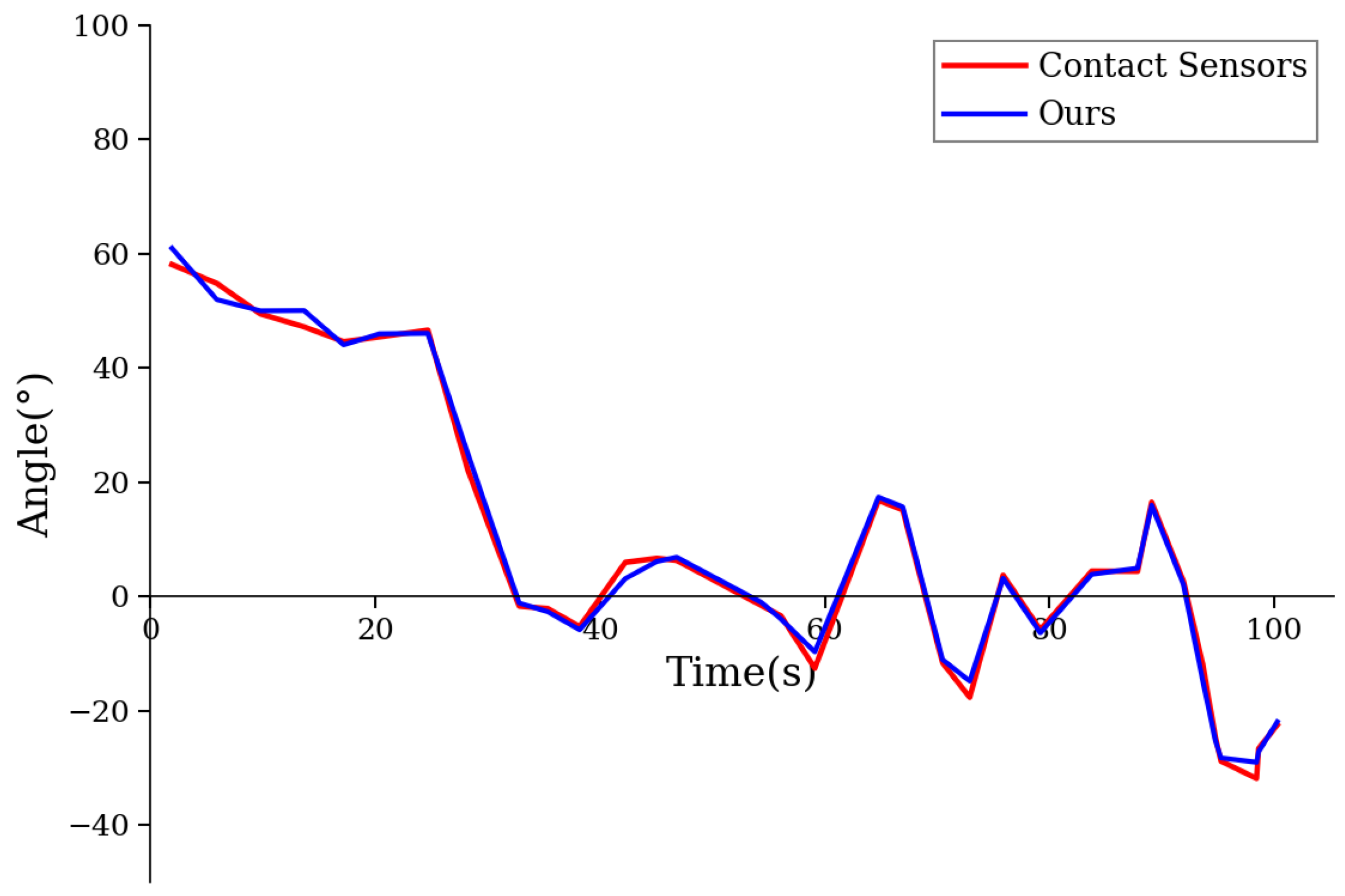
Bucket	2.06	2.71

reports the MAE and RMSE of the three posture angles. The proposed method achieved MAE/RMSE values of 1.18°/1.56°, 1.43°/1.87°, and 2.06°/2.71° for the boom, stick, and bucket, respectively. Figure 13 shows the time-series comparison between the posture angles estimated by the proposed method and the synchronized measurements from the contact sensors. It can be observed that the estimated curves are highly consistent with the sensor-measured curves throughout the entire motion process, indicating that the proposed method can accurately track the dynamic variations of the excavator posture angles. Although slight deviations appear at several time points where the angles change rapidly, the overall trends remain well aligned with the reference measurements, which further demonstrates the reliability and effectiveness of the proposed method for posture-angle estimation.

5. Conclusions

In this study, an improved RT-DETR-based method was proposed for excavator posture recognition. By introducing a lightweight RepViT-based backbone, the number of model parameters was significantly reduced while maintaining or slightly improving detection accuracy. The use of DySample enhanced feature fusion during upsampling and improved the representation of complex image details. CAFM strengthened the joint modeling of global and local features, and MSFN further improved the multi-scale feature representation capability of the model. A As a result, the proposed method improved the mAP by 7.96% and reduced the number of parameters by 34.95%, demonstrating clear advantages in both accuracy and computational efficiency.

Although the proposed method showed robust performance in natural daytime and nighttime environments, and the current dataset already includes moderate deformation, motion blur, and partial occlusion caused by excavator motion, the present study did not explicitly evaluate more extreme adverse field conditions such as rain, dense dust, severe backlighting, or marker damage. Under such conditions, the visibility and completeness of the coded markers may degrade, which could reduce detection confidence and further affect the subsequent 3D localization and posture-angle estimation. Because these adverse conditions were not systematically sampled in the current dataset, they are left for future investigation. In future work, we will construct dedicated datasets under harsher field conditions and study robustness-enhancement strategies such as temporal fusion.

The improvement of excavator bucket angle recognition is of practical importance for enhancing the operational accuracy and safety of construction machinery. The proposed method provides useful support for the development of intelligent excavator systems and offers a basis for future research on more efficient and reliable construction equipment.

References

1. Kim, J.; Lee, D.; Seo, J. Task planning strategy and path similarity analysis for an autonomous excavator. Autom. Constr. 2020, 112, 103108. [Google Scholar] [CrossRef] [Scilit]
2. Fareh, R.; Baziyad, M.; Rabie, T.; Bettayeb, M. Enhancing path quality of real-time path planning algorithms for mobile robots: A sequential linear paths approach. IEEE Access 2020, 8, 167090–167104. [Google Scholar] [CrossRef] [Scilit]
3. Dai, J.; Tang, J.; Huang, S.; Wang, Y. Signal-based intelligent hydraulic fault diagnosis methods: Review and prospects. Chin. J. Mech. Eng. 2019, 32, 75. [Google Scholar] [CrossRef] [Scilit]
4. Baqqal, I.; Mouatassim, S.; Benabbou, R.; Benhra, J. Digital twin design for monitoring system: A case study of bucket wheel excavator. Artif. Intell. Ind. Appl. Smart Oper. Manag. 2023, 771, 156. [Google Scholar] [CrossRef] [Scilit]
5. Xu, J.; Yoon, H.S. Vision-based estimation of excavator manipulator pose for automated grading control. Autom. Constr. 2019, 98, 122–131. [Google Scholar] [CrossRef] [Scilit]
6. Onder, M.; Bayrak, A.; Aksoy, S. RISE-based backstepping control design for an electro-hydraulic arm system with parametric uncertainties. Int. J. Control 2022, 95, 2815–2827. [Google Scholar] [CrossRef] [Scilit]
7. Zhao, J.; Cao, Y.; Xiang, Y. Pose estimation method for construction machine based on improved AlphaPose model. Eng. Constr. Archit. Manag. 2024, 31, 976–996. [Google Scholar] [CrossRef] [Scilit]
8. Guo, Y.; Cui, H.; Li, S. Excavator joint node-based pose estimation using lightweight fully convolutional network. Autom. Constr. 2022, 141, 104435. [Google Scholar] [CrossRef] [Scilit]
9. Redmon, J.; Divvala, S.; Girshick, R.; Farhadi, A. You only look once: Unified, real-time object detection. In Proceedings of the IEEE/CVF Conference on Computer Vision and Pattern Recognition, Las Vegas, NV, USA, 27–30 June 2016; pp. 779–788. [Google Scholar] [CrossRef] [Scilit]
10. Lin, T.-Y.; Goyal, P.; Girshick, R.; He, K.; Dollar, P. Focal loss for dense object detection. In Proceedings of the IEEE/CVF International Conference on Computer Vision, Venice, Italy, 22–29 October 2017; pp. 2980–2988. [Google Scholar] [CrossRef] [Scilit]
11. Liu, W.; Anguelov, D.; Erhan, D.; Szegedy, C.; Reed, S.; Fu, C.-Y.; Berg, A.C. SSD: Single shot multibox detector. In European Conference on Computer Vision; Springer: Berlin/Heidelberg, Germany, 2016; pp. 21–37. [Google Scholar] [CrossRef] [Scilit]
12. Bochkovskiy, A.; Wang, C.-Y.; Liao, H.-Y.M. YOLOv4: Optimal speed and accuracy of object detection. arXiv 2020, arXiv:2004.10934. [Google Scholar] [CrossRef] [Scilit]
13. Wang, A.; Chen, H.; Lin, Z.; Han, J.; Ding, G. RepViT: Revisiting mobile CNN from ViT perspective. In Proceedings of the IEEE/CVF Conference on Computer Vision and Pattern Recognition, Seattle, WA, USA, 16–22 June 2024; pp. 15909–15920. [Google Scholar] [CrossRef] [Scilit]
14. Huang, X.; Wang, X.; Lv, W.; Bai, X.; Long, X.; Deng, K.; Dang, Q.; Han, S.; Liu, Q.; Hu, X.; et al. PP-YOLOv2: A practical object detector. arXiv 2021, arXiv:2104.10419. [Google Scholar] [CrossRef] [Scilit]
15. Liu, W.; Lu, H.; Fu, H.; Cao, Z. Learning to upsample by learning to sample. In Proceedings of the IEEE/CVF International Conference on Computer Vision, Paris, France, 2–3 October 2023; pp. 6027–6037. [Google Scholar] [CrossRef] [Scilit]
16. Hu, S.; Gao, F.; Zhou, X.; Dong, J.; Du, Q. Hybrid convolutional and attention network for hyperspectral image denoising. IEEE Geosci. Remote Sens. Lett. 2024, 21, 1–5. [Google Scholar] [CrossRef] [Scilit]
17. Ge, Z.; Liu, S.; Wang, F.; Li, Z.; Sun, J. YOLOX: Exceeding YOLO series in 2021. arXiv 2021, arXiv:2107.08430. [Google Scholar] [CrossRef] [Scilit]
18. Lin, J.; Mao, X.; Chen, Y.; Xu, L.; He, Y.; Xue, H. D2ETR: Decoder-only DETR with computationally efficient cross-scale attention. arXiv 2022, arXiv:2203.00860. [Google Scholar]
19. Xu, S.; Wang, X.; Lv, W.; Chang, Q.; Cui, C.; Deng, K.; Wang, G.; Dang, Q.; Wei, S.; Du, Y.; et al. PP-YOLOE: An evolved version of YOLO. arXiv 2022, arXiv:2203.16250. [Google Scholar] [CrossRef] [Scilit]
20. Carion, N.; Massa, F.; Synnaeve, G.; Usunier, N.; Kirillov, A.; Zagoruyko, S. End-to-end object detection with transformers. In European Conference on Computer Vision; Springer: Berlin/Heidelberg, Germany, 2020; pp. 213–229. [Google Scholar] [CrossRef] [Scilit]
21. Zhu, X.; Su, W.; Lu, L.; Li, B.; Wang, X.; Dai, J. Deformable DETR: Deformable transformers for end-to-end object detection. In Proceedings of the International Conference on Learning Representations, Addis Ababa, Ethiopia, 26–30 April 2020. [Google Scholar]
22. Liu, S.; Li, F.; Zhang, H.; Yang, X.; Qi, X.; Su, H.; Zhu, J.; Zhang, L. DAB-DETR: Dynamic anchor boxes are better queries for DETR. In Proceedings of the International Conference on Learning Representations, Addis Ababa, Ethiopia, 26–30 April 2021. [Google Scholar]
23. Li, F.; Zhang, H.; Liu, S.; Guo, J.; Ni, L.M.; Zhang, L. DN-DETR: Accelerate DETR training by introducing query denoising. In Proceedings of the IEEE/CVF Conference on Computer Vision and Pattern Recognition, New Orleans, LA, USA, 18–24 June 2022; pp. 13619–13627. [Google Scholar] [CrossRef] [Scilit]
24. Chen, Q.; Chen, X.; Zeng, G.; Wang, J. Group DETR: Fast training convergence with decoupled one-to-many label assignment. arXiv 2022, arXiv:2207.13085. [Google Scholar]
25. Zhao, Y.; Lv, W.; Xu, S.; Wei, J.; Wang, G.; Dang, Q.; Liu, Y.; Chen, J. DETRs beat YOLOs on real-time object detection. In Proceedings of the IEEE/CVF Conference on Computer Vision and Pattern Recognition, Seattle, WA, USA, 16–22 June 2024; pp. 16965–16974. [Google Scholar] [CrossRef] [Scilit]
26. Soni, S.; Ahirwar, S.L.; Jain, R.; Shrivastava, A.K. Simulation and static analysis on improved design of excavator boom. Int. J. Emerg. Technol. Adv. Eng. 2014, 4, 49–55. [Google Scholar]
27. Yang, Q.; Li, H.; Liao, H.; Yin, F.; Cao, J.; Liu, K. Design of a Multi-DOF structure based on dynamic analysis and autonomous operation algorithm. J. Phys. Conf. Ser. 2023, 2557, 012023. [Google Scholar] [CrossRef] [Scilit]
28. Feng, W.W. Design and Implementation of the Motion Attitude Detection System. Master’s Thesis, Chongqing University, Chongqing, China, 2008. [Google Scholar]
29. Li, C.H.; Lu, Y. Facial expression recognition based on depth separable convolution. Comput. Eng. Des. 2021, 42, 1448–1454. [Google Scholar] [CrossRef]
30. Kulyukin, V.A.; Kulyukin, A.V. Accuracy vs. Energy: An assessment of bee object inference in videos from on-hive video loggers with YOLOv3, YOLOv4-Tiny, and YOLOv7-Tiny. Sensors 2023, 23, 6791. [Google Scholar] [CrossRef] [Scilit] [PubMed]
Figure 1. Schematic illustration of the visual marker.
Mathematics 14 01226 g001
Figure 2. Overview of RT-DETR.
Mathematics 14 01226 g002
Figure 3. Overall architecture of the improved RT-DETR.
Mathematics 14 01226 g003
Figure 4. Overall architecture of RepViT.
Mathematics 14 01226 g004
Figure 5. Detailed structure of the proposed modules.
Mathematics 14 01226 g005
Figure 6. Detailed structure of DySample.
Mathematics 14 01226 g006
Figure 7. Overall structure of the CAFM.
Mathematics 14 01226 g007
Figure 8. Architecture of the MSFN.
Mathematics 14 01226 g008
Figure 9. Schematic Diagram of the Target Design.
Mathematics 14 01226 g009
Figure 10. Coordinate system definition of the excavator working device based on the D–H method.
Mathematics 14 01226 g010
Figure 11. Schematic illustration of marker recognition.
Mathematics 14 01226 g011
Figure 12. Schematic illustration of bucket posture angle calculation.
Mathematics 14 01226 g012
Figure 13. Real-time testing of models with contact sensors.
Mathematics 14 01226 g013