Cross-Work Theme Identification in Long Novels via Nonnegative Tensor Factorization

Abstract

Identifying the major themes and recurring motifs of an author’s long novels is a basic task in literary studies. To support this task in a scalable way while retaining within-novel narrative variation, we model an author corpus as a third-order nonnegative tensor indexed by work × narrative segment × vocabulary. For such narrative tensors, we propose a tailored nonnegative tensor factorization model that reduces redundancy among topics via an orthogonality-promoting penalty and promotes smooth topic variation along contiguous narrative segments via an ${\ell }_2$ total-variation penalty. We develop a block proximal linearization algorithm for the resulting optimization problem and show that every limit point of the generated sequence satisfies the KKT conditions. Experiments on Toni Morrison’s long novels, including comparisons of the results of the proposed model with those of NMF and LDA, suggest that the cross-work themes extracted by the proposed approach exhibit qualitative patterns broadly consistent with thematic concerns discussed in existing literary scholarship. Additional experiments on the corpora of Ernest Hemingway and Graham Swift provide further validation of the proposed model.

1. Introduction

In literary studies, identifying the major themes and recurring motifs that run through an author’s long novels is a basic task: it helps readers and scholars describe what an author repeatedly returns to, how different works relate to each other, and how an author’s thematic concerns evolve over time [1,2]. Traditionally, such claims are built through close reading, which means a careful, line-by-line interpretation of an author’s works, focusing on details such as wording, imagery, and style. This approach is powerful, but it does not scale well when the research object is large, for example, dozens of novels, or a full archive spanning many years. Distant reading [3,4], on the other hand, addresses this scale issue by stepping back: instead of reading every page in full detail, one summarizes texts using quantitative features (such as word usage patterns) and looks for regularities across many works. In this sense, distant reading is a new way to formulate measurable questions and generate testable signals that can later be checked by close reading. Mathematically, distant reading turns a collection of long works by an author into structured data (vectors, matrices, or tensors) and then uses statistical or low-rank models to extract latent patterns from that data [5,6].

A common method for text data mining is topic modeling. Consider a document-term matrix: Each document is represented by word counts or weighted counts, and the goal of topic modeling is to find a small set of latent patterns that explain the main co-occurrence structure in the data. Each pattern is usually read as a topic that is represented by a group of words, and each text is represented by how strongly it uses those topics. In digital humanities (DH)  [5,6,7,8], topic modeling is often used as an exploratory step that helps researchers form hypotheses, compare groups of texts, and decide where closer reading might be most informative.

Among many topic models, latent Dirichlet allocation (LDA) [9] is one of the most popular tools. LDA treats a text as a mixture of topics, and each topic as a probability distribution over words. The model explains the observed word counts by assuming that words are generated by repeatedly choosing a topic and then choosing a word from that topic. For example, a study by Moretti and related distant-reading projects used LDA on large novel corpora to sketch broad thematic trends linked to issues like genre, nation, and social categories [4]. Jockers applied LDA-style models to 19th-century fiction to support macro-level claims in literary history [5]. Buurma used LDA to “machine read” Trollope’s Barsetshire series [10]. In poetry studies, Navarro-Colorado used LDA on a corpus of Spanish poetry to extract themes and motifs [11]. These applications also motivate ongoing methodological discussion about what topics capture, and how topic outputs should be validated against literary interpretation rather than taken as themes by default [6,12,13].

Another popular topic modeling tool is nonnegative matrix factorization (NMF) [14]. Built upon low-rank approximation, NMF factorizes the nonnegative document-term matrix into two nonnegative factors: one can be interpreted as topic–word weights and the other as document-topic weights, so each document is explained as an additive mixture of topics. Recent DH reviews treat NMF as a practical alternative to probabilistic topic models in literary analysis [6]. Empirical comparisons on literary corpora also suggest that NMF can be competitive, and sometimes preferable, when interpretability is the main goal. For instance, Sherstinova et al. studied early 19th-century Russian fiction and compared NMF topics against expert topic annotations, reporting that NMF produced clearer topics that aligned more closely with expert judgments [15]. Mihajlov et al. performed a direct comparison of NMF, LDA, and BERTopic on the SrpELTeC Serbian fiction corpus and found that NMF achieved the strongest topic-coherence results among the tested models [16]. Greene et al. applied NMF to The Paris Review literary interviews and highlighted that matrix-factorization approaches can be effective for this corpus [17].

Most topic modeling models are developed and commonly used in settings where the corpus contains many documents, each of which is relatively short (e.g., news articles, abstracts, reviews, or social-media posts). However, in our setting, an author’s long-form novels represent a different regime: the number of works is limited (usually, an author may publish only around 10 long novels), but each work is long and internally diverse. Within one novel, vocabulary and subject matter can change substantially as the plot develops, characters enter or exit, and settings shift. If a long novel is compressed into a single bag-of-words vector, such within-text variation is averaged out. In practice, this may blur distinctions between motifs that are concentrated in different parts of a book, making the resulting topics harder to interpret and less consistent when comparing across works.

A practical remedy is to segment a long document into contiguous passages and analyze the segmented text, which has been adopted in prior studies on long documents [18,19,20]. After the preprocessing, the segments are treated as separate documents, and a segment–word matrix is constructed. Standard topic models such as LDA or NMF are then applied to analyze the texts.

Motivated by this practice, to analyze an author’s long novels, we also segment each novel into contiguous passages. However, in our setting, the work identity is essential: pooling segments across works discards which passages come from which novel, and makes cross-work analysis hard to control. We therefore keep the work index explicit and represent the corpus as a third-order nonnegative tensor indexed by work × segment × word, which preserves coarse within-novel variation while still enabling cross-work comparison. Note that tensor decompositions have been used for topic modeling with multi-way count data where an additional mode is native to the dataset, e.g., time × document × word, or reviewer × paper × word [21,22,23]. In contrast, in our setting, the third mode is not naturally observed but deliberately induced by segmenting long novels, thereby making within-text heterogeneity structurally accessible to multi-way factorization.

We build upon standard nonnegative tensor factorization (NTF) to analyze the resulting work × segment × word tensor. To reflect structural characteristics of long narrative texts, we augment the standard NTF formulation with two task-motivated regularization terms. First, we add an orthogonality-promoting penalty on the vocabulary–topic factor to reduce redundancy among topic–word distributions and improve topic distinctiveness. Second, we impose a smoothness regularization on the segment–topic factor to encourage gradual thematic variation across contiguous narrative segments. In this way, the proposed formulation can be viewed as a task-oriented regularized extension of standard NTF for long-novel analysis. Such regularization is not new in the literature of NTF and related models; the point here is that the two terms are introduced for specific modeling reasons, namely topic distinctiveness and gradual thematic variation along contiguous narrative segments. To solve the resulting optimization problem, we develop a block proximal linearization algorithm and prove that every limit point generated by the algorithm is a KKT point of the model.

We apply the proposed model to the long novels of Toni Morrison. The extracted cross-work themes show qualitative patterns that are broadly consistent with thematic concerns frequently discussed in Morrison scholarship, and relative to NMF and LDA, they are more readily interpretable as cross-work thematic patterns in the present corpus. To further examine the proposed model, we also apply it to the long novels of Ernest Hemingway and Graham Swift. In both cases, the model yields shared topics whose lexical and distributional patterns are broadly consistent with critical discussions of the authors’ recurring thematic concerns.

The remainder of this paper is organized as follows. In Section 3, we describe how to construct the narrative tensor and present the proposed NTF model. In Section 4, we develop an algorithm to solve the model and establish its convergence properties. In Section 5, we first present the main case study on the novels of Toni Morrison, compare the results with those obtained by NMF, LDA, and standard NTF, and then report additional validations on the novels of Ernest Hemingway and Graham Swift. Section 6 concludes the paper.

2. Preliminaries

Notation 1. 

Scalars are written in plain letters (e.g., $a,b$). Vectors are denoted by bold lowercase letters (e.g., $\mathbf{a},\mathbf{b}$), matrices by bold uppercase letters (e.g., $\mathbf{A},\mathbf{B}$), and tensors by calligraphic letters (e.g., $\mathcal{A},\mathcal{B}$). The inner product between two objects of the same size (vectors, matrices, or tensors) is denoted by $\langle ·,·\rangle$. The Euclidean norm of a vector is $\parallel \mathbf{a}\parallel :=\sqrt{\langle \mathbf{a},\mathbf{a}\rangle }$, and the Frobenius norm of a matrix/tensor is ${\parallel \mathcal{A}\parallel }_F:=\sqrt{\langle \mathcal{A},\mathcal{A}\rangle }$. ${\parallel ·\parallel }_2$ denotes the spectral norm of a matrix. ${\mathbb{R}}^{m\times n}$ and ${\mathbb{R}}_{+}^{m\times n}$ denote the sets of real matrices and nonnegative real matrices of size $m\times n$, respectively.

Kronecker product. Given $\mathbf{A}\in {\mathbb{R}}^{m\times n}$ and $\mathbf{B}\in {\mathbb{R}}^{p\times q}$, their Kronecker product $\mathbf{A}\otimes \mathbf{B}\in {\mathbb{R}}^{mp\times nq}$ is defined blockwise by

$$\mathbf{A}\otimes \mathbf{B}:=\left[\begin{array}{ccc}{\mathbf{A}}_{11}\mathbf{B}& \cdots & {\mathbf{A}}_{1n}\mathbf{B}\\ ⋮& \ddots & ⋮\\ {\mathbf{A}}_{m1}\mathbf{B}& \cdots & {\mathbf{A}}_{mn}\mathbf{B}\end{array}\right].$$

Outer product. For vectors $\mathbf{a}\in {\mathbb{R}}^m$ and $\mathbf{b}\in {\mathbb{R}}^n$, we use $\mathbf{a}\circ \mathbf{b}$ to denote the rank-one matrix $\mathbf{a}\circ \mathbf{b}:=\mathbf{a}{\mathbf{b}}^{\top }$. More generally, for vectors ${\mathbf{a}}_i\in {\mathbb{R}}^{n_i}$ ($i=1,\dots ,d$), their outer product

$$\mathcal{A}:={\mathbf{a}}_1\circ {\mathbf{a}}_2\circ \dots \circ {\mathbf{a}}_d$$

is a rank-one d-th order tensor with entries ${\mathcal{A}}_{i_1,\dots ,i_d}={\left({\mathbf{a}}_1\right)}_{i_1}{\left({\mathbf{a}}_2\right)}_{i_2}\dots {\left({\mathbf{a}}_d\right)}_{i_d}.$

Khatri–Rao product. Let $\mathbf{A}=[{\mathbf{a}}_1,\dots ,{\mathbf{a}}_n]\in {\mathbb{R}}^{m\times n}$ and $\mathbf{B}=[{\mathbf{b}}_1,\dots ,{\mathbf{b}}_n]\in {\mathbb{R}}^{p\times n}$ share the same number of columns. Their Khatri–Rao product (i.e., column-wise Kronecker product) is

$$\mathbf{A}\odot \mathbf{B}:=[{\mathbf{a}}_1\otimes {\mathbf{b}}_1,{\mathbf{a}}_2\otimes {\mathbf{b}}_2,\dots ,{\mathbf{a}}_n\otimes {\mathbf{b}}_n]\in {\mathbb{R}}^{mp\times n}.$$

Mode-$\mathit{i}$ unfolding. For a tensor $\mathcal{A}\in {\mathbb{R}}^{n_1\times \dots \times n_d}$, its mode-i unfolding is a matrix ${\mathbf{A}}_{\left(i\right)}\in {\mathbb{R}}^{n_i\times {\prod }_{j\ne i}{n}_j}$ obtained by arranging the entries of $\mathcal{A}$ into columns according to a fixed ordering (used consistently throughout the paper). Unfolding does not change the Frobenius norm, i.e., ${\parallel \mathcal{A}\parallel }_F={\parallel {\mathbf{A}}_{\left(i\right)}\parallel }_F$.

3. Modeling

In this section, we first describe how to construct the third-order nonnegative tensor from a corpus of long novels, and then present the proposed NTF model for analyzing the narrative structure of the novels.

3.1. Tensor Construction

In this subsection we describe how to encode a corpus consisting of several works/novels by a single author into a third-order “narrative-lexical” tensor. Assume that the corpus contains I works. After standard preprocessing (sentence splitting, tokenization, lowercasing, removal of punctuation and digits) and stopword removal (e.g., removing the words ‘a’, ‘an’, ‘the’, and so on), each work is represented as a sequence of tokens. Here each token corresponds to a single word occurrence. We denote the token sequence of the i-th work as

$$d_i=(w_1^i,\dots ,w_{N_i}^i),i=1,\dots ,I,$$

where $N_i$ is the number of tokens in the i-th work after stopwords have been removed.

Global vocabulary. To obtain a common lexical space across all works, we first build a global vocabulary from the entire corpus. We merge the token sequences ${\left\{d_i\right\}}_{i=1}^I$ of all works and compute frequencies for each distinct word. Sorting the words by decreasing frequency, we select the top K word types to form the vocabulary

$$V=\{w_1,\dots w_K\}.$$

Only words in V are taken into account when constructing the narrative tensor. We set $K=5000$ because a vocabulary of this size already covers the vast majority of commonly used words in English, which is sufficient to capture the main semantic and narrative patterns while avoiding extremely rare tail words that mainly contribute noise and computational overhead.

Narrative segmentation. To investigate the narrative structure of works, each work is treated as an ordered token sequence and is partitioned into a fixed number of contiguous narrative segments. Given a segment number J (e.g., $J=100$), we partition the i-th work into J segments of approximately equal length. Recall that $N_i$ is the length of tokens of the i-th work; we first compute

$$q_i=⌊N_i/J⌋,r_i=N_{i}modJ,$$

where $q_i$ is the minimal segment length and $r_i$ is the number of remaining tokens after assigning $q_i$ tokens to each segment. We then set the lengths of the first $r_i$ segments to $q_i+1$ and the lengths of the remaining $J-r_i$ segments to $q_i$. This yields a sequence of boundaries $0=b_0^i<b_1^i<\dots <b_J^i=N_i$ such that

$$b_s^i-b_{s-1}^i=\left\{\begin{array}{cc}{q}_i+1,\hfill & 1\le s\le r_i,\hfill \\ q_i,\hfill & r_i<s\le J.\hfill \end{array}\right.$$

The j-th segment of the i-th work is

$$d_{i,j}=\left(w_{b_{j-1}^i+1}^{\left(i\right)},\dots ,w_{b_j^i}^{\left(i\right)}\right),N_{ij}=b_j^i-b_{j-1}^i,$$

where $N_{ij}$ denotes the segment length in tokens.

Tensor entries. Given the global vocabulary and the segment boundaries, we thus construct a nonnegative third-order tensor

$$\mathcal{X}\in {\mathbb{R}}_{+}^{I\times J\times K},$$

where the three modes correspond to works, narrative segments, and vocabulary items, respectively. For each triple $(i,j,k)$, let

$$\#(w_k;d_{i,j})$$

denote the number of occurrences of the k-th word $w_k$ of the vocabulary V in the j-th segment of the i-th work. Then the entry ${\mathcal{X}}_{i,j,k}$ is defined as

$${\mathcal{X}}_{ijk}={\displaystyle \frac{\#(w_k;d_{i,j})}{N_{ij}}}.$$

This definition can be viewed as a simple empirical estimate of the lexical distribution in each “work–segment” pair $(i,j)$. The raw count $\#(w_k;d_{i,j})$ records how many times the word $w_k$ occurs in segment $d_{i,j}$, while normalizing by the segment length $N_{ij}$ turns the vector ${\mathcal{X}}_{ij,:}$ into a (nearly) normalized frequency profile over the vocabulary. In other words, ${\mathcal{X}}_{ijk}$ reflects how often $w_k$ appears relative to the segment length.

Remark 1. 

We note that these preprocessing choices may also affect the resulting thematic structure and its interpretation. In particular, segmenting each novel into contiguous passages provides a coarse representation of narrative progression and facilitates comparison across works, but it may smooth over finer structural boundaries such as chapters or local scene transitions. Likewise, constructing the vocabulary through frequency-based filtering helps emphasize recurring lexical patterns, while potentially excluding lower-frequency words that may still carry literary significance. Therefore, the extracted themes should be understood relative to the present preprocessing pipeline, and alternative segmentation granularities or vocabulary choices may lead to somewhat different thematic patterns.

3.2. NTF Modeling

Let $\mathcal{X}\in {\mathbb{R}}^{I\times J\times K}$ denote the narrative tensor constructed in the previous subsection. Once the tensor is constructed, we model its latent structure through nonnegative tensor factorization (NTF) in the canonical polyadic (CP) form [24,25]:

$$\begin{array}{c}\hfill \mathcal{X}\approx 〚\mathbf{W},\mathbf{S},\mathbf{V}〛:=\sum _{r=1}^R{\mathbf{w}}_r\circ {\mathbf{s}}_r\circ {\mathbf{v}}_r,\end{array}$$

(1)

where R is the prescribed tensor rank and

$$\mathbf{W}=[{\mathbf{w}}_1,\dots ,{\mathbf{w}}_R]\in {\mathbb{R}}_{+}^{I\times R},\mathbf{S}=[{\mathbf{s}}_1,\dots ,{\mathbf{s}}_R]\in {\mathbb{R}}_{+}^{J\times R},\mathbf{V}=[{\mathbf{v}}_1,\dots ,{\mathbf{v}}_R]\in {\mathbb{R}}_{+}^{K\times R}$$

are the three latent factor matrices, respectively, and ∘ denotes the outer product. As all factor matrices are constrained to be nonnegative, each entry of $\mathcal{X}$ is approximated as a mixture of nonnegative rank-one components:

$${\mathcal{X}}_{ijk}\approx \sum _{r=1}^R{\mathbf{W}}_{i,r}{\mathbf{S}}_{j,r}{\mathbf{V}}_{k,r}.$$

This structure admits a natural topic–model interpretation as follows:

• R determines the number of latent topics and controls the granularity of thematic decomposition. Each index r corresponds to a latent topic.
• ${\mathbf{v}}_r$ collects the contributions of different vocabulary items of the r-th topic: large entries identify the most characteristic words of that topic.
• ${\mathbf{s}}_r$ describes how the r-th topic evolves along the narrative segments (axis): large entries indicate that the corresponding segments carry a stronger presence of topic r.
• ${\mathbf{w}}_r$ indicates how strongly the r-th topic is expressed in each work: large entries indicate that the corresponding works are more related to topic r.

In a nutshell, the three factors model the work–topic, narrative segment–topic, and vocabulary–topic relations. In this sense, the NTF model acts as a multiway topic model: it simultaneously links works, narrative progression, and vocabulary through a shared set of latent themes.

Column normalization. As with other CP formats, the CP representation (1) is not unique up to a certain level of scaling; namely, any positive scalars $a_r,b_r,c_r>0$ satisfying $a_r{b}_r{c}_r=1$ can be used to rescale the factor vectors ${\mathbf{w}}_r,{\mathbf{s}}_r,{\mathbf{v}}_r$ to $a_r{\mathbf{w}}_r,b_r{\mathbf{s}}_r,c_r{\mathbf{v}}_r$ without changing the overall tensor approximation. This scaling freedom is harmful for computations and the interpretation of the factors.

To remove this ambiguity and achieve more interpretable parameterization, we fix the scale of the segment–topic and vocabulary–topic factors and let the work–topic factor carry the global weights. To be more specific, we normalize each column of $\mathbf{S}$ and $\mathbf{V}$ to have a unit Euclidean norm, and let $\mathbf{W}$ absorb the scaling factors, i.e., the modeling constraints become:

$$\begin{array}{c}\hfill \mathbf{W}\in {\mathbb{R}}_{+}^{I\times R},\mathbf{S}\in {\mathbb{R}}_{+}^{J\times R},\mathbf{V}\in {\mathbb{R}}_{+}^{K\times R},\parallel {\mathbf{s}}_r\parallel =1,\parallel {\mathbf{v}}_r\parallel =1,r=1,\dots ,R.\end{array}$$

Now, each column of $\mathbf{S}$ and $\mathbf{V}$ still captures the shape of a topic along the narrative and vocabulary dimensions, independently of its overall magnitude, while each column of $\mathbf{W}$ encodes how strongly each topic is expressed across works.

Orthogonality on the vocabulary–topic factors. The factor matrix $\mathbf{V}$ of the original NTF model may share similar vocabulary distributions with respect to its columns, which produces redundant topics that are highly correlated with each other, making it difficult to interpret the results. To encourage a clearer separation between topics in the vocabulary latent space, note that each column of $\mathbf{V}$ corresponds to a specific topic, and so the easiest way is to impose the orthogonality constraint ${\mathbf{V}}^T\mathbf{V}=I_R$ to $\mathbf{V}$, making all the topics distinct. However, nonnegativity combined with strict orthogonality enforces disjoint supports across topics, which may be too restrictive for literary texts, given that different topics in literary texts are sometimes associated with some overlap words. On the other hand, from an algorithmic viewpoint, projecting onto the intersection of the nonnegative cone and the Stiefel manifold does not have a closed-form solution, which makes the optimization algorithm more complicated and is harder to follow by non-tensor/optimization researchers.

Therefore, we instead adopt soft orthogonality-promoting regularization on $\mathbf{V}$:

$$\begin{array}{c}\hfill R_{orth}\left(\mathbf{V}\right)={\parallel {\mathbf{V}}^T\mathbf{V}-{\mathbf{I}}_R\parallel }_F^2.\end{array}$$

(2)

Depending on the regularization parameter, this term encourages different topics (each column of $\mathbf{V}$) to be less correlated, while still allowing some overlap in their vocabulary distributions. This softer constraint achieves a balance between topic distinctiveness and flexibility, making it more suitable for modeling the complex thematic structures in literary texts.

Temporal smoothness on the segment–topic factor. Intuitively, narrative texts are organized along a coherent storyline, and the topics of a literary work may change gradually rather than jumping arbitrarily from one segment to the next.

To encode this smoothness intuition, we impose a smoothness prior on the segment–topic factor $\mathbf{S}$. Specifically, let ${\mathbf{S}}_{j,:}$ denote the j-th row of $\mathbf{S}$, which corresponds to the contributions of all topics to the j-th narrative segment. Mathematically, the smoothness prior means that the changes between consecutive rows of $\mathbf{S}$ should not be too large. Therefore, it is natural to impose an ${\ell }_2$-total-variation (${\ell }_2$-TV) regularization term on $\mathbf{S}$ to penalize large jumps between consecutive narrative segments:

$$\begin{array}{c}\hfill R_{TV}\left(\mathbf{S}\right)=\sum _{j=1}^{J-1}{\parallel {\mathbf{S}}_{j+1,:}-{\mathbf{S}}_{j,:}\parallel }_F^2=\sum _{j=1}^{J-1}\sum _{r=1}^R{({\mathbf{S}}_{j+1,r}-{\mathbf{S}}_{j,r})}^2=\mathrm{trace}\left({\mathbf{S}}^{\mathrm{T}}\mathbf{L}\mathbf{S}\right),\end{array}$$

(3)

where $\mathbf{L}\in {\mathbb{R}}^{J\times J}$ is the Laplacian matrix, defined as

$$\begin{array}{c}\hfill \mathbf{L}=\left[\begin{array}{cccccc}1& -1& 0& 0& \cdots & 0\\ -1& 2& -1& 0& \cdots & 0\\ 0& -1& 2& -1& \cdots & 0\\ ⋮& & \ddots & \ddots & \ddots & ⋮\\ 0& \cdots & 0& -1& 2& -1\\ 0& \cdots & 0& 0& -1& 1\end{array}\right]\in {\mathbb{R}}^{J\times J}.\end{array}$$

(4)

As a result, $R_{TV}\left(\mathbf{S}\right)$ penalizes large differences between adjacent entries of the same column of $\mathbf{S}$, and so each topic’s trajectory along the narrative segments is encouraged to be smooth.

The tailored NTF model. Combining the above modeling components, we arrive at the following tailored NTF model for the narrative tensor $\mathcal{X}$:

$$\begin{array}{cc}\hfill \underset{\mathbf{W},\mathbf{S},\mathbf{V}}{min}& F(\mathbf{W},\mathbf{S},\mathbf{T}):={\displaystyle \frac{1}{2}}\parallel \mathcal{X}-〚\mathbf{W},\mathbf{S},\mathbf{V}{〛\parallel }_F^2 +{\displaystyle \frac{{\lambda }_S}{2}}{R}_{TV}\left(\mathbf{S}\right)+{\displaystyle \frac{{\lambda }_V}{2}}{R}_{orth}\left(\mathbf{V}\right)\hfill \\ \hfill \mathrm{s}.\mathrm{t}.& \mathbf{W}\in {\mathbb{R}}_{+}^{I\times R},\mathbf{S}\in {\mathbb{R}}_{+}^{J\times R},\mathbf{V}\in {\mathbb{R}}_{+}^{K\times R},\parallel {\mathbf{s}}_r\parallel =1,\parallel {\mathbf{v}}_r\parallel =1,r=1,\dots ,R,\hfill \end{array}$$

(5)

where ${\lambda }_S>0$ and ${\lambda }_V>0$ are regularization parameters that control the strength of the temporal smoothness and orthogonality-promoting regularizations, respectively. The objective function consists of three terms: the first term measures the data fitting error between the observed tensor $\mathcal{X}$ and its NTF approximation; the second term encourages smoothness of each topic along narrative segments; and the third term promotes distinctiveness among topics in the vocabulary space.

4. Algorithm and Convergence

We propose solving model (5) in an alternating minimization fashion, which alternately updates each factor matrix while fixing the others. Each subproblem involves a nonnegativity-constrained least squares problem with additional regularization terms, which does not admit a closed-form solution; thus, we adopt the linearized technique employed in [26] to solve each problem inexactly. The algorithm details are given in Section 4.1, with its convergence studied in Section 4.2.

4.1. Algorithm

We present how to solve model (5) by alternately updating $\mathbf{W}$, $\mathbf{S}$, and $\mathbf{V}$. We denote the three factor matrices at the k-th iteration as $({\mathbf{W}}^{\left(k\right)},{\mathbf{S}}^{\left(k\right)},{\mathbf{V}}^{\left(k\right)})$.

$\mathbf{W}$-subproblem. Suppose we already have the k-th iterates $({\mathbf{W}}^{\left(k\right)},{\mathbf{S}}^{\left(k\right)},{\mathbf{V}}^{\left(k\right)})$, and for notational simplicity we still denote $(\mathbf{S},\mathbf{V})=({\mathbf{S}}^{\left(k\right)},{\mathbf{V}}^{\left(k\right)})$ in the following. The $\mathbf{W}$-subproblem is given by

$$\begin{array}{c}\hfill \underset{\mathbf{W}\in {\mathbb{R}}_{+}^{I\times R}}{min}{\displaystyle \frac{1}{2}}\parallel \mathcal{X}-〚\mathbf{W},{\mathbf{S}}^{\left(k\right)},{\mathbf{V}}^{\left(k\right)}{〛\parallel }_F^2={\parallel {\mathbf{X}}_{\left(1\right)}-\mathbf{W}{\left({\mathbf{A}}^{\left(k\right)}\right)}^T\parallel }_F^2,\end{array}$$

(6)

where ${\mathbf{X}}_{\left(1\right)}$ is the mode-1 unfolding and ${\mathbf{A}}^{\left(k\right)}:={\mathbf{V}}^{\left(k\right)}\odot {\mathbf{S}}^{\left(k\right)}\in {\mathbb{R}}^{\left(JK\right)\times R}$ is the Khatri–Rao product of ${\mathbf{V}}^{\left(k\right)}$ and ${\mathbf{S}}^{\left(k\right)}$. This is a nonnegative least squares problem that does not admit a closed-form solution. We use the linearized technique to solve it inexactly. Let

$$f\left(\mathbf{W}\right)={\displaystyle \frac{1}{2}}{\parallel {\mathbf{X}}_{\left(1\right)}-\mathbf{W}{\left({\mathbf{A}}^{\left(k\right)}\right)}^T\parallel }_F^2.$$

Then $\nabla f\left(\mathbf{W}\right)=\mathbf{W}{\left({\mathbf{A}}^{\left(k\right)}\right)}^T{\mathbf{A}}^{\left(k\right)}-{\mathbf{X}}_{\left(1\right)}{\mathbf{A}}^{\left(k\right)}$. We compute ${\mathbf{W}}^{(k+1)}$ using the equation

$$\begin{array}{c}\hfill {\mathbf{W}}^{(k+1)}=arg\underset{\mathbf{W}\in {\mathbb{R}}_{+}^{I\times R}}{min}{Q}_W\left(\mathbf{W}\right):=f\left({\mathbf{W}}^{\left(k\right)}\right)+\langle \nabla f\left({\mathbf{W}}^{\left(k\right)}\right),\mathbf{W}-{\mathbf{W}}^{\left(k\right)}\rangle +{\displaystyle \frac{{\alpha }_W^k}{2}}{\parallel \mathbf{W}-{\mathbf{W}}^{\left(k\right)}\parallel }_F^2.\end{array}$$

(7)

The step-size ${\alpha }_W^k$ is chosen to be larger than the the Lipschitz gradient constant of $f\left(\mathbf{W}\right)$. As it is quadratic, the Lipschitz constant is smaller than $\parallel {\mathbf{A}}^{\left(k\right)}{\left({\mathbf{A}}^{\left(k\right)}\right)}^T{\parallel }_2$. Thus, it suffices to choose ${\alpha }_W^k>{\parallel {\mathbf{A}}^{\left(k\right)}{\left({\mathbf{A}}^{\left(k\right)}\right)}^T\parallel }_2$.

Let ${\mathcal{P}}_{+}(·)$ denote the projection of a matrix to the nonnegative orthant. Then solving (7) is equivalent to

$$\begin{array}{cc}\hfill {\mathbf{W}}^{(k+1)}& ={\mathcal{P}}_{+}\left({\mathbf{W}}^{\left(k\right)}-{\left({\alpha }_W^k\right)}^{-1}\nabla f\left({\mathbf{W}}^{\left(k\right)}\right)\right)={\mathcal{P}}_{+}\left({\mathbf{W}}^{\left(k\right)}-{\left({\alpha }_W^k\right)}^{-1}\left({\mathbf{W}}^{\left(k\right)}{\left({\mathbf{A}}^{\left(k\right)}\right)}^T{\mathbf{A}}^{\left(k\right)}-{\mathbf{X}}_{\left(1\right)}{\mathbf{A}}^{\left(k\right)}\right)\right)\hfill \\ \hfill & =max\left\{{\mathbf{W}}^{\left(k\right)}-{\left({\alpha }_W^k\right)}^{-1}\left({\mathbf{W}}^{\left(k\right)}{\left({\mathbf{A}}^{\left(k\right)}\right)}^T{\mathbf{A}}^{\left(k\right)}-{\mathbf{X}}_{\left(1\right)}{\mathbf{A}}^{\left(k\right)}\right),0\right\}.\hfill \end{array}$$

(8)

$\mathbf{S}$-subproblem. Similarly, the $\mathbf{S}$-subproblem is given by

$$\begin{array}{c}\hfill \underset{\mathbf{S}\in {\mathbb{R}}_{+}^{J\times R},\parallel {\mathbf{s}}_r\parallel =1,r=1,\dots ,R}{min}{\displaystyle \frac{1}{2}}\parallel \mathcal{X}-〚{\mathbf{W}}^{(k+1)},\mathbf{S},{\mathbf{V}}^{\left(k\right)}{〛\parallel }_F^2+{\displaystyle \frac{{\lambda }_{\mathbf{S}}}{2}}{R}_{TV}\left(\mathbf{S}\right)={\displaystyle \frac{1}{2}}{\parallel {\mathbf{X}}_{\left(2\right)}-\mathbf{S}{\left({\mathbf{B}}^{\left(k\right)}\right)}^T\parallel }_F^2+{\displaystyle \frac{{\lambda }_{\mathbf{S}}}{2}}{R}_{TV}\left(\mathbf{S}\right),\end{array}$$

(9)

where ${\mathbf{X}}_{\left(2\right)}$ is the mode-2 unfolding of $\mathcal{X}$, and ${\mathbf{B}}^{(k+1)}:={\mathbf{V}}^{\left(k\right)}\odot {\mathbf{W}}^{(k+1)}\in {\mathbb{R}}^{\left(IK\right)\times R}$ is the Khatri–Rao product of ${\mathbf{W}}^{(k+1)}$ and ${\mathbf{V}}^{\left(k\right)}$. We still linearize it to obtain $\mathbf{S}$. Let

$$g\left(\mathbf{S}\right)={\displaystyle \frac{1}{2}}{\parallel {\mathbf{X}}_{\left(2\right)}-\mathbf{S}{\left({\mathbf{B}}^{(k+1)}\right)}^T\parallel }_F^2+{\displaystyle \frac{{\lambda }_{\mathbf{S}}}{2}}{R}_{TV}\left(\mathbf{S}\right).$$

Then $\nabla g\left(\mathbf{S}\right)=\mathbf{S}{\left({\mathbf{B}}^{(k+1)}\right)}^T{\mathbf{B}}^{(k+1)}-{\mathbf{X}}_{\left(2\right)}{\mathbf{B}}^{(k+1)}+{\lambda }_{\mathbf{S}}\mathbf{L}\mathbf{S}$ where $\mathbf{L}$ is as defined in (4). We thus compute ${\mathbf{S}}^{(k+1)}$ using the equation

$$\begin{array}{cc}\hfill {\mathbf{S}}^{(k+1)}& =arg\underset{\mathbf{S}\in {\mathbb{R}}_{+}^{J\times R},\parallel {\mathbf{s}}_r\parallel =1,r=1,\dots ,R}{min}{Q}_S\left(\mathbf{S}\right):=g\left({\mathbf{S}}^{\left(k\right)}\right)+\langle \nabla g\left({\mathbf{S}}^{\left(k\right)}\right),\mathbf{S}-{\mathbf{S}}^{\left(k\right)}\rangle +{\displaystyle \frac{{\alpha }_S^k}{2}}{\parallel \mathbf{S}-{\mathbf{S}}^{\left(k\right)}\parallel }_F^2\hfill \\ \hfill & =arg\underset{\mathbf{S}\in {\mathbb{R}}_{+}^{J\times R},\parallel {\mathbf{s}}_r\parallel =1,r=1,\dots ,R}{min}{∥\mathbf{S}-\left({\mathbf{S}}^{\left(k\right)}-{\left({\alpha }_S^k\right)}^{-1}\nabla g\left({\mathbf{S}}^{\left(k\right)}\right)\right)∥}_F^2.\hfill \end{array}$$

(10)

The step-size ${\alpha }_S^k$ is chosen to be larger than the Lipschitz gradient constant of $g\left(\mathbf{S}\right)$. As $g\left(\mathbf{S}\right)$ is quadratic, its Lipschitz constant is smaller than $\parallel {\mathbf{B}}^{(k+1)}{\left({\mathbf{B}}^{(k+1)}\right)}^T{\parallel }_2+{\lambda }_{\mathbf{S}}{\parallel \mathbf{L}\parallel }_2$. Thus it suffices to choose ${\alpha }_S^k>\parallel {\mathbf{B}}^{(k+1)}{\left({\mathbf{B}}^{(k+1)}\right)}^T{\parallel }_2+{\lambda }_{\mathbf{S}}{\parallel \mathbf{L}\parallel }_2$.

Solving the above is equivalent to projecting each column of $\mathbf{S}$ onto the intersection of the nonnegative orthant and the unit sphere. We have the following closed-form solution.

Proposition 1 

(Projection onto the nonnegative unit sphere). Let $\mathbf{a}\in {\mathbb{R}}^n$ and consider

$$\underset{\mathbf{x}\in {\mathbb{R}}^n}{min}{\parallel \mathbf{x}-\mathbf{a}\parallel }_2^{2}s.t.\mathbf{x}\in {\mathbb{R}}_{+}^n,{\parallel \mathbf{x}\parallel }_2=1,$$

(11)

Define the positive part ${\mathbf{a}}_{+}:=max(\mathbf{a},0)$ (componentwise), and let $M:={max}_{1\le i\le n}{\mathbf{a}}_i,I_{max}:=\{i:{\mathbf{a}}_i=M\}.$ Then the global minimizer of (11) is given by

$$\left\{\begin{array}{cc}{\displaystyle \frac{{\mathbf{a}}_{+}}{\parallel {\mathbf{a}}_{+}{\parallel }_2}},\hfill & \mathit{if}{\mathbf{a}}_{+}\ne 0,\hfill \\ \{{\mathbf{e}}_j:j\in I_{max}\},\hfill & \mathit{if}{\mathbf{a}}_{+}=0.\hfill \end{array}\right.$$

In particular, if ${\mathbf{a}}_{+}=0$ and $M=0$, then any nonnegative unit vector supported on $\{i:{\mathbf{a}}_i=0\}$ is also optimal.

Proof. 

Expand the objective: ${\parallel \mathbf{x}-\mathbf{a}\parallel }_2^2={\parallel \mathbf{x}\parallel }_2^2+{\parallel \mathbf{a}\parallel }_2^2-2{\mathbf{a}}^T\mathbf{x}.$ Note that ${\parallel \mathbf{x}\parallel }_2^2=1$; hence, (11) is equivalent to

$$\underset{\mathbf{x}\in {\mathbb{R}}_{+}^n,{\parallel \mathbf{x}\parallel }_2=1}{max}{\mathbf{a}}^T\mathbf{x}.$$

(12)

• Case 1: ${\mathbf{a}}_{+}\ne \mathbf{0}$. For any feasible $\mathbf{x}\in {\mathbb{R}}_{+}^n$, whenever $a_i<0$ and $x_i\ge 0$, one has $a_i{x}_i\le 0={\left(a_{+}\right)}_i{x}_i$. Thus,

$${\mathbf{a}}^T\mathbf{x}={\sum }_{i=1}^n{a}_i{x}_i\le {\sum }_{i=1}^n{\left(a_{+}\right)}_i{x}_i={\mathbf{a}}_{+}^T\mathbf{x}.$$

According to the Cauchy–Schwarz inequality and ${\parallel \mathbf{x}\parallel }_2=1$,

$${\mathbf{a}}_{+}^{\top }\mathbf{x}\le \parallel {\mathbf{a}}_{+}{\parallel }_2{\parallel \mathbf{x}\parallel }_2={\parallel {\mathbf{a}}_{+}\parallel }_2.$$

Let ${\mathbf{x}}^{\ast }:={\mathbf{a}}_{+}/{\parallel {\mathbf{a}}_{+}\parallel }_2$. Then ${\mathbf{x}}^{\ast }\ge 0$ and $\parallel {\mathbf{x}}^{\ast }{\parallel }_2=1$, and moreover, ${\mathbf{a}}^{\top }{\mathbf{x}}^{\ast }={\mathbf{a}}^{\top }{\mathbf{a}}_{+}/\parallel {\mathbf{a}}_{+}{\parallel }_2={\parallel {\mathbf{a}}_{+}\parallel }_2;$ namely, ${\mathbf{x}}^{\ast }$ attains the upper bound and is therefore optimal for (12); hence, it also minimizes (11).

• Case 2: ${\mathbf{a}}_{+}=\mathbf{0}$ (equivalently, $\mathbf{a}\le \mathbf{0}$ componentwise). Let ${\mathbf{a}}_I\in {\mathbb{R}}^n$ denote the vector such that ${\left({\mathbf{a}}_I\right)}_i={\mathbf{a}}_i=M$ when $i\in I_{max}$, and ${\left({\mathbf{a}}_I\right)}_i=0$ otherwise. For any feasible $\mathbf{x}\in {\mathbb{R}}_{+}^n$, it is clear that

$${\mathbf{a}}^T\mathbf{x}\le {\mathbf{a}}_I^T\mathbf{x}.$$

Taking any ${\mathbf{x}}^{\ast }\in \{{\mathbf{e}}_j\in I_{max}\}$ attains this upper bound, and hence is optimal for (12) and also for (11). Moreover if $M=0$, then clearly, any nonnegative unit vector supported on $\{i:{\mathbf{a}}_i=0\}$ also attains the same objective value of zero. The proof is completed.    □

$\mathbf{V}$-subproblem. The $\mathbf{V}$-subproblem is given by

$$\begin{array}{cc}\hfill \underset{\mathbf{V}\in {\mathbb{R}}_{+}^{K\times R},\parallel {\mathbf{v}}_r\parallel =1,r=1,\dots ,R}{min}& {\displaystyle \frac{1}{2}}\parallel \mathcal{X}-〚{\mathbf{W}}^{(k+1)},{\mathbf{S}}^{(k+1)},\mathbf{V}{〛\parallel }_F^2+{\displaystyle \frac{{\lambda }_{\mathbf{V}}}{2}}{R}_{orth}\left(\mathbf{V}\right)\hfill \\ \hfill =& {\displaystyle \frac{1}{2}}{\parallel {\mathbf{X}}_{\left(3\right)}-\mathbf{V}{\left({\mathbf{C}}^{(k+1)}\right)}^T\parallel }_F^2+{\displaystyle \frac{{\lambda }_{\mathbf{V}}}{2}}{R}_{orth}\left(\mathbf{V}\right),\hfill \end{array}$$

(13)

where ${\mathbf{X}}_{\left(3\right)}$ is the mode-3 unfolding of $\mathcal{X}$, and ${\mathbf{C}}^{(k+1)}:={\mathbf{S}}^{(k+1)}\odot {\mathbf{W}}^{(k+1)}\in {\mathbb{R}}^{\left(IJ\right)\times R}$ is the Khatri–Rao product of ${\mathbf{W}}^{(k+1)}$ and ${\mathbf{S}}^{(k+1)}$. We still linearize it to obtain $\mathbf{V}$. Let

$$h\left(\mathbf{V}\right)={\displaystyle \frac{1}{2}}{\parallel {\mathbf{X}}_{\left(3\right)}-\mathbf{V}{\left({\mathbf{C}}^{(k+1)}\right)}^T\parallel }_F^2+{\displaystyle \frac{{\lambda }_{\mathbf{V}}}{2}}{R}_{orth}\left(\mathbf{V}\right).$$

Then

$$\nabla h\left(\mathbf{V}\right)=\mathbf{V}{\left({\mathbf{C}}^{(k+1)}\right)}^T{\mathbf{C}}^{(k+1)}-{\mathbf{X}}_{\left(3\right)}{\mathbf{C}}^{(k+1)}+2{\lambda }_{\mathbf{V}}\mathbf{V}({\mathbf{V}}^T\mathbf{V}-I_R).$$

We thus compute ${\mathbf{V}}^{(k+1)}$ using the equation

$$\begin{array}{cc}\hfill {\mathbf{V}}^{(k+1)}& =arg\underset{\mathbf{V}\in {\mathbb{R}}_{+}^{K\times R},\parallel {\mathbf{v}}_r\parallel =1,r=1,\dots ,R}{min}{Q}_V\left(\mathbf{V}\right):=h\left({\mathbf{V}}^{\left(k\right)}\right)+\langle \nabla h\left({\mathbf{V}}^{\left(k\right)}\right),\mathbf{V}-{\mathbf{V}}^{\left(k\right)}\rangle +{\displaystyle \frac{{\alpha }_V^k}{2}}{\parallel \mathbf{V}-{\mathbf{V}}^{\left(k\right)}\parallel }_F^2\hfill \\ \hfill & =arg\underset{\mathbf{V}\in {\mathbb{R}}_{+}^{K\times R},\parallel {\mathbf{v}}_r\parallel =1,r=1,\dots ,R}{min}{∥\mathbf{V}-\left({\mathbf{V}}^{\left(k\right)}-{\left({\alpha }_V^k\right)}^{-1}\nabla h\left({\mathbf{V}}^{\left(k\right)}\right)\right)∥}_F^2.\hfill \end{array}$$

(14)

The step-size ${\alpha }_V^k$ is chosen to be larger than the Lipschitz gradient constant of $h\left(\mathbf{V}\right)$. We have the following estimate.

Proposition 2. 

The Lipschitz gradient constant of $h\left(\mathbf{V}\right)$ is bounded by

$$\begin{array}{c}\hfill L_h\le {\mathbf{C}}^{(k+1)}{\left({\mathbf{C}}^{(k+1)}\right)}^T{\parallel }_2+2{\lambda }_V(3R+1).\end{array}$$

(15)

Proof. 

It is clear that $L_h\le L_1+L_2$, where $L_1$ and $L_2$ are the Lipschitz gradient constants of the data fitting term and regularization term in $h\left(\mathbf{V}\right)$, respectively. $L_1\le {\parallel {\mathbf{C}}^{(k+1)}{\left({\mathbf{C}}^{(k+1)}\right)}^T\parallel }_2$ is straightforward. For $L_2$, denote

$$E\left(\mathbf{V}\right):={\mathbf{V}}^{\top }\mathbf{V}-I_R,h_2\left(\mathbf{V}\right)={\lambda }_V/2·{\parallel E\left(\mathbf{V}\right)\parallel }_F^2.$$

Then

$$\nabla h_2\left(\mathbf{V}\right)=2{\lambda }_V\mathbf{V}E\left(\mathbf{V}\right)=2{\lambda }_V\mathbf{V}({\mathbf{V}}^{\top }\mathbf{V}-I_R).$$

We now derive a Lipschitz estimate for $\nabla h_2$. For any $\mathbf{V},\mathbf{U}$ we have

$$\begin{array}{cc}\hfill {\parallel \nabla g\left(\mathbf{V}\right)-\nabla g\left(\mathbf{U}\right)\parallel }_F& =2{\lambda }_V\parallel \left[\mathbf{V}E\left(\mathbf{V}\right)-\mathbf{U}E\left(\mathbf{U}\right)\right]{\parallel }_F=2{\lambda }_V{\parallel \left[(\mathbf{V}-\mathbf{U})E\left(\mathbf{V}\right)+\mathbf{U}\left(E\left(\mathbf{V}\right)-E\left(\mathbf{U}\right)\right)\right]\parallel }_F\hfill \\ \hfill & \le 2{\lambda }_V\left({\parallel (\mathbf{V}-\mathbf{U})E\left(\mathbf{V}\right)\parallel }_F+{\parallel \mathbf{U}\left(E\left(\mathbf{V}\right)-E\left(\mathbf{U}\right)\right)\parallel }_F\right)\hfill \\ \hfill & \le 2{\lambda }_V\left({\parallel \mathbf{V}-\mathbf{U}\parallel }_F{\parallel E\left(\mathbf{V}\right)\parallel }_2+{\parallel \mathbf{U}\parallel }_2{\parallel E\left(\mathbf{V}\right)-E\left(\mathbf{U}\right)\parallel }_F\right).\hfill \end{array}$$

For the first term, we have

$$\begin{array}{c}\hfill {\parallel \mathbf{V}-\mathbf{U}\parallel }_F{\parallel E\left(\mathbf{V}\right)\parallel }_2={\parallel \mathbf{V}-\mathbf{U}\parallel }_F\parallel {\mathbf{V}}^{\top }\mathbf{V}-I_R{\parallel }_2\le {\parallel \mathbf{V}-\mathbf{U}\parallel }_F{(\parallel \mathbf{V}\parallel }_2^2+1).\end{array}$$

For the second term, we first write $E\left(\mathbf{V}\right)-E\left(\mathbf{U}\right)={\mathbf{V}}^{\top }\mathbf{V}-{\mathbf{U}}^{\top }\mathbf{U}={\mathbf{V}}^{\top }(\mathbf{V}-\mathbf{U})+{(\mathbf{V}-\mathbf{U})}^{\top }\mathbf{U}.$ Therefore,

$$\begin{array}{cc}\hfill {\parallel E\left(\mathbf{V}\right)-E\left(\mathbf{U}\right)\parallel }_F& \le \parallel {\mathbf{V}}^{\top }{(\mathbf{V}-\mathbf{U})\parallel }_F+{\parallel {(\mathbf{V}-\mathbf{U})}^{\top }\mathbf{U}\parallel }_F\hfill \\ \hfill & \le {\parallel \mathbf{V}\parallel }_2{\parallel \mathbf{V}-\mathbf{U}\parallel }_F+{\parallel \mathbf{U}\parallel }_2{\parallel \mathbf{V}-\mathbf{U}\parallel }_F\hfill \\ \hfill & ={(\parallel \mathbf{V}\parallel }_2+{\parallel \mathbf{U}\parallel }_2{)\parallel \mathbf{V}-\mathbf{U}\parallel }_F.\hfill \end{array}$$

Multiplying by $\mathbf{U}$ on the left and using ${\parallel \mathbf{U}Z\parallel }_F\le {\parallel \mathbf{U}\parallel }_2{\parallel Z\parallel }_F$ gives

$${\parallel \mathbf{U}(E\left(\mathbf{V}\right)-E\left(\mathbf{U}\right))\parallel }_F\le {\parallel \mathbf{U}\parallel }_2{(\parallel \mathbf{V}\parallel }_2+{\parallel \mathbf{U}\parallel }_2{)\parallel \mathbf{V}-\mathbf{U}\parallel }_F.$$

(16)

Thus, in summary, we have

$${\parallel \nabla g\left(\mathbf{V}\right)-\nabla g\left(\mathbf{U}\right)\parallel }_F\le 2{\lambda }_V\left[{(\parallel \mathbf{V}\parallel }_2^2{+1)+\parallel \mathbf{U}\parallel }_2{(\parallel \mathbf{V}\parallel }_2+{\parallel \mathbf{U}\parallel }_2)\right]{\parallel \mathbf{V}-\mathbf{U}\parallel }_F.$$

Finally, note that the variable matrices are restricted to be column-normalized, i.e., $\parallel {\mathbf{u}}_i\parallel =1$ and $\parallel {\mathbf{v}}_i\parallel =1$ for each i. Thus, ${\parallel \mathbf{V}\parallel }_2\le \sqrt{R}$ and ${\parallel \mathbf{U}\parallel }_2\le \sqrt{R}$. Therefore, ${\parallel \nabla g\left(\mathbf{V}\right)-\nabla g\left(\mathbf{U}\right)\parallel }_F\le 2{\lambda }_V(3R+1){\parallel \mathbf{V}-\mathbf{U}\parallel }_F$, and so we can take $L_2=2{\lambda }_V(3R+1)$. Finally, $L_h\le L_1+L_2\le {\parallel {\mathbf{C}}^{(k+1)}{\left({\mathbf{C}}^{(k+1)}\right)}^T\parallel }_2+2{\lambda }_V(3R+1)$.    □

In summary, the whole algorithm is summarized in Algorithm 1. In each outer iteration of Algorithm 1, the dominant operations are the three mode-wise tensor times Khatri–Rao products ${\mathbf{X}}_{\left(1\right)}{\mathbf{A}}^{\left(k\right)}$, ${\mathbf{X}}_{\left(2\right)}{\mathbf{B}}^{(k+1)}$, and ${\mathbf{X}}_{\left(3\right)}{\mathbf{C}}^{(k+1)}$, each costing $O\left(n^{3}R\right)$ when $I=J=K=n$. ${\left({\mathbf{A}}^{\left(k\right)}\right)}^T{\mathbf{A}}^{\left(k\right)}$, ${\left({\mathbf{B}}^{(k+1)}\right)}^T{\mathbf{B}}^{(k+1)}$, and ${\left({\mathbf{C}}^{(k+1)}\right)}^T{\mathbf{C}}^{(k+1)}$ can be computed via Hadamard products of $R\times R$ Gram matrices, which costs only $O\left(n{R}^2\right)$ per block update. The Laplacian term $\mathbf{L}\mathbf{S}$ costs $O\left(nR\right)$ if $\mathbf{L}$ is exploited as a sparse tridiagonal matrix. Therefore, the overall cost per outer iteration is $O(n^{3}R+n{R}^2)$, dominated by $O\left(n^{3}R\right)$.

Algorithm 1: NTF-PALM for solving (5)

Input:  Narrative tensor $\mathcal{X}\in {\mathbb{R}}^{I\times J\times K}$, rank R, regularization parameters ${\lambda }_S,{\lambda }_V>0$, initial factor matrices ${\mathbf{W}}^{\left(0\right)}\in {\mathbb{R}}_{+}^{I\times R}$, ${\mathbf{S}}^{\left(0\right)}\in {\mathbb{R}}_{+}^{J\times R}$, ${\mathbf{V}}^{\left(0\right)}\in {\mathbb{R}}_{+}^{K\times R}$.   1: repeat$\phantom{(}$   2:    Update ${\mathbf{W}}^{(k+1)}$ by solving (6) inexactly via (8).   3:    Update ${\mathbf{S}}^{(k+1)}$ by solving (9) inexactly via (10) using Proposition 1 for the projection.   4:    Update ${\mathbf{V}}^{(k+1)}$ by solving (13) inexactly via (14) using Proposition 1 for the projection.   5: until convergence criterion is satisfied Output:  Factor matrices ${\mathbf{W}}^{(k+1)},{\mathbf{S}}^{(k+1)},{\mathbf{V}}^{(k+1)}$.

4.2. Convergence

We now establish the convergence of Algorithm 1. First we show that the algorithm possesses a sufficient decrease property.

Proposition 3. 

Let $\left\{({\mathbf{W}}^{\left(k\right)},{\mathbf{S}}^{\left(k\right)},{\mathbf{V}}^{\left(k\right)})\right\}$ be generated by Algorithm 1. Let the step-sizes ${\alpha }_W^k$, ${\alpha }_S^k$, and ${\alpha }_V^k$ be chosen such that ${\alpha }_W^k\ge L_f+\varrho$, ${\alpha }_S^k>L_g+\varrho$, and ${\alpha }_V^k>L_h+\varrho$, where $L_f$, $L_g$, and $L_h$ are the Lipschitz gradient constants of the functions $f\left(\mathbf{W}\right)$, $g\left(\mathbf{S}\right)$, and $h\left(\mathbf{V}\right)$ defined in Section 4.1 (note that the Lipschitz gradient constants are also computed in Section 4.1), respectively, and $\varrho >0$ is a sufficiently small constant. Then it holds that

$$\begin{array}{c}\hfill F({\mathbf{W}}^{\left(k\right)},{\mathbf{S}}^{\left(k\right)},{\mathbf{V}}^{\left(k\right)})-F({\mathbf{W}}^{(k+1)},{\mathbf{S}}^{(k+1)},{\mathbf{V}}^{(k+1)})\ge \rho \left(\parallel {\mathbf{W}}^{(k+1)}-{\mathbf{W}}^{\left(k\right)}{\parallel }_F^2+\parallel {\mathbf{S}}^{(k+1)}-{\mathbf{S}}^{\left(k\right)}{\parallel }_F^2+{\parallel {\mathbf{V}}^{(k+1)}-{\mathbf{V}}^{\left(k\right)}\parallel }_F^2\right).\end{array}$$

(17)

Proof. 

The verification is standard. First, according to the optimality of ${\mathbf{W}}^{(k+1)}$ in (7), we have

$$\begin{array}{c}\hfill Q_W\left({\mathbf{W}}^{(k+1)}\right)\le Q_W\left({\mathbf{W}}^{\left(k\right)}\right)\iff f\left({\mathbf{W}}^{\left(k\right)}\right)+\langle \nabla f\left({\mathbf{W}}^{\left(k\right)}\right),{\mathbf{W}}^{(k+1)}-{\mathbf{W}}^{\left(k\right)}\rangle +{\displaystyle \frac{{\alpha }_W^k}{2}}{\parallel {\mathbf{W}}^{(k+1)}-{\mathbf{W}}^{\left(k\right)}\parallel }_F^2\le f\left({\mathbf{W}}^{\left(k\right)}\right),\end{array}$$

namely,

$$\begin{array}{c}\hfill \langle \nabla f\left({\mathbf{W}}^{\left(k\right)}\right),{\mathbf{W}}^{\left(k\right)}-{\mathbf{W}}^{(k+1)}\rangle +{\displaystyle \frac{{\alpha }_W^k}{2}}{\parallel {\mathbf{W}}^{(k+1)}-{\mathbf{W}}^{\left(k\right)}\parallel }_F^2\le 0.\end{array}$$

Using the Lipschitz continuity of $\nabla f$, we have

$$\begin{array}{cc}\hfill f\left({\mathbf{W}}^{(k+1)}\right)& \le f\left({\mathbf{W}}^{\left(k\right)}\right)+\langle \nabla f\left({\mathbf{W}}^{\left(k\right)}\right),{\mathbf{W}}^{(k+1)}-{\mathbf{W}}^{\left(k\right)}\rangle +{\displaystyle \frac{L_f}{2}}{\parallel {\mathbf{W}}^{(k+1)}-{\mathbf{W}}^{\left(k\right)}\parallel }_F^2.\hfill \end{array}$$

Combining the above two inequalities and using ${\alpha }_W^k\ge L_f+\varrho$ yields

$$\begin{array}{c}\hfill f\left({\mathbf{W}}^{\left(k\right)}\right)-f\left({\mathbf{W}}^{(k+1)}\right)\ge {\displaystyle \frac{\varrho }{2}}{\parallel {\mathbf{W}}^{(k+1)}-{\mathbf{W}}^{\left(k\right)}\parallel }_F^2.\end{array}$$

(18)

Similarly we have

$$\begin{array}{c}\hfill g\left({\mathbf{S}}^{\left(k\right)}\right)-g\left({\mathbf{S}}^{(k+1)}\right)\ge {\displaystyle \frac{\varrho }{2}}\parallel {\mathbf{S}}^{(k+1)}-{\mathbf{S}}^{\left(k\right)}{\parallel }_F^2,\mathrm{and}h\left({\mathbf{V}}^{\left(k\right)}\right)-h\left({\mathbf{V}}^{(k+1)}\right)\ge {\displaystyle \frac{\varrho }{2}}{\parallel {\mathbf{V}}^{(k+1)}-{\mathbf{V}}^{\left(k\right)}\parallel }_F^2.\end{array}$$

Based on the definitions of f, g, and h, we have

$$\begin{array}{cc}\hfill & F({\mathbf{W}}^{\left(k\right)},{\mathbf{S}}^{\left(k\right)},{\mathbf{V}}^{\left(k\right)})-F({\mathbf{W}}^{(k+1)},{\mathbf{S}}^{(k+1)},{\mathbf{V}}^{(k+1)})\hfill \\ \hfill =& f\left({\mathbf{W}}^{\left(k\right)}\right)-f\left({\mathbf{W}}^{(k+1)}\right)+g\left({\mathbf{S}}^{\left(k\right)}\right)-g\left({\mathbf{S}}^{(k+1)}\right)+h\left({\mathbf{V}}^{\left(k\right)}\right)-h\left({\mathbf{V}}^{(k+1)}\right).\hfill \end{array}$$

Summing up the three inequalities yields (17). □

We characterize the KKT condition for our model (5) as follows.

Introduce Lagrange multipliers ${\mathsf{\Lambda }}_W\in {\mathbb{R}}^{I\times R},{\mathsf{\Lambda }}_S\in {\mathbb{R}}^{J\times R},{\mathsf{\Lambda }}_V\in {\mathbb{R}}^{K\times R}$ associated with the nonnegativity constraints, and vectors $\mu ,\nu \in {\mathbb{R}}^R$ associated with the unit-norm constraints. The Lagrangian of (5) is then

$$\begin{array}{cc}\hfill \mathcal{L}(\mathbf{W},\mathbf{S},\mathbf{V},{\mathsf{\Lambda }}_W,{\mathsf{\Lambda }}_S,{\mathsf{\Lambda }}_V,\mu ,\nu )& =F(\mathbf{W},\mathbf{S},\mathbf{V})-\langle {\mathsf{\Lambda }}_W,\mathbf{W}\rangle -\langle {\mathsf{\Lambda }}_S,\mathbf{S}\rangle -\langle {\mathsf{\Lambda }}_V,\mathbf{V}\rangle \hfill \\ \hfill & +{\displaystyle \frac{1}{2}}\sum _{r=1}^R{\mu }_r\left(\parallel {\mathbf{s}}_r{\parallel }_2^2-1\right)+{\displaystyle \frac{1}{2}}\sum _{r=1}^R{\nu }_r\left(\parallel {\mathbf{v}}_r{\parallel }_2^2-1\right).\hfill \end{array}$$

(19)

Stationarity with respect to $\mathbf{W}$ is ${\nabla }_{\mathbf{W}}F(\mathbf{W},\mathbf{S},\mathbf{V})-{\mathsf{\Lambda }}_W=0.$ For $\mathbf{S}$, note that the gradient of ${\sum }_{r=1}^R{\mu }_r{\parallel {\mathbf{s}}_r\parallel }_2^2$ is

$${\nabla }_{\mathbf{S}}\left({\displaystyle \frac{1}{2}}{\sum }_{r=1}^R{\mu }_r{\parallel {\mathbf{s}}_r\parallel }_2^2\right)=\mathbf{S}\mathrm{diag}\left(\mu \right),$$

where $diag\left(\mu \right)$ denote the diagonal matrix with diagonal $\mu$. Therefore, the stationarity with respect to $\mathbf{S}$ is ${\nabla }_{\mathbf{S}}\mathcal{L}={\nabla }_{\mathbf{S}}F(\mathbf{W},\mathbf{S},\mathbf{V})-{\mathsf{\Lambda }}_S+\mathbf{S}\mathrm{diag}\left(\mu \right)=0.$ Similarly, the stationarity with respect to $\mathbf{V}$ is ${\nabla }_{\mathbf{V}}F(\mathbf{W},\mathbf{S},\mathbf{V})-{\mathsf{\Lambda }}_V+\mathbf{V}\mathrm{diag}\left(\nu \right)=0.$ We thus have the following KKT conditions for (5):

$$\begin{array}{cc}\hfill & {\nabla }_{\mathbf{W}}F(\mathbf{W},\mathbf{S},\mathbf{V})-{\mathsf{\Lambda }}_W=0,\hfill \\ \hfill & {\nabla }_{\mathbf{S}}F(\mathbf{W},\mathbf{S},\mathbf{V})-{\mathsf{\Lambda }}_S+\mathbf{S}diag\left(\mu \right)=0,\hfill \\ \hfill & {\nabla }_{\mathbf{V}}F(\mathbf{W},\mathbf{S},\mathbf{V})-{\mathsf{\Lambda }}_V+\mathbf{V}diag\left(\nu \right)=0,\hfill \\ \hfill & \mathbf{W}\ge 0,\mathbf{S}\ge 0,\mathbf{V}\ge 0,\parallel {\mathbf{s}}_r{\parallel }_2=1,{\parallel {\mathbf{v}}_r\parallel }_2=1,r=1,\dots ,R,\hfill \\ \hfill & {\mathsf{\Lambda }}_W\ge 0,{\mathsf{\Lambda }}_S\ge 0,{\mathsf{\Lambda }}_V\ge 0,{\mathsf{\Lambda }}_W\odot \mathbf{W}=0,{\mathsf{\Lambda }}_S\odot \mathbf{S}=0,{\mathsf{\Lambda }}_V\odot \mathbf{V}=0,\hfill \end{array}$$

(20)

where ⊙ denotes the Hadamard (entrywise) product.

We still need another proposition. We first recall the notion of a normal cone. For a closed convex set $\mathcal{C}\subset {\mathbb{R}}^n$ and a point $\mathbf{x}\in \mathcal{C}$, the normal cone of $\mathcal{C}$ at $\mathbf{x}$ is defined as [27]

$$N_{\mathcal{C}}\left(\mathbf{x}\right):=\left\{\mathbf{z}\in {\mathbb{R}}^n:\langle \mathbf{z},\mathbf{y}-\mathbf{x}\rangle \le 0,\forall \mathbf{y}\in \mathcal{C}\right\}.$$

(21)

Denote

$$\begin{array}{c}\hfill \begin{array}{cc}\hfill & {\mathcal{C}}_W:=\left\{\mathbf{W}\in {\mathbb{R}}^{I\times R}:\mathbf{W}\ge 0\right\},{\mathcal{C}}_S:=\left\{\mathbf{S}\in {\mathbb{R}}_{+}^{J\times R}:{\parallel {\mathbf{s}}_r\parallel }_2=1,r=1,\dots ,R\right\},\hfill \\ \hfill & {\mathcal{C}}_V:=\left\{\mathbf{V}\in {\mathbb{R}}_{+}^{K\times R}:{\parallel {\mathbf{v}}_r\parallel }_2=1,r=1,\dots ,R\right\}\hfill \end{array}\end{array}$$

(22)

as the constraint sets for the factor matrices in (5). Below we characterize their normal cones.

Proposition 4. 

The normal cones of ${\mathcal{C}}_W,{\mathcal{C}}_S,{\mathcal{C}}_V$ are respectively given by

$$\begin{array}{cc}\hfill & N_{{\mathcal{C}}_W}\left(\mathbf{W}\right)=\left\{{\mathsf{\Lambda }}_W\in {\mathbb{R}}^{I\times R}:-{\mathsf{\Lambda }}_W\ge 0,{\mathsf{\Lambda }}_W\odot \mathbf{W}=0\right\},\hfill \\ \hfill & N_{{\mathcal{C}}_S}\left(\mathbf{S}\right)=\left\{{\mathsf{\Lambda }}_S+\mathbf{S}diag\left(\mu \right):-{\mathsf{\Lambda }}_S\ge 0,{\mathsf{\Lambda }}_S\odot \mathbf{S}=0,\mu \in {\mathbb{R}}^R\right\},\hfill \\ \hfill & N_{{\mathcal{C}}_V}\left(\mathbf{V}\right)=\left\{{\mathsf{\Lambda }}_V+\mathbf{V}diag\left(\nu \right):-{\mathsf{\Lambda }}_V\ge 0,{\mathsf{\Lambda }}_V\odot \mathbf{V}=0,\nu \in {\mathbb{R}}^R\right\}.\hfill \end{array}$$

Proof. 

According to (21), $N_{{\mathcal{C}}_W}\left(\mathbf{W}\right)=\{{\mathsf{\Lambda }}_W:\langle {\mathsf{\Lambda }}_W,\mathbf{Y}-\mathbf{W}\rangle \le 0,\forall \mathbf{Y}\in {\mathcal{C}}_W\}$. Consider the $(i,j)$-th entry of $\mathbf{W}$. If ${\mathbf{W}}_{ij}>0$, then taking $\mathbf{Y}$ such that $0<{\mathbf{Y}}_{ij}<{\mathbf{W}}_{ij}$ and ${\mathbf{Y}}_{kl}={\mathbf{W}}_{kl}$ for all $(k,l)\ne (i,j)$ implies that ${\left({\mathsf{\Lambda }}_W\right)}_{ij}=0$. If ${\mathbf{W}}_{ij}=0$, then it is clear that any $-{\left({\mathsf{\Lambda }}_W\right)}_{ij}\ge 0$ satisfies the definition. Therefore, we have the characterization that $-{\mathsf{\Lambda }}_W\ge 0$ and ${\mathsf{\Lambda }}_W\odot \mathbf{W}=0$.

To characterize ${\mathcal{C}}_S$, denote

$${\mathcal{C}}_{S,0}:=\left\{\mathbf{S}\in {\mathbb{R}}^{J\times R}:\mathbf{S}\ge 0\right\},{\mathcal{C}}_{S,\mathrm{sp}}:=\left\{\mathbf{S}\in {\mathbb{R}}^{J\times R}:{\parallel {\mathbf{s}}_r\parallel }_2=1,r=1,\dots ,R\right\}.$$

Then ${\mathcal{C}}_S={\mathcal{C}}_{S,0}\cap {\mathcal{C}}_{S,\mathrm{sp}}$. $N_{{\mathcal{C}}_{S,0}}\left(\mathbf{S}\right)$ takes the same form as $N_{{\mathcal{C}}_W}\left(\mathbf{W}\right)$. ${\mathcal{C}}_{S,\mathrm{sp}}$ is a smooth embedded submanifold of ${\mathbb{R}}^{J\times R}$: it is the Cartesian product of R unit spheres: ${\mathcal{C}}_{S,\mathrm{sp}}={\mathbb{S}}^{J-1}\times \dots \times {\mathbb{S}}^{J-1}$, where ${\mathbb{S}}^{J-1}:=\{x\in {\mathbb{R}}^J:\parallel \mathbf{x}\parallel =1\}$. For a single sphere, the normal cone is $N_{{\mathbb{S}}^{J-1}}\left(\mathbf{x}\right)=\{\mu \mathbf{x}:\mu \in \mathbb{R}\}$. Taking the Cartesian product, we determine, for $\mathbf{S}\in {\mathcal{C}}_{S,\mathrm{sp}}$, that

$$N_{{\mathcal{C}}_{S,\mathrm{sp}}}\left(\mathbf{S}\right)=\left\{\mathbf{S}diag\left(\mu \right):\mu \in {\mathbb{R}}^R\right\}.$$

Both ${\mathcal{C}}_{S,0}$ and ${\mathcal{C}}_{S,\mathrm{sp}}$ are regular at $\mathbf{S}$, and they satisfy the basic qualification condition

$$N_{{\mathcal{C}}_{S,0}}\left(\mathbf{S}\right)\cap \left(-N_{{\mathcal{C}}_{S,\mathrm{sp}}}\left(\mathbf{S}\right)\right)=\left\{0\right\}.$$

To verify this, if $\mathsf{\Lambda }\in N_{{\mathcal{C}}_{S,0}}\left(\mathbf{S}\right)$ and $\mathsf{\Lambda }\in -N_{{\mathcal{C}}_{S,\mathrm{sp}}}\left(\mathbf{S}\right)$, then there exists $\mu \in {\mathbb{R}}^R$ such that

$$\mathsf{\Lambda }={\mathsf{\Lambda }}_S=-\mathbf{S}diag\left(\mu \right),-{\mathsf{\Lambda }}_S\ge 0,{\mathsf{\Lambda }}_S\odot \mathbf{S}=0.$$

This implies that $0=\mathbf{S}\odot {\mathsf{\Lambda }}_S=-\mathbf{S}\odot \mathbf{S}diag\left(\mu \right)$. Since every column of $\mathbf{S}$ has a unit-norm, every column of the matrix $\mathbf{S}\odot \mathbf{S}$ has at least one positive entry, which together with $\mathbf{S}\odot \mathbf{S}diag\left(\mu \right)=0$ implies that $\mu =0$. Hence, the only possible solution is ${\mathsf{\Lambda }}_S=0$.

Therefore, according to [27] (Theorem 6.42), we have $N_{{\mathcal{C}}_S}\left(\mathbf{S}\right)=N_{{\mathcal{C}}_{S,0}}\left(\mathbf{S}\right)+N_{{\mathcal{C}}_{S,\mathrm{sp}}}\left(\mathbf{S}\right).$ Combining the expressions obtained for $N_{{\mathcal{C}}_{S,0}}\left(\mathbf{S}\right)$ and $N_{{\mathcal{C}}_{S,\mathrm{sp}}}\left(\mathbf{S}\right)$ yields

$$N_{{\mathcal{C}}_S}\left(\mathbf{S}\right)=\left\{{\mathsf{\Lambda }}_S+\mathbf{S}diag\left(\mu \right):-{\mathsf{\Lambda }}_S\ge 0,{\mathsf{\Lambda }}_S\odot \mathbf{S}=0,\mu \in {\mathbb{R}}^R\right\}.$$

The expression holds the same for $N_{{\mathcal{C}}_V}\left(\mathbf{V}\right)$. □

Now we are ready to present the main convergence result.

Theorem 1. 

Let $\left\{({\mathbf{W}}^{\left(k\right)},{\mathbf{S}}^{\left(k\right)},{\mathbf{V}}^{\left(k\right)})\right\}$ be generated by Algorithm 1, and assume that $\left\{{\mathbf{W}}^{\left(k\right)}\right\}$ is bounded. Let the step-sizes ${\alpha }_W^k$, ${\alpha }_S^k$, and ${\alpha }_V^k$ be chosen such that ${\alpha }_W^k\ge L_f+\varrho$, ${\alpha }_S^k>L_g+\varrho$, and ${\alpha }_V^k>L_h+\varrho$, where $L_f$, $L_g$, and $L_h$ are the Lipschitz gradient constants of the functions $f\left(\mathbf{W}\right)$, $g\left(\mathbf{S}\right)$, and $h\left(\mathbf{V}\right)$ defined in Section 4.1, respectively, and $\varrho >0$ is a sufficiently small constant. Then every limit point of $\left\{({\mathbf{W}}^{\left(k\right)},{\mathbf{S}}^{\left(k\right)},{\mathbf{V}}^{\left(k\right)})\right\}$ is a stationary point of (5), i.e., it satisfies the KKT conditions (20).

Proof. 

Noting the constraints $\parallel {\mathbf{s}}_r^{\left(k\right)}{\parallel }_2=1$ and $\parallel {\mathbf{v}}_r^{\left(k\right)}{\parallel }_2=1$ for all r, $\left\{{\mathbf{S}}^{\left(k\right)}\right\}$ and $\left\{{\mathbf{V}}^{\left(k\right)}\right\}$ are bounded. Together with the assumed boundedness of $\left\{{\mathbf{W}}^{\left(k\right)}\right\}$, the whole sequence $\left\{({\mathbf{W}}^{\left(k\right)},{\mathbf{S}}^{\left(k\right)},{\mathbf{V}}^{\left(k\right)})\right\}$ is bounded, and therefore admits at least one limit point. The boundedness also implies that the Lipschitz gradient constants $L_f$, $L_g$, and $L_h$ are uniformly bounded for all k.

Proposition 3 shows that

$$F({\mathbf{W}}^{\left(k\right)},{\mathbf{S}}^{\left(k\right)},{\mathbf{V}}^{\left(k\right)})-F({\mathbf{W}}^{(k+1)},{\mathbf{S}}^{(k+1)},{\mathbf{V}}^{(k+1)})\ge \rho \left(\parallel {\mathbf{W}}^{(k+1)}-{\mathbf{W}}^{\left(k\right)}{\parallel }_F^2+\parallel {\mathbf{S}}^{(k+1)}-{\mathbf{S}}^{\left(k\right)}{\parallel }_F^2+{\parallel {\mathbf{V}}^{(k+1)}-{\mathbf{V}}^{\left(k\right)}\parallel }_F^2\right)$$

(23)

for all $k\ge 0$. Since F in our model (5) is always nonnegative, the sequence $\left\{F({\mathbf{W}}^{\left(k\right)},{\mathbf{S}}^{\left(k\right)},{\mathbf{V}}^{\left(k\right)})\right\}$ is nonincreasing and bounded below, and is hence convergent. Summing (23) over k yields

$${\sum }_{k=0}^{\infty }(\parallel {\mathbf{W}}^{(k+1)}-{\mathbf{W}}^{\left(k\right)}{\parallel }_F^2+\parallel {\mathbf{S}}^{(k+1)}-{\mathbf{S}}^{\left(k\right)}{\parallel }_F^2+\parallel {\mathbf{V}}^{(k+1)}-{\mathbf{V}}^{\left(k\right)}{\parallel }_F^2)<+\infty ,$$

and so

$$\parallel {\mathbf{W}}^{(k+1)}-{\mathbf{W}}^{\left(k\right)}{\parallel }_F\to 0,\parallel {\mathbf{S}}^{(k+1)}-{\mathbf{S}}^{\left(k\right)}{\parallel }_F\to 0,{\parallel {\mathbf{V}}^{(k+1)}-{\mathbf{V}}^{\left(k\right)}\parallel }_F\to 0\mathrm{as}k\to \infty .$$

(24)

Recall the definitions of constraints in (22), and denote $I_{{\mathcal{C}}_W}$, $I_{{\mathcal{C}}_S}$, and $I_{{\mathcal{C}}_V}$ as the indicator functions of the sets ${\mathcal{C}}_W$, ${\mathcal{C}}_S$, and ${\mathcal{C}}_V$, respectively, where $I_C\left(x\right)$ means 0 if $x\in C$, and $+\infty$ otherwise. Then the $\mathbf{W}$-subproblem in (7) can be rewritten as

$${\mathbf{W}}^{(k+1)}\in argminf\left({\mathbf{W}}^{\left(k\right)}\right)+〈{\nabla }_{\mathbf{W}}f\left({\mathbf{W}}^{\left(k\right)}\right),\mathbf{W}-{\mathbf{W}}^{\left(k\right)}〉+{\displaystyle \frac{{\alpha }_W^k}{2}}{\parallel \mathbf{W}-{\mathbf{W}}^{\left(k\right)}\parallel }_F^2+I_{{\mathcal{C}}_W}\left(\mathbf{W}\right),$$

which is equivalent to

$$0\in {\nabla }_{\mathbf{W}}f\left({\mathbf{W}}^{\left(k\right)}\right)+{\alpha }_W^{\left(k\right)}\left({\mathbf{W}}^{(k+1)}-{\mathbf{W}}^{\left(k\right)}\right)+N_{{\mathcal{C}}_W}\left({\mathbf{W}}^{(k+1)}\right).$$

(25)

Since f is exactly F viewed as a function of $\mathbf{W}$ with $(\mathbf{S},\mathbf{V})=({\mathbf{S}}^{\left(k\right)},{\mathbf{V}}^{\left(k\right)})$ fixed, we have ${\nabla }_{\mathbf{W}}f\left({\mathbf{W}}^{\left(k\right)}\right)={\nabla }_{\mathbf{W}}F({\mathbf{W}}^{\left(k\right)},{\mathbf{S}}^{\left(k\right)},{\mathbf{V}}^{\left(k\right)})$.

Similarly, the $\mathbf{S}$-subproblem in (10) can be rewritten as

$${\mathbf{S}}^{(k+1)}\in argming\left({\mathbf{S}}^{\left(k\right)}\right)+〈{\nabla }_{\mathbf{S}}g\left({\mathbf{S}}^{\left(k\right)}\right),\mathbf{S}-{\mathbf{S}}^{\left(k\right)}〉+{\displaystyle \frac{{\alpha }_S^k}{2}}{\parallel \mathbf{S}-{\mathbf{S}}^{\left(k\right)}\parallel }_F^2+I_{{\mathcal{C}}_S}\left(\mathbf{S}\right),$$

which is equivalent to

$$0\in {\nabla }_{\mathbf{S}}g\left({\mathbf{S}}^{\left(k\right)}\right)+{\alpha }_S^{\left(k\right)}\left({\mathbf{S}}^{(k+1)}-{\mathbf{S}}^{\left(k\right)}\right)+N_{{\mathcal{C}}_S}\left({\mathbf{S}}^{(k+1)}\right).$$

(26)

Also recall that $g\left(\mathbf{S}\right)$ is the restriction of F to $\mathbf{S}$ with $(\mathbf{W},\mathbf{V})=({\mathbf{W}}^{(k+1)},{\mathbf{V}}^{\left(k\right)})$ fixed, and so ${\nabla }_{\mathbf{S}}g\left({\mathbf{S}}^{\left(k\right)}\right)={\nabla }_{\mathbf{S}}F({\mathbf{W}}^{(k+1)},{\mathbf{S}}^{\left(k\right)},{\mathbf{V}}^{\left(k\right)})$.

Analogously, the $\mathbf{V}$-subproblem in (14) is equivalent to

$$0\in {\nabla }_{\mathbf{V}}F({\mathbf{W}}^{(k+1)},{\mathbf{S}}^{(k+1)},{\mathbf{V}}^{\left(k\right)})+{\alpha }_V^{\left(k\right)}\left({\mathbf{V}}^{(k+1)}-{\mathbf{V}}^{\left(k\right)}\right)+N_{{\mathcal{C}}_V}\left({\mathbf{V}}^{(k+1)}\right).$$

(27)

Let $({\mathbf{W}}^{\ast },{\mathbf{S}}^{\ast },{\mathbf{V}}^{\ast })$ be any limit point of the sequence. Then there exists a subsequence ${\left\{k_j\right\}}_{j\ge 1}$ such that $({\mathbf{W}}^{\left(k_j\right)},{\mathbf{S}}^{\left(k_j\right)},{\mathbf{V}}^{\left(k_j\right)})\to ({\mathbf{W}}^{\ast },{\mathbf{S}}^{\ast },{\mathbf{V}}^{\ast }).$ Using (24), we also have $({\mathbf{W}}^{(k_j+1)},{\mathbf{S}}^{(k_j+1)},{\mathbf{V}}^{(k_j+1)})\to ({\mathbf{W}}^{\ast },{\mathbf{S}}^{\ast },{\mathbf{V}}^{\ast }).$

Taking the limits in (25), (26), and (27) along the subsequence $\left\{k_j\right\}$ (passing to further subsequences if necessary), we thus have

$$\left\{\begin{array}{c}0\in {\nabla }_{\mathbf{W}}F({\mathbf{W}}^{\ast },{\mathbf{S}}^{\ast },{\mathbf{V}}^{\ast })+N_{{\mathcal{C}}_W}\left({\mathbf{W}}^{\ast }\right),\hfill \\ 0\in {\nabla }_{\mathbf{S}}F({\mathbf{W}}^{\ast },{\mathbf{S}}^{\ast },{\mathbf{V}}^{\ast })+N_{{\mathcal{C}}_S}\left({\mathbf{S}}^{\ast }\right),\hfill \\ 0\in {\nabla }_{\mathbf{V}}F({\mathbf{W}}^{\ast },{\mathbf{S}}^{\ast },{\mathbf{V}}^{\ast })+N_{{\mathcal{C}}_V}\left({\mathbf{V}}^{\ast }\right).\hfill \end{array}\right.$$

Using the explicit expressions of the normal cones in Proposition 4, the above inclusions are equivalent to the existence of multipliers ${\mathsf{\Lambda }}_W^{\ast },{\mathsf{\Lambda }}_S^{\ast },{\mathsf{\Lambda }}_V^{\ast }\ge 0,\mu ,\nu \in {\mathbb{R}}^R,$ such that

$$\left\{\begin{array}{c}{\nabla }_{\mathbf{W}}F({\mathbf{W}}^{\ast },{\mathbf{S}}^{\ast },{\mathbf{V}}^{\ast })-{\mathsf{\Lambda }}_W^{\ast }=0,\hfill \\ {\nabla }_{\mathbf{S}}F({\mathbf{W}}^{\ast },{\mathbf{S}}^{\ast },{\mathbf{V}}^{\ast })-{\mathsf{\Lambda }}_S^{\ast }+{\mathbf{S}}^{\ast }diag\left(\mu \right)=0,\hfill \\ {\nabla }_{\mathbf{V}}F({\mathbf{W}}^{\ast },{\mathbf{S}}^{\ast },{\mathbf{V}}^{\ast })-{\mathsf{\Lambda }}_V^{\ast }+{\mathbf{V}}^{\ast }diag\left(\nu \right)=0,\hfill \end{array}\right.$$

together with the feasibility and complementarity conditions

$$\begin{array}{cc}& {\mathbf{W}}^{\ast }\ge 0,{\mathbf{S}}^{\ast }\ge 0,{\mathbf{V}}^{\ast }\ge 0,\parallel {\mathbf{s}}_r^{\ast }{\parallel }_2=1,{\parallel {\mathbf{v}}_r^{\ast }\parallel }_2=1,r=1,\dots ,R,\hfill \\ & {\mathsf{\Lambda }}_W^{\ast }\ge 0,{\mathsf{\Lambda }}_S^{\ast }\ge 0,{\mathsf{\Lambda }}_V^{\ast }\ge 0,{\mathsf{\Lambda }}_W^{\ast }\odot {\mathbf{W}}^{\ast }=0,{\mathsf{\Lambda }}_S^{\ast }\odot {\mathbf{S}}^{\ast }=0,{\mathsf{\Lambda }}_V^{\ast }\odot {\mathbf{V}}^{\ast }=0.\hfill \end{array}$$

These are exactly the KKT conditions (20). This completes the proof. □

5. Numerical Validation

In this section, we use the factorization results to operationalize the literary goal of identifying major themes and recurring motifs across an author’s long novels. Specifically, components whose work loadings are broadly distributed across multiple novels are referred to as shared (global) topics, serving as candidates for cross-work major themes; components that are concentrated in a single novel are treated as work-specific (local) topics. Whether a global topic represents a major theme is assessed mainly through the interpretability of its representative words and the distribution across works, and is then considered in relation to existing literary scholarship.

In the discussion below, we distinguish three levels of analysis. First, the model provides quantitative outputs, including representative words, work–topic loadings, and topic profiles over narrative position. Second, based on these outputs, we give an operational interpretation of whether a component behaves more like a cross-work shared topic or a work-specific topic. Third, we relate these interpreted patterns to broader literary scholarship. In this sense, the literary discussion is used as an interpretive reference for reading the extracted patterns.

We first focus on Toni Morrison’s novels as the main case study and compare the results with those obtained by NMF, LDA, and standard NTF. We then further examine the proposed model on the corpora of Ernest Hemingway and Graham Swift as additional validations of its applicability beyond a single author corpus.

5.1. Dataset: Toni Morrison’s Novels

We evaluate the proposed model on the complete set of Toni Morrison’s eleven book-length novels, spanning from The Bluest Eye (1970) to God Help the Child (2015), as summarized in

Table 1. Toni Morrison’s eleven novels used in our experiments. Token counts are computed after preprocessing and stopword removal.

Work	Year	Tokens
The Bluest Eye	1970	20,315
Sula	1973	18,441
Song of Solomon	1977	41,738
Tar Baby	1981	35,818
Beloved	1987	33,873
Jazz	1992	24,232
Paradise	1997	44,123
Love	2003	24,082
A Mercy	2008	18,092
Home	2012	12,687
God Help the Child	2015	15,353

. Morrison (1931–2019), a Nobel Laureate in Literature, is widely recognized for her innovative narrative techniques and for depicting African American history through the textures of everyday life. Across her fiction, critics have often noted recurring themes of racialized identity, kinship and motherhood, and the endurance of memory and loss across generations [28,29,30]. Such themes are repeatedly mediated by domestic and material settings, embodied and sensory details, and patterns of movement and return that connect private experience with place [31,32,33].

To preserve narrative progression within each long novel, we represent the corpus as a third-order tensor, as introduced in Section 3.1: after standard text preprocessing and stopword removal, each novel is tokenized and then partitioned into $J=100$ contiguous segments of approximately equal length in tokens. We construct a shared vocabulary of the top $K=5000$ most frequent tokens across the entire corpus, and form the tensor $\mathcal{X}\in {\mathbb{R}}^{11\times 100\times 5000}$.

5.2. Parameter Selection

We apply the proposed NTF model (5) to the constructed tensor $\mathcal{X}$. The parameters are selected as follows.

Choice of ${\mathit{\lambda }}_{\mathit{S}}$ and ${\mathit{\lambda }}_{\mathit{V}}$. We select the regularization parameters ${\lambda }_S$ and ${\lambda }_V$ using a two-stage tuning strategy based on the trade-off between data fidelity and regularization effects.

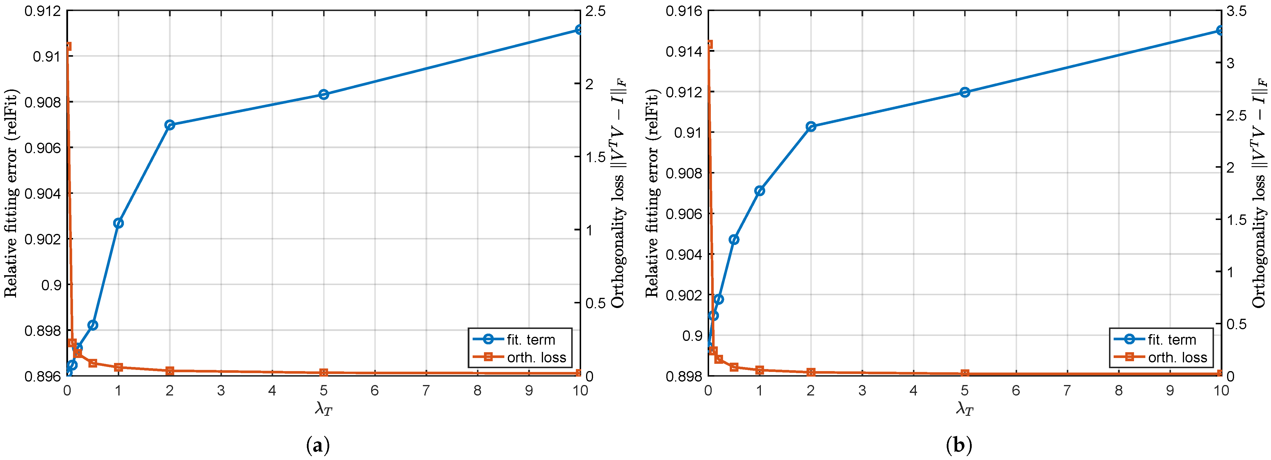
In the first stage, we fix ${\lambda }_S$ and vary ${\lambda }_V$ over a prescribed range. For each fixed ${\lambda }_S$, we plot the relative data fitting error $\parallel \mathcal{X} -〚\mathbf{W},\mathbf{S},\mathbf{V}{〛\parallel }_F^2/{\parallel \mathcal{X}\parallel }_F^2$ and the orthogonality loss $\parallel {\mathbf{V}}^T{\mathbf{V}-\mathbf{I}\parallel }_F^2$ in the same figure. The values of ${\lambda }_S$ are chosen on a logarithmic grid $\mathrm{logspace}(-4,1,10)$, resulting in ten such curves. We observed that for different values of ${\lambda }_S$, the curves of both the data fitting term and the orthogonality loss term with respect to ${\lambda }_V$ exhibit highly consistent trends: the data fitting error increases monotonically, while orthogonality loss first decreases rapidly and then becomes flat. We thus only plot two representative figures with ${\lambda }_S=0.0001$ and $0.7743$ in Figure 1.

As shown in Figure 1, the orthogonality loss decreases rapidly as ${\lambda }_V$ increases from zero, but becomes nearly flat for ${\lambda }_V\gtrsim 2$. Beyond this point, further increasing ${\lambda }_V$ yields only marginal improvement in orthogonality, while the data fitting error continues to increase. Therefore, we select ${\lambda }_V=2$, which achieves near-saturated orthogonality with a limited increase in fitting error.

After fixing ${\lambda }_V=2$, we further tune the TV regularization parameter ${\lambda }_S$. Figure 2 shows the curves of the relative data fitting error $\parallel \mathcal{X} -〚\mathbf{W},\mathbf{S},\mathbf{V}{〛\parallel }_F^2/{\parallel \mathcal{X}\parallel }_F^2$ and the TV regularization term $\mathrm{trace}\left({\mathbf{S}}^{\mathrm{T}}\mathbf{L}\mathbf{S}\right)$ (3) as ${\lambda }_S$ varies on a logarithmic scale. When ${\lambda }_S\le 0.2$, the fitting error remains almost unchanged, indicating that the TV regularization has a negligible effect on the solution. As ${\lambda }_S$ increases beyond this range, the TV regularization term starts to decrease rapidly. However, for larger values of ${\lambda }_S$ (e.g., ${\lambda }_S\ge 0.5$), the relative fitting error increases noticeably, implying an over-regularization effect that deteriorates data fidelity.

Based on this trade-off, we select ${\lambda }_S=0.2$, which corresponds to the elbow point of the curve, where a substantial reduction in the TV term is achieved, while the data fitting error is less affected.

Choice of R. The choice of rank R is guided by both modeling considerations and common practice in topic modeling. On one hand, a small rank tends to produce overly coarse topics that merge distinct narrative motifs. On the other hand, too large a rank leads to many fragmented topics that contain repeated and duplicated information.

In LDA and related models, the number of topics is typically specified a priori and chosen to balance interpretability and topic resolution, rather than being optimized based on likelihood or reconstruction error. In many empirical studies, values around 6∼12 are usually adopted for exploratory analysis, especially when identifying a small number of coherent and interpretable topics. Following this convention and considering the scale of our corpus, we set $R=10$ in our experiments.

Algorithm. Algorithm 1 is applied to solve the model (5) with random initialization. The algorithm is stopped either when $max\{\parallel {\mathbf{W}}^{(k+1)}-{\mathbf{W}}^{\left(k\right)}{\parallel }_F/\parallel {\mathbf{W}}^{\left(k\right)}{\parallel }_F,\parallel {\mathbf{S}}^{(k+1)}-{\mathbf{S}}^{\left(k\right)}{\parallel }_F/\parallel {\mathbf{S}}^{\left(k\right)}{\parallel }_F,\parallel {\mathbf{V}}^{(k+1)}-{\mathbf{V}}^{\left(k\right)}{\parallel }_F/\parallel {\mathbf{V}}^{\left(k\right)}{\parallel }_F\}<{10}^{-6}$ or when 5000 iterations are reached.

5.3. Results

5.3.1. Topic Semantics: Top Vocabulary Words

We first examine the semantic content of each topic through its most representative words. Recall that the vocabulary–topic factor matrix $\mathbf{V}\in {\mathbb{R}}^{K\times R}$ encodes the contribution of each vocabulary term to each topic. Each column ${\mathbf{v}}_r$ of $\mathbf{V}$ thus corresponds to a topic-specific distribution over the vocabulary, with larger values indicating stronger association between a word and the topic. For interpretability, we rank words within each topic according to their weights in the corresponding column, and report the top-ranked terms as indicative topic descriptors.

Table 2. Top-20 representative words for each topic generated by NTF model (5).

Topic	Top Words (Top-20)
T1	black, girl, mother, white, home, boy, life, work, live, world, remember, believe, feel, hand, arm, smile, laugh, lie, die, dead
T2	house, door, room, window, kitchen, table, road, step, follow, return, water, sleep, rest, light, tree, smell, body, foot, small, high
T3	eye, head, face, mouth, finger, leg, skin, blood, lip, tooth, voice, sound, pull, drop, fall, star, green, dog, pecola, frieda
T4	father, wife, family, man, milkman, macon, pilate, hagar, reba, ruth, money, buy, store, station, car, kill, marry, guitar, folk, colored
T5	woman, child, love, black, sula, nel, eva, hannah, helene, dewey, jude, green, mamma, miss, yellow, peace, pain, dirt, medallion, tar
T6	alice, joe, violet, dorcas, malvonne, manfred, street, city, hair, blue, coat, trace, cee, mama, yes, okay, suppose, nice, crazy, hurt
T7	sethe, beloved, baby, denver, halle, paul, suggs, garner, sixo, amy, stamp, schoolteacher, ella, sweet, ghost, janey, jones, clearing, burglar, paid
T8	son, michael, christmas, dinner, bedroom, guest, closet, jade, jadine, valerian, sydney, margaret, ondine, gideon, soldier, matter, yardman, apple, turkey, boat
T9	cosey, heed, christine, junior, romen, vida, papa, sandler, hotel, suit, lawyer, bill, grandfather, beach, stair, desk, chair, reach, thumb, menu
T10	florens, blacksmith, sorror, lina, jacob, rebekka, willard, smithy, village, land, weather, horse, enter, infant, mistress, sir, twin, floren, scully, patrician

reports the most representative words for each topic.

Notably, Topics 1 and 2 appear to be the strongest candidates for cross-work shared topics in the Morrison corpus, as will be further supported in the next subsection. Topic 1 is characterized by words such as ‘mother’, ‘black’, ‘white’, ‘remember’, and ‘die’. These lexical patterns may be read as pointing to the persistent negotiation of identity, lineage, and the haunting presence of history (‘rememory’) that transcends any single plot; in this interpretive sense, Topic 1 may be read as reflecting an ontological dimension. Topic 2 includes ‘house’, ‘kitchen’, ‘door’, and ‘window’. These words suggest the centrality of domestic space as a recurring site where historical trauma is enacted and endured. In Morrison’s work, the house is rarely just a setting; it can be read as a witness to the bodily experiences associated with Topic 1. In this sense, Topic 2 may be read as reflecting a spatial/material dimension.

The coherence of these two topics, together with their distinct lack of character-specific names, suggests that they may be interpreted as functioning more like global/shared semantic themes than local ones. This will be further supported by the work–topic heatmap in the next subsection. The emergence of these cross-work topics also suggests that the proposed model is able to recover shared components whose lexical patterns are broadly consistent with thematic concerns frequently discussed in Morrison scholarship [28,29,30], especially the articulation of racialized identity through everyday bodily experience and domestic life.

On the other hand, a subset of topics appears to be more novel-specific, characterized by the presence of character names and plot-related terms. For example, Topic 3 prominently features Pecola and Frieda, indicating its specificity to The Bluest Eye, while Topics 4 and 5 are dominated by character vocabularies from Song of Solomon and Sula, respectively. Some topics combine character-specific and more general social vocabulary, suggesting partial overlap across novels.

5.3.2. Work–Topic Associations

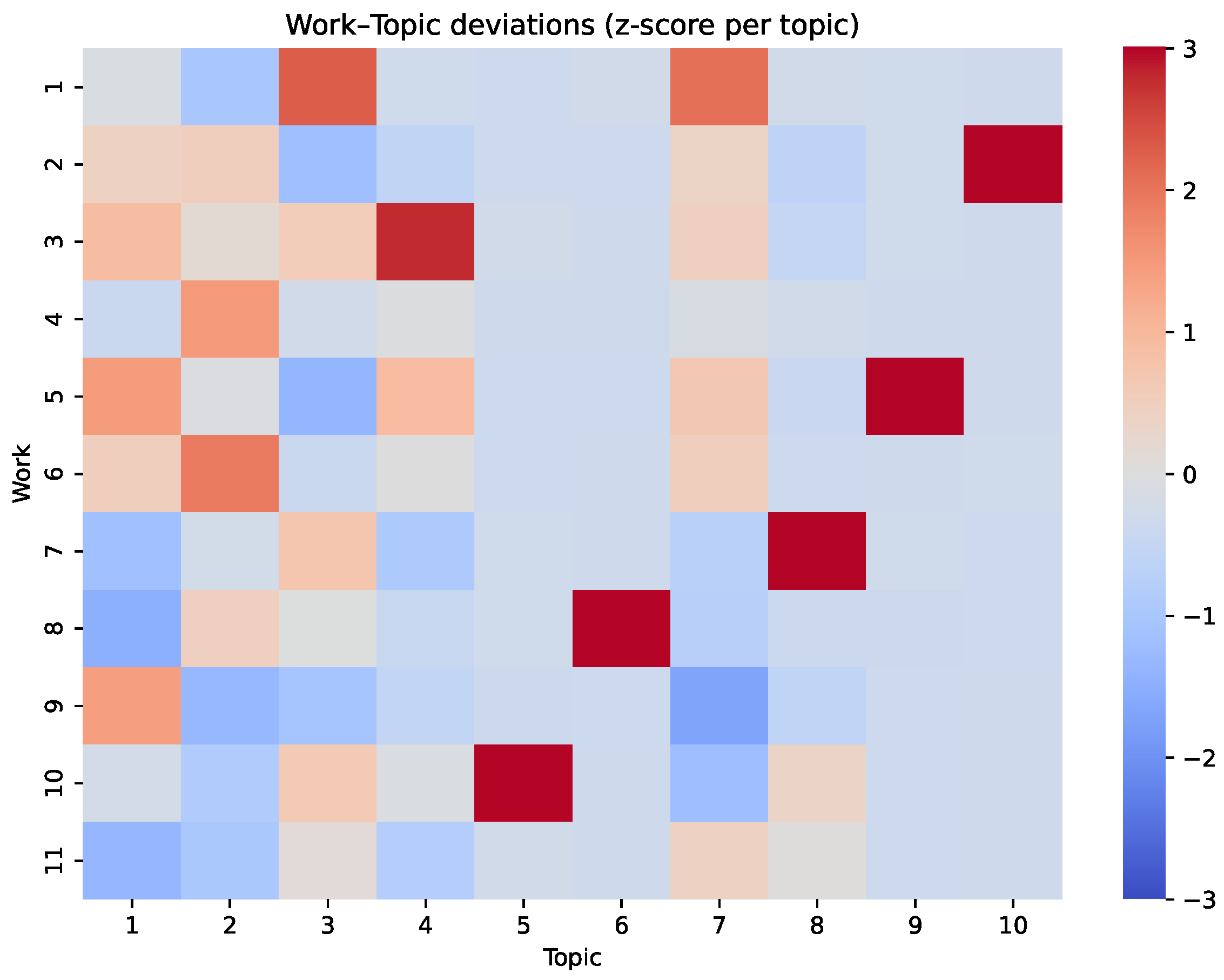
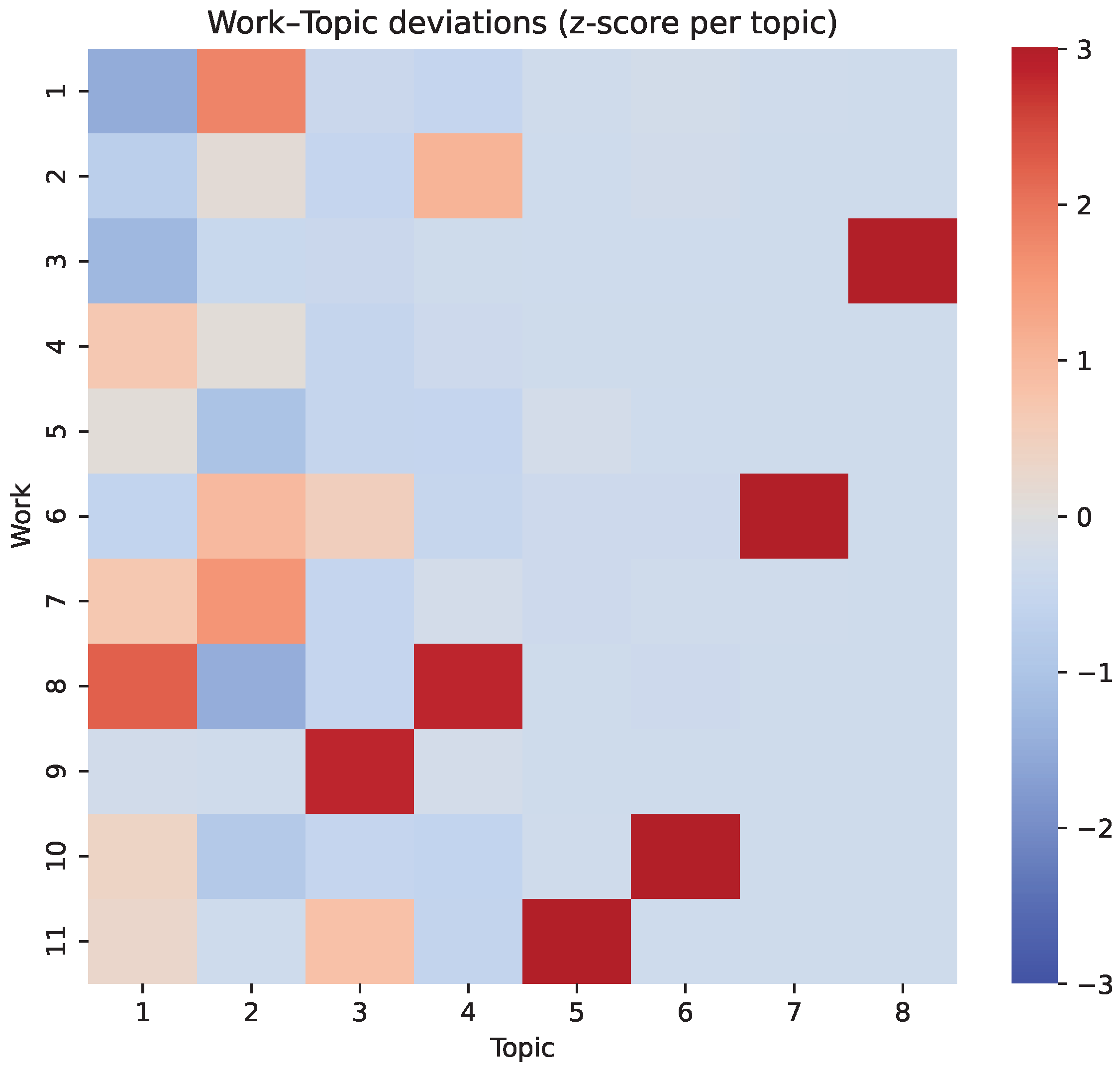
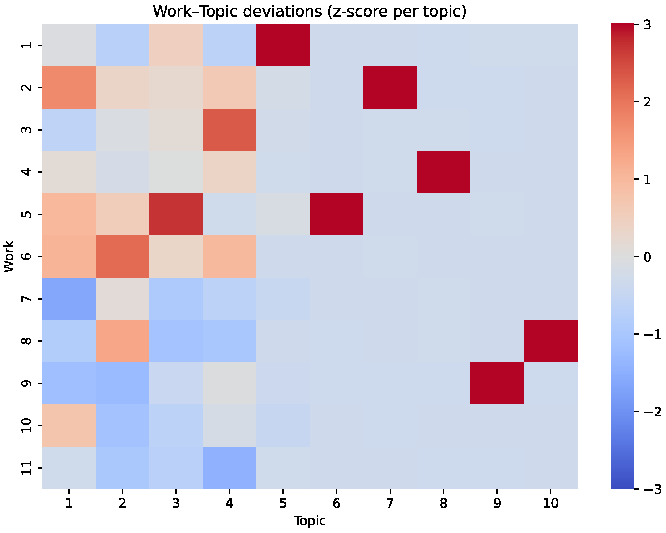
We next examine how the identified topics are associated with individual works through the work–topic factor matrix $\mathbf{W}$. Each entry of $\mathbf{W}$ represents the overall intensity of a topic within a given work. We normalize each column of $\mathbf{W}$ by applying a z-score transformation to each topic; namely, for each topic, we subtract the mean across works and divide by the corresponding standard deviation. Figure 3 visualizes the normalized factor matrix as a heatmap. Positive (red) and negative (blue) values indicate above- and below-average emphasis of a topic within a given work, respectively. This representation allows us to distinguish cross-work themes from work-specific ones.

From the figure, we observe that the first two topics (the first two columns) exhibit a more distributed intensity pattern. Unlike the later topics, Topics 1 and 2 do not concentrate exclusively on a single work. Instead, they show moderate to high activation across multiple novels. This quantitative distribution is consistent with interpreting Topics 1 and 2 as cross-work shared components rather than novel-specific ones, in line with the lexical observations in Section 5.3.1.

On the other hand, other topics display highly concentrated deviations, characterized by strong positive values in a single novel and near-average values elsewhere. For example, Topic 3 exhibits a pronounced peak associated with The Bluest Eye (Work 1), while Topics 4 and 5 are strongly aligned with Song of Solomon (Work 3) and Sula (Work 2), respectively. In contrast to the vocabulary-based inspection in Section 5.3.1, these concentrated deviations provide a quantitative perspective on the work-specific nature of these topics.

From the perspective of individual works, we also observe that some works (e.g., Works 7 and 11) exhibit z-scores close to zero across all topics. This indicates that, with respect to the extracted topics, these works do not show pronounced deviations from the corpus-level mean for any single topic.

5.3.3. Topic Profiles over Narrative Position

To analyze how topics evolve along the narrative timeline, we focus on how each topic is actually realized within individual works at different narrative positions. Recall that in the proposed model, the factor $\mathbf{S}$ encodes narrative templates that are shared across works, while the factor $\mathbf{W}$ controls the overall participation strength of each topic within a specific work. Neither factor alone captures how a topic manifests at a concrete narrative position. We therefore consider their combined contribution. For each work i, narrative segment j, and topic r, the realized topic intensity is given by the product $W_{i,r}{S}_{j,r}$. To remove scale ambiguity and enable meaningful comparison across topics and works, we define the topic responsibility

$$p_{i,j,r}={\displaystyle \frac{W_{i,r}{S}_{j,r}}{{\sum }_{r^{\prime }=1}^R{W}_{i,r^{\prime }}{S}_{j,r^{\prime }}}},$$

which measures the relative emphasis of topic r at narrative position j within work i. This representation provides a descriptive view of how topic emphasis is distributed along the narrative timeline, allowing one to distinguish between topics that have relatively stable presence and those showing more localized variation.

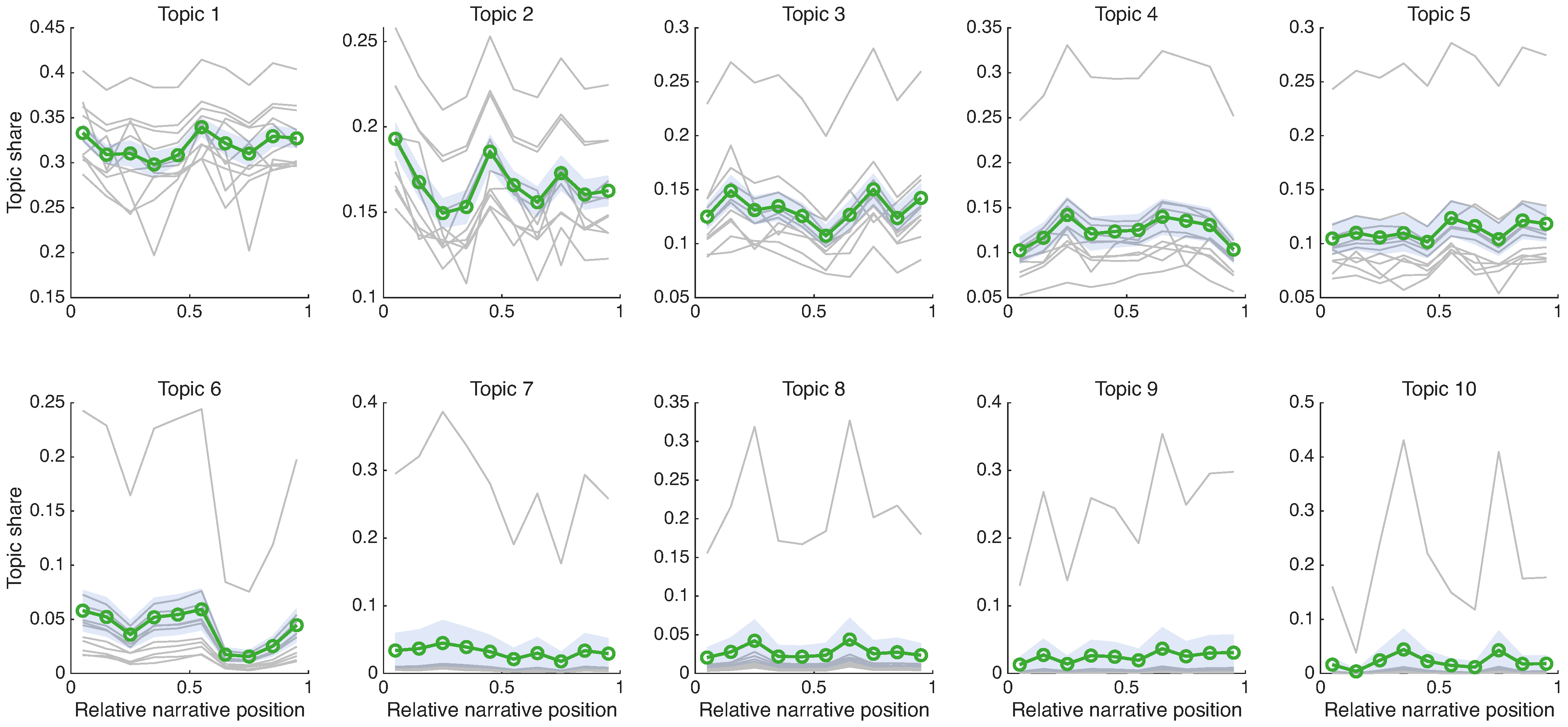
Figure 4 visualizes the topic curves $p_{i,j,r}$ over the narrative timeline for all topics. Thin gray curves represent individual works, while thick colored curves show the average trajectory across works, with shaded regions indicating standard errors. We make several descriptive observations:

Topics 1 and 2 exhibit relatively stable trajectories across the narrative timeline, with only mild fluctuations around their mean levels. Combined with their distributed presence across works, observed in Section 5.3.2, and their vocabulary profiles highlighted in Section 5.3.1, this stability is consistent with their interpretation as cross-work themes that permeate narratives rather than concentrating on specific events or plot points.

For Topics 3–10, a markedly different pattern can be observed. In these cases, we can observe that one individual work exhibits consistently higher values across narrative positions, while the remaining works stay much lower. As a result, the average trajectory remains low despite the presence of a prominent curve in a single work.

For some work-specific topics (e.g., Topics 6–10), the dominant curves exhibit noticeable fluctuations across narrative positions. This indicates that, within the associated work, the relative emphasis of the topic is not uniformly distributed along the narrative timeline. Such variations reflect localized differences in how the topic is realized within a single work, under the overall dominance of that work.

Overall, the topic curves offer a complementary, coarse-grained summary of how topic emphasis is distributed along narrative position, supporting the distinction between relatively stable cross-work themes and more localized, work-dependent components.

5.3.4. Summary

Taken together, the analyses of topic vocabularies, work–topic associations, and narrative topic curves support the distinction between cross-work shared topics and work-specific topics in Morrison’s fiction.

Topics 1 and 2 emerge as the strongest candidates for broadly shared topics across the corpus. They are characterized by words related to bodily experience, family relations, domestic spaces, and everyday social interactions, including recurrent references to black–white identity (Section 5.3.1). At the work level, they exhibit relatively uniform intensity across novels (Section 5.3.2), and at the narrative level, their topic curves show stable profiles with only mild fluctuations (Section 5.3.3). These patterns are also broadly consistent with thematic concerns frequently discussed in Morrison scholarship, suggesting that the proposed model is able to recover cross-work components that are interpretable in a literary context.

In contrast, Topics 3–10 consistently display strong concentration within individual novels. Their vocabularies are dominated by character names and plot-related terms, their work–topic associations show sharp peaks for specific works, and their narrative curves are largely driven by a single dominant trajectory. These topics may be interpreted as reflecting more localized thematic structures that are specific to individual narratives.

5.4. Comparisons with NMF Model

We consider a nonnegative matrix factorization (NMF) model constructed from the same corpus as a comparison. We first construct the matrix. Following the preprocessing steps described in Section 3.1, including tokenization, stopword removal, and vocabulary selection, we first build a global vocabulary of size K shared across all works. Unlike the tensor construction, we do not distinguish narrative segments. Instead, for each work, all word occurrences are aggregated into a single bag-of-words representation. This yields a nonnegative work–vocabulary matrix $\mathbf{X}\in {\mathbb{R}}_{+}^{I\times K}$, where each entry records the normalized frequency of a vocabulary word within a given work.

To ensure a fair comparison with the tensor-based model, we also impose the orthogonality regularization on $\mathbf{V}$. The resulting NMF model is thus formulated as

$$\begin{array}{cc}\hfill \underset{\mathbf{W},\mathbf{V}}{min}& {\displaystyle \frac{1}{2}}{\parallel \mathbf{X}-\mathbf{W}{\mathbf{V}}^T\parallel }_F^2+{\displaystyle \frac{{\lambda }_V}{2}}{R}_{orth}\left(\mathbf{V}\right)\hfill \\ \hfill \mathrm{s}.\mathrm{t}.& \mathbf{W}\in {\mathbb{R}}_{+}^{I\times R},\mathbf{V}\in {\mathbb{R}}_{+}^{K\times R},\parallel {\mathbf{v}}_r\parallel =1,r=1,\dots ,R.\hfill \end{array}$$

(28)

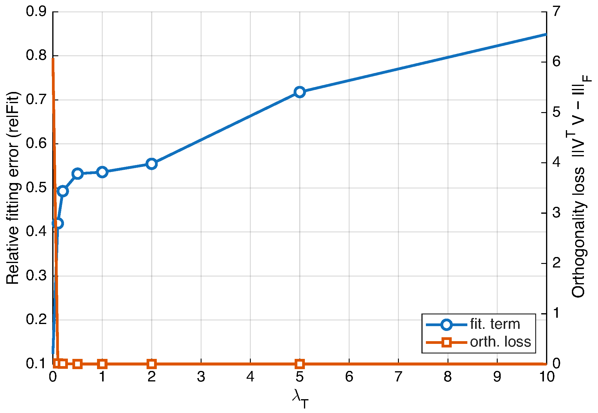
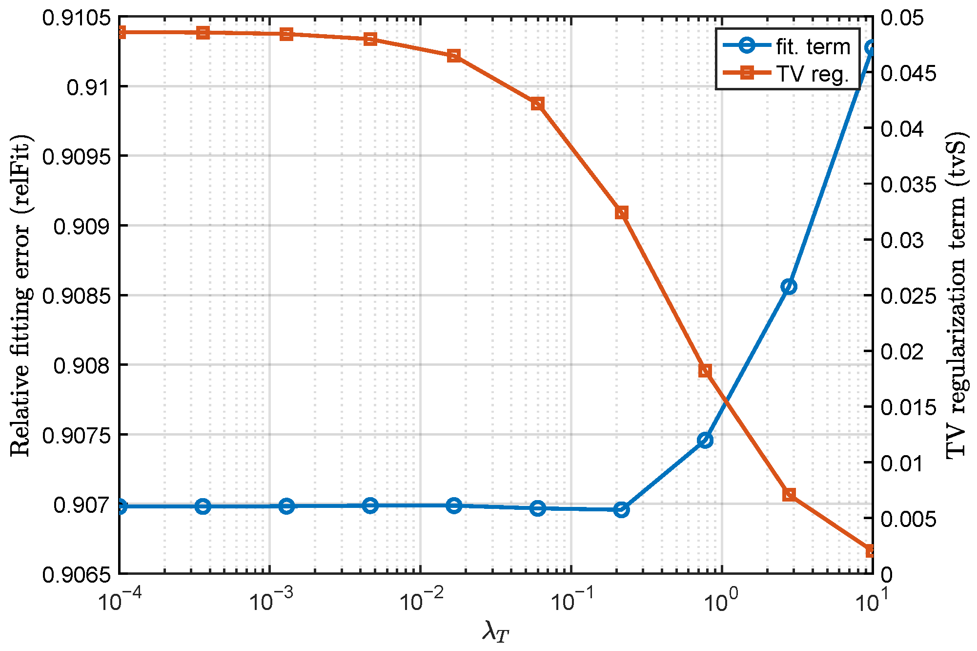
We also solve it using an algorithm similar to Algorithm 1. We tune ${\lambda }_T$ in the above model in a similar way to that described in Section 5.2. The curves are plotted in Figure 5, based on which we choose ${\lambda }_T=0.1$ in the model.

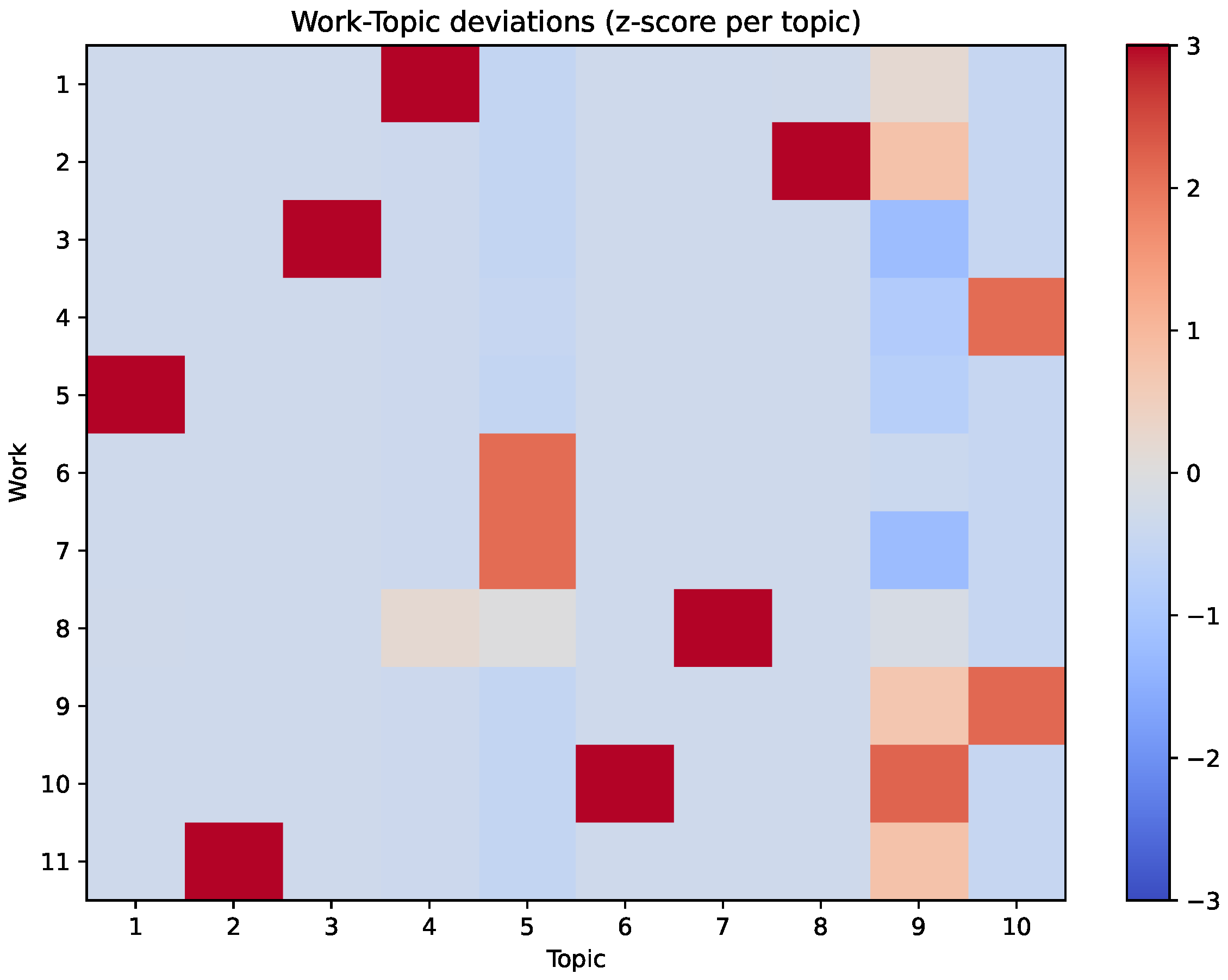
The top vocabulary words and the work–topic association heat map are respectively provided in

Table 3. Top-20 representative words for each topic generated by NMF model (28).

Topic	Top Words (Top-20)
T1	man, eye, head, child, face, mother, boy, smile, live, hair, home, water, laugh, die, arm, world, mouth, step, young, small
T2	woman, door, room, light, street, bed, son, finger, hard, touch, dress, table, violet, wonder, dark, care, grow, valerian, listen, color
T3	car, kitchen, throw, rest, mama, deep, daddy, frieda, early, dance, gold, visit, ago, business, offer, refuse, feed, fine, save, reverend
T4	hand, feel, life, work, foot, milkman, sleep, dead, remember, tree, guitar, pick, kill, pull, pilate, wife, start, macon, sweet, real
T5	cee, lenore, lily, lotus, doctor, sarah, salem, ethel, locke, georgia, billy, jackie, mike, beau, army, korea, thelma, ida, patient, prince
T6	heed, christine, cosey, junior, sandler, romen, hotel, vida, beach, papa, bill, grandfather, guest, roman, correctional, cannery, settlement, manila, menu, resort
T7	house, girl, white, love, black, lie, father, believe, new, eat, begin, money, window, fall, blue, stay, play, leg, town, kind
T8	big, miss, mavis, bad, return, hat, star, inside, school, dream, buy, consolata, lady, tear, folk, coffee, order, gigi, beautiful, misner
T9	sethe, denver, beloved, baby, paul, suggs, halle, garner, sixo, stamp, schoolteacher, amy, ella, em, jones, sweet, paid, janey, ghost, milk
T10	sula, nel, eva, hannah, dewey, shadrack, helene, jude, mamma, medallion, river, plum, peace, tar, ajax, valley, hill, wright, boyboy, newly

and Figure 6. Upon comparing the proposed model with the NMF-based model, we have the following observations:

• Both the NTF and NMF models yield a similar macroscopic structure in the work–topic association heatmaps (Figure 3 and Figure 6). In both cases, we observe that the first two topics behave as global (author-level) themes, whereas the remaining topics are predominantly work-specific. This commonality suggests that the Morrison corpus simultaneously contains (i) a small number of shared thematic structures and (ii) several work-specific cores, and that such a global-local mixture is robust to the choice of factorization model.
• Despite this shared global–local pattern, the two models differ substantially in what they place into the global themes. Inspecting the representative words (Table 2 and Table 3), we find that the global topics extracted by our NTF model are more readily interpretable as corpus-level shared thematic patterns in Morrison’s fiction. Noticeably, NTF Topic 1 aggregates words directly tied to Morrison’s recurrent themes: racial polarity and social structure (‘black’, ‘white’), kinship and home (‘mother’, ‘home’), and the ethical weight of memory and mortality (‘remember’, ‘die’, ‘dead’). These lexical cues can be read as forming a more coherent thematic pattern that is consistent with a corpus-level reading of Morrison’s oeuvre. In contrast, the corresponding global topic in NMF is dominated by broadly ubiquitous narrative vocabulary (e.g., generic human referents and body-related terms such as ‘man’, ‘child’, ‘eye’ (which may be specific to the novel The Bluest Eye), ‘head’, and ‘face’, together with common verbs and everyday descriptors). While such words naturally appear across all novels and produce a global topic under work-level co-occurrence, they are less indicative of a Morrison-specific shared thematic pattern and instead more closely resemble a corpus-agnostic narrative “background” component.
• A similar but subtler difference appears in the second global topic. Both models identify a shared topic organized around domestic and spatial lexicons (e.g., ‘house’, ‘door’, ‘room’, ‘window’, ‘kitchen’, ‘bed’), but NTF yields a more structured semantic field that links interior spaces to movement and recurrence (e.g., ‘road’, ‘step’, ‘follow’, ‘return’), and to embodied perception (e.g., ‘smell’, ‘body’). This coupling is broadly consistent with existing discussions in literary studies that treat space not merely as a setting but as a carrier of social relations and narrative progression. By comparison, NMF’s analogous topic tends to mix household objects and everyday descriptors in a less coherent directed manner, again reflecting document-level aggregation effects.

In a nutshell, NMF compresses each long novel into a single document-term vector, so its “global” topics tend to be dominated by corpus-agnostic, high-frequency narrative vocabulary. In contrast, NTF incorporates an additional mode for narrative progression, which provides extra structure for aligning recurrent patterns across works beyond overall co-occurrence (even though the heatmap visualizes the work–topic marginal). This may partly explain why the global topics extracted by NTF are more interpretable as cross-novel shared thematic patterns, e.g., race (black/white), kinship/home, memory and mortality, and domestic space, whereas NMF’s shared topics more closely resemble a generic narrative background component.

5.5. Comparison with LDA Model

We further compare our NTF model with the standard LDA model, which is widely used in digital humanities and text mining. The LDA model is also trained on the same Morrison corpus under the same preprocessing as in Section 3.1. We also build a global vocabulary shared across all works and represent each novel as a single bag-of-words document, resulting in a work–vocabulary matrix similar to that in the NMF model. We run LDA using the Gensim package in Python 3.12 (Gensim is an open-source Python library designed for unsupervised topic modeling, document indexing, and similarity retrieval) with the number of topics also set to 10 for a direct comparison. The top vocabulary words and the work–topic heatmap are respectively presented in

Table 4. Top-20 representative words for each topic generated by the LDA model.

Topic	Top Words (Top-20)
T1	paul, boston, rifle, lard, ax, solid, pies, potato, debt, rocker, hominy, i’m_telling, hears, carolina, thirsty, alley, sap, little_bit, plank, wells
T2	gigi, couple, streets, pool, remember, voice, wine, modern, strange, old_woman, tomorrows, america, folks, california, cold, simply, sure, concert, woman, heard
T3	sethe, denver, beloved, baby, paul, suggs, halle, stamp, schoolteacher, amy, ella, sweet, jones, janey, stone, black, bodwin, ghost, milk, paid
T4	sula, nel, eva, hannah, jude, dewey, helene, shadrack, plum, ajax, tar, peace, medallion, wright, boyboy, newly, river, valley, hill, nelson
T5	florens, blacksmith, jacob, rebekka, willard, sorror, lina, smithy, patrician, scully, village, land, horse, weather, mistress, twin, sir, enter, infant, floren
T6	rye, fast, lie, hard, boy, sure, train, words, eyes, talk, father, kind, road, head, house, town, open, voice, money, world
T7	cow, chickens, girls, kitchen, coffee, cake, sugar, butter, eggs, bread, flour, potatoes, garden, stove, table, dishes, milk, pan, pie, supper
T8	fool, truth, inside, dream, beautiful, bad, return, order, coffee, folk, buy, hat, miss, star, school, mavis, consolata, gigi, lady, misner
T9	mountain, trees, river, flowers, birds, sun, sky, wind, water, earth, field, grass, stone, road, light, dark, house, town, morning, night
T10	milkman, macon, pilate, hagar, reba, ruth, guitar, dead, remember, tree, kill, wife, father, family, money, buy, store, station, folk, colored

and Figure 7. We make the following observations:

• Table 4 shows that several LDA topics are dominated by character names and plot-specific entities (e.g., Sethe, Denver, Beloved, Sula, Nel, Eva, Milkman, Pilate, Macon), indicating that LDA can effectively identify work-specific lexical clusters. This is also reflected in the heatmap in Figure 7 (see, e.g., Topics 1–4, and 6–8), where several topics exhibit a pronounced positive deviation concentrated on a single work.
• In Figure 7, Topics 5, 9, and 10 appear more like “global” themes in the sense that they do not show an equally sharp peak for a single work, as is the case with some other topics. However, their top words (Table 4) do not form a coherent thematic cluster that can be easily interpreted as a Morrison-specific cross-novel thematic pattern. For example, Topic 5 is dominated by a set of character names and plot entities (e.g., ‘Florens’, ‘Blacksmith’, ‘Jacob’, ‘Rebekka’, ‘Lina’, ‘Sorrow’), which strongly suggests that it is a novel-anchored signature (here closely tied to A Mercy) rather than an author-level structure; its seemingly non-peaked pattern can be described as a diffuse or mixed assignment in the document-topic proportions. A similar phenomenon appears in Topic 10, which is driven by character names (‘Macon’, ‘Pilate’, ‘Hagar’, ‘Reba’, ‘Ruth’) together with generic social vocabulary (e.g., ‘family’, ‘money’, ‘buy’, ‘store’). By contrast, Topic 9 consists almost entirely of generic nature-and-setting vocabulary (e.g., ‘mountain’, ‘trees’, ‘river’, ‘flowers’, ‘sun’, ‘sky’, ‘wind’, ‘water’, ‘morning’, ‘night’). Such scenic terms naturally recur across many novels and are thus prone to appear as a broad “global” component in the LDA results, but they are corpus-agnostic and only weakly indicative of Morrison’s thematic concerns. In summary, these “global-looking” topics do not align with the Morrison-diagnostic global themes (e.g., racialized identity, kinship/home, memory/mortality, and domestic space).

5.6. Comparison with the Standard NTF Model

We also consider a standard nonnegative tensor factorization (NTF) model as a baseline. Specifically, we solve

$$\begin{array}{c}\hfill \underset{\mathbf{W},\mathbf{S},\mathbf{V}}{min}{\displaystyle \frac{1}{2}}\parallel \mathbf{X}-〚\mathbf{W},\mathbf{S},\mathbf{V}{〛\parallel }_F^2\mathrm{s}.\mathrm{t}.\mathbf{W},\mathbf{S},\mathbf{V}\in {\mathbb{R}}_{+}.\end{array}$$

(29)

The top vocabulary words and the work–topic association heat map are respectively provided in

Table 5. Top-20 representative words for each topic generated by the standard NTF model (29).

Topic	Top Words (Top-20)
T1	eye, child, hand, love, life, feel, home, house, live, black, work, head, white, room, mother, remember, girl, laugh, cherish, scheme
T2	woman, girl, house, hand, mother, door, work, child, white, head, feel, room, hair, smile, light, home, life, cherish, freely, skinny
T3	face, eye, head, man, boy, hand, baby, water, smile, door, girl, house, foot, black, white, hair, room, sleep, feel, light
T4	man, woman, house, milkman, white, head, black, mother, child, love, life, work, feel, father, live, hand, smile, agitate, dart, recognition
T5	eye, blue, yes, bluer, girl, head, pecola, feel, black, love, white, hand, baby, die, frieda, face, sleep, arm, house, remember
T6	sethe, denver, beloved, baby, paul, suggs, mother, sweet, wink, inhale, skinny, cherish, couch, withhold, christian, remembrance, recognition, pedestrian, liar, dart
T7	sula, nel, eva, boy, hannah, lie, door, black, love, peace, water, chicken, smile, eye, feel, jude, friend, miss, bed, child
T8	valerian, margaret, sydney, ondine, jadine, son, michael, street, kitchen, table, room, yes, christmas, sleep, eat, believe, hair, jade, pattern, couch
T9	lina, sorrow, mistress, sir, twin, florens, sleep, blacksmith, eye, floren, baby, tree, house, girl, new, fall, child, die, patrician, pattern
T10	heed, christine, junior, cosey, hotel, room, papa, smile, friend, hand, dart, recognition, remembrance, christian, withhold, couch, liar, skinny, tenant, elaborate

and Figure 8. Upon comparing this model with with the proposed NTF model, we make the following observations:

• Table 5 shows that the standard NTF model can also identify several work-specific topics. This is reflected in Figure 8, where Topics 5–10 exhibit pronounced positive deviations concentrated on individual works.
• Compared with the proposed NTF model, the main difference lies in the organization of the shared-theme topics. In Figure 8, Topics 1–4 show some cross-work distribution, but their representative words overlap substantially and form relatively broad lexical fields. For example, words such as ‘hand’, ‘house’, ‘mother’, ‘child’, ‘white’, ‘black’, ‘feel’, and ‘life’ recur across Topics 1–4. By contrast, in the proposed model, the first two topics (see Table 2 and Figure 3) are more clearly separated and are more readily interpretable as two complementary cross-work themes, as discussed in Section 5.3.1. This difference may reflect that, without additional structural constraints, the shared themes extracted by standard NTF are more likely to overlap, whereas the proposed model appears to yield a more clearly organized shared-theme layer.

5.7. Additional Validations on Works of Hemingway and Swift

To further examine the effectiveness of the proposed model beyond the Morrison corpus, we additionally apply it to the long novels of Ernest Hemingway and Graham Swift in the following two subsections.

5.7.1. Hemingway’s Novels

Ernest Hemingway’s corpus consists of ten book-length novels, spanning from The Torrents of Spring (1926) to True at First Light (1999), as summarized in

Table 6. Ernest Hemingway’s ten novels.

Work	Year	Tokens
The Torrents of Spring	1926	8312
The Sun Also Rises	1926	22,680
A Farewell to Arms	1929	27,485
To Have and Have Not	1937	17,504
For Whom the Bell Tolls	1940	57,868
Across the River and Into the Trees	1950	21,645
The Old Man and the Sea	1952	10,556
Islands in the Stream	1970	47,441
The Garden of Eden	1986	19,368
True at First Light	1999	39,183

. Hemingway (1899–1961), a Nobel Laureate in Literature, is widely recognized for portraying modern experience through emotional restraint, bodily states, and understated interpersonal relations. Across his fiction, critics have repeatedly noted a focus on fatigue, injury, intimacy, and the difficulty of articulation, with meaning often conveyed through silence, repetition, and everyday routines rather than explicit psychological explanation [34,35].

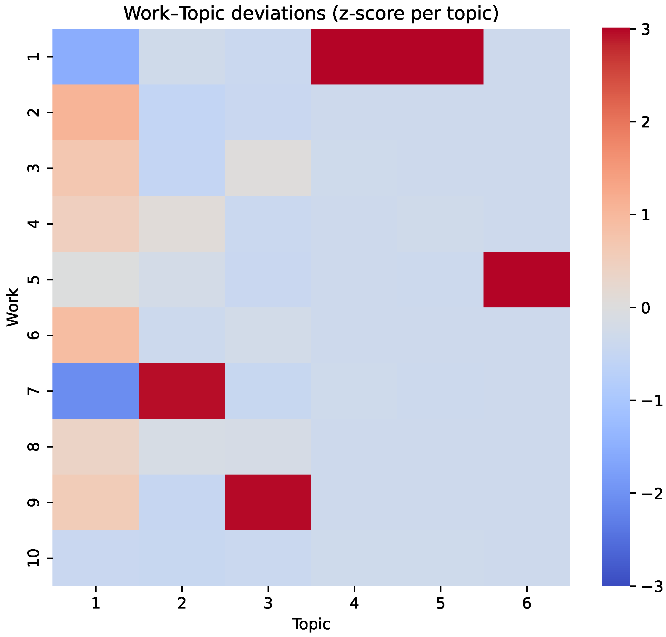
The data tensor constructed from Hemingway’s works is of size $10\times 100\times 5000$. We set $R=6$ to balance interpretability and thematic coherence. In contrast, we observed that larger R produces unmeaningful topics (e.g., when $R=8$, the model produces a topic that includes the numbers of the chapters, such as ‘vii’, ‘xviii’, ‘xiv’, ‘ix’, and so on). The top vocabulary words and the work–topic heatmap are respectively presented in

Table 7. Top-20 representative words for each topic generated by the NTF model (Hemingway corpus).

Topic	Top Words (Top-20)
T1	feel, drink, yes, colonel, big, head, love, start, work, bad, bring, light, face, sleep, dark, road, room, woman, robert, lie
T2	man, fish, line, boy, water, hand, great, boat, shark, pull, sun, skiff, fast, sea, cut, eat, left, hit, rise, hook
T3	david, catherine, girl, marita, kiss, story, lunch, swim, write, devil, mirror, father, beach, madame, monsieur, elephant, burn, read, heiress, sorry
T4	scripps, bird, waitress, mandy, diana, drummer, elderly, dear, home, wife, telegrapher, story, pump, wonder, counter, voice, mercury, james, mother, scripp
T5	yogi, indian, chief, white, indians, johnson, tall, red, war, beanery, dog, grunt, pump, reader, pool, remark, factory, spring, skunk, wampum
T6	granero, pilar, jordan, maria, snow, pablo, thee, thy, agustin, sordo, fear, primitive, va, ingles, karkov, don, joaquin, que, gaylord, ingle

and Figure 9. We make the following observations:

From Figure 9, we observe that Topic 1 exhibits a global pattern across Hemingway’s novels. Table 7 illustrates that Topic 1 is characterized by affective and everyday-state vocabulary such as ‘feel’, ‘drink’, ‘love’, ‘sleep’, ‘dark’, ‘room’, ‘road’, ‘face’, and ‘lie’. These terms describe recurrent bodily and emotional conditions and the subdued interpersonal tensions through which experience is registered. In interpretive terms, this topic is broadly consistent with a widely recognized feature of Hemingway’s fiction: a restrained affective undercurrent in which meaning is staged through fatigue, silence, and everyday routines rather than explicit exposition.

On the other hand, the heatmap shows that the remaining topics display local themes. A clear example is Topic 2. It is dominated by sea-fishing and embodied action vocabulary (e.g., ‘fish’, ‘sea’, ‘boat’, ‘line’, ‘hook’, ‘pull’, ‘hand’). As shown in the heatmap, this topic exhibits a strong positive deviation in Work 7 (The Old Man and the Sea). This pattern is broadly consistent with common literary discussions: The Old Man and the Sea focuses almost entirely on sea fishing and physical endurance, whereas similar motifs play a much less prominent role in Hemingway’s other novels. The model therefore identifies this topic as more novel-specific than corpus-wide.

5.7.2. Graham Swift’s Novels

Graham Swift’s corpus consists of eleven book-length novels, summarized in

Table 8. Graham Swift’s eleven novels.

Work	Year	Tokens
The Sweet-Shop Owner	1980	24,560
Shuttlecock	1981	22,861
Waterland	1983	45,038
Out of This World	1988	18,525
Ever After	1992	29,379
Last Orders	1996	23,085
The Light of Day	2003	20,886
Tomorrow	2007	20,909
Wish You Were Here	2011	30,322
Mothering Sunday	2016	9720
Here We Are	2020	12,511

. Swift (b. 1949) is widely recognized for narratives that look backward: his fiction repeatedly returns to memory, family bonds, and the way private lives are shaped by larger histories. Rather than relying on grand plot turns, Swift often builds meaning through recollection, everyday detail, and the uneasy gap between what is told and what is withheld [36,37].

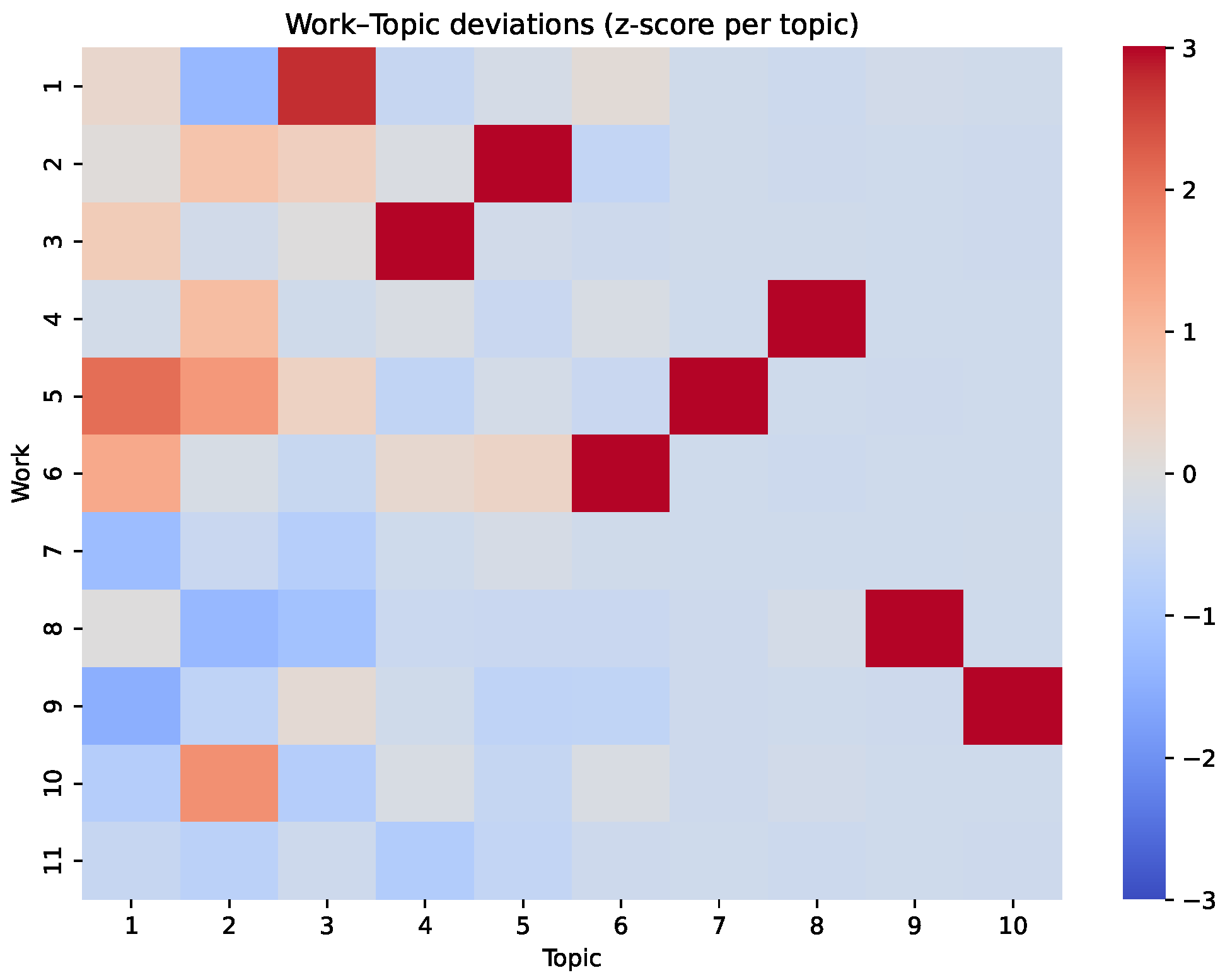
The data tensor constructed from Swift’s works is of size $11\times 100\times 5000$. We set $R=8$. The top vocabulary words and the work–topic heatmap are respectively presented in

Table 9. Top-20 representative words for each topic generated by the NTF model (Swift corpus).

Topic	Top Words (Top-20)
T1	life, father, world, war, house, remember, new, home, real, story, live, woman, far, love, ago, mother, picture, matter, lie, boy
T2	man, face, eye, head, door, car, window, end, smile, shop, girl, point, pass, street, air, road, arm, inside, step, white
T3	jack, tom, ellie, luxton, major, richards, jebb, luke, michael, brother, big, gun, farm, letter, army, soldier, vera, cow, marleston, coffin
T4	dad, grandpa, pete, mike, otis, uncle, helen, quinn, cat, grannie, eddie, christmas, marian, tomorrow, nick, kate, martin, tim, champagne, prisoner
T5	ronnie, lawrence, evie, mother, magic, eric, pablo, magician, stage, deane, penny, evergreen, parrot, mrs, eve, ring, agnes, brighton, audience, green
T6	ethel, niven, book, jane, maid, paul, drive, upleigh, hobday, beechwood, sheringham, milly, read, mister, bicycle, cook, library, mrs, emma, return
T7	lenny, vince, vie, jar, reckon, amy, ray, box, raysy, vincey, vic, dodds, quick, mandy, margate, coach, pier, cap, butcher, bernie
T8	johannes, atkinson, crick, eel, freddie, gildsey, leem, river, parr, thomas, mary, kessling, ale, brewery, ouse, fens, drainage, brewer, barley, henry

and Figure 10. We make the following observations:

Via Figure 10, we observe that Topics 1 and 2 seem to exhibit a global pattern. Table 9 illustrates that Topic 1 is characterized by words such as ‘life’, ‘remember’, ‘story’, ‘war’, ‘love’, ‘father’, ‘mother’, ‘home/house’, and ‘lie’. These terms point to recurring themes of family life, retrospective narration, and the pressure of history, where “truth” is frequently negotiated through storytelling and imperfect remembrance. In interpretive terms, this topic is broadly consistent with common literary discussions of Swift as a novelist of memory and inheritance, with personal relationships set against wider historical and moral contexts.

Topic 2 is dominated by concrete scene and perception vocabulary, including ‘face’, ‘eye’, ‘door’, ‘window’, ‘street’, ‘road’, ‘car’, ‘inside’, and ‘step’. These words suggest a shared narrative surface across the corpus: Swift repeatedly anchors reflection in ordinary spaces and small observed actions—moving through rooms, looking out of windows, traveling along roads—so that everyday settings become the stage where memory and tension accumulate. In this sense, Topic 2 complements Topic 1 by reflecting a relatively consistent way of writing, not just a recurring subject matter.

On the other hand, the heatmap shows that the remaining topics appear to be more local themes. In Table 9, Topics 3–8 are filled with proper names and tightly clustered story-specific terms, and in the heatmap, each of these topics shows a strong positive deviation in only one (or very few) works.

6. Conclusions

This paper targets a basic task in literary studies: identifying the major themes and recurring motifs that run through an author’s long novels via topic modeling. Instead of directly modeling an author’s corpus as a work × vocabulary matrix, we model it as a work × segment × vocabulary tensor and propose a modified nonnegative NTF model that encourages distinct topics (via orthogonality regularization) and smooth narrative progression (via ${\ell }_2$-TV regularization). We develop a block proximal linearization algorithm to solve the model and show that any limit point satisfies the KKT condition.

In our experiments, we use Toni Morrison’s eleven long novels as the main case study. The extracted cross-work themes exhibit qualitative patterns that are broadly consistent with thematic concerns frequently discussed in Morrison scholarship, and relative to NMF and LDA, they are more readily interpretable as cross-work thematic patterns in the present corpus. We further test the model on the long novels of Ernest Hemingway and Graham Swift as additional validations. In both cases, the model also yields shared topics whose lexical and distributional patterns are broadly consistent with critical discussions of the authors’ recurring thematic concerns.

More broadly, the proposed framework is intended as a distant-reading tool for long-novel corpora. Its scholarly relevance lies in offering a way to screen recurring themes across an author’s works and to distinguish them from more local, work-specific topics. At the same time, the model does not replace close reading or final literary judgment; rather, it may serve as a practical tool for identifying cross-work shared themes and work-specific topics for further literary examination.

References

1. Abrams, M.H.; Harpham, G.G. A Glossary of Literary Terms, 9th ed.; Wadsworth Cengage Learning; Cengage: Stamford, CT, USA, 2009. [Google Scholar]
2. Frye, N. Anatomy of Criticism: Four Essays; Princeton University Press: Princeton, NJ, USA, 2020. [Google Scholar]
3. Moretti, F. Conjectures on World Literature. New Left Rev. 2000, 2, 54–68. [Google Scholar] [CrossRef]
4. Moretti, F. Distant Reading; Verso: London, UK, 2013. [Google Scholar]
5. Jockers, M.L. Macroanalysis: Digital Methods and Literary History; University of Illinois Press: Urbana, IL, USA, 2013. [Google Scholar]
6. Li, D.; Wu, K.; Lei, V. Applying Topic Modeling to Literary Analysis: A Review. Digit. Stud. Lang. Lit. 2024, 1, 113–141. [Google Scholar] [CrossRef]
7. Meeks, E.; Weingart, S. The Digital Humanities Contribution to Topic Modeling. J. Digit. Humanit. 2012, 2, 1–6. [Google Scholar]
8. Callaway, E.; Turner, A.; Stone, E.; Halstrom, A. The Push and Pull of Digital Humanities: Topic Modeling. Digit. Humanit. Q. 2020, 14, 1–14. [Google Scholar] [CrossRef]
9. Blei, D.M.; Ng, A.Y.; Jordan, M.I. Latent Dirichlet Allocation. J. Mach. Learn. Res. 2003, 3, 993–1022. [Google Scholar]
10. Buurma, R.S. The Fictionality of Topic Modeling: Machine Reading Anthony Trollope’s Barsetshire Series. Big Data Soc. 2015, 2, 2053951715610591. [Google Scholar] [CrossRef]
11. Navarro-Colorado, B. On Poetic Topic Modeling: Extracting Themes and Motifs from a Corpus of Spanish Poetry. Front. Digit. Humanit. 2018, 5, 15. [Google Scholar] [CrossRef]
12. Ciotti, F. Distant Reading in Literary Studies: A Methodology in Quest of Theory. Testo Senso 2021, 23, 195–213. [Google Scholar]
13. Schröter, J.; Du, K. Validating Topic Modeling as a Method of Analyzing Sujet and Theme. J. Comput. Lit. Stud. 2022, 1, 1–20. [Google Scholar] [CrossRef]
14. Lee, D.D.; Seung, H.S. Learning the Parts of Objects by Non-negative Matrix Factorization. Nature 1999, 401, 788–791. [Google Scholar] [CrossRef] [PubMed]
15. Sherstinova, T.; Martynenko, G.; Zakharova, O.; Anisimova, T.; Skrebtsova, T.; Bolotova, I.; Zamiraylova, A. Topic Modelling with NMF versus Expert Topic Annotation: A Case Study on Russian Fiction. In Advances in Soft Computing; Lecture Notes in Computer Science; Springer: Berlin/Heidelberg, Germany, 2020. [Google Scholar] [CrossRef]
16. Mihajlov, T.; Petrović, V.; Marjanović, I.; Todorović, B.; Cvetanović, V. Topic Modeling of the SrpELTeC Corpus: A Comparison of NMF, LDA, and BERTopic. In Proceedings of the 2024 Federated Conference on Computer Science and Information Systems (FedCSIS), Belgrade, Serbia, 8–11 September 2024. [Google Scholar] [CrossRef]
17. Greene, D.; O’Sullivan, J.; O’Reilly, D. Topic Modelling Literary Interviews from The Paris Review. Digit. Scholarsh. Humanit. 2024, 39, 142–153. [Google Scholar] [CrossRef]
18. Hearst, M.A. TextTiling: Segmenting Text into Multi-paragraph Subtopic Passages. Comput. Linguist. 1997, 23, 33–64. [Google Scholar]
19. Riedl, M.; Biemann, C. TopicTiling: A Text Segmentation Algorithm Based on LDA. In Proceedings of the ACL 2012 Student Research Workshop; Association for Computational Linguistics: Stroudsburg, PA, USA, 2012; pp. 37–42. [Google Scholar]
20. Li, W.; Matsukawa, T.; Saigo, H.; Suzuki, E. Context-aware latent dirichlet allocation for topic segmentation. In Proceedings of the Pacific-Asia Conference on Knowledge Discovery and Data Mining; Springer: Berlin/Heidelberg, Germany, 2020; pp. 475–486. [Google Scholar]
21. Ahn, M.; Eikmeier, N.; Haddock, J.; Kassab, L.; Kryshchenko, A.; Leonard, K.; Needell, D.; Madushani, R.; Sizikova, E.; Wang, C. On large-scale dynamic topic modeling with nonnegative CP tensor decomposition. In Advances in Data Science; Springer: Berlin/Heidelberg, Germany, 2021; pp. 181–210. [Google Scholar]
22. Correia, B.; Nunes, S.; Alves, A. Dynamic Topic Modeling with Tensor Decomposition as a Tool to Explore the Legal Precedent Relevance Over Time. In Proceedings of the 23rd ACM Symposium on Document Engineering (DocEng ’23); Association for Computing Machinery: New York, NY, USA, 2023; pp. 38:1–38:12. [Google Scholar] [CrossRef]
23. Liu, Y.; Donnat, C. Tensor Topic Modeling Via HOSVD. arXiv 2024, arXiv:2501.00535. [Google Scholar] [CrossRef]
24. Cichocki, A.; Zdunek, R.; Phan, A.H.; Amari, S.i. Nonnegative Matrix and Tensor Factorizations: Applications to Exploratory Multi-Way Data Analysis and Blind Source Separation; Wiley: Chichester, UK, 2009. [Google Scholar]
25. Kolda, T.G.; Bader, B.W. Tensor Decompositions and Applications. SIAM Rev. 2009, 51, 455–500. [Google Scholar] [CrossRef]
26. Attouch, H.; Bolte, J.; Svaiter, B.F. Convergence of Descent Methods for Semi-Algebraic and Tame Problems: Proximal Algorithms, Forward-Backward Splitting, and Regularized Gauss-Seidel Methods. Math. Program. 2013, 137, 91–129. [Google Scholar]
27. Rockafellar, R.T.; Wets, R.J.B. Variational Analysis. In Grundlehren der Mathematischen Wissenschaften; Springer: Berlin/Heidelberg, Germany, 2009; Volume 317. [Google Scholar]
28. Tally, J. (Ed.) The Cambridge Companion to Toni Morrison; Cambridge University Press: Cambridge, UK, 2007. [Google Scholar]
29. O’Reilly, A. Toni Morrison and Motherhood: A Politics of the Heart; State University of New York Press: New York, NY, USA, 2004. [Google Scholar]
30. Schreiber, E.J. Race, Trauma, and Home in the Novels of Toni Morrison; Louisiana State University Press: Baton Rouge, LA, USA, 2010. [Google Scholar]
31. Morrison, T. The Site of Memory. In Inventing the Truth: The Art and Craft of Memoir; Zinsser, W., Ed.; Houghton Mifflin: Boston, MA, USA, 1987; pp. 103–124. [Google Scholar]
32. Visser, I. Relationality as Postcolonial (Self-)Referentiality in Home. Postcolonial Text 2014, 9, 1–21. Available online: https://www.google.com/url?sa=t&source=web&rct=j&opi=89978449&url=https://www.postcolonial.org/index.php/pct/article/download/1712/1684&ved=2ahUKEwiSlISAmLqTAxUlr1YBHRtIBfkQFnoECBsQAQ&usg=AOvVaw18avX1Noaqw3d40VcrORdK (accessed on 12 February 2026).
33. Nishikawa, K. Morrison’s Things: Between History and Memory; Stanford Humanities Center (Arcade): Stanford, CA, USA, 2023. [Google Scholar]
34. Donaldson, S. (Ed.) The Cambridge Companion to Hemingway; Cambridge University Press: Cambridge, UK, 1996. [Google Scholar]
35. Wyatt, D. Hemingway, Style, and the Art of Emotion; Cambridge University Press: Cambridge, UK, 2015. [Google Scholar]
36. Malcolm, D. Understanding Graham Swift; University of South Carolina Press: Columbia, SC, USA, 2003. [Google Scholar]
37. Kucała, B. Unspoken Dialogues and Non-listening Listeners in Graham Swift’s Fiction. Brno Stud. Engl. 2015, 41, 117–129. [Google Scholar] [CrossRef]
Figure 1. Tuning λ V with fixed λ S = 0.0001 (a) and λ S = 0.7743 (b). The X-axis represents λ V . The Y-axis represents the values of data fitting terms (blue curve with circle markers) and loss-of-orthogonality terms (red curve with square markers), respectively. Here we only illustrate two examples of λ S , and we observed that the trends of the curves are very similar for different values of λ S .
Mathematics 14 01106 g001
Figure 2. Tuning λ S with fixed λ V = 2 . The X-axis represents λ S . The Y-axis represents the values of data fitting terms (blue curve with circle markers) and TV regularization terms (red curve with square markers), respectively.
Mathematics 14 01106 g002
Figure 3. Work–topic association heatmap based on column-wise z-score normalization. Red and blue values indicate above- and below-average topic emphasis within a given novel, respectively. The Y-axis represents the number of works, and the X-axis represents the number of topics.
Mathematics 14 01106 g003
Figure 4. Topic curves p i , j , r over the narrative timeline. Thin gray curves correspond to individual works, while the thick colored curves show the average trajectory across works. Shaded regions indicate standard errors.
Mathematics 14 01106 g004
Figure 5. Tuning λ T . The X-axis represents λ S . The Y-axis represents the values of data fitting terms (blue curve with circle markers) and loss-of-orthogonality terms (red curve with square markers), respectively.
Mathematics 14 01106 g005
Figure 6. Work–topic association heatmap of the NMF model (28). Note that the order of works may be different from that in Figure 3 because the order of columns in W and V can be simultaneously changed.
Mathematics 14 01106 g006
Figure 7. Work–topic association heatmap of the LDA model.
Mathematics 14 01106 g007
Figure 8. Work–topic association heatmap of the standard NTF model (29).
Mathematics 14 01106 g008
Figure 9. Work–topic association heatmap of the NTF model of Hemingway’s novels.
Mathematics 14 01106 g009
Figure 10. Work–topic association heatmap of the NTF model of Graham Swift’s novels.
Mathematics 14 01106 g010