Physics-Informed Neural Network for Parameter Inference in a Tumor Model

Abstract

Mechanistic tumor growth models are widely used to describe disease progression and treatment response, but their utility depends on accurate estimation of parameters governing the underlying biological processes. In this study, we employ a Physics-Informed Neural Network (PINN) to estimate the parameters of a tumor growth model that captures both tumor dynamics and drug effects. We introduce a piecewise PINN that splits the time domain at dosing events to handle non-smooth dose-driven dynamics, and we incorporate drug injection by representing the pharmacokinetic subsystem analytically via an impulse-response function. The approach is evaluated on synthetic tumor-volume trajectories generated from known parameter sets and dosing schedules from an experimental cohort of 54 mice. Across the cohort, the PINN accurately reconstructs total tumor volume and robustly estimates the tumor proliferation rate a, with inferred values closely aligned with the true values ($R^2=0.841$). The framework was also able to estimate the drug killing effect parameter b. This consistency is further supported by forward ODE simulations using the PINN-estimated parameters. Within the evaluated setting, performance depended on the model structure, parameter identifiability, and training configuration, underscoring the need for careful loss weighting and further validation. Overall, the results demonstrate the feasibility of piecewise PINNs for parameter inference in tumor growth models and support their further study in realistic therapeutic settings.

1. Introduction

Cancer remains one of the leading causes of morbidity and mortality worldwide, with incidence rates continuing to rise, as populations age and lifestyles change [1]. Despite major advances in detection and treatment, cancer is projected to remain a dominant global health burden over the coming decades, requiring improved therapeutic strategies [2].

Mathematical modeling has become an essential tool in oncology, providing a quantitative framework to investigate tumor growth dynamics and treatment response [3,4,5]. Classical models such as the exponential, logistic, and Gompertz equations remain widely used to describe general growth patterns. Mechanistic formulations based on ordinary and partial differential equations incorporate biological processes including angiogenesis, immune–tumor interactions, and drug pharmacodynamics [6,7,8]. These models not only enable in silico exploration of therapeutic strategies that are expensive or infeasible in clinical or preclinical settings but also translate biological assumptions into a quantitative framework that supports systematic mathematical analysis and parameter inference from data.

Mathematical models have provided a framework for systematic investigation of dosing strategies beyond the conventional maximum tolerated dose (MTD) paradigm [9,10,11]. By applying these models, it becomes possible to quantify tumor dynamics and to compare expected outcomes under alternative treatment schedules. Such approaches have been proposed to reduce systemic toxicity while modulating tumor control through sustained antiangiogenic and immunomodulatory effects. By altering the tumor microenvironment, these effects may contribute to delaying or attenuating the emergence of resistant subpopulations [12,13,14,15]. In parallel, adaptive therapy has emerged as another non-conventional strategy, where drug dosing is dynamically adjusted in response to tumor burden rather than applied continuously at the maximum tolerated level [16]. Recent clinical and modeling studies suggest that such adaptive approaches, often involving treatment breaks, can suppress resistant cell populations and in some cases achieve superior outcomes compared to continuous MTD-based regimens [5]. Together, these insights emphasize that the timing, sequence, and intensity of drug administration are critical determinants of treatment efficacy and resistance dynamics.

The design of chemotherapy dosing schedules can be posed as a constrained optimization problem, where decision variables encode dose timing and magnitude, and objectives balance tumor control against treatment burden and toxicity-related limits. Optimal control formulations have been widely used to compute schedules that minimize the tumor burden (or maximize the therapeutic effect) subject to clinically motivated constraints [17,18]. Metaheuristic approaches, including genetic algorithms, provide derivative-free alternatives for searching over complex protocol spaces [19]. From an evolutionary and ecological perspective, treatment strategies have also been designed to maintain sensitive cell populations as a means of suppressing resistant clones [20,21,22]. When decisions must be made under uncertainty and partial observability, decision-theoretic formulations (e.g., Markov decision processes) provide a framework for sequential treatment planning, while Bayesian inference and machine-learning methods offer data-driven tools for adapting therapy to individual response trajectories [23,24].

The objective of the research associated with this study is to identify optimal chemotherapy schedules, defined by both dosage and timing, through the use of mathematical models [9]. Tumor–drug dynamics are represented with mechanistic tumor growth models calibrated to preclinical mouse data, where tumor dimensions are measured using digital calipers and converted to tumor volumes via geometric approximations [25]. These tumor volume measurements are then applied to estimate the parameters of the tumor models. These individualized models are subsequently used to generate personalized dosing regimens, enabling the assessment of predictive performance and systematic comparison of alternative dose-scheduling optimization algorithms.

A central component of this workflow is parameter inference from longitudinal tumor volume measurements. In practice, this inverse problem is often challenging due to measurement noise, sparse sampling, latent biological structure, and inter-animal variability. It can result in parameter estimates that fit the observed trajectories yet remain uncertain or non-unique. These limitations motivate careful diagnostics and uncertainty-aware evaluation. They also motivate focusing on new algorithms and evaluating these methods in a controlled environment, e.g., where parameters are known.

Recent studies emphasize that robust parameter inference requires explicit uncertainty quantification and careful measurement error modeling, as estimates can change substantially with the assumed likelihood, noise structure, censoring mechanisms, and model class [26,27,28,29]. Population-based approaches, including nonlinear mixed-effects (NLME) modeling, further show that parameters that are weakly informed at the individual level may become estimable when cohort-level information is incorporated [30,31]. Complementary tools, such as Fisher information analysis and optimal experimental design, have also been proposed to improve practical identifiability and to guide data acquisition [32].

Building on these identifiability considerations, we previously analyzed a reduced version of the tumor model with three state variables. Sensitivity and identifiability analyses showed that the growth rate parameter a was the most reliably identifiable from the available data, whereas the other parameters were identifiable only when initialization was sufficiently close to their true values [33]. In order to further address inter-individual variability, we applied nonlinear mixed-effects (NLME) modeling, which estimates parameters as population-level fixed effects while incorporating random effects to capture between-subject heterogeneity [31].

In this study, we evaluate Physics-Informed Neural Networks (PINNs) as a new parameter-estimation approach for a mechanistic tumor model [34]. PINNs integrate differential-equation structure into neural-network training, enabling simultaneous learning from data while enforcing the governing dynamics [35]. In inverse settings, this formulation supports the estimation of unknown parameters, coefficients, external forcings, and even reconstruction of latent (unobserved) state trajectories from sparse and noisy measurements by penalizing ODE/PDE residuals alongside data misfit [36]. In systems biology and epidemiology, ODE-constrained learning has been used to estimate unknown model parameters and to reconstruct unobserved state trajectories. For example, in compartmental epidemic models, the time-varying transmission rates have been estimated from sparse and noisy outbreak measurements [37]. In oncology, recent physics-informed studies have focused on patient- or subject-specific inference by combining mechanistic tumor models with heterogeneous clinical measurements. For example, PINNs have been used to estimate parameters in reaction–diffusion models of glioblastoma infiltration from multimodal MRI data [38]. Related digital-twin approaches reconstruct prostate cancer growth trajectories by integrating physiological modeling with longitudinal blood measurements of prostate-specific antigen and have also been used to compare alternative tumor growth laws against experimental tumor growth data [39].

In our approach, we applied an extended version of a traditional PINN architecture. In a conventional PINN architecture the loss function combines a data-misfit term with a physics-based residual that softly enforces the governing differential equations. Derivatives required for the residual are computed via automatic differentiation, enabling equation-constrained learning without repeatedly solving the ODE inside an outer optimization loop. This formulation provides a flexible way to incorporate mechanistic structure even when observations are sparse, noisy, or available only for a subset of the model states. Building on our earlier work [40], we apply PINNs to parameter estimation in a reduced two-state tumor model under a more realistic observation setting. Previously, we assumed that all state variables were directly observed; here, we align the setup with the original mice experiment, where only the total tumor volume is measured (i.e., a sum of the living and the dead tumor volumes). We focus on estimating the most reliably informed parameters (tumor growth rate (a) and maximal effect of drug (b)) and evaluate the performance in a controlled study using synthetic tumor volume trajectories generated from mouse-specific dosing schedules and parameterizations for 54 mice from experiments [9,11].

Section 2 describes the experimental measurement setting and the deterministic tumor model. It introduces the PINN formulation used for parameter inference, including the synthetic-data generation procedure used for evaluation. Section 3 presents the reconstruction and parameter-estimation results across the 54-mouse in silico cohort and includes representative convergence and consistency analyses. Finally, in Section 4, we summarize the main findings and discuss the practical advantages and limitations of the proposed method for the applied tumor model.

2. Materials and Methods

2.1. Measurement Data from Mouse Experiments

Accurate parameter estimation is essential for the design of optimized chemotherapy schedules. We employ PINNs to estimate the model parameters by fitting a mechanistic tumor growth model to in silico measurements based on parameters and doses from in vivo experimental measurements. In the animal experiments, the mice were treated with a chemotherapeutic drug called pegylated liposomal doxorubicin (PLD) [41]. During the experiments, tumor growth was monitored under the treatment by recording two orthogonal dimensions (length and width) of the subcutaneous tumors using digital calipers. The total tumor volume was then approximated under the assumption of an ellipsoidal geometry according to [25]:

$$y_{\mathrm{meas}}={\displaystyle \frac{\pi }{2}}·{(\mathrm{width}·\mathrm{length})}^{3/2}.$$

(1)

In the model, we denote by y the total tumor volume [mm³], which will be fit to $y_{\mathrm{meas}}$ data. The tumor growth was monitored until the total tumor volume reached 2000 mm³, after which the experiments were terminated in accordance with animal welfare regulations. Caliper measurements were generally performed three times per week, except on holidays or other interruptions, while chemotherapeutic injections were typically administered twice per week. These caliper-derived total tumor volumes were used as observational data during parameter estimation to fit the mathematical model [9]. The estimated parameters are then used to simulate realistic state variables.

2.2. The Applied Mathematical Model

The tumor–drug dynamics were described by a system of ordinary differential equations (ODEs) involving four state variables [34]. The state variable $x_1\left(t\right)$ represents the volume of living (proliferating) tumor cells, while $x_2\left(t\right)$ denotes the volume of dead tumor cells at time instant t, measured in ${\mathrm{mm}}^3$. The variable $x_3\left(t\right)$ models the drug concentration in blood, and $x_4\left(t\right)$ represents the drug concentration in the tissue at time t, measured in $\mathrm{mg}·{\mathrm{kg}}^{-1}$. The system dynamics is governed by the equations

$$\begin{array}{cc}\hfill {\dot{x}}_1& =(a-n)x_1-b{\displaystyle \frac{x_1{x}_3}{E{D}_{50}+x_3}},\hfill \end{array}$$

(2)

$$\begin{array}{cc}\hfill {\dot{x}}_2& =n{x}_1+b{\displaystyle \frac{x_1{x}_3}{E{D}_{50}+x_3}}-w{x}_2,\hfill \end{array}$$

(3)

$$\begin{array}{cc}\hfill {\dot{x}}_3& =-(c+k_1)x_3+k_2{x}_4+u,\hfill \end{array}$$

(4)

$$\begin{array}{cc}\hfill {\dot{x}}_4& =k_1{x}_3-k_2{x}_4,\hfill \end{array}$$

(5)

where the parameters have the interpretations listed in

Table 1. Model parameters and their biological interpretation. Units are given in $1·{\mathrm{day}}^{-1}$, except for $E{D}_{50}$, which is expressed in $\mathrm{mg}·{\mathrm{kg}}^{-1}$.

Parameter	Description
a	Tumor growth (proliferation) rate coefficient
n	Natural death rate coefficient of tumor cells, independent of therapy
b	Maximal killing effect of drug
$E{D}_{50}$	Median effective dose, controls saturation of effect
w	Clearance rate coefficient of dead tumor cells
c	Natural clearance rate coefficient of the drug from the tumor tissue
$k_1,k_2$	Inter-compartmental transfer rate coefficients between the blood ($x_3$) and the tissue ($x_4$)

.

Equation (2) describes the dynamics of living tumor cells, where the term $a{x}_1$ represents proliferation, $-n{x}_1$ accounts for natural cell death, and the saturating term $-\frac{b{x}_1{x}_3}{E{D}_{50}+x_3}$ captures drug-induced cytotoxicity as a function of drug exposure. Equation (3) governs the dead tumor cell compartment: the inflow terms $n{x}_1$ and $\frac{b{x}_1{x}_3}{E{D}_{50}+x_3}$ arise from natural death and therapy-induced killing of living cells, respectively, while $-w{x}_2$ models clearance (washout) of dead cells.

Equation (4) represents the pharmacokinetics (PK) in the blood compartment. The term $-(c+k_1)x_3$ captures loss from blood due to clearance (with rate coefficient c) and transfer to tissue (with rate coefficient $k_1$). The term $k_2{x}_4$ accounts for the drug returning from tissue to blood. In the first version of the model, the drug effect was also considered in the pharmacokinetics, i.e., the drug was used up during the killing effect [34], but it was shown in [42] that this effect is negligible. As a result, we omit this effect for simplicity. Finally, $u\left(t\right)$ introduces the external drug dosing (injection) as an input to the blood compartment at time t. Finally, Equation (5) models the tissue compartment, where $k_1{x}_3$ denotes drug transfer from blood to tissue, and $-k_2{x}_4$ denotes transfer back from tissue to blood.

The output of the model is the total tumor volume (y), which is the sum of the living tumor volumes ($x_1$) and the dead tumor volumes ($x_2$). We fit this variable during parameter estimation to the measured tumor volume ($y_{\mathrm{meas}}$), mentioned in Section 2.1.

2.3. Physics-Informed Neural Networks

PINNs represent the solution with a neural network and train it to both fit available data and satisfy the governing differential equations by minimizing their residual [35,36]. This framework is particularly well-suited to mechanistic models in biology, pharmacology, and control, where system behavior is governed by dynamical laws and latent state variables.

In such models, the dynamics can be formalized as a system of ordinary differential equations (ODEs) describing the temporal evolution of an unobserved state vector. In general, the dynamics are encoded by an equation of the form

$$\dot{\mathit{x}}\left(t\right)=\mathit{F}\left(t,\mathit{x}\left(t\right);\mathit{p}\right),t\in [0,T],$$

(6)

where $\mathit{x}\left(t\right)\in {\mathbb{R}}^d$ is the state at time t, and $\mathit{p}$ denotes the model parameters (e.g., growth rates, clearance rates, or drug-effect parameters). Given an initial condition $\mathit{x}\left(0\right)={\mathit{x}}_0$ and the parameters $\mathit{p}$, the forward problem is to compute the state $\mathit{x}\left(t\right)$ for each $t\ge 0$.

In a PINN formulation, we represent the unknown trajectory by a neural network ${\widehat{\mathit{x}}}_{\theta }\left(t\right)$ and enforce the ODE by penalizing the residual

$${\mathit{r}}_{\theta }(t;\mathit{p})={\displaystyle \frac{\mathrm{d}}{\mathrm{d}t}}{\widehat{\mathit{x}}}_{\theta }\left(t\right)-\mathit{F}\left(t,{\widehat{\mathit{x}}}_{\theta }\left(t\right);\mathit{p}\right),$$

(7)

where the time derivative ${\displaystyle \frac{\mathrm{d}}{\mathrm{d}t}}{\widehat{\mathit{x}}}_{\theta }\left(t\right)$ is obtained via automatic differentiation [35,36].

Let ${\left\{t_i\right\}}_{i=1}^{N_f}\subset [0,T]$ denote collocation points used to enforce the ODE by minimizing Equation (7) and let ${\left\{(t_j,{\mathit{x}}_j)\right\}}_{j=1}^{N_d}$ denote observations of the full state $\mathit{x}\left(t\right)\in {\mathbb{R}}^d$. A standard PINN objective combines a data-misfit term, a physics-residual term, and an initial-condition term:

$$\mathcal{L}(\theta ;\mathit{p})=w_{\mathrm{data}}{\displaystyle \frac{1}{N_d}}\sum _{j=1}^{N_d}\parallel {\widehat{\mathit{x}}}_{\theta }\left(t_j\right)-{\mathit{x}}_j{\parallel }_2^2+w_{\mathrm{phys}}{\displaystyle \frac{1}{N_f}}\sum _{i=1}^{N_f}\parallel {\mathit{r}}_{\theta }(t_i;\mathit{p}){\parallel }_2^2+w_{\mathrm{ic}}\parallel {\widehat{\mathit{x}}}_{\theta }\left(0\right)-{\mathit{x}}_0{\parallel }_2^2,$$

(8)

where ${\widehat{\mathit{x}}}_{\theta }\left(t\right)$ is the network approximation of the state, and ${\mathit{r}}_{\theta }(t;\mathit{p})$ is the ODE residual defined in (7). The weights $w_{\mathrm{data}},w_{\mathrm{phys}},w_{\mathrm{ic}}$ balance data fit, physics consistency, and the initial condition.

If the model parameters $\mathit{p}$ are unknown, they can be treated as trainable variables and learned together with the remaining network parameters $\theta$ during PINN training:

$$(\widehat{\theta },\widehat{\mathit{p}})=arg\underset{\theta ,\mathit{p}}{min}\mathcal{L}(\theta ;\mathit{p}).$$

(9)

This turns parameter estimation into an equation-constrained regression problem: the data term encourages agreement with observations, while the physics term acts as a structured regularizer that restricts the solution to trajectories compatible with the mathematical model. It offers an alternative approach to inverse problems by enforcing the governing dynamics via automatic differentiation during training, reducing the need for repeated numerical forward simulations with ODE solvers (e.g., Runge–Kutta or Dormand–Prince methods) within an outer optimization loop.

2.4. Extended PINN Framework

In our previous work [40], we applied a PINN to the full ODE system and performed multi-parameter inference under a fully observed setting, assuming that all state variables were directly measurable. Within that framework, the full time horizon was split into consecutive subintervals defined by the dosing times. The ODE (and the PINN) was evaluated on each subinterval in sequence. At each dosing time, the terminal state from the previous subinterval was used as the initial condition for the next subinterval, and the dose was added to the corresponding state variable as an instantaneous increment. Although this setup was useful for validating the approach, it does not reflect the observational setting of the mouse experiment and becomes computationally expensive because it requires sequential PINN training over all intervals defined by the doses. Therefore, the evaluation in that work was limited to a 28-day simulation horizon.

The present work makes three key changes motivated by the mouse experiments and runtime efficiency considerations:

• Partial observability: Only the total tumor volume is measured, i.e., $y=x_1+x_2$.
• Analytic pharmacokinetic model: We eliminate numerical integration of the pharmacokinetic subsystem by exploiting a linear structure and using an analytic impulse-response representation.
• Time-domain decomposition: Here, we adopt a piecewise PINN in which each interval is represented by its own subnetwork and evaluated on its local time domain. The subnetworks are trained jointly under a single objective that includes explicit continuity penalties at dosing boundaries. This removes the need to build a long sequential computation graph spanning all intervals within each epoch, while still enforcing physically consistent transitions at dosing times, and follows domain-decomposition PINN ideas for handling non-smooth dynamics [43,44].

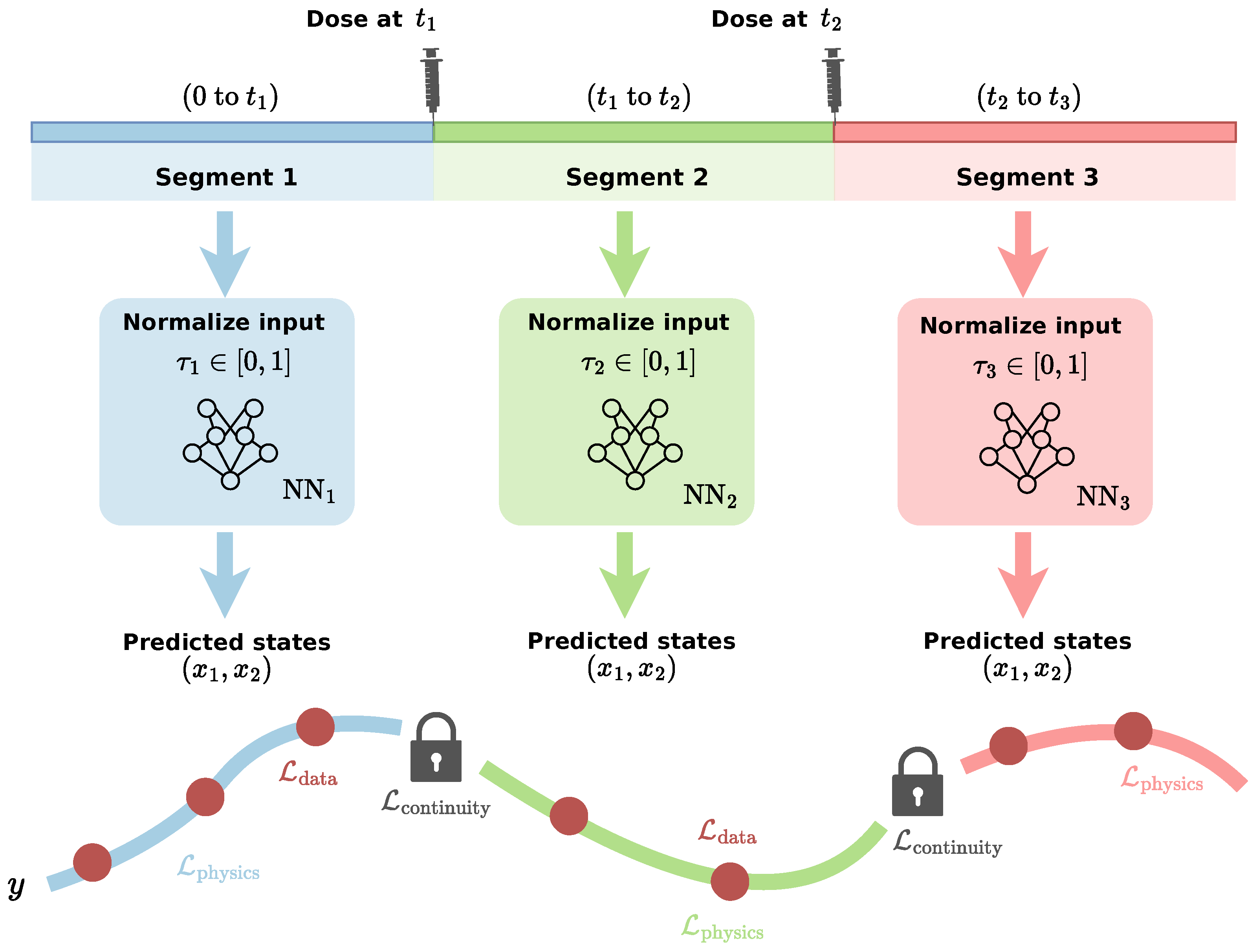
A schematic of the proposed Piecewise PINN architecture is presented in Figure 1 for two injections (the same structure can be used for an arbitrary number of injections). The diagram visualizes the workflow: first, the original time horizon is segmented based on dosing events to handle non-smooth dynamics. Within each segment, the time input is normalized to a local coordinate $\tau \in [0,1]$ to stabilize the training, where a separate independent neural subnetwork is trained for each time interval. Finally, the lower section of the diagram visualizes the model output (total tumor volume) derived from the state variables estimated by the neural networks. It illustrates how the distinct loss terms—detailed in Section 2.6—contribute to the reconstruction of the trajectory.

2.5. Analytic Representation of Dosing and Pharmacokinetics

Dose administrations are sharp transients in the drug exposure variables and, through the pharmacodynamic term, can produce rapid changes in the tumor dynamics also. In PINN, representing these effects by explicitly including the drug states $(x_3,x_4)$ as additional network outputs (as in our earlier work [40]) increases both the dimensionality of the approximation problem and the stiffness of the physics loss, because the network must simultaneously learn smooth tumor trajectories and fast drug kinetics across dosing events. Moreover, enforcing the pharmacokinetic equations with automatic differentiation requires computing additional derivatives and residual terms, which increases per-epoch cost.

In this paper, the pharmacokinetic subsystem (4) and (5) is linear in $(x_3,x_4)$ and is driven by impulsive inputs representing injections. Assuming the pharmacokinetic parameters c, $k_1$, and $k_2$ are known, the drug concentration $x_3$ in blood can be expressed in closed form as a sum of impulse responses. This removes the need to approximate $(x_3,x_4)$ with a neural network and to include an additional residual term during training. As a result, the PINN is trained using only the tumor states $(x_1,x_2)$, i.e., the measured tumor volume ($y=x_1+x_2$), while dosing effects are incorporated exactly through $x_3$ in the pharmacodynamic terms of (2) and (3).

Formally, we represent injections as instantaneous impulses; thus, the input at time t is given by

$$u\left(t\right)=\sum _{k=1}^K{u}_k\delta (t-t_k),$$

(10)

where $t_k$ and $u_k$ denote the time and dose of the k-th injection. Thus, between dosing events, the pharmacokinetic subsystem has no input and can be solved in closed form. Let

$${\lambda }_{1,2}={\displaystyle \frac{-(c+k_1+k_2)\pm \sqrt{{(c+k_1+k_2)}^2-4c{k}_2}}{2}},$$

(11)

be the eigenvalues of the system matrix of the PK subsystem (4) and (5) [9]; then, the impulse response is

$$w\left(\tau \right)={\displaystyle \frac{{\lambda }_1+k_2}{{\lambda }_1-{\lambda }_2}}{e}^{{\lambda }_1\tau }+{\displaystyle \frac{{\lambda }_2+k_2}{{\lambda }_2-{\lambda }_1}}{e}^{{\lambda }_2\tau },\tau \ge 0,$$

(12)

and $w\left(\tau \right)=0$, if $\tau <0$. The resulting drug concentration in the blood at time $t\ge 0$ is [9]

$$x_3\left(t\right)=\sum _{k=1}^K{u}_{k}w\left(t-t_k\right).$$

(13)

This analytical representation avoids numerically solving the $(x_3,x_4)$ subsystem during PINN training.

2.6. Piecewise PINN Formulation for Non-Smooth Dose Dynamics

Let $0<t_1<\cdots <t_K<T$ denote the dosing times on the horizon $[0,T]$. We assume that no dose is administered at $t=0$, and the total number of dose administrations is K. Dose injections induce sharp transients in the central-compartment drug level $x_3$ and, through the pharmacodynamic term, can also lead to rapid changes in the tumor dynamics. To capture this non-smooth behavior, we partition the time horizon into the dose-defined intervals

$$[0,t_1],[t_1,t_2],\dots ,[t_{K-1},t_K],[t_K,T],$$

(14)

i.e., we use the dosing times as internal segment boundaries. Here, $T>0$ denotes the final time of the study horizon, which in our experiments was set to a maximum of $T=105$ days. If the total tumor volume reached $2000{\mathrm{mm}}^3$ earlier, the mouse would have to be terminated due to animal welfare considerations; so, both the in vivo and in silico experiments stopped earlier.

On each interval $[t_k,t_{k+1}]$, we represent the tumor state trajectory using an independent neural subnetwork. Defining $t_0=0$ and $t_{K+1}=T$, we introduce a normalized local time coordinate

$$\tau \left(t\right)={\displaystyle \frac{t-t_k}{t_{k+1}-t_k}}\in [0,1],t\in [t_k,t_{k+1}],$$

(15)

which maps all subnetworks to a common input domain. This mapping places the input domain of every subnetwork on the same fixed range $[0,1]$. This standardization ensures uniform gradient scaling across segments with varying physical durations, preventing specific intervals from dominating the optimization, and improves numerical conditioning when computing time-derivatives via automatic differentiation.

The segment-wise network prediction is evaluated as a composition

$${\widehat{\mathbf{x}}}^{\left(k\right)}(t;\theta )={\widehat{\tilde{\mathbf{x}}}}^{\left(k\right)}\left(\tau \left(t\right);\theta \right),t\in [t_k,t_{k+1}],$$

(16)

where ${\widehat{\tilde{\mathbf{x}}}}^{\left(k\right)}(·;\theta )$ denotes the k-th subnetwork viewed as a function of $\tau \in [0,1]$.

In the physics loss, however, the residual is written in physical time t (original, not normalized) as in (7):

$$\mathbf{r}(t;\theta ,\alpha )={\partial }_t{\widehat{\mathbf{x}}}^{\left(k\right)}(t;\theta )-\mathbf{F}\left(t,{\widehat{\mathbf{x}}}^{\left(k\right)}(t;\theta );\mathbf{p}\left(\alpha \right)\right).$$

(17)

Automatic differentiation computes ${\partial }_t{\widehat{\mathbf{x}}}^{\left(k\right)}(t;\theta )$ by traversing the computation graph of the forward evaluation and systematically applying the chain rule. Since (16) is a composite mapping, autodiff applies the chain rule:

$${\partial }_t{\widehat{\mathbf{x}}}^{\left(k\right)}(t;\theta )={\partial }_{\tau }{\widehat{\tilde{\mathbf{x}}}}^{\left(k\right)}\left(\tau \left(t\right);\theta \right){\partial }_t\tau \left(t\right),$$

(18)

where $\tau \left(t\right)=(t-t_k)/\Delta t_k$ is linear in t on $[t_k,t_{k+1}]$, its derivative is constant:

$${\partial }_t\tau \left(t\right)={\displaystyle \frac{1}{\Delta t_k}}.$$

(19)

Thus, the factor $1/\Delta t_k$ enters the physical-time derivative automatically when gradients are taken with respect to t, as automatic differentiation applies the chain rule to the transformation from t to $\tau \left(t\right)$. Substituting (19) into (17) makes this explicit:

$$\mathbf{r}(t;\theta ,\alpha )={\displaystyle \frac{1}{\Delta t_k}}{\partial }_{\tau }{\widehat{\tilde{\mathbf{x}}}}^{\left(k\right)}\left(\tau \left(t\right);\theta \right)-\mathbf{F}\left(t,{\widehat{\tilde{\mathbf{x}}}}^{\left(k\right)}\left(\tau \left(t\right);\theta \right);\mathbf{p}\left(\alpha \right)\right).$$

(20)

Since the network is evaluated at the normalized local time $\tau \left(t\right)$ rather than at t directly, the derivative with respect to the physical time t is obtained by differentiating the network output with respect to $\tau$ and multiplying by ${\partial }_t\tau \left(t\right)=1/\Delta t_k$. This scaling is therefore included automatically by the differentiation procedure and ensures that the enforced residual corresponds to the correct physical-time ODE. Consequently, although the subnetworks are parameterized on $\tau \in [0,1]$, the enforced residual remains a correct physical-time ODE residual, and the parameters $\mathbf{p}$ retain their original physical interpretation and units (e.g., day⁻¹) without any manual rescaling.

Accordingly, the segment-wise state approximation is

$${\widehat{\mathbf{x}}}^{\left(k\right)}(t;\theta )=V\mathrm{softplus}\left({\mathrm{NN}}_{\theta }^{\left(k\right)}\left(\tau \left(t\right)\right)\right),t\in [t_k,t_{k+1}],$$

(21)

where ${\mathrm{NN}}_{\theta }^{\left(k\right)}:[0,1]\to {\mathbb{R}}^2$ denotes the k-th subnetwork with parameters $\theta$, and $\tau \left(t\right)$ is the normalized local time. The network outputs an unconstrained two-dimensional vector that is interpreted as the scaled tumor states on that segment. We apply the $\mathrm{softplus}$ activation elementwise,

$$\mathrm{softplus}\left(z\right)=log(1+e^z),$$

(22)

to enforce the physical constraint ${\widehat{x}}_1^{\left(k\right)}\left(t\right)\ge 0$ and ${\widehat{x}}_2^{\left(k\right)}\left(t\right)\ge 0$ for all t, while retaining differentiability everywhere (unlike using a hard constraint), which is advantageous when computing time-derivatives via automatic differentiation in the physics residual.

The multiplicative factor $V>0$ is a mouse-specific volume scale used to improve numerical conditioning. In our implementation, we set V as the maximum observed total tumor volume for the given mouse. It reduces the dynamic range of the data and physics losses, stabilizes gradient-based optimization, and makes the relative weighting between loss terms less sensitive to inter-mouse variation in absolute tumor volumes. After training, the predicted states are rescaled back to physical units by the factor V.

As our aim is to estimate the mathematical model parameters, we need constraints for those parameters to prevent them from going out of the unrealistic range. For example, the tumor proliferation rate has a lower and an upper biological limit. To enforce physiologically plausible bounds during training for the estimated model parameters, we optimize an unconstrained vector $\mathit{\alpha }\in {\mathbb{R}}^q$ and map it to the bounded parameter vector $\mathit{p}\in {\mathbb{R}}^q$ componentwise via a logistic transform. Let $p_i\in [p_i^{min}, p_i^{max}]$ denote the i-th parameter with prescribed bounds. We set

$$p_i\left({\alpha }_i\right)=p_i^{min}+\left(p_i^{max}-p_i^{min}\right)\sigma \left({\alpha }_i\right),i=1,\dots ,q,$$

(23)

where $\sigma \left(z\right)={\displaystyle \frac{1}{1+e^{-z}}}$ is the logistic sigmoid. This guarantees $p_i\left({\alpha }_i\right)\in [p_i^{min}, p_i^{max}]$ for all ${\alpha }_i\in \mathbb{R}$, while allowing unconstrained optimization in $\mathit{\alpha }$. In this study, we estimate only one model parameter at a time (either the proliferation rate a or the maximal drug effect parameter b) and treat all other parameters as fixed. It is important to note that the exact biological limits ($p_i^{min}$ and $p_i^{max}$) are not always known a priori in novel experimental settings. In this study, these boundaries were extracted from previous parameter estimation results based on the experimental cohort of 54 mice [9]. The applied parameter bounds for the estimation of the model parameters are summarized in

Table 2. Applied minimum and maximum values for the model parameters. These boundaries were extracted from previous parameter estimation results based on the experimental cohort of 54 mice.

Parameter	Minimum	Maximum	Unit
a	$0.0603$	$0.8147$	${\mathrm{day}}^{-1}$
b	$0.002368$	33	${\mathrm{day}}^{-1}$
n	$2.536\times {10}^{-5}$	$0.0461$	${\mathrm{day}}^{-1}$
w	$0.0704$	$0.0988$	${\mathrm{day}}^{-1}$
$E{D}_{50}$	$1.9256$	$2.3234$	$\mathrm{mg}·{\mathrm{kg}}^{-1}$
c	$1.8211$	$1.8211$	${\mathrm{day}}^{-1}$
$k_1$	$14.008$	$14.008$	${\mathrm{day}}^{-1}$
$k_2$	$136.2781$	$136.2781$	${\mathrm{day}}^{-1}$

.

2.7. The Parts of the Total Loss Function

Let ${\left\{(t_m,y_m)\right\}}_{m=1}^M$ denote the measurement points and ${\left\{t_i\right\}}_{i=1}^N$ the collocation points sampled uniformly within each segment. The training objective combines the data fit, physics consistency, initial conditions, and inter-segment continuity:

$$\mathcal{L}(\theta ,\alpha )=w_{\mathrm{data}}{\mathcal{L}}_{\mathrm{data}}+w_{\mathrm{phys}}{\mathcal{L}}_{\mathrm{phys}}+w_{\mathrm{ic}}{\mathcal{L}}_{\mathrm{ic}}+w_{\mathrm{cont}}{\mathcal{L}}_{\mathrm{cont}},$$

(24)

where $w_{\mathrm{data}}$, $w_{\mathrm{phys}}$, $w_{\mathrm{ic}}$, and $w_{\mathrm{cont}}$ are the corresponding weights that are set manually to balance the different magnitudes of the different terms in the composite loss function.

Optimization of $\mathcal{L}(\theta ,\alpha )$ is carried out using the Adam optimizer [45]. Separate learning rates are applied for the neural-network parameters ($\theta$) and the tumor-model parameter (a or b), reflecting their distinct roles in the optimization problem. For estimation of the tumor proliferation rate (a), the subnetworks and the parameter (a) are optimized jointly throughout training, using learning rates of $5\times {10}^{-4}$ for $\theta$ and ${10}^{-4}$ for a, respectively.

For the estimation of the maximal killing effect of the drug (b), a two-stage training procedure is applied. This training strategy is motivated by the structure of the tumor model equations. The parameter b enters the tumor dynamics through a nonlinear term coupling the tumor state to the drug concentration. Early during training, when the state approximation is inaccurate, the optimizer can reduce the physics residual by driving b toward artificially small values, effectively suppressing the drug-induced term and yielding physiologically implausible dynamics. To mitigate this effect, all model parameters are held fixed during an initial warm-up phase, and only the neural subnetworks are trained to solve the forward problem, using a learning rate of ${10}^{-3}$. Once a physically consistent state trajectory has been learned, the parameter b is released and optimized simultaneously with the subnetworks, using learning rates of $2\times {10}^{-4}$ for $\theta$ and ${10}^{-1}$ for b. This two-staged procedure reduces unfavorable optimization pathways and enables reliable estimation of the drug-effect parameter.

To ensure the reproducibility of our results, the complete neural network architecture and training hyperparameters are detailed in

Table 3. Neural network architecture and training hyperparameters applied for each piecewise segment.

Hyperparameter	Value
Number of hidden layers	3 (per segment subnetwork)
Nodes per hidden layer	32
Hidden activation function	Hyperbolic tangent (tanh)
Output activation function	Linear
Optimizer	Adam
Batch size	Full batch (evaluated segment-wise)
Collocation points	64 per segment

. The neural network and the training were implemented in Python v3.12.12 using the PyTorch v2.10.0 framework. The complete source code and the synthetic data generation pipeline are accessible in our public repository.

The loss-term weights used for estimation of the parameters a and b are summarized in

Table 4. Different weights of the loss terms used for parameter estimation of a and b.

Loss Term	Weights (Estimation of a)	Weights (Estimation of b)
Data misfit ($w_{\mathrm{data}}$)	20	10
Physics residual ($w_{\mathrm{phys}}$)	1	1
Continuity ($w_{\mathrm{cont}}$)	2	20
Initial condition ($w_{\mathrm{ic}}$)	1	10

. These values were selected empirically and kept fixed across all experiments.

It is important to emphasize that PINN performance is highly sensitive to the relative weighting of the distinct loss terms. The relative values in Table 4 were established empirically to balance the data misfit, the physics-based regularization, and the piecewise continuity constraints. During our experiments, we observed that varying these weight ranges leads to significantly different results. Specifically, an overly dominant data penalty ($w_{\mathrm{data}}$) causes the model to memorize noisy data points at the expense of physical consistency. On the other hand, when the physics penalty ($w_{\mathrm{phys}}$) dominates, the optimization process often suffers from gradient pathologies and collapses into trivial solutions [46,47]. By zeroing out the temporal derivatives, the network produces flat near-linear trajectories that strictly satisfy the differential equations but entirely disregard the empirical observations. Furthermore, if the continuity weight ($w_{\mathrm{cont}}$) is set too low, the piecewise architecture fails to align the states at the segment boundaries, producing non-physical jumps in the predicted volume at dosing events. The relative weightings detailed in Table 4 were specifically selected to mitigate these training pathologies, thereby yielding state trajectories that are smooth, dynamically plausible, and consistent with the observational data.

The data loss term minimizes the difference between the measured total tumor volume and the model-predicted total volume, obtained as the sum of the two predicted state variables.

$${\mathcal{L}}_{\mathrm{data}}={\displaystyle \frac{1}{M}}\sum _{m=1}^M{\left(\widehat{y}(t_m;\theta )-y_m\right)}^2,\widehat{y}(t;\theta )={\widehat{x}}_1(t;\theta )+{\widehat{x}}_2(t;\theta ).$$

(25)

Here, M is the number of measurement time points, $(t_m,y_m)$ denotes the m-th observation time and the corresponding measured tumor volume, ${\widehat{x}}_1(t;\theta )$ and ${\widehat{x}}_2(t;\theta )$ are the PINN-predicted state variables, and $\theta$ collects the neural-network parameters.

The physics loss term forces the PINN predicted state variables to satisfy the tumor growth ODE system. Using the PINN predictions ${\widehat{x}}_1(t;\theta )$ and ${\widehat{x}}_2(t;\theta )$ together with the analytically computed drug concentration $x_3\left(t\right)$, we form the ODE residuals as

$$\begin{array}{cc}\hfill r_1(t;\theta ,\alpha )=& {\partial }_t{\widehat{x}}_1(t;\theta )-\left[(a\left({\alpha }_1\right)-n){\widehat{x}}_1(t;\theta )-{\displaystyle \frac{b{\widehat{x}}_1(t;\theta )x_3\left(t\right)}{E{D}_{50}+x_3\left(t\right)}}\right],\hfill \end{array}$$

(26)

$$\begin{array}{cc}\hfill r_2(t;\theta ,\alpha )=& {\partial }_t{\widehat{x}}_2(t;\theta )-\left[n{\widehat{x}}_1(t;\theta )+{\displaystyle \frac{b{\widehat{x}}_1(t;\theta )x_3\left(t\right)}{E{D}_{50}+x_3\left(t\right)}}-w{\widehat{x}}_2(t;\theta )\right]\hfill \end{array}$$

(27)

where ${\partial }_t{\widehat{x}}_{\ell }(t;\theta )$ is computed by automatic differentiation, in the case when the estimated parameter is a, and

$$\begin{array}{cc}\hfill r_1(t;\theta ,\alpha )=& {\partial }_t{\widehat{x}}_1(t;\theta )-\left[(a-n){\widehat{x}}_1(t;\theta )-{\displaystyle \frac{b\left({\alpha }_2\right){\widehat{x}}_1(t;\theta )x_3\left(t\right)}{E{D}_{50}+x_3\left(t\right)}}\right],\hfill \end{array}$$

(28)

$$\begin{array}{cc}\hfill r_2(t;\theta ,\alpha )=& {\partial }_t{\widehat{x}}_2(t;\theta )-\left[n{\widehat{x}}_1(t;\theta )+{\displaystyle \frac{b\left({\alpha }_2\right){\widehat{x}}_1(t;\theta )x_3\left(t\right)}{E{D}_{50}+x_3\left(t\right)}}-w{\widehat{x}}_2(t;\theta )\right]\hfill \end{array}$$

(29)

in the case when the estimated parameter is b.

The trainable neural network parameters ${\alpha }_1$ and ${\alpha }_2$ enter only through $a\left({\alpha }_1\right)$ and $b\left({\alpha }_2\right)$, linking parameter inference to the requirement that the predicted states remain consistent with the mathematical model and the physiological constraints on the model (i.e., the limits).

Because the magnitude of the ODE terms scales with tumor size, we normalize the residuals by the predicted total volume $\widehat{y}(t;\theta )={\widehat{x}}_1(t;\theta )+{\widehat{x}}_2(t;\theta )$ to reduce the dominance of late time points with large volumes and to obtain a more balanced physics penalty along the trajectory. The resulting physics loss is

$${\mathcal{L}}_{\mathrm{phys}}={\displaystyle \frac{1}{N}}\sum _{i=1}^N\left[{\left({\displaystyle \frac{r_1(t_i;\theta ,\alpha )}{\widehat{y}(t_i;\theta )+1}}\right)}^2+{\left({\displaystyle \frac{r_2(t_i;\theta ,\alpha )}{\widehat{y}(t_i;\theta )+1}}\right)}^2\right],$$

(30)

where ${\left\{t_i\right\}}_{i=1}^N$ are collocation points sampled in the time domain, and $\alpha$ corresponds to ${\alpha }_1$ or ${\alpha }_2$, depending on which parameter is estimated.

We enforce the initial state at $t=0$ using the initial condition loss term. In the experiments, only the total tumor volume is available from the caliper measurement; so, we set the initial living tumor volume to this value and assume no necrotic volume initially, i.e., $x_{1,0}=y_0$ and $x_{2,0}=0$. The corresponding loss is

$${\mathcal{L}}_{\mathrm{ic}}={\left({\widehat{x}}_1(0;\theta )-y_0\right)}^2+{\left({\widehat{x}}_2(0;\theta )\right)}^2.$$

(31)

Since we use an independent subnetwork on each interval $[t_k,t_{k+1}]$, the segment-wise predictions may not be the same at the segment edges. To obtain a single continuous trajectory over $[0,T]$, we penalize mismatches of the predicted state at the internal boundaries given by the dosing times ${\left\{t_k\right\}}_{k=1}^K$ using the continuity loss term

$${\mathcal{L}}_{\mathrm{cont}}={\displaystyle \frac{1}{K}}\sum _{k=1}^K{∥{\widehat{\mathbf{x}}}^{(k-1)}(t_k;\theta )-{\widehat{\mathbf{x}}}^{\left(k\right)}(t_k;\theta )∥}_2^2.$$

(32)

This term enforces continuity by aligning the left- and right-segment state predictions at each dosing time.

2.8. Synthetic Data Generation

To evaluate the PINN-based parameter estimation, we generated synthetic datasets that closely mimic the structure of the in vivo mouse experiments while retaining known ground-truth parameters. This enables the systematic assessment of the estimation accuracy under realistic dosing schedules. We used a previously recorded dosing schedule for each mouse, extracted from the applied treatment protocol during the mouse experiments, and treated them as fixed inputs.

For each mouse, the tumor growth model was simulated over a horizon of $T=105$ days or terminated earlier if the total tumor volume reached 2000 mm³, reflecting experimental endpoints in cases of uncontrolled tumor growth. The full system was solved numerically on a uniform grid with 10 time steps per day (i.e., 1050 points over 105 days) to generate reference trajectories for the living and dead tumor volumes, $(x_1,x_2)$, and the total tumor volume ($y=x_1+x_2$). Dose administrations were incorporated as impulsive inputs in the pharmacokinetic subsystem, with the described analytical solution above in Equation (13).

In order to simulate realistic experimental observations, synthetic tumor volume measurements were generated by sampling the total tumor volume at discrete measurement times matching the experimental schedule (i.e., three times a week: Monday, Wednesday, and Friday). Further, additive Gaussian noise was applied to each measurement,

$$y_m^{\mathrm{obs}}=y\left(t_m\right)+{\eta }_m,{\eta }_m\sim \mathcal{N}\left(0,0.05\overline{y}\right),$$

(33)

where $\overline{y}$ denotes the mean tumor volume for the given mouse. Negative values were clipped to ensure non-negativity, reflecting the measurement limitations. This simple noise model is introduced solely to insert baseline measurement variability into the synthetic data and to demonstrate the general robustness of the PINN architecture. To evaluate the effect of noise variance, we conducted sensitivity tests by increasing the noise scale from the baseline 5% up to 60%. Our results show that the PINN is robust to this type of Gaussian noise: for a ground-truth parameter $b=13.11$, the relative estimation errors remained below 5% for noise levels up to 40% (specifically 2.90%, 4.81%, and 2.06% for the 5%, 20%, and 40% noise cases, respectively). Even under extreme conditions with 60% noise variance, the estimation error remained within 11.90%, demonstrating that the physics-informed regularization effectively compensates for high observational uncertainty. However, in actual preclinical settings, digital caliper measurements contain structurally more complex volume-dependent errors. Therefore, replacing this with a more realistic noise model based on paired MRI and caliper data [25] to evaluate the robustness of the PINN under true experimental uncertainty remains a primary focus for our future work.

This procedure was repeated for all 54 mice, yielding a collection of synthetic datasets consisting of tumor volume observations, original state variables and corresponding dosing schedules and model parameters. This generated dataset was used for PINN training and evaluation, allowing direct comparison between the estimated and true parameters.

3. Results

3.1. State Variables Reconstruction

We evaluated the accuracy of the proposed PINN in reconstructing state variables on the generated mouse datasets with known ground-truth parameters and dosing schedules. During training, only the total tumor volume was provided as observational data, i.e., $y=x_1+x_2$, while the living and dead tumor volumes $x_1$ and $x_2$ were not directly supervised. Therefore, an important part of the evaluation was to verify that the PINN not only reproduces y but also recovers a state decomposition $(x_1,x_2)$ that is consistent with the ground-truth composition.

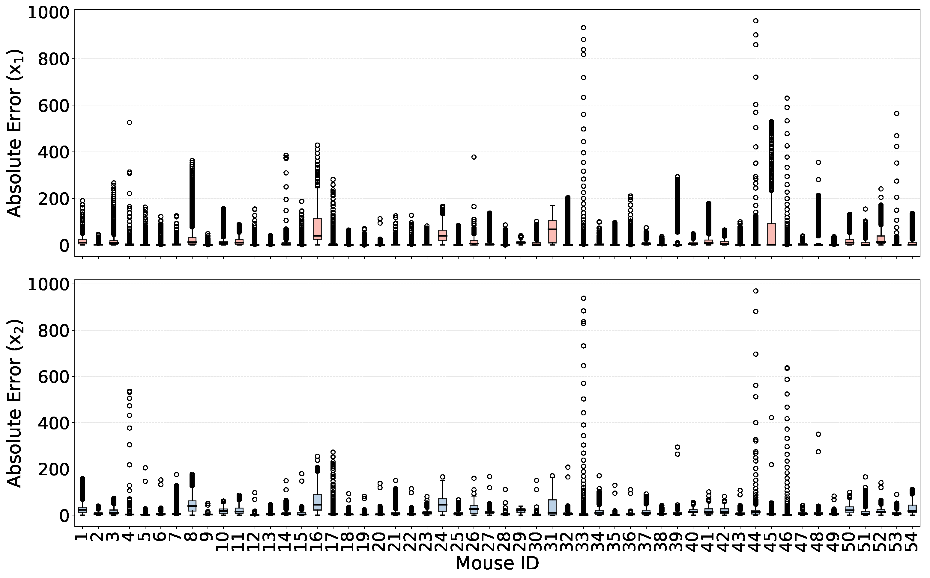
Figure 2 summarizes the absolute reconstruction error for the living ($x_1$) and dead ($x_2$) tumor volumes across all the mice using boxplots for the case of the estimation of parameter a. Each box corresponds to one mouse and consists of the absolute errors over the simulated time horizon. The absolute error is calculated as the difference between the original state variable and the predicted state variable by PINN. The results show low median errors for most mice, indicating that the PINN can infer the unobserved state decomposition from total tumor-volume measurements and the imposed physical constraints. Outliers are observed in a subset of cases, typically associated with rapidly changing dynamics.

Table 5. Summary of the reconstruction error (Median of the Absolute Error—MedAE) for the 54 mice.

Metric	Population Mean	Population Median	Range [Min, Max]
MedAE ($x_1$)	4.26	0.50	[0.00, 40.38]
MedAE ($x_2$)	10.17	6.01	[0.90, 45.57]
MedAE (y)	12.65	6.76	[1.04, 78.66]

reports the Median of the Absolute Error (MedAE) for the state variables $x_1$ and $x_2$ across the simulated mouse dataset. Both compartments exhibit small mean and median MedAE values ($4.26$, $10.17$, $0.50$, and $6.01$), indicating accurate state reconstruction on average. While some of the mice show larger error values, the observed maxima remain within an acceptable range.

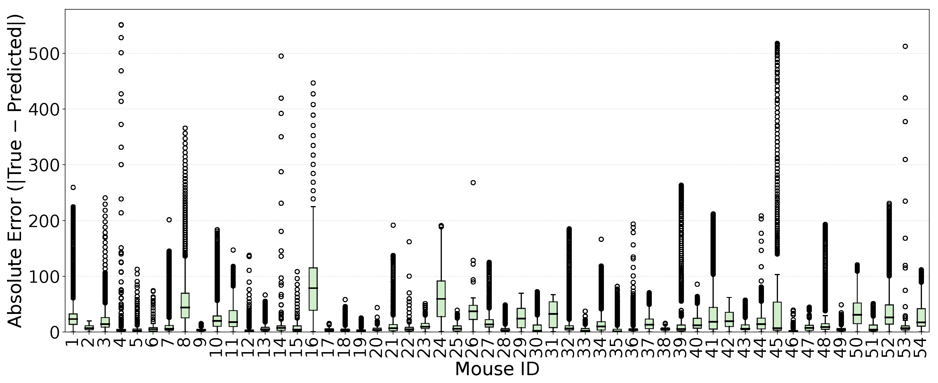
In order to assess predictive performance at the observable level, Figure 3 presents boxplots of the absolute error between the true and predicted total tumor volume. Since the data-misfit term directly constrains only the observable $y=x_1+x_2$, the PINN is explicitly optimized to reproduce the measured tumor volume, whereas the individual compartments $(x_1,x_2)$ are recovered indirectly through the physics constraints. Consistent with this, total-volume errors remain low across most mice, indicating accurate reconstruction of y.

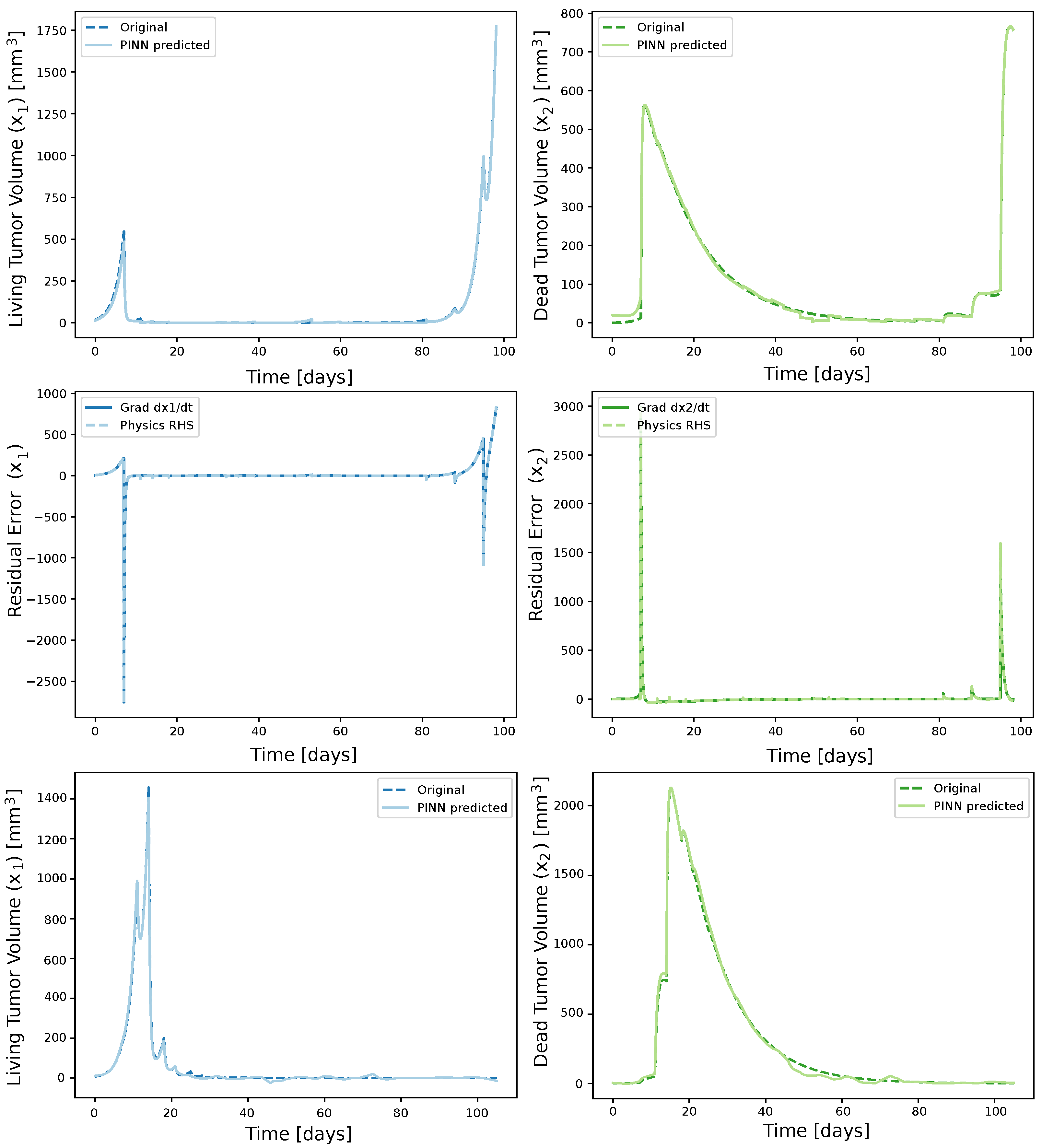
Figure 4 presents two representative examples from the cohort of 54 mice. The first row corresponds to estimation of the tumor proliferation rate (a), while the third row illustrates estimation of the maximal drug killing effect parameter (b). In both cases, the PINN accurately reconstructs the living ($x_1$) and dead ($x_2$) tumor volumes, with predicted trajectories closely matching the noiseless reference solutions over the full simulation horizon. The figures in the second row show the physics-based residuals defined in (26) and (27) for the estimation of parameter a at the end of training, demonstrating consistency between the learned trajectories and the governing tumor-dynamics model.

3.2. Parameter Inference

For each mouse, the model parameters were obtained from previously estimated values [9,11]. The estimation in the present study focused on the tumor proliferation rate a and the maximal drug-effect parameter b. They were estimated separately, and all remaining model parameters were kept fixed throughout the analysis. These included tumor and pharmacodynamic parameters (n, w and $E{D}_{50}$), which were taken from previously reported estimates, as well as the pharmacokinetic parameters $(c,k_1,k_2)$. The pharmacokinetic parameters were obtained from independent measurements and treated as identical across the cohort. This choice was motivated by identifiability and optimization stability: when simultaneously estimating multiple parameters together with latent state trajectories under partial observability (total volume only), the training objective convergence was unreliable in this PINN setting. We therefore restricted learning to the most identifiable parameters, a and b, and treated the remaining parameters as fixed across all simulations.

Figure 5 and

Table 6. Estimation accuracy for the tumor growth rate parameter (a).

Metric	Population Mean	Population Median	Range [Min, Max]
Absolute Error (a)	0.033	0.02	[0.0001, 0.16]
Percentage Error (a)	7.12%	5.51%	[0.02%, 32.19%]

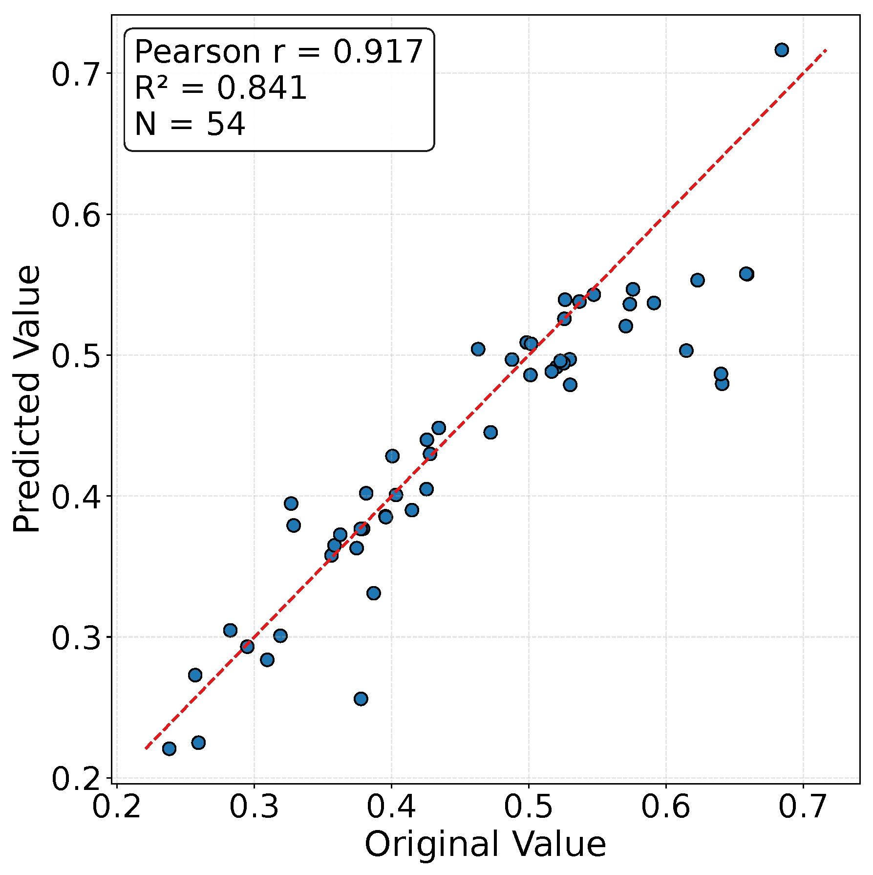
summarize the accuracy of the estimated tumor growth parameter (a) across the full generated in silico cohort. Figure 5 compares the PINN-estimated values of a with the corresponding ground-truth values used to generate the synthetic datasets, showing a strong agreement across mice. Most estimates lie close to the identity line, indicating reliable recovery of the true parameter values under partial observability. We can also say that the main difference is in the case of larger parameter values. The closeness between the estimated and ground-truth values of the tumor growth parameter a is further quantified by the coefficient of determination, $R^2$. In Figure 5, the reported value $R^2=0.841$ indicates a strong linear relationship between the predicted and true parameters and supports the robustness of the proposed parameter-estimation approach.

Figure 4. Example state reconstruction for two representative mice. The top and bottom rows show reconstruction results for the estimation of parameters a and b, respectively. The middle row figures display the corresponding physics-based residuals for the estimation of parameter a.

Figure 4. Example state reconstruction for two representative mice. The top and bottom rows show reconstruction results for the estimation of parameters a and b, respectively. The middle row figures display the corresponding physics-based residuals for the estimation of parameter a.

Table 6 complements this visual assessment by reporting summary statistics of the estimation error for parameter a across all mice. The low mean and median error confirms that accurate parameter identification is achieved for the majority of subjects, while the spread captured by the minimum and maximum of the errors shows only $32.19$% error in the worst case also. Together, Figure 5 and Table 6 demonstrate that the proposed PINN framework can robustly infer the proliferation rate across the 54 mice.

Figure 5. Comparison of PINN-estimated parameter (a) with the ground-truth values used to generate the synthetic datasets for all 54 mice. The blue dots represent individual subjects, and the red dashed line is the identity indicating perfect agreement between the estimated and original values. The high coefficient of determination ($R^2=0.841$) demonstrates reliable parameter estimation in most cases.

Figure 5. Comparison of PINN-estimated parameter (a) with the ground-truth values used to generate the synthetic datasets for all 54 mice. The blue dots represent individual subjects, and the red dashed line is the identity indicating perfect agreement between the estimated and original values. The high coefficient of determination ($R^2=0.841$) demonstrates reliable parameter estimation in most cases.

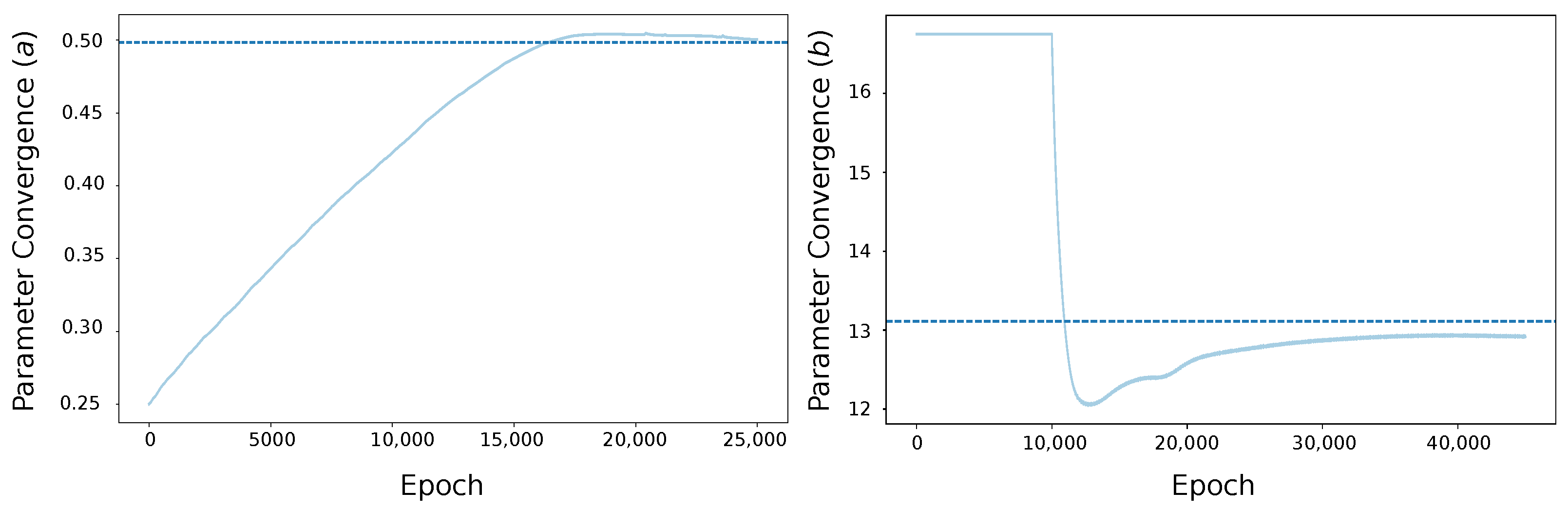
While Figure 5 and Table 6 summarize the accuracy of the parameter estimation in the whole generated dataset, Figure 6 illustrates the parameter convergence for the two example mice shown in Figure 4. The figure on the left shows how the estimated proliferation rate a reaches a stable value as training progresses, around the 18,000th epoch. The dashed line shows the original (ground-truth) value of the parameter. In the right figure, the temporal evolution of the estimated parameter b is shown. During the first 10,000 epochs, b is held fixed (on its initial value, the mean of the interval) while the network learns a forward solution, leading to convergence of the predicted states toward the reference trajectories. In the subsequent 35,000 epochs, b is released and simultaneously optimized with the subnetworks’ weights, converging toward its true value. Overall, this example demonstrates stable convergence and indicates that accurate parameter estimation is achieved through the combined effects of data fidelity and physics-based regularization. Training was performed using an NVIDIA T4 GPU and required approximately 176 min for 35,000 epochs for this mouse.

When estimating multiple parameters simultaneously, training was more sensitive to non-unique solutions. In particular, the optimizer could reduce b to unrealistically small values, effectively weakening and smoothing the dose-induced response, and then compensate by also decreasing a. This behavior indicates limited identifiability under the current architecture and loss weighting: multiple parameter combinations could match similar observations, even if some combinations are not physiologically plausible.

In addition, the method has not yet been validated on real measurements, where biological processes not represented in the model (e.g., resistant subpopulations) can influence the observed dynamics. In such settings, the PINN may absorb unmodeled effects into the inferred parameters. For example, resistant phases may be fitted by increasing a while decreasing b relative to nominal values. Future work should therefore aim to detect and appropriately treat time intervals that are not well explained by the current mechanistic model and, where necessary, extend the mathematical formulation to capture additional biological phenomena.

Overall, the single-parameter experiments demonstrate that the proposed framework can robustly recover the dominant tumor growth rate a and the maximal effect of drug parameter b in the presence of impulsive dosing. Extending this approach to reliable multi-parameter estimation will require architectural and methodological refinements, including stronger identifiability constraints and mechanisms to separate model-consistent dynamics from unmodeled biological behavior.

3.3. ODE Reconstruction

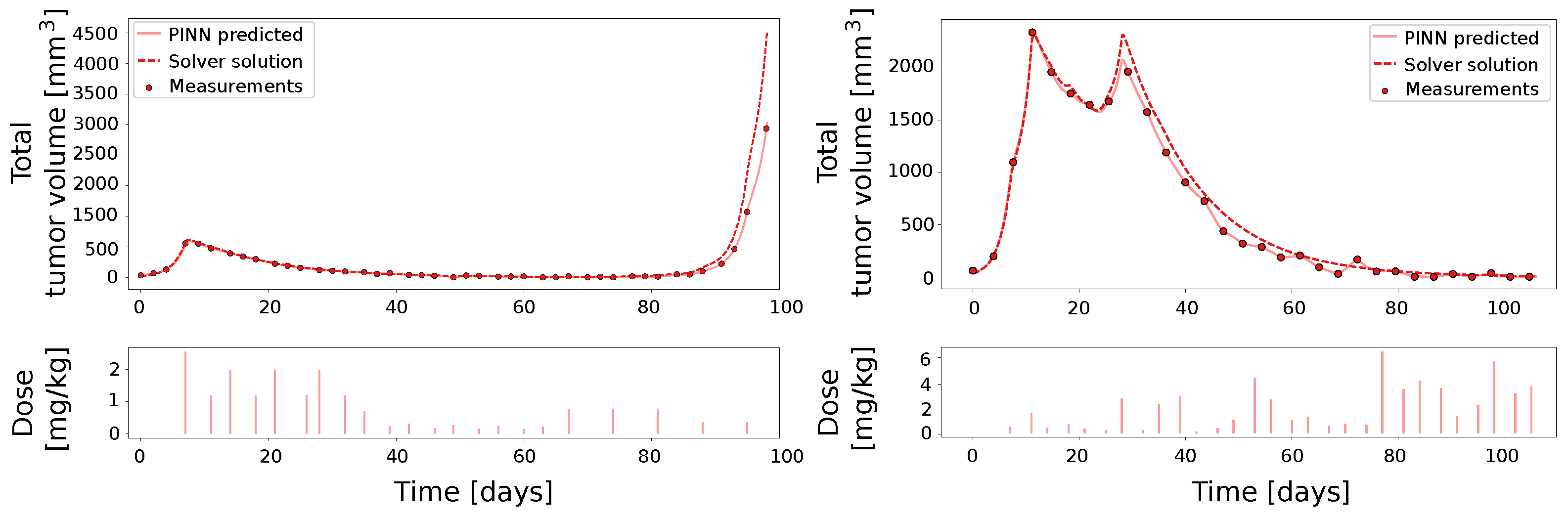
To further validate the inferred parameters, Figure 7 compares the PINN-predicted total tumor volume with an ODE numerical solver simulation in the two selected mice cases visualized in Figure 4 and Figure 6. The ODE trajectories are generated using the parameter values estimated by the PINN and are computed with the LSODA solver from the SciPy library (v1.16.3). The PINN predictions and the ODE solver trajectories agree closely over the full simulation horizon, with the main discrepancy appearing in the final phase of rapid growth in the left figure, indicating that the estimated parameter is broadly consistent with the underlying tumor dynamics.

Minor discrepancies between the PINN predictions and the ODE-based solutions may occur for several reasons. This behavior reflects the fact that the PINN is trained by minimizing a weighted composite loss comprising data-fit, physics-residual, initial-condition, and continuity terms, rather than enforcing the governing ODE exactly at every time point. In particular, as illustrated in the right panel, the PINN trajectory places stronger emphasis on matching the data points, suggesting that the relative weighting between the data and physics loss terms could be further adjusted to reduce these deviations. Additional differences can arise from numerical factors, such as using different time grids for evaluating the PINN and solving the ODE, and from implementation details related to non-smooth dosing inputs and non-negativity constraints. Moreover, the underlying tumor growth model can be sensitive to small variations in parameter values, particularly during phases of rapid tumor growth; so, even minor differences in the estimated parameters may lead to visibly diverging trajectories over time.

Table 7. ODE solution errors in mm³ by using the PINN-predicted parameters across the in silico dataset.

Metric	Population Mean	Population Median	Range [Min, Max]
Mean ODE Err	17.48	12.01	[2.61, 82.51]
Median ODE Err	12.65	6.76	[1.04, 78.66]

summarizes the consistency across the full dataset of 54 mice for the case of estimation the parameter a. For each mouse, we computed the pointwise absolute difference between the PINN-predicted and ODE-simulated total tumor volumes on the same time grid and then summarized these errors over time by their mean and median. The population mean (or median) was then computed as the mean (or median) of the corresponding per-mouse summaries across the 54 mice.

Relative to the typical tumor burden in the synthetic cohort (global mean $417.41$ and median $272.83$ mm³), the ODE–PINN discrepancies are small. The population mean of the per-mouse mean ODE error is $17.48$ mm³, corresponding to $4.19\%$ of the global mean, while its population median is $12.01$ mm³ ($4.40\%$ of the global median). Similarly, the population mean of the per-mouse median ODE error is $12.65$ mm³ ($3.03\%$ of the global mean), and its population median is $6.76$ mm³ ($2.48\%$ of the global median). Overall, this suggests that ODE simulations using the PINN-estimated parameters typically remain within a few percent of the tumor volumes, with larger mismatches confined to a small subset of outlier cases (maximum errors up to $82.51$ mm³).

4. Discussion

This study evaluated a PINN framework for parameter inference in a deterministic tumor model under a realistic observation setting, where only the total tumor volume is measured. Using controlled in silico experiments, we assessed whether such partial observability still permits reliable recovery of model dynamics and key parameters. To handle the non-smooth dynamics induced by impulsive drug dosing, we employed a piecewise PINN formulation, which allowed stable training across repeated dosing events. This approach accurately reproduced the observed total tumor volume across a cohort of 54 mice and, despite indirect supervision, reconstructed latent state trajectories $(x_1,x_2)$ with a low reconstruction error.

Focusing on parameter inference, we restricted estimation to the tumor proliferation rate a and the maximal drug killing effect parameter b, which prior sensitivity and identifiability analyses identified as the most reliably informed parameters under limited observability [33,48]. The method was evaluated across the cohort for the estimation case of parameter a, where the PINN recovered a with high accuracy, as evidenced by the strong correlation between inferred and ground-truth values ($R^2=0.841$). Importantly, forward simulations performed with a conventional ODE solver using the PINN-estimated parameters closely matched the learned trajectories.

A key practical advantage of the proposed approach is that it embeds the mechanistic ODE structure directly into the training objective via automatic differentiation, thereby reducing the reliance on repeatedly solving the full ODE system inside an outer-loop optimizer. In practice, in the case of this specific tumor model, this formulation worked reliably for single-parameter estimation, where the physics constraints and data terms were sufficient to identify the target parameter.

At the same time, these conclusions should be interpreted in light of several practical limitations. First, the main evaluation was performed on synthetic trajectories generated by the same mechanistic model that is enforced during training. While this controlled setup enables quantitative validation of reconstruction and parameter identification, it does not capture the model mismatch and biological heterogeneity expected in real measurements, such as resistant subpopulations or other unmodeled effects. Consistent with this, preliminary experiments on more complex or mismatched dynamics indicated that the PINN can absorb unmodeled behavior into parameter estimates (e.g., increasing a while suppressing drug-related effects), which motivates explicit mechanisms to detect and treat model-incompatible intervals or to extend the mechanistic model when needed.

Second, restricting inference to a single parameter (a and b) was essential for stable optimization, but it also limits applicability when additional parameters must be inferred from sparse total-volume observations. In preliminary multi-parameter runs, the optimization admitted numerically convenient trade-offs, for instance, driving b (maximal effect of drug) to unrealistically low values to reduce the need to represent sharp drug-induced transients, which indicates limited identifiability under the current loss weighting and architecture. Third, the training outcome depends on practical choices such as loss weights, collocation density, initialization, and the relative emphasis of data fit versus physics regularization.

These observations suggest several directions for future work. Improving the robustness of multi-parameter inference will likely require stronger priors or identifiability constraints, as well as adaptive strategies for balancing loss terms. For real-data applications, the workflow should incorporate methods to identify and appropriately handle time intervals that are not well explained by the current mechanistic model. Incorporating more realistic observation models (including more realistic noise) and leveraging additional data modalities would further improve the model. From a runtime perspective, improved domain-decomposition strategies and parallelization could reduce the training time for long horizons and dense dosing schedules. Together, these extensions would move the approach closer to reliable parameter inference and mechanistic reconstruction on experimental mouse measurements.

5. Conclusions

This work introduces a piecewise PINN for parameter inference in a mechanistic tumor model when only the total tumor volume is observed. The loss combines data fit with ODE residual terms and continuity constraints at dosing times. On synthetic data from 54 mice, the method reconstructed the total tumor volume accurately and recovered the original latent states. Estimating only the proliferation rate (a) or the maximal effect of drug (b) resulted in precise mouse-specific values and stable training. We further validated the estimates by running an independent ODE solver with the PINN-inferred parameters. The forward simulations closely matched the PINN trajectories, supporting the consistency. These results suggest that PINNs can replace classical outer-loop optimization for dose-driven tumor models, especially with sparse measurements and latent states. Future work will extend the method to stable multi-parameter estimation and test it on real measurements. This will require improved identifiability, explicit handling of model mismatch, and uncertainty quantification.