Fréchet Distance-Based Vehicle Selection and Satisfaction-Aware Vehicle Allocation for Demand-Responsive Shared Mobility: A Discrete Event Simulation Study

Abstract

Demand-responsive transit (DRT) requires real-time vehicle assignment under dynamically arriving requests, where each decision may alter multi-stop routes and affect both onboard and newly arriving passengers. However, DRT simulations often face three key limitations: rapidly increasing computational complexity as fleet size and demand grow, insufficient integration of traffic congestion into routing decisions, and limited consideration of passenger-oriented service quality in final vehicle assignment. To address these issues, this study proposes an integrated DRT simulation incorporating three core algorithms: Fréchet Distance-based Candidate Vehicle Selection (FD-CVS), Congestion-Aware Path Planning (CA-PP), and Satisfaction-Aware Vehicle Assignment (SA-VA). FD-CVS reduces computational burden by filtering candidate vehicles based on route similarity. CA-PP extends conventional path planning by incorporating congestion-adjusted travel costs derived from public transportation data. SA-VA determines the final vehicle assignment by jointly evaluating passenger waiting time, in-vehicle travel time, and capacity constraints. The algorithms are implemented within a discrete-event simulation environment using real-world data. Experimental results demonstrate that FD-CVS significantly reduces execution time under high-demand conditions, while SA-VA improves passenger waiting time and acceptance rates. Overall, the proposed three-algorithm framework enables more realistic and computationally efficient DRT system evaluation.

1. Introduction

1.1. Research Background and Motivation

Demand-responsive transit (DRT) has gained increasing attention as a flexible alternative to fixed-route public transportation systems, particularly in suburban and rural areas with low demand density [1,2,3]. Unlike conventional public transport operating on predetermined routes and schedules, DRT dynamically adjusts vehicle routes and assignments in response to real-time passenger requests. This operational flexibility allows service providers to better accommodate temporal and spatial demand variations while potentially improving service efficiency.

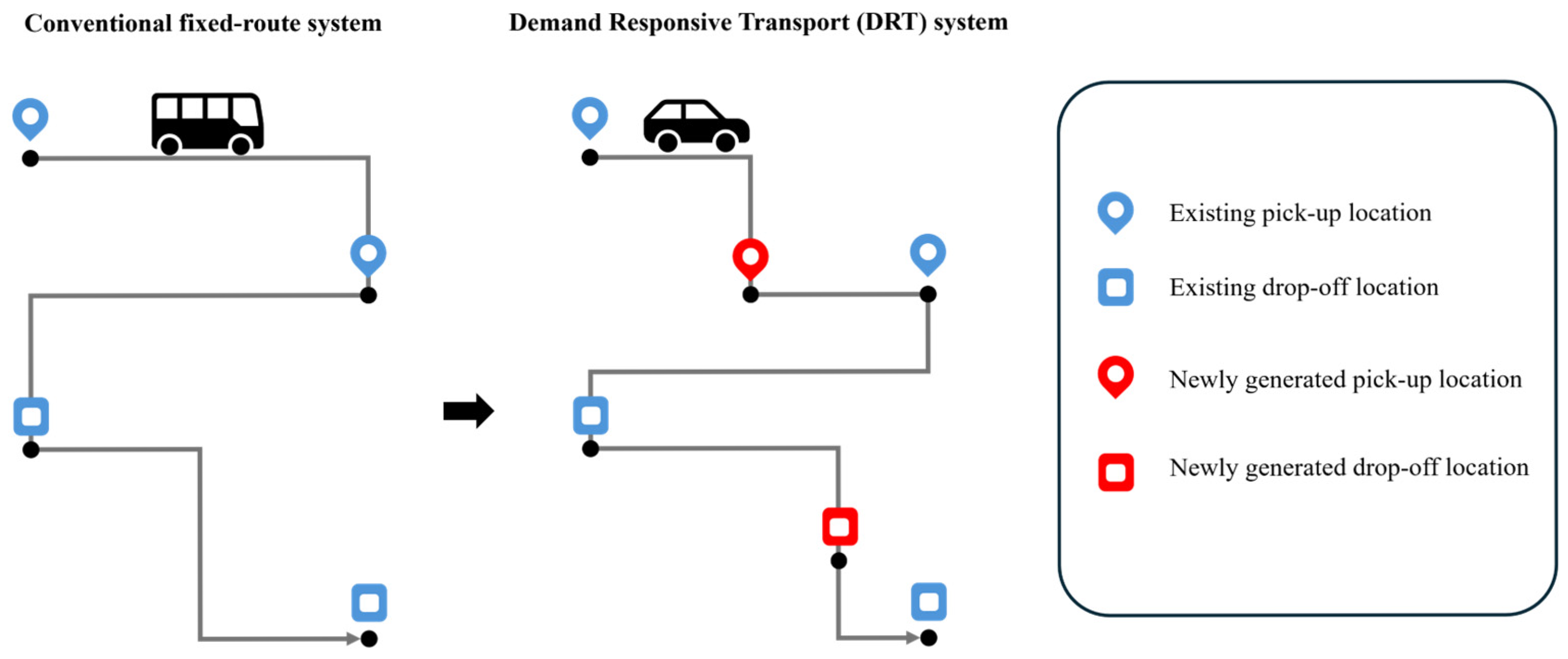
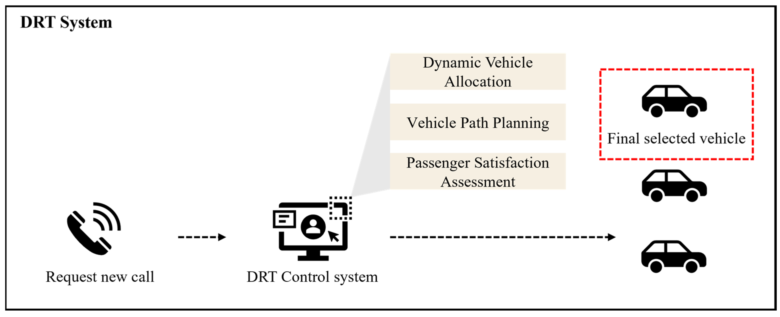
Figure 1 illustrates the fundamental differences between conventional fixed-route transportation and the target DRT system. While traditional systems rely on static routes and schedules, DRT continuously updates vehicle movements based on incoming passenger requests. In the figure, the blue nodes represent the predefined fixed routes of the conventional system, whereas the red nodes denote dynamically generated nodes created in response to passenger requests. This dynamic nature enhances adaptability but also increases operational complexity [4]. Figure 2 summarizes a typical DRT operating cycle consisting of three stages: (i) passenger request generation, (ii) candidate route generation and vehicle assignment, and (iii) final service execution. Importantly, the core operational challenge is vehicle assignment under dynamic requests, because DRT vehicles can serve multiple passengers simultaneously and a single assignment decision may affect the waiting and riding times of both onboard passengers and newly arriving passengers [5,6]. Thus, in DRT, route planning should be understood as an integral part of assignment evaluation rather than as an independent objective.

Despite these advantages, simulation-based evaluation of DRT operations faces significant challenges. First, as fleet size and demand increase, the number of possible vehicle–request combinations grows rapidly, leading to substantial computational burden [7,8,9]. Next, realistic DRT evaluation requires consideration of traffic conditions and passenger-oriented service metrics such as waiting time and riding time [10,11,12,13,14,15,16]. If these elements are not properly integrated, simulation results may fail to reflect actual operational behavior. Therefore, there remains a need for a unified simulation framework that simultaneously improves computational scalability, congestion-aware routing, and passenger-oriented assignment [17,18,19].

To address this issue, this study proposes a DEVS-based DRT simulation framework incorporating three complementary algorithms: Fréchet Distance-based Candidate Vehicle Selection (FD-CVS), Congestion-Aware Path Planning (CA-PP), and Satisfaction-Aware Vehicle Assignment (SA-VA). By integrating route similarity-based candidate filtering, congestion-adjusted path planning, and satisfaction-driven vehicle assignment within a single simulation environment, the proposed framework enables a more realistic and computationally efficient evaluation of large-scale DRT systems.

1.2. Related Works

DRT systems require dynamic route planning to accommodate heterogeneous passenger requests with continuously changing origins and destinations. Because routes are frequently modified in real time, dispatching decisions must simultaneously consider onboard passengers, newly arriving requests, and traffic conditions. As demand increases, computational complexity grows rapidly, posing a major challenge for real-time system operation (

Table 1. Comparison of simulation studies on DRT systems.

Related Research	Passenger Satisfaction	Traffic Congestion Incorporation	Candidate Vehicle Selection	Key Limitation
Zigrand et al. (2024) [20]	X	X	X	Assumes future requests at service start
Park et al. (2023) [21]	X	X	X	Focuses on demand heterogeneity, without explicitly addressing passenger satisfaction, traffic-aware routing, or candidate vehicle selection
Wu et al. (2025) [22]	X	O	X	Uses synthetic rather than real traffic data
Han et al. (2024) [23]	O	X	X	Assumes equal delay times instead of reflecting real conditions
Dastani et al. (2024) [24]	△	X	O	Interprets satisfaction as preference grouping rather than service quality
Lu et al. (2022) [25]	O	O	X	Only predefined request sets accepted; no new request arrivals considered
Ghandeharioun & Kouvelas (2023) [26]	O	O	△	Candidate set limited to nearest vehicles; no guarantee of optimal assignment
Cho et al. (2025) [27]	O	△	X	No route similarity-based filtering; limited congestion integration; computational scalability not addressed
Our method	O	O	O	Computational efficiency is improved by restricting candidate vehicles, but global optimality is not guaranteed

Note: O denotes that the corresponding issue is fully addressed in the paper; △ denotes partial or limited consideration; X denotes that the issue is not addressed.

).

Several studies have addressed route optimization for DRT systems using mathematical programming and stochastic formulations. Earlier work formulated DRT routing problems based on predefined or probabilistic request sets to optimize route structures and reduce computational time [20,25]. More recently, time-dependent traffic conditions have been incorporated into real-time insertion models using mixed-integer linear programming (MILP) formulations [22]. Although these approaches improve routing efficiency under specific assumptions, they do not explicitly account for passenger satisfaction or candidate vehicle selection, and their computational scalability and real-time applicability remain limited. Recent studies have further expanded this line of research by considering heterogeneous demand and congestion-sensitive transportation decision making. For example, Park et al. investigated on-demand mobility service optimization under spatial heterogeneity in travel demand, highlighting the importance of demand distribution in service design and operational efficiency [21]. In addition, Obonguta et al. addressed congestion-related route choice and user-cost minimization in a road network setting, emphasizing the role of stochastic user equilibrium and iterative solution methods in solving complex transportation problems. These studies suggest that, as the number of operational variables and traffic-related factors increases, computational complexity becomes a critical issue in transportation system design [28].

Another line of research emphasizes passenger satisfaction by introducing delay tolerance and preference-based modeling approaches. Passenger-specific delay thresholds have been used to balance service quality and operator revenue [23], whereas preference-based matching mechanisms have been proposed to improve perceived service quality [24]. However, these studies do not explicitly integrate traffic conditions and primarily focus on satisfaction from a modeling perspective rather than on operational efficiency.

More recently, traffic-aware routing approaches have been developed to improve the realism of DRT operations. Real-time congestion information has been incorporated into route planning, and candidate vehicles have been restricted to nearby fleets to reduce computational complexity [26]. While effective in improving responsiveness, such heuristic candidate selection strategies do not guarantee global optimality.

Cho et al. developed a DEVS-based simulation framework for analyzing DRT operations under dynamic passenger demand [27]. While the framework provided a structured discrete-event modeling environment for operational evaluation, it did not incorporate route similarity-based candidate filtering or a fully integrated congestion-aware path planning mechanism. Consequently, computational scalability and the interaction between congestion and vehicle assignment remained insufficiently addressed.

Overall, existing DRT studies typically address only a subset of the three critical factors: passenger satisfaction, candidate vehicle selection, and integration of traffic conditions. In contrast, the present study proposes an integrated framework that simultaneously considers all three aspects within a Discrete Event System Specification (DEVS)-based simulation environment. Specifically, the proposed framework improves computational efficiency by reducing the candidate vehicle set through Fréchet distance-based vehicle selection, while also enhancing service quality through satisfaction-aware passenger insertion and traffic-aware routing under real-time DRT conditions.

2. Materials and Methods

2.1. Proposed Process Approach

This section describes the overall architecture of the proposed simulation framework for implementing a DRT system. Because DRT operations are driven by discrete events such as passenger requests, a discrete-event simulation approach is adopted. Rather than relying on an off-the-shelf simulation tool, the framework is implemented using a formal modeling methodology to effectively represent the system’s complex structure [29]. To enhance realism, the simulation model is constructed using real public transportation data to predict passenger demand and traffic conditions and to support the generation of dynamic nodes.

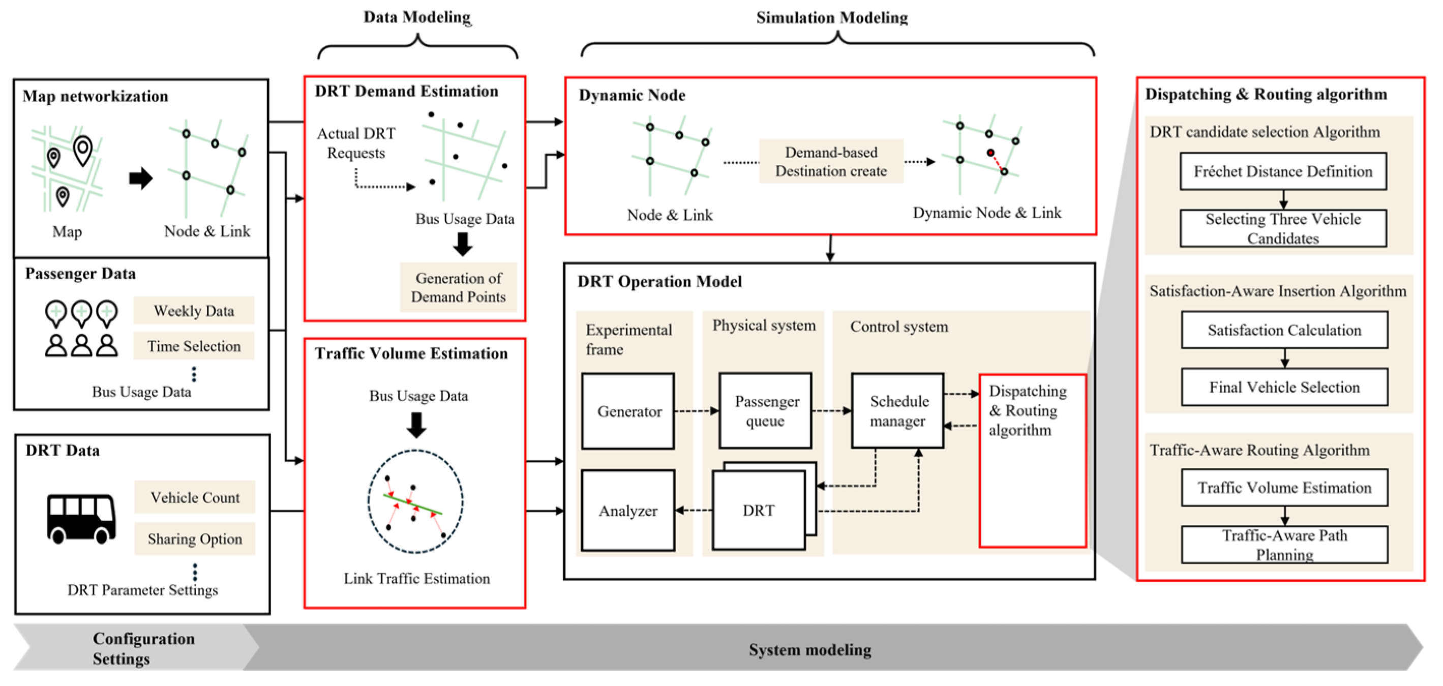
The overall structure of the proposed framework is illustrated in Figure 3. The framework is divided into two main stages: (1) simulation environment configuration and (2) system modeling. In the first stage, the simulation environment is configured by defining the map data, DRT operational data, and passenger-related data required for execution. These datasets are derived from real-world geographic and demand information corresponding to the target study area and are preprocessed into formats suitable for simulation. The second stage (system modeling) is further divided into data modeling and simulation model implementation. Data modeling focuses on preprocessing the configured datasets to enable realistic simulation behavior [30]. Rather than using synthetically generated inputs, actual DRT request volumes and day-of-week public transportation usage data are employed to estimate passenger demand. In addition, public transportation usage data are transformed into regional traffic volume indicators to estimate road-level congestion.

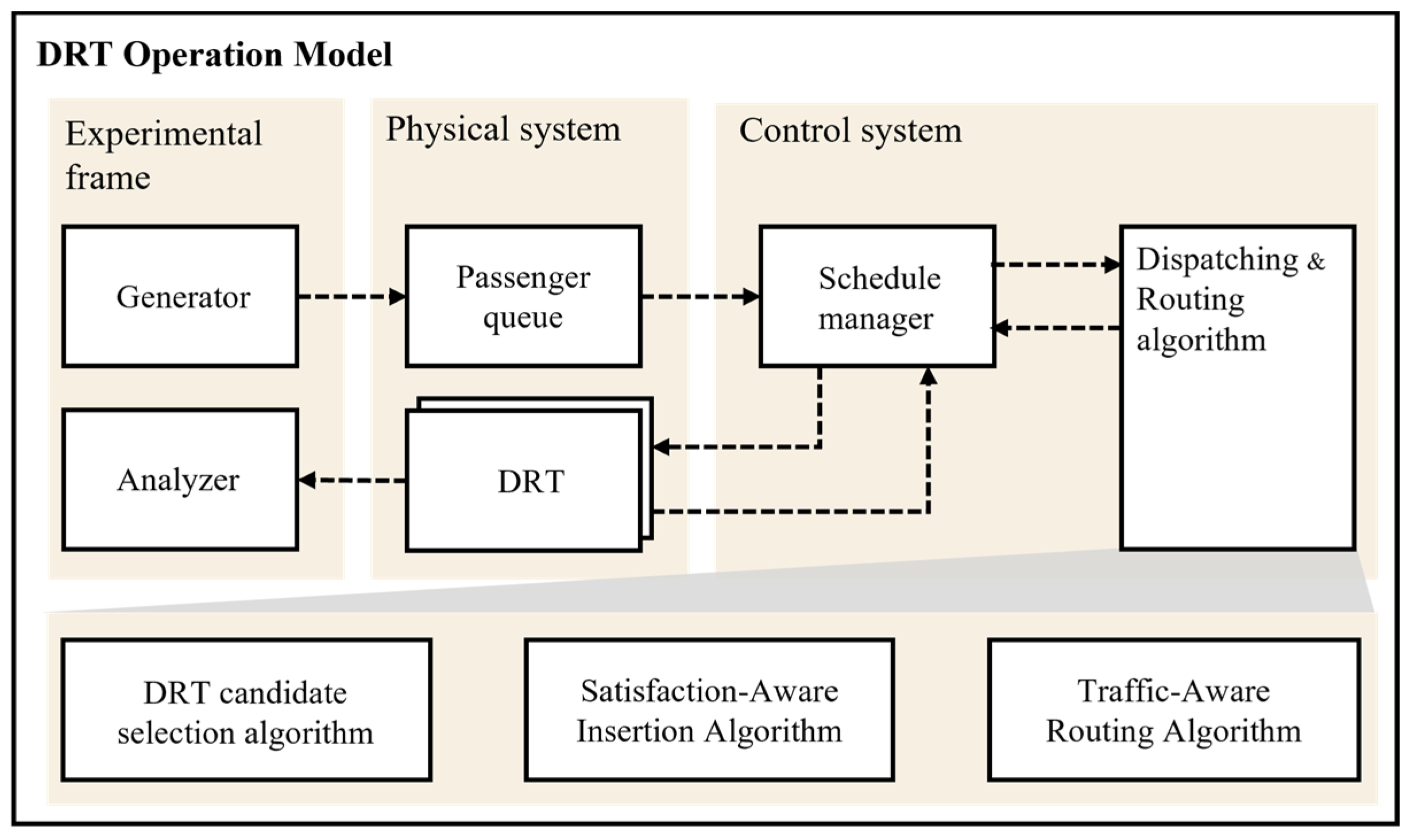
The simulation model is then designed and implemented using the DEVS formalism. The model consists of three main components: (i) a Physical System representing entities with explicit state changes, such as passengers and DRT vehicles; (ii) a Control System responsible for assigning and managing passenger and vehicle schedules; and (iii) an Experimental Frame that governs overall simulation execution, including passenger generation and performance analysis. Dynamic nodes are introduced to allow passenger requests to originate at locations beyond predefined network nodes, thereby improving spatial realism.

For dispatching and routing decisions, three core algorithms are developed: a Fréchet distance-based candidate vehicle selection algorithm, a satisfaction-aware final vehicle assignment algorithm, and a congestion-aware path planning algorithm. Together, these algorithms support efficient and realistic DRT operations under dynamic demand and traffic conditions.

2.2. Simulation Model Development

Simulation Modeling

In this stage, a simulation model is designed and implemented to represent DRT operations. The model adopts the DEVS formalism to define a modular and hierarchical structure that clearly specifies the relationships and state transitions among model components. This structure enables comparative experiments across different algorithms, and in this study, multiple algorithms are applied to reflect realistic operational scenarios [31,32].

Figure 4 illustrates the overall simulation model structure for DRT operations. The model consists of three primary components: the Experimental Frame, the Physical System, and the Control System. The Experimental Frame includes a Generator model, which produces passenger requests by specifying request times and pickup and drop-off locations based on estimated DRT demand, and an Analyzer model, which conducts comprehensive performance analysis after each experiment and across repeated simulation runs. The Physical System represents actual passengers and DRT vehicles. Each DRT vehicle is modeled individually and moves along its assigned route based on the schedule provided by the Schedule Manager model, continuously updating its current location. The Passenger Queue model represents the full process by which generated passengers issue service requests, board assigned vehicles, and ultimately alight at their destinations. In the proposed model, passenger requests are processed according to a first-come-first-served (FCFS) rule. When a passenger request is generated, it is stored in the Schedule Manager in the order of arrival and forwarded to the scheduling process in the same order.

The Control System manages vehicle schedules in response to passenger requests. It includes a Schedule Manager model, which handles schedule generation and sequencing, and a Dispatching & Routing Algorithm model, which performs vehicle assignment and route generation. The integration of the candidate vehicle selection algorithm, the satisfaction-aware passenger insertion algorithm, and the congestion-aware path planning algorithm is intended to reduce computational complexity while enabling a realistic simulation environment.

In addition, the simulation model allows passengers to request service from arbitrary locations rather than predefined stops, similar to real taxi operations, thereby enhancing model flexibility. This is implemented through dynamic nodes, which enable the reproduction of more complex and diverse traffic situations.

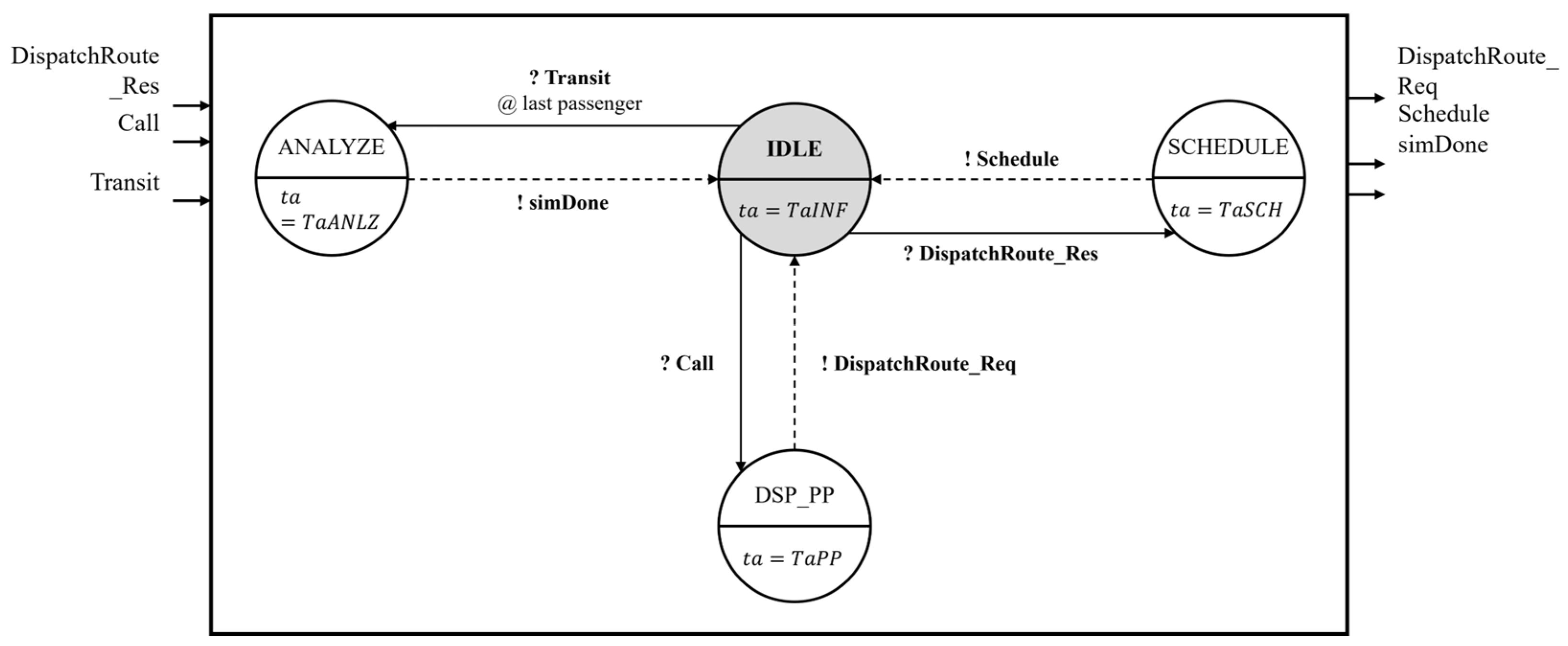
The Schedule Manager is a core control model responsible for generating and managing vehicle schedules based on passenger request information and the real-time positions of DRT vehicles. As illustrated in Figure 5, the model operates through a sequence of state transitions that govern the scheduling process from the arrival of a passenger request to the completion of vehicle operations.

At the beginning of the simulation, the Schedule Manager remains in an IDLE state while waiting for external events. Upon receiving a new passenger request message from the Passenger Queue, it transitions to a processing state (DSP_PP) to initiate vehicle assignment and route planning. In this stage, the DspPpManager performs feasibility evaluation for the incoming request by checking vehicle capacity, route insertion feasibility, and potential service delays. If no feasible vehicle assignment can be identified, the request is rejected and represented as a dispatch failure within the scheduling process. In this state, the Schedule Manager sends a request to the Dispatching & Routing Manager to generate candidate vehicle assignments and routes.

Once a candidate schedule is received from the Dispatching & Routing Manager, the Schedule Manager moves to the SCHEDULE state, where the finalized scheduling information is delivered to the corresponding DRT vehicle model for execution. After the vehicle completes its operation and reports that the last passenger has been dropped off, the Schedule Manager transitions to the ANALYZE state to finalize and manage the scheduling outcome.

These state transitions are event-driven and executed instantaneously, enabling the Schedule Manager to systematically coordinate vehicle assignment and scheduling within the DRT system.

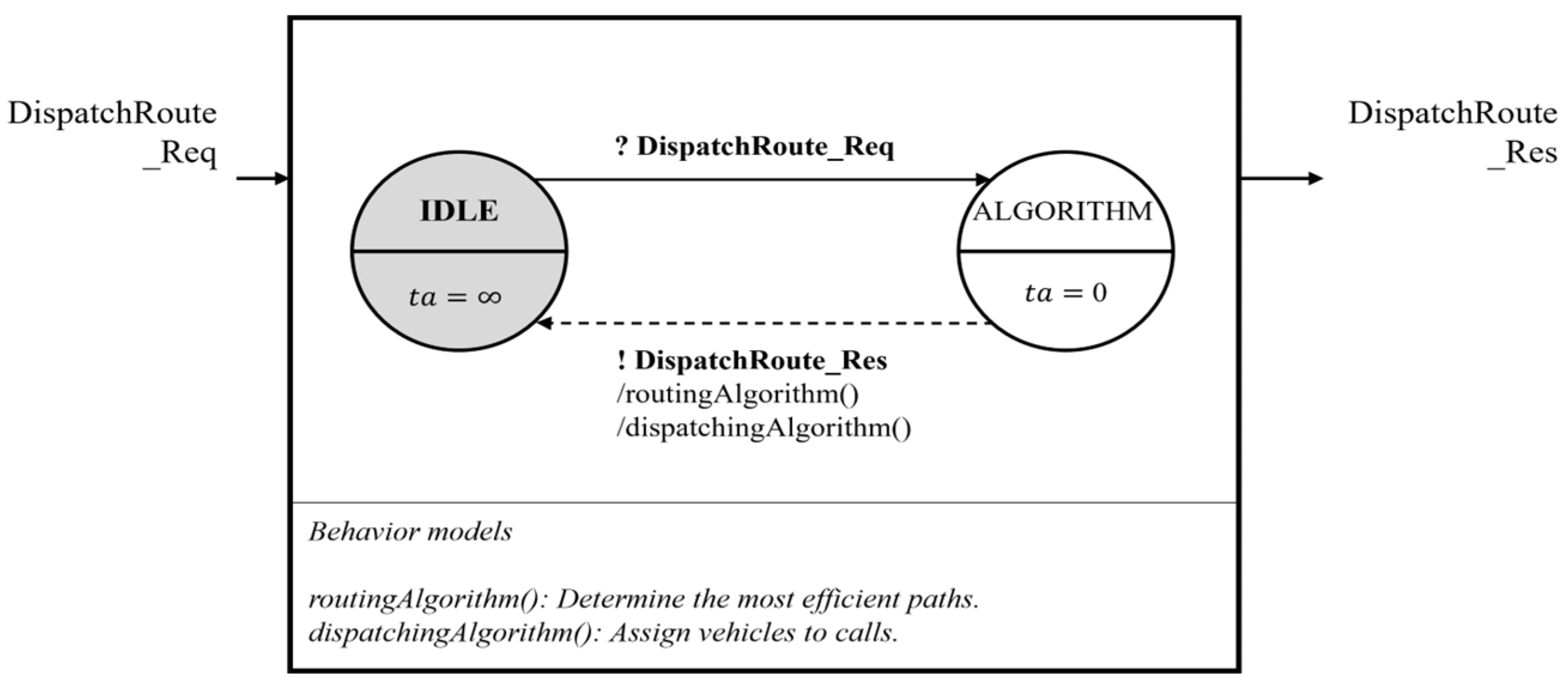
Figure 6 shows the structure of the Dispatching & Routing atomic model. When the Schedule Manager requests vehicle assignment and route planning, this atomic model is activated. During this process, the configured algorithms are executed to identify and assign the optimal vehicle, and the resulting schedule is transmitted back to the Schedule Manager model.

The model is designed and implemented in a modular manner based on the DEVS formalism, allowing each atomic component to operate independently as long as its input and output interfaces remain consistent. As a result, the Dispatching & Routing atomic model can encapsulate and modify vehicle assignment and routing algorithms while preserving its interface functions. This modularity enables flexible application of different algorithms and facilitates optimization of overall model performance [33,34].

2.3. Proposed Algorithms

2.3.1. Fréchet Distance-Based Candidate Vehicle Selection

Fréchet distance is a similarity measure between two curves that considers the geometric structure and the ordering of points along the paths. Formally, the Fréchet distance between two routes is defined as the minimum value of the maximum distance between corresponding points along the two curves while traversing them. This property allows the metric to capture not only the spatial proximity between routes but also the overall route shape and traversal order.

In this study, the Fréchet distance is used to evaluate the similarity between an existing vehicle route and a candidate route generated by inserting a new passenger request. To further improve route comparison, vector directionality is incorporated so that both the spatial distance and the directional characteristics of routes are considered during similarity evaluation.

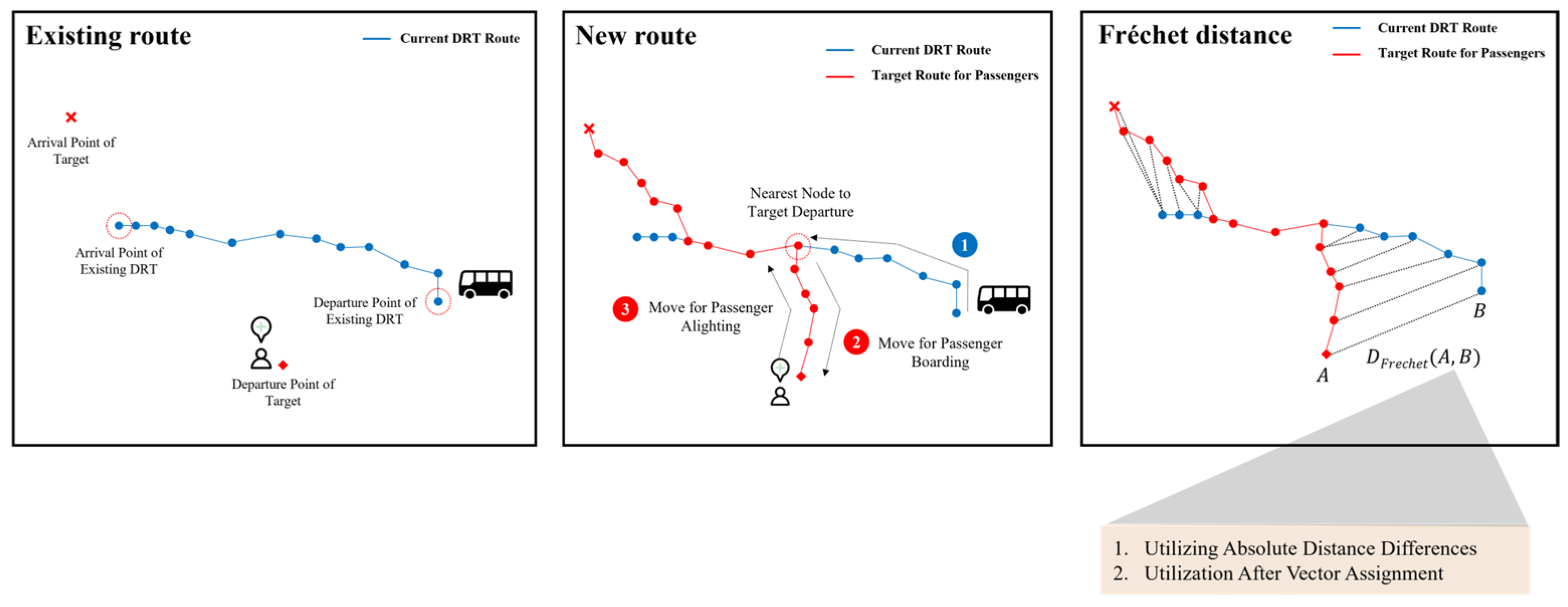
Figure 7 illustrates the conceptual process of the proposed Fréchet Distance-Based Candidate Vehicle Selection (FD-CVS) algorithm. Initially, as shown in the first panel, a DRT vehicle follows a predefined route (represented by blue nodes and links) that serves existing passenger requests. When a new passenger request occurs (marked by the red diamond and cross), the system must evaluate how effectively this request can be accommodated within the vehicle’s current route.

In the second panel, a candidate route is generated by inserting the new passenger’s pickup and drop-off locations into the existing route. This process involves identifying the closest node on the vehicle’s current route to the passenger’s origin (1), adding a path to serve the pickup location (2), and then appending a route segment to the passenger’s destination (3). The resulting combined route, highlighted in red, represents the potential adjustment needed to accommodate the new request. The third panel shows the calculation of similarity between the existing and the adjusted routes using the Fréchet distance. This metric quantifies the directional similarity between the original (blue) and modified (red) routes. A smaller Fréchet distance indicates less deviation from the current route. The FD-CVS algorithm computes this distance for all feasible vehicles and selects the top three vehicles with the smallest Fréchet distances. This selection substantially reduces the computational burden of subsequent vehicle assignment and routing processes. The detailed procedure of the FD-CVS algorithm is provided in Algorithm 1. The FD-CVS algorithm consists of three main stages. In the first stage, the algorithm determines whether the passenger’s request point corresponds to an existing network node or a dynamic node. If the request originates from a dynamic node, the expected travel time is calculated using the calculateTimeToNode function. If the request point already exists within the fixed network, the arrival time is also computed using the calculateTimeToNode function. This initial step identifies the feasibility of each vehicle for serving the new request. Compared with simple distance-based metrics such as Euclidean distance or path overlap measures, the Fréchet distance captures the overall route geometry and traversal order, making it particularly suitable for evaluating route similarity in DRT vehicle assignment problems.

Algorithm 1. Frechet Distance-based Candidate Vehicle Selection (FD-CVS)

1.   FUNCTION selectCandidateVehiclesByFrechetDistance(newPassengerRequest, availableVehicles, shortestPaths, networkInfo) 2. 3.    INITIALIZE vehicleSimilarityScores as empty list 4.    SET timeLimit as predefined maximum allowed waiting time 5. 6.    FOR (vehicleID, vehicle) IN availableVehicles DO 7. 8.       IF isDynamicNode(newPassengerRequest.departureNode) THEN 9.         timeToDeparture ← calculateTimeToDynamicNode(vehicle, newPassengerRequest, shortestPaths) 10.     ELSE 11.       timeToDeparture ← calculateTimeToNode(vehicle, newPassengerRequest.departureNode, shortestPaths) 12. 13.     IF timeToDeparture ≤ timeLimit THEN 14.       passengerRoute, passengerRouteVector ← calculatePassengerRoute(newPassengerRequest, closestNode, networkInfo) 15.       vehicleRouteVector ← calculateVehicleRouteVector(vehicle.currentPath, networkInfo) 16.       similarityScore ← computeFrechetDistance(vehicleRouteVector, passengerRouteVector) 17. 18.       APPEND (vehicleID, similarityScore) TO vehicleSimilarityScores 19.     ENDIF 20. 21.   ENDFOR 22. 23.   topCandidateVehicles ← SORT vehicleSimilarityScores by similarityScore ascending and SELECT top 3 vehicles 24.   filteredVehicles ← FILTER availableVehicles BY topCandidateVehicles 25. 26.   RETURN filteredVehicles

In the second stage, the Fréchet distance is computed only for vehicles that satisfy the feasibility criterion. The computation uses the computeFréchetDistance function, formally described in Algorithm 2, to evaluate the directional similarity between each vehicle’s existing route and the corresponding adjusted route. In the final stage, candidate vehicles are selected based on their computed Fréchet distances. Vehicles are sorted in ascending order of their similarity scores, and the top three are selected as final candidates. This selective process effectively limits computational overhead and enhances the real-time responsiveness of DRT system operations. Algorithm 2 outlines the Fréchet distance calculation using dynamic programming with memoization. Given two routes represented as ordered route sequences, P = (P[0], …, P[n]) and Q = (Q[0], …, Q[m]), where each element denotes a node (or route point) on the path, the algorithm recursively computes the Fréchet distance while storing previously calculated values to avoid redundant computation. Here, n and m denote the last indices of routes P and Q, respectively, and i and j are intermediate index variables representing the current node (or point) positions being compared in the two routes.

Algorithm 2. Frechet Distance Calculation using Dynamic Programming (FD-DP)

1.   FUNCTION computeFrechetDistance(curveP, curveQ): 2. 3.    numPointsP: = LENGTH(curveP) 4.    numPointsQ: = LENGTH(curveQ) 5. 6.    //Memoization array initialization 7.    frechetMemo: = ARRAY[numPointsP][numPointsQ] INITIALIZED TO −1 8. 9.    //Recursive function to compute Frechet distance 10.  FUNCTION calculateDistanceRecursive(i, j): 11. 12.    //Return memoized result if available 13.    IF frechetMemo[i][j] > −1 THEN 14.      RETURN frechetMemo[i][j] 15.    END IF 16. 17.    //Base case: first point in both curves 18.    IF i = 0 AND j = 0 THEN 19.      frechetMemo[i][j]: = Distance(curveP[0], curveQ[0]) 20. 21.    //If only one point in curveQ 22.    ELSE IF i > 0 AND j = 0 THEN 23.      frechetMemo[i][j]: = MAX( 24.        calculateDistanceRecursive(i − 1, 0), 25.        Distance(curveP[i], curveQ[0]) 26.      ) 27.     28.    //If only one point in curveP 29.    ELSE IF i = 0 AND j > 0 THEN 30.      frechetMemo[i][j]: = MAX( 31.        calculateDistanceRecursive(0, j − 1), 32.        Distance(curveP[0], curveQ[j]) 33.      ) 34 35.    //General case 36.    ELSE 37.      minPrev: = MIN( 38.        calculateDistanceRecursive(i − 1, j), 39.        calculateDistanceRecursive(i − 1, j − 1), 40.        calculateDistanceRecursive(i, j − 1) 41.      ) 42.      frechetMemo[i][j]: = MAX(minPrev, Distance(curveP[i], curveQ[j])) 43.    END IF 44. 45.    RETURN frechetMemo[i][j] 46.  END FUNCTION 47. 48.  //Call recursive function to get Frechet distance 49.  RETURN calculateDistanceRecursive(numPointsP − 1, numPointsQ − 1) 50. 51. END FUNCTION

Three cases are considered, using a dynamic programming formulation to obtain the Fréchet distance between the two routes from the final entry c(n, m) of the memoization matrix, as follows:

1.

Base case (starting point of both routes):

c(0, 0) = distance P[0], Q [0]

(1)

2.

Single-point base case (one route at the starting point):

c(i, 0) = max{c(i − 1, 0), distance P[i], Q[0]}

(2)

c(0, j) = max{c(0, j − 1), distance P[0], Q[j]}

(3)

3.

General recursive case:

c(i, j) = max{min{c(i − 1, j), c(i, j − 1), c(i − 1, j − 1), distance P[i], Q[j]}}

(4)

By accurately quantifying route similarity, the proposed method improves computational efficiency during candidate vehicle selection.

2.3.2. Congestion-Aware Path Planning

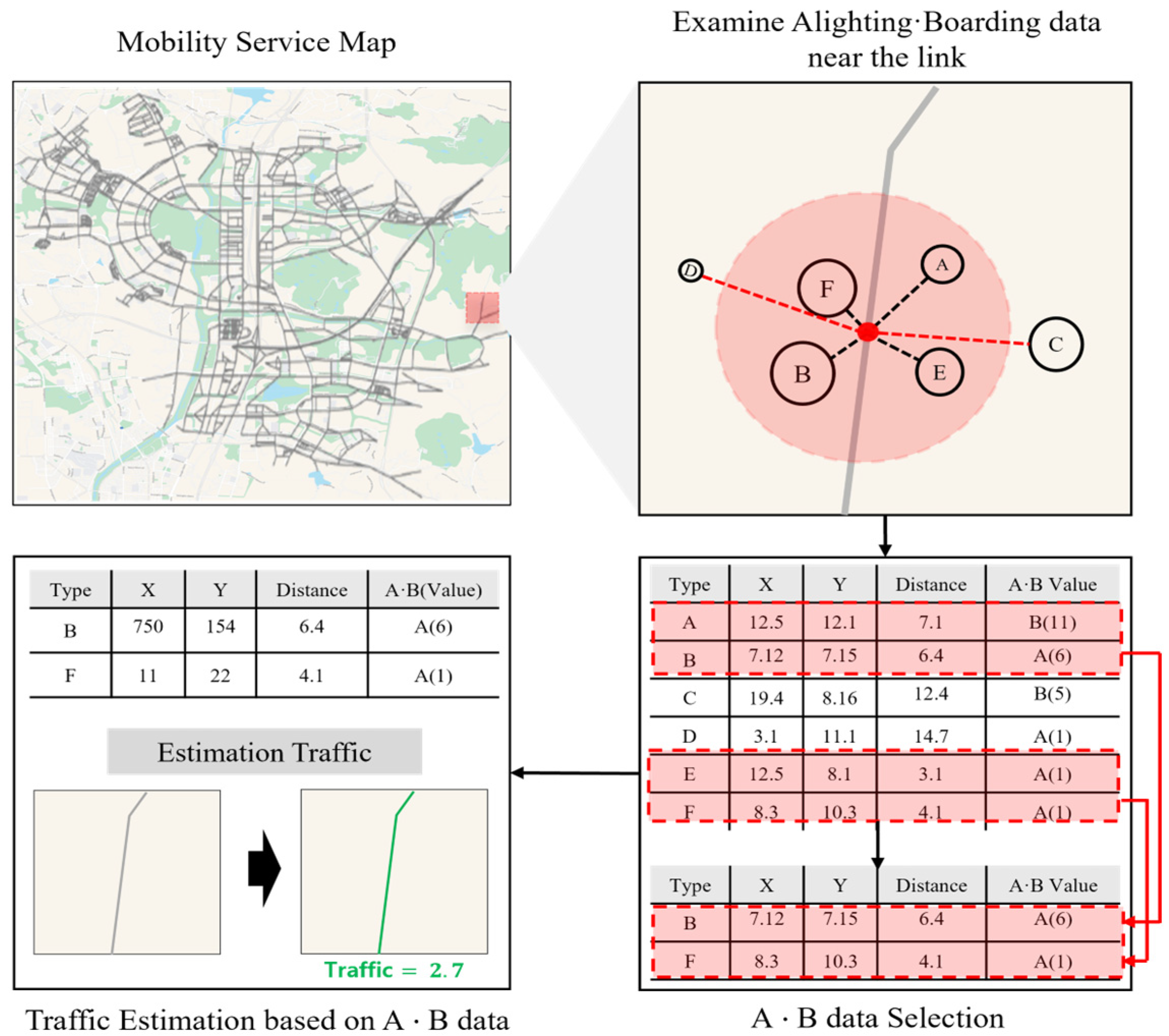
Figure 8 summarizes the conceptual structure of the proposed Congestion-Aware Path Planning (CA-PP) algorithm, which consists of four stages. In the first stage, target road segments (links) for route planning are identified. Specifically, all road segments within the potential paths from a vehicle’s current location to the passenger’s pickup or destination node are selected.

In the second stage, the algorithm estimates traffic volumes on each selected road segment, which is a core feature of the CA-PP method. While previous studies estimate traffic conditions using detailed traffic flow models or learning-based prediction approaches [16,35], the present study adopts a simplified link-level approximation of traffic volume to maintain computational efficiency within the DRT simulation framework. This estimation considers both the number of passengers boarding and alighting at nearby nodes (stations) and their distances to the corresponding road segment. The process is defined mathematically in Equation (5), which calculates the estimated traffic volume L_i for link A − B as

$$Estimated Traffic Link(L_i)=\sum _{i=1}^n{V}_{i,A-B}\times {\displaystyle \frac{C_r-d_{i, A-B}}{C_r}}$$

(5)

Here, C_r denotes the radius around the link used to identify nearby traffic activity, V_i,A−B represents the number of passengers boarding or alighting at the i-th station within that radius around link AB, and d_i,A−B is the distance from the i-th station to the midpoint of link A − B. The estimated traffic volumes are then classified into three congestion categories: “Free-flow” for values of 2.36 or lower, “Moderate” for values between 2.36 and 14.51, and “Congested” for values exceeding 14.51. In this study, the estimated traffic volume is used as an abstracted link-level indicator of surrounding traffic conditions rather than a direct physical traffic-flow measurement. Therefore, the model does not explicitly account for link capacity, road width, or detailed microscopic interactions among mixed traffic flows.

In the third stage, each road segment is explicitly assigned a congestion level based on the estimated traffic volume. Travel times are adjusted accordingly. Under “Free-flow” conditions, the original travel time is used without modification. Under “Moderate” conditions, travel time is multiplied by 1.5, and under “Congested” conditions, it is doubled. This adjustment allows the route planning process to realistically reflect traffic conditions. In the fourth stage, congestion levels are visually mapped and clearly represented, enabling explicit integration of real-traffic information during route selection.

Subsequently, the proposed path planning algorithm (Algorithm 3) uses the congestion data to determine the optimal path from a departure node to a destination node. The algorithm extends the conventional A* method by explicitly incorporating road congestion, thereby improving the realism and practicality of the generated routes.

Algorithm 3. Congestion-Aware Path Planning (CA-PP) algorithm

1.   FUNCTION congestionAwareRouting(X_start, X_end) 2.    OPEN_list ← {X_start}, where f(X_start)=heuristicDistance(X_start, X_end), g(X_start)=0 3.    CLOSE_list ← {} 4. 5.    WHILE OPEN_list is not empty DO 6.     X_n ← node in OPEN_list with lowest f(X) 7.     remove X_n from OPEN_list 8.     add X_n to CLOSE_list 9. 10.   IF X_n = X_end THEN BREAK 11. 12.   FOR each adjacent node X_i of X_n DO 13.     IF X_i ∈ CLOSE_list THEN CONTINUE 14. 15.     tentative_g ← g(X_n) + edgeDistance(X_n, X_i) 16. 17.     IF X_i ∉ OPEN_list THEN 18.      X_i.parent ← X_n 19.      g(X_i) ← tentative_g 20.      h(X_i) ← heuristicDistance(X_i, X_end) 21.      IF TrafficCongestionLevel(X_i) ≥ 10 THEN 22.        adjustedCost(X_i) ← 2 × g(X_i) 23.      ELSE IF TrafficCongestionLevel(X_i) ≥ 5 THEN 24.        adjustedCost(X_i) ← 1.5 × g(X_i) 25.      ELSE 26.        adjustedCost(X_i) ← g(X_i) 27.      END IF 28.      f(X_i) ← g(X_i) + h(X_i) + adjustedCost(X_i) 29.      add X_i to OPEN_list 30.     ELSE 31.      IF tentative_g + heuristicDistance(X_i, X_end) + adjustedCost(X_i) < f(X_i) THEN 32.        X_i.parent ← X_n 33.        g(X_i) ← tentative_g 34.        f(X_i) ← g(X_i) + heuristicDistance(X_i, X_end) + adjustedCost(X_i) 35.      END IF 36.     END IF 37.   END FOR 38. 39.   Resort OPEN_list by f(X) values 40.  END WHILE 41. 42.  X_p ← X_end 43.  Path_list ← {X_p} 44.  WHILE X_p ≠ X_start DO 45.    X_p ← X_p.parent 46.    insert X_p at beginning of Path_list 47.  END WHILE 48.   49.  RETURN Path_list 50. END FUNCTION

The algorithm takes as input the start node (X_start) and the end node (X_end) It employs two lists—the OPEN and CLOSE lists—to manage candidate nodes for exploration. Nodes are evaluated using the combined cost function:

f (X) = g(X) + h(X) + t(X),

(6)

where g(X) is the accumulated travel cost from departure to current node, h(X) is the heuristic Euclidean distance from the current node to the destination, and t(X) is an additional cost component reflecting road congestion.

Specifically, t(X) is dynamically adjusted based on congestion level. If the traffic value exceeds 14.51 (Congested), the travel cost is doubled. If it lies between 2.36 and 14.51 (Moderate), the cost is multiplied by 1.5. If it is 2.36 or below (Free-flow), no additional adjustment is applied. During node expansion, the node with the lowest combined evaluation score is prioritized, ensuring selection of a route that realistically reflects traffic conditions. Importantly, the CA-PP algorithm is not applied to all vehicles. It is executed only for the top three candidate vehicles previously identified by the FD-CVS algorithm. By restricting execution to this reduced candidate set, the computational efficiency and responsiveness of the DRT system are substantially improved. This simplified congestion representation was adopted to reduce computational complexity and support real-time path planning in the DRT system. Accordingly, the CA-PP algorithm should be interpreted as a link-level approximation of traffic conditions rather than a full traffic-flow model with explicit capacity constraints.

2.3.3. Satisfaction-Aware Vehicle Assignment

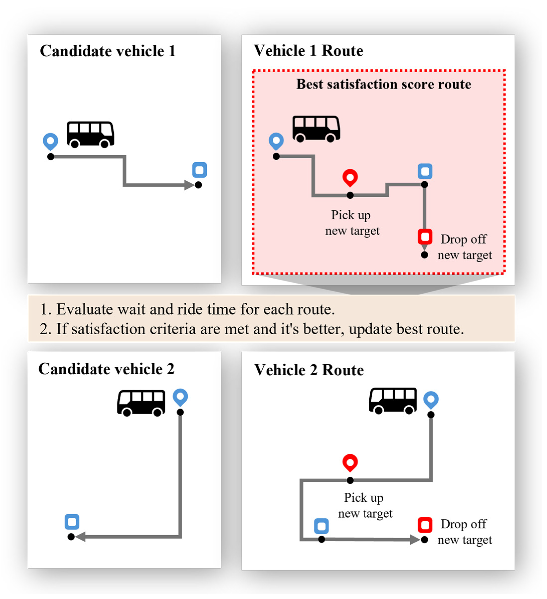
Figure 9 illustrates the concept of the Satisfaction-Aware Vehicle Assignment (SA-VA) algorithm. The figure shows two candidate vehicles identified through the Fréchet distance-based selection and the congestion-aware path planning stages, along with example routes generated for each vehicle. For each candidate vehicle, a route incorporating the new passenger’s pickup and drop-off locations is constructed. The passenger’s waiting time and in-vehicle travel time are then calculated for each route. These two metrics serve as the primary components of the satisfaction score, and all candidate routes are evaluated using the same criteria. The SA-VA algorithm computes satisfaction scores for all candidate routes and selects the route with the highest score as the final solution. If a newly evaluated route satisfies the satisfaction criteria and outperforms the currently selected route, the optimal solution is updated. Thus, the algorithm does not terminate after a single evaluation but sequentially compares candidate routes and continuously updates the best solution.

The proposed Satisfaction-Aware Vehicle Assignment (SA-VA) algorithm (Algorithm 4) determines the final vehicle and route for serving a new passenger based on the candidate routes generated in the previous stages. The algorithm takes as input the existing vehicle route (existingRoute), passenger count changes at each stop (psgrCountChange), the new passenger’s pickup and drop-off locations (targetDeparture, targetArrival), the number of new passengers (targetPsgrNum), the current onboard passenger count (curPsgrNum), and the maximum vehicle capacity (shuttleMax).

Algorithm 4. Satisfaction Aware Vehicle Assignment

1.   FUNCTION SatisfactionAwareOptiamlPassengerInsertion (existingRoute, psgrCountChange, targetDeparture, targetArrival, targetPsgrNum, curPsgrNum, shuttleMax) 2. 3.    bestRoute := None 4.    bestTotalTime := Infinity 5.   6.    FOR EACH (i, j) IN all_positions DO 7.      candidateRoute := existingRoute[0:i] + [targetDeparture] + existingRoute[i:j] + [targetArrival] + existingRoute[j:end] 8.      candidatePsgrChange := psgrCountChange[0:i] + [+targetPsgrNum] + psgrCountChange[i:j] + [-targetPsgrNum] + psgrCountChange[j:end] 9. 10.    possiblePsgrNum := curPsgrNum 11.    overCapacity := FALSE 12. 13.    FOR k FROM 0 TO length(candidatePsgrChange) - 1 DO 14.      possiblePsgrNum := possiblePsgrNum + candidatePsgrChange[k] 15.      IF possiblePsgrNum > shuttleMax THEN 16.        overCapacity := TRUE 17.        BREAK 18.      END IF 19.    END FOR 20. 21.    IF overCapacity THEN 22.      CONTINUE 23.    END IF 24. 25.    totalTime := calculateShortestPath(candidateRoute) 26.    passengerWaitingOK := evaluateWaitingTime(candidateRoute) 27.    passengerTravelIncreaseOK := evaluatePassengerTravelIncrease(candidateRoute) 28. 29.    IF passengerWaitingOK AND passengerTravelIncreaseOK THEN 30.      IF totalTime < bestTotalTime THEN 31.        bestTotalTime := totalTime 32.        bestRoute := candidateRoute 33.      END IF 34.    END IF 35.  END FOR 36. 37.  RETURN best_point 38. END FUNCTION

Candidate routes (candidateRoute) are generated by inserting the new passenger’s pickup and drop-off nodes into all feasible positions along the existing route. For each candidate route, the algorithm evaluates the cumulative number of passengers onboard (possiblePsgrNum) throughout route execution to ensure that the vehicle capacity constraint (shuttleMax) is not violated at any point. Routes that exceed the maximum capacity are excluded from further consideration, ensuring realistic operational feasibility.

For the remaining feasible routes, the algorithm computes the total travel time (totalTime) and evaluates passenger satisfaction. Specifically, satisfaction is assessed using the new passenger’s waiting time and the increase in in-vehicle travel time, calculated via the functions evaluateWaitingTime() and evaluatePassengerTravelIncrease(), respectively. The increase in in-vehicle travel time is measured relative to the passenger’s previously expected arrival time under the current route before inserting the new passenger request. This measure represents the additional delay experienced by passengers already on board when the vehicle route is modified to accommodate the new request.

Finally, among all candidate routes that satisfy the passenger satisfaction constraints, the algorithm selects the route with the minimum total travel time as the optimal solution. Through this process, the proposed method achieves an optimal vehicle assignment by prioritizing passenger satisfaction while maintaining operational efficiency.

3. Experiments

This section presents the experiments conducted to validate the proposed simulation framework and algorithms. The experimental study is organized into two main stages. In the first stage, data modeling validation and simulation model validation are performed to verify whether the framework operates as intended. In the second stage, the satisfaction-aware final vehicle selection algorithm and the Fréchet distance-based candidate vehicle selection algorithm are applied to evaluate their performance and computational efficiency.

3.1. Experimental Design

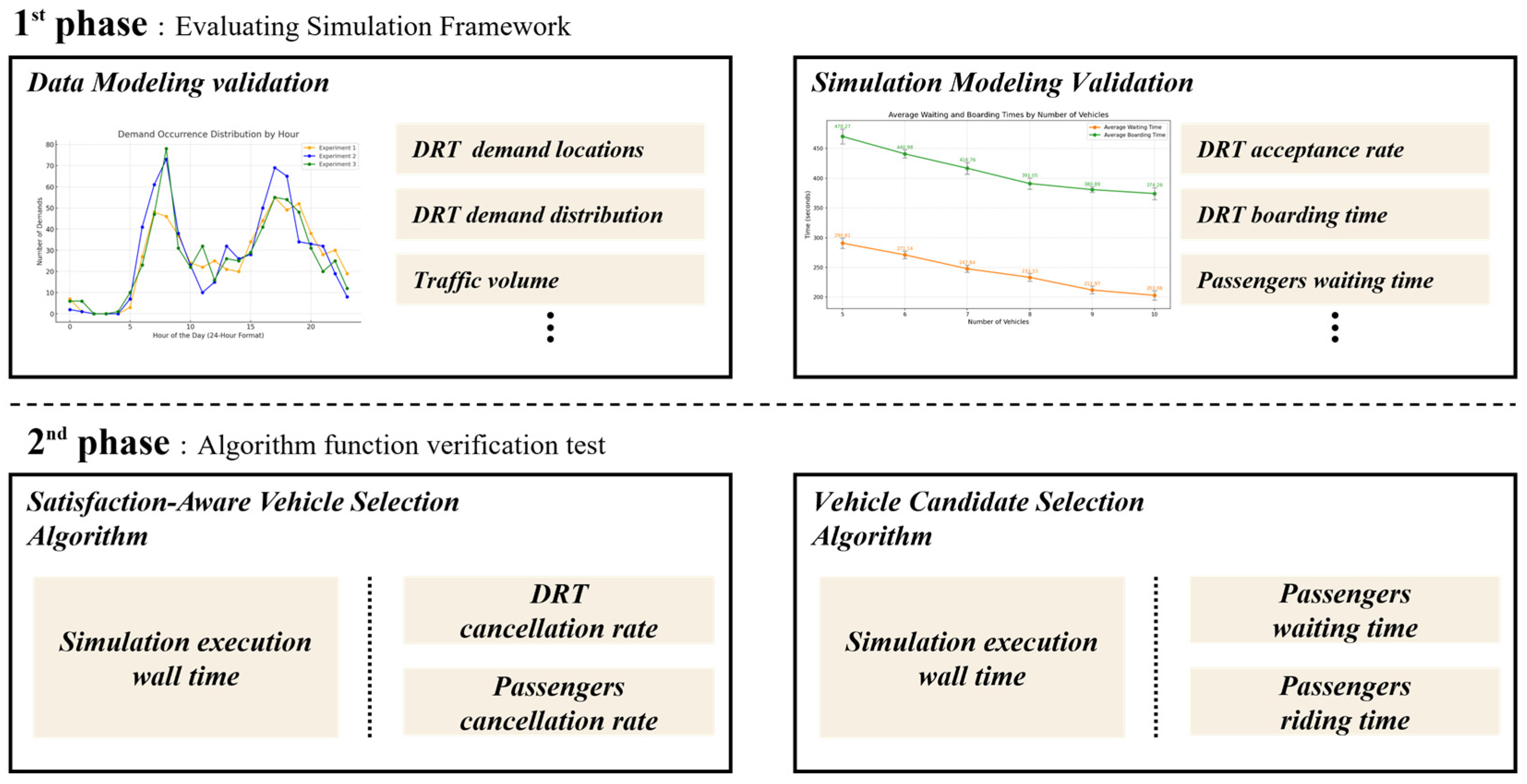
The simulation framework (Figure 10) adopts a two-stage experimental structure. The first stage focuses on verifying the correctness and stability of the designed and implemented simulation framework. This stage consists of data modeling validation and simulation model validation.

In the data modeling validation phase, real-world public transportation data, including passenger demand and traffic volume information, are incorporated to assess whether the model adequately reflects realistic operating conditions. The simulation model validation phase analyzes key performance indicators of the DRT system, such as average passenger waiting time and riding time, to confirm whether the model behaves as expected. In addition, the effect of varying fleet sizes on system performance and operational stability is examined.

The second stage evaluates whether the proposed algorithms function as intended within the simulation environment. Specifically, the satisfaction-aware final vehicle selection algorithm and the Fréchet distance-based candidate vehicle selection algorithm are assessed. The satisfaction-aware algorithm is designed to reduce passenger waiting time and improve overall service satisfaction. Accordingly, vehicle cancellation rate and passenger cancellation rate are used as the primary evaluation metrics.

To indirectly assess computational complexity, simulation execution times with and without the proposed algorithms are compared. In addition, relative performance differences under identical execution times are examined. The Fréchet distance-based candidate vehicle selection algorithm is primarily designed to reduce absolute simulation execution time. Therefore, execution time differences with and without this algorithm are used as the main comparison metric. Under equivalent service performance conditions, passenger waiting time and riding time are jointly analyzed to evaluate the impact of candidate vehicle filtering on overall simulation efficiency.

3.2. Simulation Parameters

Table 2. Uncontrollable simulation parameters.

Parameter Name	Parameter Level	Parameter Description
City	Dongtan 1 & 2 New Cities	Subject of the simulation
City area	34.04 km2 (combined area)	Total area of the target city
Map node	1088 nodes	Number of nodes in the road network
Map link	3136 links	Number of links in the road network
Passenger boarding time	5 s	Time required for a passenger to board the shuttle
Shuttle speed	Maximum road speed + 5 km/h	Maximum allowable speed of the shuttle
Shuttle capacity	9 passengers	Maximum number of passengers per shuttle

describes the target study area used in the simulation experiments. The experimental area corresponds to Dongtan New Towns 1 and 2, covering a total area of approximately 34.04 km². The road network consists of 1088 nodes and 3136 links, each containing spatial coordinate information required for simulation execution.

The maximum shuttle capacity is set to nine passengers. Passenger boarding and alighting times are assumed to be five seconds each. Shuttle travel speed is determined based on the maximum speed assigned to each road link and is allowed to vary within a range of ±5 km/h to reflect realistic driving behavior.

The controllable simulation parameters (

Table 3. Controllable simulation parameters.

Parameter Name	Parameter Level	No. Levels	Parameter Description
No. of shuttles	5, 6, …, 10	6	Number of shuttles used in the simulation
Demand rate	5, 10, 15 (%)	3	Demand rate applied in the simulation
Algorithm (candidate selection)	Applied, not applied	2	Use of Fréchet-distance-based candidate vehicle selection
Algorithm (final insertion)	Applied, not applied	2	Use of satisfaction-based final route insertion

) include the number of shuttles, the demand reflection rate, the application of the Fréchet distance-based candidate vehicle selection algorithm, and the application of the satisfaction-aware final vehicle selection algorithm. The number of shuttles ranges from five to ten. The demand reflection rate is set to 5%, 10%, and 15% of total potential demand. Each algorithm is evaluated under two conditions: applied and not applied. For each parameter configuration, 30 Monte Carlo simulation runs are conducted to ensure statistical reliability [36]. The average values of the performance metrics obtained from these repeated simulations are used for comparative analysis.

3.3. Evaluated Key Performance Indicators (KPIs)

To comprehensively evaluate the performance of the proposed DRT system, several KPIs are defined and analyzed. These KPIs capture both passenger-oriented service quality and system-level operational efficiency. In particular, passenger waiting time and riding time represent service quality from the passenger perspective, while the shuttle acceptance rate reflects the efficiency of resource utilization and demand responsiveness. All KPIs are calculated from simulation outputs and averaged over repeated Monte Carlo experiments to ensure statistical reliability [37] (

Table 4. Evaluated KPIs.

KPI	Description
Passenger waiting time	Average time passengers wait before boarding a shuttle
Passenger riding time	Average time passengers spend onboard the shuttle from boarding to destination
Shuttle acceptance rate	Ratio of passengers out of total received requests successfully assigned to a shuttle

).

3.3.1. Passenger Waiting Time

The first performance indicator is average passenger waiting time, defined as the mean duration from when a passenger request is generated until the passenger boards a shuttle. This metric directly reflects the responsiveness of the DRT system and the effectiveness of dispatching and assignment strategies. Passenger waiting time is a critical indicator of perceived service quality, as excessive delays significantly reduce passenger satisfaction and system attractiveness [38,39,40,41]. Let W_m denote the waiting time of passenger m, and let A be the set of all served passengers. The average passenger waiting time is defined as

$$AW={\displaystyle \frac{{\sum }_{m\in A}{W}_m}{\left|A\right|}}$$

(7)

This KPI is used to evaluate how efficiently the system responds to passenger requests under different algorithmic configurations and demand scenarios.

3.3.2. Passenger Riding Time

The second performance indicator is average passenger riding time, which measures the mean duration that passengers spend onboard the shuttle from boarding to arrival at their destination. This metric reflects the efficiency of route construction and the impact of ride sharing on the passenger travel experience.

Passenger riding time is particularly important in DRT systems, where route detours and shared rides may increase in-vehicle travel time compared with direct trips [42,43]. This indicator is therefore used to assess the trade-off between operational efficiency and passenger convenience. Let R_m denote the riding time of passenger m. The average passenger riding time is defined as

$$AR={\displaystyle \frac{{\sum }_{m\in A}{R}_m}{\left|A\right|}}$$

(8)

This KPI enables analysis of how routing strategies, vehicle capacity constraints, and request insertion policies affect passenger travel duration.

3.3.3. Shuttle Acceptance Rate

The third performance indicator is the shuttle acceptance rate, defined as the proportion of passenger requests that are successfully assigned to a shuttle. This metric evaluates the system’s ability to accommodate demand and reflects both fleet adequacy and dispatch effectiveness.

A high acceptance rate indicates that the DRT system can respond effectively to passenger requests without excessive rejections, whereas a low acceptance rate suggests insufficient capacity or inefficient routing decisions. Let N_ac and N_rc denote the number of accepted and rejected requests, respectively. The shuttle acceptance rate is defined as:

$$AAR=100\times {\displaystyle \frac{N_{ac}}{N_{ac}+N_{rc}}}$$

(9)

This KPI is particularly useful for evaluating system robustness under varying demand levels and fleet sizes.

3.3.4. Summary of KPI Evaluation

The KPIs defined in Equations (7)–(9) provide a multidimensional evaluation framework for the DRT system. By jointly considering passenger service quality (waiting and riding times) and operational efficiency (acceptance rate), the framework enables systematic comparison of algorithmic performance across different simulation scenarios.

For each parameter combination, the simulation is executed 30 times using a Monte Carlo approach, and the reported KPI values correspond to the averaged results. This repetition ensures statistical consistency and reliability. In the subsequent analysis, these KPIs are used to comprehensively assess the behavioral characteristics and performance differences in the DRT system under varying algorithmic configurations and demand conditions.

4. Experimental Results

The purpose of this experimental study is to verify and evaluate the performance of the proposed simulation framework and algorithms from multiple perspectives. The results provide a comprehensive analysis of prediction accuracy, boarding efficiency, resource utilization, and algorithmic computational efficiency. Through this analysis, the study assesses how effectively the DRT system can operate under realistic conditions. In particular, data obtained from multiple output variables and repeated experiments enhance the reliability of the evaluation and serve as key criteria for assessing the stability and responsiveness of system operations based on real-time data [44,45].

4.1. Simulation Framework Evaluation

The experiments evaluating the simulation framework were based on public transportation data from Dongtan City and were conducted from two perspectives: validation of data modeling and validation of the simulation model. In the data modeling validation, the number of demand occurrences and the average boarding time for each time period were measured to examine whether demand patterns and traffic volumes were appropriately reflected in the simulation. The results confirm that the public transportation data used in the model exhibit behavior similar to real-world traffic patterns within the simulation environment.

In the simulation model validation, analyses were performed from both passenger and vehicle perspectives. A scenario was introduced in which vehicle operations could be canceled when vehicle satisfaction deteriorated significantly, and the primary reasons for such cancellations were examined. In addition, average waiting times and boarding times were analyzed as the number of vehicles increased in order to verify whether the simulation framework remained stable under conditions of increased vehicle supply. These analyses confirm that the framework functions in accordance with the intended design.

4.2. Data Modeling Evaluation

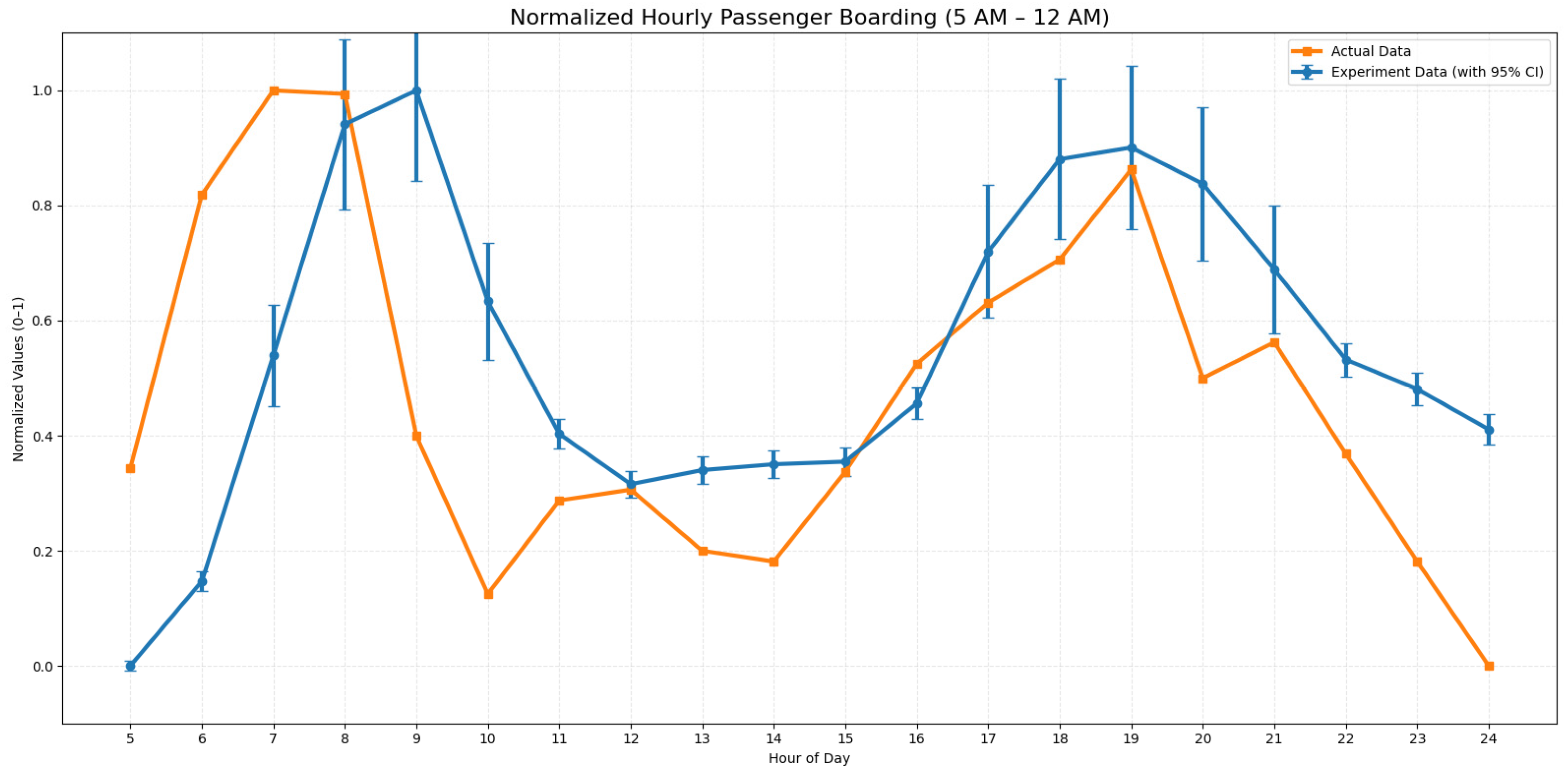
Figure 11 presents the time-of-day distribution of demand generated within the simulation model. The x-axis shows simulation time from 05:00 to 24:00, and the y-axis represents the relative number of passenger occurrences in each period, normalized to the range 0–1 using the minimum and maximum values. The experimental data represent aggregated results from 100 simulation runs, whereas the real-world data correspond to the total number of passengers observed during a single day. Because of the substantial difference in absolute scale, both datasets were normalized to enable meaningful comparison of temporal demand patterns.

The comparison indicates that the simulated time-dependent demand exhibits a pattern similar to actual boarding and alighting trends observed in Dongtan City. This finding suggests that the simulation model effectively captures real-world traffic dynamics and supports the validity of the demand prediction component. In particular, the sharp increases in demand during peak commuting hours—between 06:00 and 08:00 in the morning and between 17:00 and 19:00 in the evening—are consistently reproduced in the simulation, demonstrating the model’s ability to realistically reproduce traffic demand during congested periods. Moreover, the high volume of demand during these periods leads to greater variability, resulting in relatively wider confidence intervals.

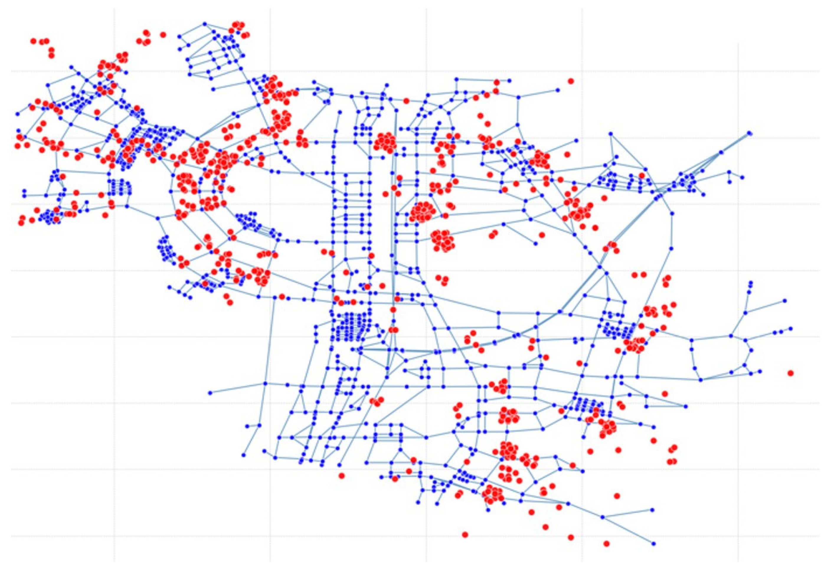
Figure 12 illustrates the spatial distribution of demand generated in the simulation, together with the previously described temporal demand patterns. After confirming that the temporal distribution reflects public transportation usage in Dongtan City, Figure 12 further shows that simulated demand locations tend to coincide with major boarding and alighting points in the real network. This result indicates that the model captures not only temporal but also spatially realistic demand patterns.

As shown in the figure, the simulation adopts a flexible structure in which demand can arise not only at predefined stops but also at locations without fixed nodes through the use of dynamic nodes. These dynamic nodes enable the system to accommodate requests from unpredictable locations, thereby enhancing model adaptability and increasing the practical applicability of the DRT system in real-world settings [46,47,48,49].

4.3. Simulation Model Evaluation

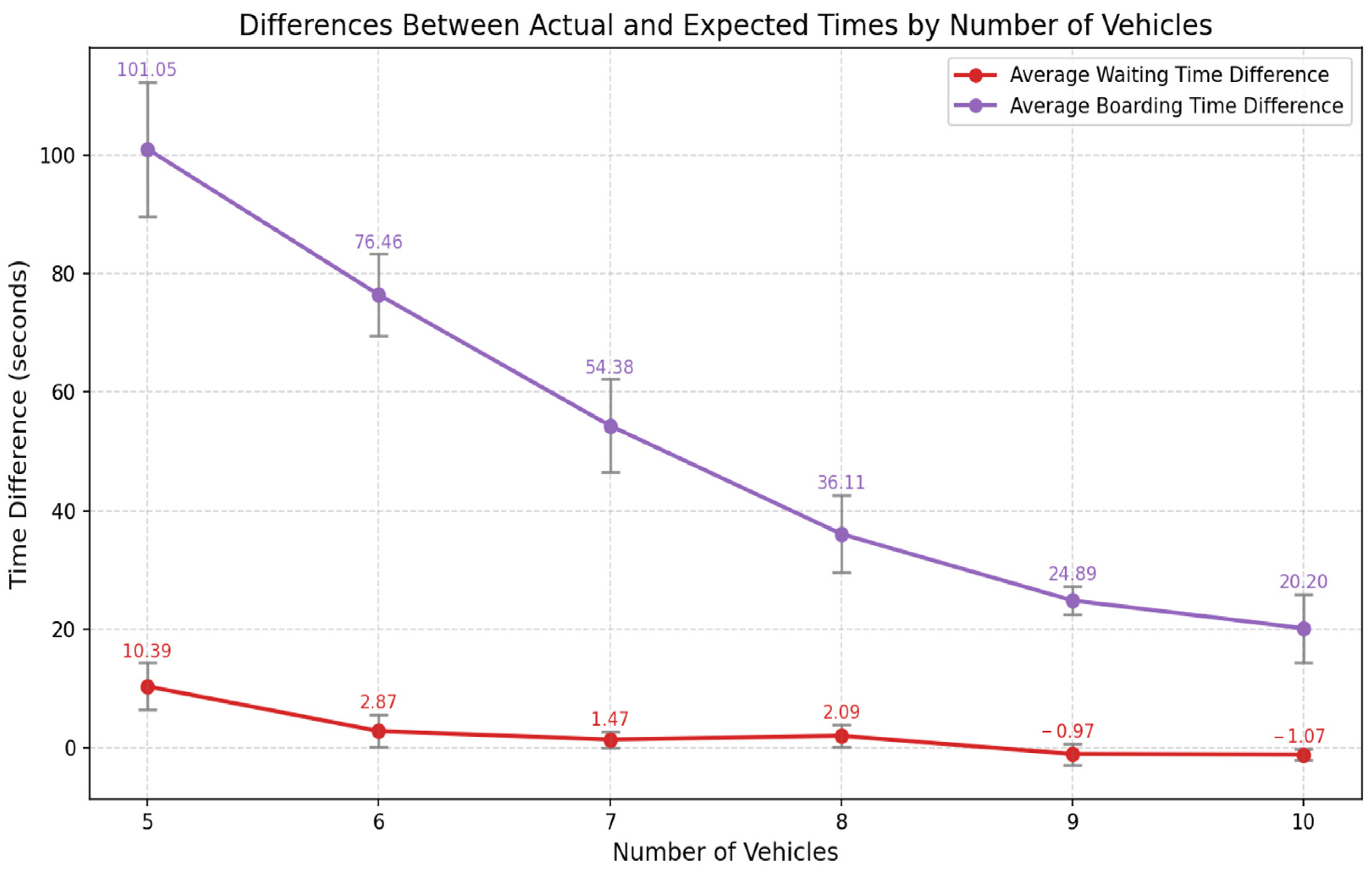
Figure 13 shows that the discrepancy between estimated and actual times decreases as the number of vehicles increases. The x-axis represents the fleet size, and the y-axis indicates the difference between estimated and actual times, measured in seconds. The purple line corresponds to boarding time differences, and the red line represents waiting time differences. Both exhibit a clear downward trend as the fleet size grows.

This result can be attributed to the vehicle assignment strategy, which explicitly considers passenger satisfaction in vehicle selection. Vehicles are chosen to minimize both the increase in waiting time for newly requesting passengers and the increase in boarding time for passengers already onboard. The more rapid reduction in waiting-time discrepancies reflects the higher weight assigned to waiting time in the selection process. This design is based on the assumption that waiting time has a greater impact on passenger satisfaction than in-vehicle boarding time.

4.4. Algorithm Performance Evaluation

The algorithm performance experiments are designed to validate the functionality of the advanced methods incorporated into the simulation framework. In these experiments, both the Fréchet distance-based vehicle candidate selection algorithm and the satisfaction-based final vehicle selection algorithm are evaluated to verify that each operates as intended. The experiments are conducted under three demand reflection rates—5%, 10%, and 15% of total demand. These demand reflection rates were selected to represent different demand levels while maintaining a computationally feasible simulation environment based on the real-world demand extracted from the Dongtan public transportation dataset. In addition, previous transportation simulation studies have also adopted 100 Monte Carlo replications and reported stable comparative performance based on repeated simulation averages [50,51,52]. Following this practice, the present study used 100 Monte Carlo runs to obtain statistically robust comparative results while maintaining reasonable computational cost.

4.4.1. Performance Evaluation of the Fréchet Distance-Based Vehicle Candidate Selection Algorithm

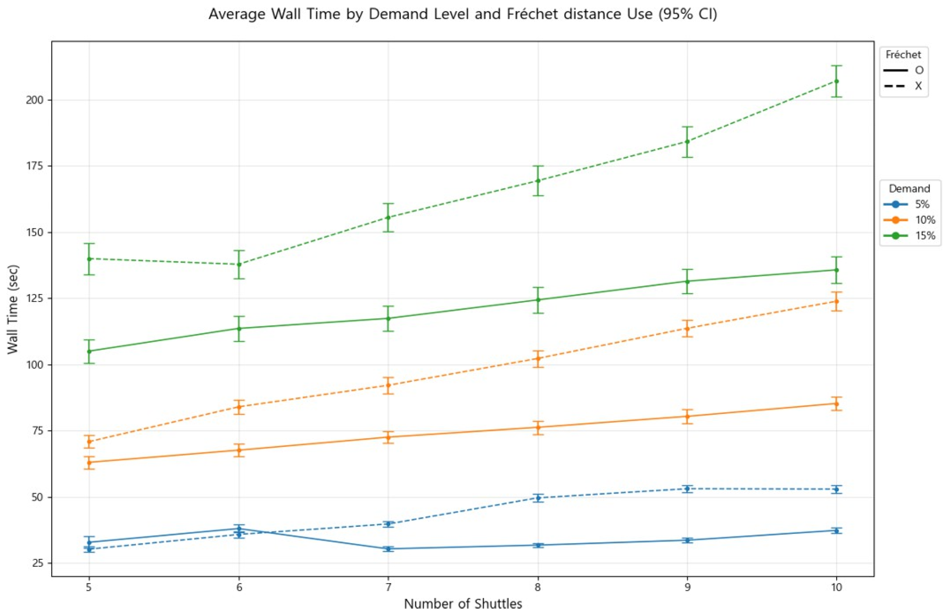
The line styles and colors used in this subsection are defined as follows: solid lines represent cases in which the Fréchet distance-based vehicle candidate selection algorithm is applied, whereas dashed lines indicate cases in which it is not applied. Blue lines correspond to a demand reflection rate of 5%, orange lines to 10%, and green lines to 15%.

Figure 14 illustrates the average wall time for different demand levels as the number of vehicles increases. The x-axis denotes the fleet size, and the y-axis shows the average wall time in seconds. When the demand reflection rate is 15% and the Fréchet distance-based algorithm is not applied, a temporary decrease in average wall time of approximately 2.09 s is observed as the number of vehicles increases from five to six. This behavior can be attributed to an initially insufficient fleet relative to high demand when only five vehicles are available, which increases computational load during dispatching and route planning and compounds service delays. In contrast, under the 5% demand condition with the Fréchet distance-based algorithm applied, the average wall time increases by approximately 2.41 s as the fleet size increases from five to six vehicles. This increase is likely due to the small number of requests under low-demand conditions, which yields a limited set of candidate vehicles. In such cases, the computational overhead associated with Fréchet distance calculations outweighs the benefits of vehicle filtering.

Overall, as the number of vehicles increases, scenarios using the Fréchet distance-based algorithm consistently exhibit shorter wall times than those without it. Specifically, the average wall time is reduced by 9.57 s at 5% demand, 23.59 s at 10% demand, and 44.38 s at 15% demand. These results indicate that, with increasing fleet size and demand, the Fréchet distance-based algorithm effectively reduces the search space and improves computational efficiency. Consequently, the performance benefits become more pronounced as both demand and the number of vehicles grow.

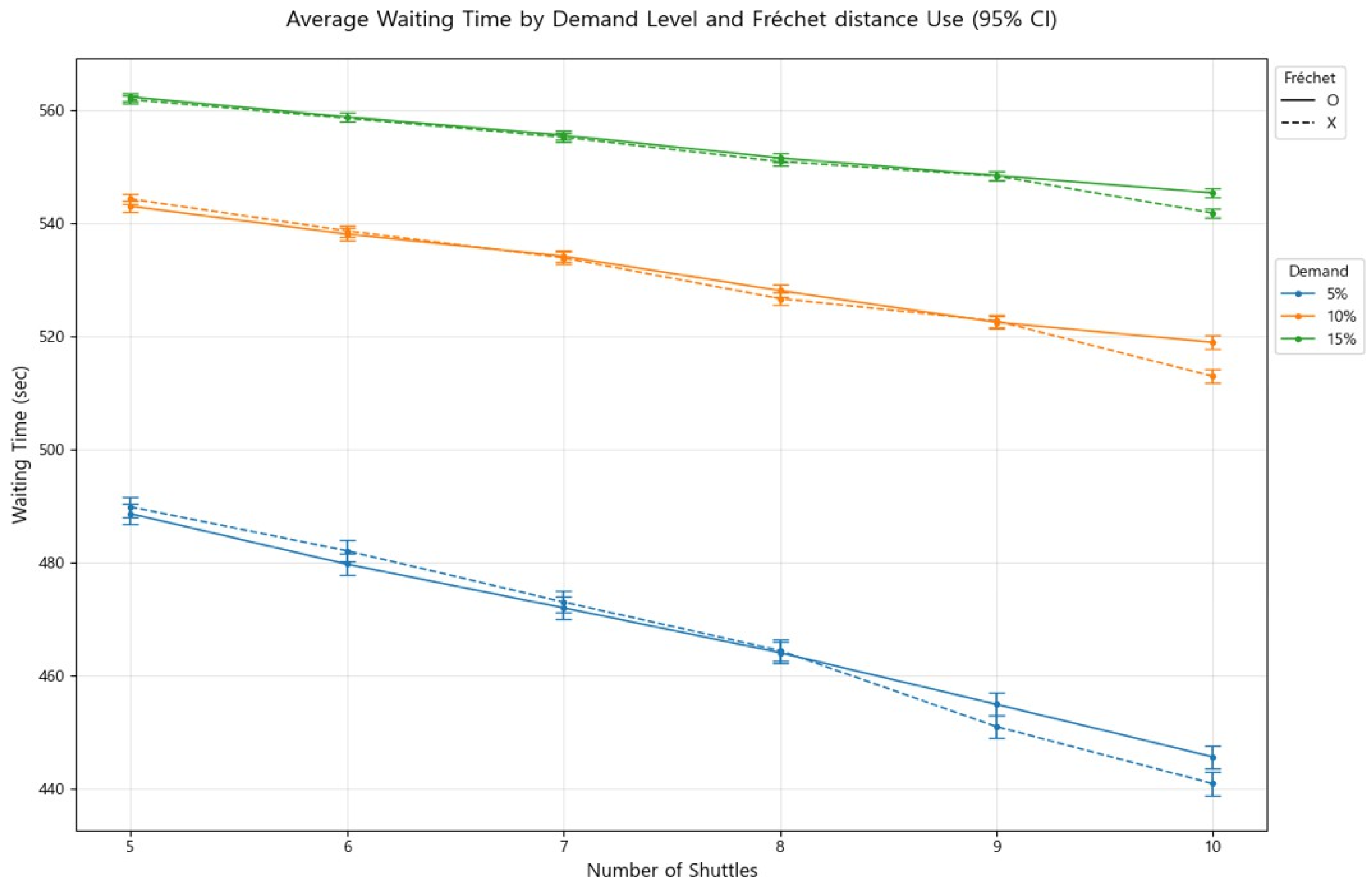
Figure 15 shows that average passenger waiting time decreases as the number of vehicles increases. The x-axis represents the fleet size, and the y-axis indicates passenger waiting time in seconds. As shown in Figure 15, the difference in average waiting time associated with applying the Fréchet distance-based algorithm is minimal, amounting to approximately 0.61 s relative to the case without the algorithm.

A clear increase in passenger waiting time is observed as the demand reflection rate rises. When the Fréchet distance-based algorithm is applied, the average waiting time increases by 63.31 s as demand increases from 5% to 10%, and by an additional 22.88 s as demand rises from 10% to 15%. This trend indicates that higher demand levels lead to longer waiting times because each shuttle must serve more requests, resulting in increased response and dispatch delays. In particular, under high-demand conditions with a limited fleet, the pool of available candidate vehicles becomes insufficient, causing some requests to experience prolonged waiting and increasing overall passenger waiting time.

Meanwhile, in scenarios with nine or more vehicles, applying the Fréchet distance-based algorithm yields an average waiting time approximately 4.33 s longer than that observed without the algorithm. This outcome is attributed to the excessive restriction of the candidate vehicle set caused by Fréchet distance filtering, which limits assignment flexibility and prevents efficient matching for certain requests. Consequently, when many candidate vehicles are available, the Fréchet distance-based algorithm may reduce matching flexibility and slightly degrade vehicle assignment performance.

4.4.2. Performance Evaluation of the Satisfaction-Based Final Vehicle Selection Algorithm

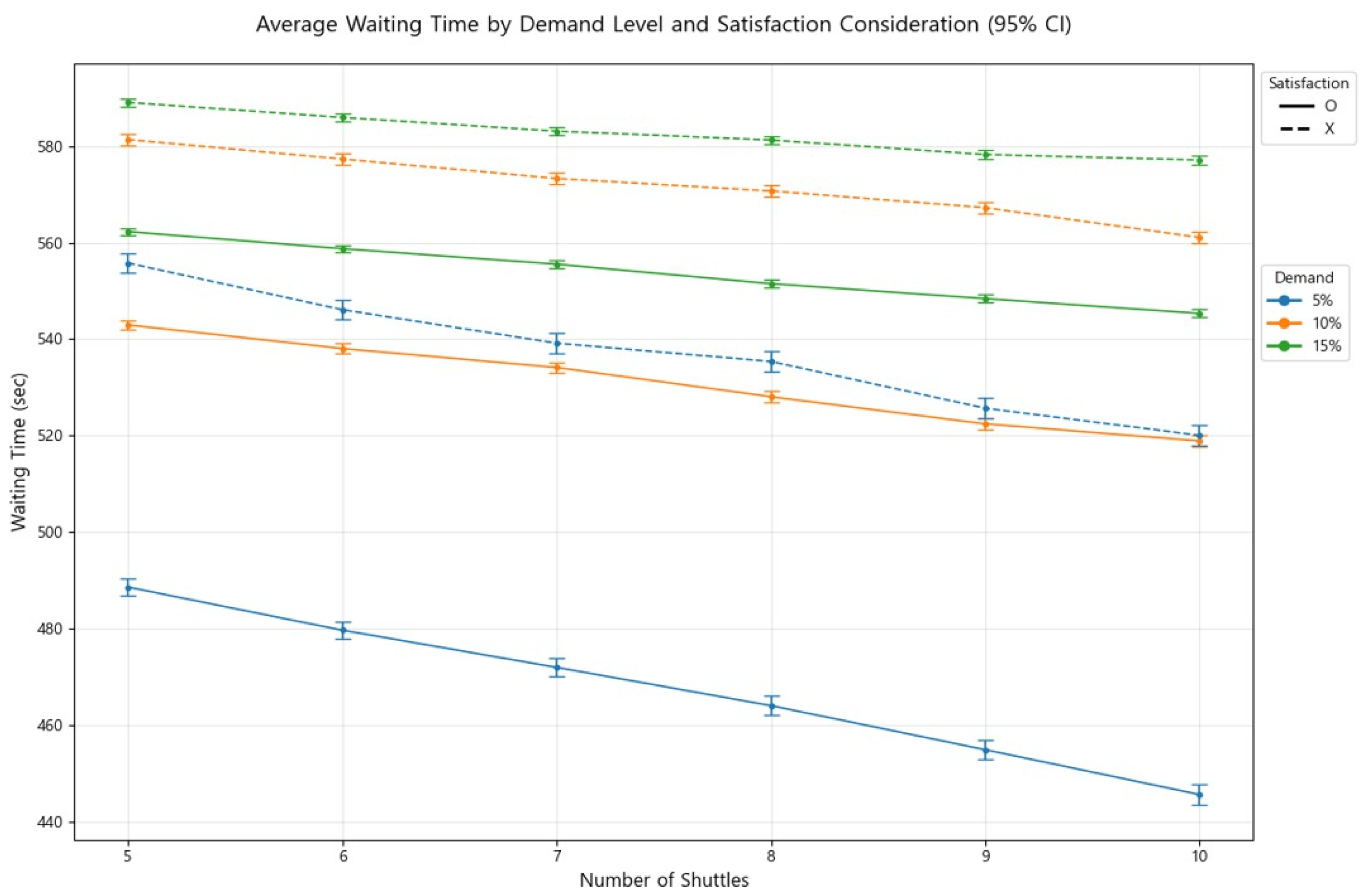
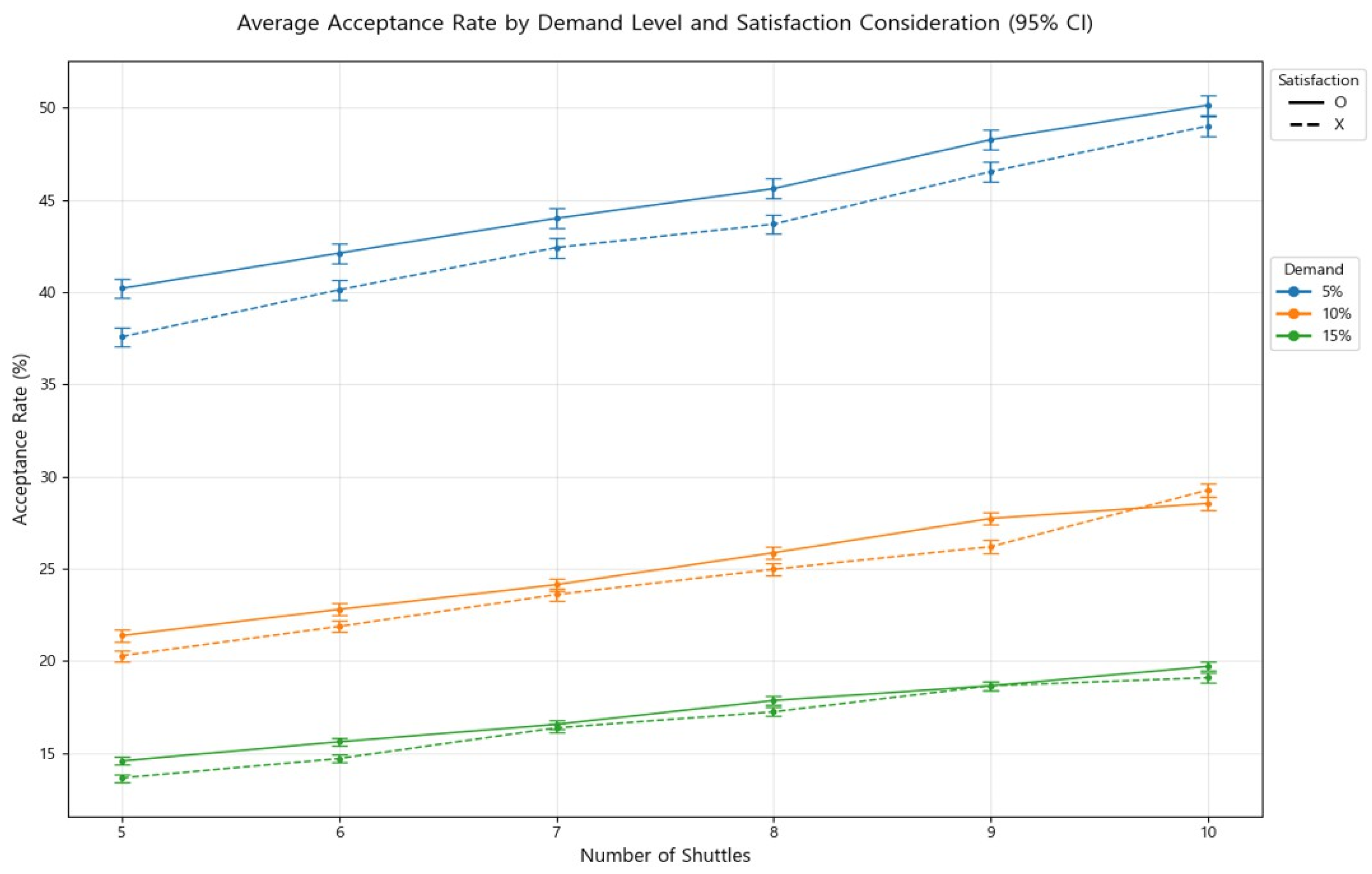
Section 4.4.2 presents the performances evaluation of the Fréchet distance-based vehicle candidate selection algorithm, the satisfaction-based final vehicle selection algorithm. The line styles and colors used in Figure 16 and Figure 17 are defined as follows: solid lines indicate cases in which the satisfaction-based final vehicle selection algorithm is applied, whereas dashed lines represent cases without the algorithm. Blue lines correspond to a demand reflection rate of 5%, orange lines to 10%, and green lines to 15% of total demand.

Figure 16 compares average passenger waiting times across different fleet sizes and demand reflection rates with and without the satisfaction-based final vehicle selection algorithm. The x-axis denotes the number of vehicles used in the simulation, and the y-axis represents the average passenger waiting time in seconds. As the fleet size increases, the average waiting time consistently decreases because more vehicles are available to serve requests. When the satisfaction-based algorithm is applied, waiting times are generally lower than in cases without satisfaction consideration. Specifically, the average waiting time is reduced by 69.58 s at a 5% demand reflection rate, by 41.09 s at 10%, and by 28.8 s at 15%. These results indicate that the satisfaction-based final vehicle selection algorithm effectively reduces passenger waiting time. This improvement occurs because vehicle assignments prioritize passengers with higher satisfaction sensitivity, thereby alleviating overall waiting burdens.

As the demand reflection rate increases, the difference in waiting time between cases with and without satisfaction consideration gradually decreases. Higher demand leads to greater spatial and temporal concentration of ride requests, limiting the number of passengers that can be served by a fixed fleet. As waiting times accumulate across more passengers, the overall average waiting time increases, reducing the relative advantage of satisfaction-based selection.

Overall, Figure 16 illustrates the performance differences in the algorithm under varying fleet sizes and demand distributions, highlighting that satisfaction-aware strategies are particularly effective when sufficient vehicle resources are available.

Figure 17 compares the shuttle acceptance rate with and without satisfaction consideration under various demand reflection rates and fleet size conditions. The x-axis represents the number of vehicles, and the y-axis shows the shuttle acceptance rate as a percentage. Across all demand reflection rates (5%, 10%, and 15%), the acceptance rate achieved with satisfaction consideration is consistently higher by approximately 1.02% than in cases without it. For example, under the 5% demand reflection scenario, approximately 13,000 requests are accepted out of about 32,000 total requests when the satisfaction-based algorithm is applied.

In contrast, only around 12,000 accepted requests without the algorithm. This represents a difference of approximately 1000 additional accepted requests. As the demand reflection rate increases, the number of passengers relative to the fixed fleet size also increases, leading to overall decreases in acceptance rates to 1.83%, 0.70%, and 0.54%, respectively. However, as the number of vehicles increases, the number of requests that can be served also rises, resulting in an average increase of 2.16% in overall acceptance rate. These results collectively demonstrate the effectiveness of the satisfaction-based vehicle selection algorithm in improving shuttle acceptance performance under varying demand and fleet size conditions.

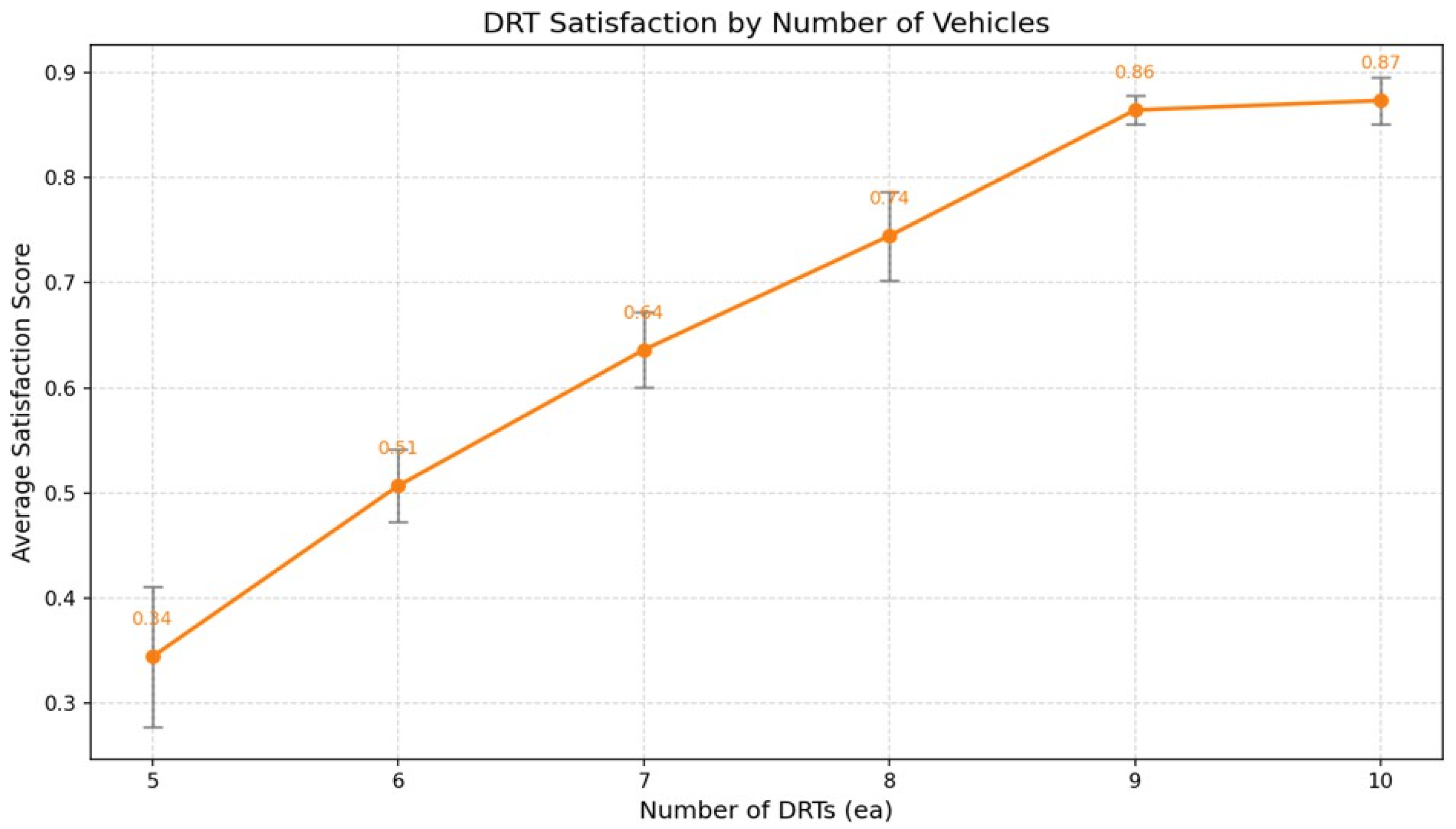
Figure 18 presents passenger satisfaction scores as a function of the number of vehicles under a 10% demand reflection rate. The x-axis denotes the number of vehicles, and the y-axis indicates the passenger satisfaction score. Overall, passenger satisfaction increases as the fleet size grows. In particular, under the 10% demand reflection condition with only five vehicles, the feasibility of serving requests varies substantially depending on passengers’ origins and destinations. Consequently, the confidence interval of satisfaction scores is relatively wide under this condition.

Furthermore, as shown in Figure 16, the reduction in passenger waiting time diminishes as the number of vehicles increases from nine to ten. Similarly, Figure 17 shows that the increase in shuttle acceptance rate decreases from 0.12 to 0.10 over the same range. Taken together, these results suggest that, under a 10% demand reflection rate, a fleet size of nine vehicles represents an optimal operating point. This analysis indicates that the simulation model operates within a reasonable and consistent range and supports the validity of the proposed framework for predicting and evaluating passenger satisfaction with respect to fleet size. It should be noted that the acceptance rate is constrained by operational factors such as vehicle capacity and route insertion feasibility. Therefore, although the acceptance rate increases as the fleet size grows, the increase is expected to gradually diminish and approach an upper bound rather than continue increasing indefinitely.

5. Conclusions

This study proposed a DEVS-based simulation framework for DRT operations and developed an integrated dispatching and routing mechanism that simultaneously considers route similarity, traffic congestion, and passenger satisfaction. By incorporating real public transportation data, dynamic passenger request locations, and modular DEVS models, the proposed framework enables realistic and scalable evaluation of DRT systems under time-varying demand conditions.

First, a unified DEVS-based simulation framework was developed to model the full DRT operational process, including passenger request generation, vehicle dispatching, route planning, and performance evaluation. The framework successfully reproduces realistic temporal and spatial demand patterns observed in real-world public transportation data. Second, the Fréchet distance-based candidate vehicle selection (FD-CVS) algorithm effectively reduces computational complexity by limiting the search space for vehicle assignment. Simulation results demonstrate that the average wall time decreases by 9.57 s, 23.59 s, and 44.38 s under demand rates of 5%, 10%, and 15%, respectively, while maintaining comparable passenger waiting-time performance. Third, the satisfaction-aware vehicle assignment (SA-VA) algorithm significantly improves passenger-oriented service quality. By explicitly accounting for passenger waiting time and in-vehicle travel time, the algorithm reduces average waiting time by up to 69.58 s and increases the shuttle acceptance rate by approximately 1.02% compared with cases in which passenger satisfaction is not considered. Finally, the experimental results reveal clear trade-offs between computational efficiency and assignment flexibility. While FD-CVS is highly effective under high-demand and limited-fleet conditions, excessive candidate filtering may slightly degrade performance when sufficient vehicle resources are available.

Overall, the proposed framework provides a practical decision-support tool for DRT planning and evaluation by integrating multiple operational objectives within a single simulation environment. It is particularly well suited for analyzing large-scale DRT systems in which real-time responsiveness and passenger satisfaction must be balanced. However, in this study traffic conditions are represented using network travel-time information and congestion-aware routing, and fully dynamic traffic variations such as traffic incidents or rapidly changing congestion patterns are not explicitly modeled. Future research directions include conducting sensitivity analyses of key algorithmic parameters, such as candidate set size and satisfaction threshold values; incorporating more detailed and dynamically calibrated traffic models to address the simplified representation of traffic patterns used in the current simulation framework; integrating more detailed and dynamically calibrated traffic congestion models; extending the framework to large-scale networks, multi-depot systems, and vehicle repositioning strategies; and incorporating learning-based dispatching and routing methods, such as reinforcement learning, validated with additional real-world operational datasets.

References

1. Cordeau, J.-F.; Laporte, G. The dial-a-ride problem: Models and algorithms. Ann. Oper. Res. 2007, 153, 29–46. [Google Scholar] [CrossRef]
2. Parragh, S.N.; Doerner, K.F.; Hartl, R.F. A survey on pickup and delivery problems: Part II—Transportation between pickup and delivery locations. J. Für Betriebswirtschaft 2008, 58, 81–117. [Google Scholar] [CrossRef]
3. Quadrifoglio, L.; Li, X. A methodology to derive the critical demand density for designing and operating feeder transit services. Transp. Res. Part B 2009, 43, 922–935. [Google Scholar] [CrossRef]
4. Navidi, Z.; Ronald, N.; Winter, S. Comparison between ad-hoc demand responsive and conventional transit: A simulation study. Public Transp. 2018, 10, 147–167. [Google Scholar] [CrossRef]
5. Alonso-Mora, J.; Samaranayake, S.; Wallar, A.; Frazzoli, E.; Rus, D. On-demand high-capacity ride-sharing via dynamic trip-vehicle assignment. Proc. Natl. Acad. Sci. USA 2017, 114, 462–467. [Google Scholar] [CrossRef]
6. Cordeau, J.-F.; Laporte, G.; Savelsbergh, M.W.P. A branch-and-cut algorithm for the dial-a-ride problem. Oper. Res. 2006, 54, 573–586. [Google Scholar] [CrossRef]
7. Horn, M.E.T. Fleet scheduling and dispatching for demand-responsive passenger services. Transp. Res. Part C 2002, 10, 35–63. [Google Scholar] [CrossRef]
8. Ronald, N.; Thompson, R.; Winter, S. Simulating demand-responsive transportation: A review of agent-based approaches. Transp. Rev. 2015, 35, 404–421. [Google Scholar] [CrossRef]
9. Oh, S.; Seshadri, R.; Le, D.-T.; Zegras, P.C.; Ben-Akiva, M.E. Evaluating automated demand responsive transit using microsimulation. IEEE Access 2020, 8, 82551–82561. [Google Scholar] [CrossRef]
10. Hyytiä, E.; Penttinen, A.; Sulonen, R. A stochastic model for a vehicle in a dial-a-ride system. Oper. Res. Lett. 2010, 38, 432–435. [Google Scholar] [CrossRef]
11. Stiglic, M.; Agatz, N.; Savelsbergh, M.; Gradisar, M. The benefits of meeting points in ride-sharing systems. Transp. Res. Part B 2015, 82, 36–53. [Google Scholar] [CrossRef]
12. Hyytiä, E.; Penttinen, A.; Sulonen, R. Non-Myopic Vehicle and Route Selection in Dynamic DARP with Travel Time and Workload Objectives. Comput. Oper. Res. 2012, 39, 3021–3030. [Google Scholar] [CrossRef]
13. Ichoua, S.; Gendreau, M.; Potvin, J.-Y. Vehicle dispatching with time-dependent travel times. Eur. J. Oper. Res. 2003, 144, 379–396. [Google Scholar] [CrossRef]
14. Macal, C.M.; North, M.J. Tutorial on agent-based modeling and simulation. J. Simul. 2010, 4, 151–162. [Google Scholar] [CrossRef]
15. Liu, Y.; Bansal, P.; Daziano, R.; Samaranayake, S. A framework to integrate mode choice in the design of mobility-on-demand systems. Transp. Res. Part C Emerg. Technol. 2019, 105, 648–665. [Google Scholar] [CrossRef]
16. Dong, W.; Wang, N.; Dong, Y.; Cao, J. Examining the nonlinear and interactive effects of built environment characteristics on travel satisfaction. J. Transp. Geogr. 2025, 123, 104111. [Google Scholar] [CrossRef]
17. Bongiovanni, C.; Kaspi, M.; Geroliminis, N. The electric autonomous dial-a-ride problem. Transp. Res. Part B 2019, 122, 436–456. [Google Scholar] [CrossRef]
18. Ma, S.; Zheng, Y.; Wolfson, O. T-share: A large-scale dynamic taxi ridesharing service. IEEE Trans. Knowl. Data Eng. 2015, 27, 1782–1795. [Google Scholar] [CrossRef]
19. Agatz, N.; Erera, A.; Savelsbergh, M.; Wang, X. Optimization for dynamic ride-sharing: A review. Eur. J. Oper. Res. 2012, 223, 295–303. [Google Scholar] [CrossRef]
20. Zigrand, L.; Calvo, R.W.; Traversi, E.; Alizadeh, P. A scalable combinatorial Benders decomposition for the stochastic dial-a-ride problem. Transp. Res. Part C Emerg. Technol. 2024, 163, 104624. [Google Scholar] [CrossRef]
21. Park, J.; Lee, J.; Kim, J.; Chung, J.H. An optimization model of on-demand mobility services with spatial heterogeneity in travel demand. Transp. Res. Part C Emerg. Technol. 2023, 153, 104229. [Google Scholar] [CrossRef]
22. Wu, W.; Zhang, Z.; Lu, K.; Ren, J. Dynamic demand-responsive transit scheduling with time-dependent travel times: A joint supply and demand management approach. Transp. Res. Part E Logist. Transp. Rev. 2025, 202, 104232. [Google Scholar] [CrossRef]
23. Han, S.-W.; Moon, S.; Kim, D.-K. Multi-objective optimization of demand responsive transit operations based on dynamic passenger requests using maximum time delay rate. J. Public Transp. 2024, 26, 100108. [Google Scholar] [CrossRef]
24. Dastani, Z.; Koosha, H.; Karimi, H.; Moghaddam, A.M. User preferences in ride-sharing mathematical models for enhanced matching. Sci. Rep. 2024, 14, 27338. [Google Scholar] [CrossRef]
25. Lu, C.; Wu, Y.; Yu, S. A sample average approximation approach for the stochastic dial-a-ride problem on a multi-graph with user satisfaction. Eur. J. Oper. Res. 2022, 302, 1031–1044. [Google Scholar] [CrossRef]
26. Ghandeharioun, Z.; Kouvelas, A. Real-time ridesharing operations for on-demand capacitated systems considering dynamic travel time information. Transp. Res. Part C Emerg. Technol. 2023, 151, 104115. [Google Scholar] [CrossRef]
27. Cho, S.-W.; Lim, Y.-H.; Ju, S.-H.; Seo, K.-M. Analyzing New Operation Strategy of Demand-Responsive Transports Using Discrete-Event Simulation Framework. Systems 2025, 13, 303. [Google Scholar] [CrossRef]
28. Obonguta, F.; Lee, J.; Mizutani, D. Simultaneous optimization of road intervention and overloading penalty policies for user cost minimization. Transp. Res. Interdiscip. Perspect. 2026, 36, 101849. [Google Scholar] [CrossRef]
29. Kogler, C.; Rauch, P. Discrete event simulation of multimodal and unimodal transportation in the wood supply chain: A literature review. Silva Fenn. 2018, 52, 4. [Google Scholar] [CrossRef]
30. Jäger, B.; Brickwedde, C.; Lienkamp, M. Multi-agent simulation of a demand-responsive transit system operated by autonomous vehicles. Transp. Res. Rec. 2018, 2672, 764–774. [Google Scholar] [CrossRef]
31. Seo, K.M.; Choi, C.; Kim, T.G.; Kim, J.H. DEVS-based combat modeling for engagement-level simulation. Simulation 2014, 90, 129–142. [Google Scholar] [CrossRef]
32. Kim, J.H.; Seo, K.-M.; Lee, T.-E.; Choi, B.-W. Achieving new insights into combat engagement analysis via simulation-based sequential experimentation. Mil. Oper. Res. 2018, 23, 51–80. [Google Scholar]
33. Sung, J.-H.; Ju, S.-H.; Cho, S.-W.; Joo, H.-J.; Seo, K.-M.; Kang, B.-G. Modeling and exploratory analysis of discrete event simulations for optimizing overhead hoist transport systems and logistics in semiconductor manufacturing. Mathematics 2025, 13, 1167. [Google Scholar] [CrossRef]
34. Zeigler, B.P.; Kewley, R.; Wainer, G. DEVS closure under coupling, universality, and uniqueness: Enabling simulation and software interoperability from a system-theoretic foundation. Computers 2025, 14, 514. [Google Scholar] [CrossRef]
35. Chen, J.; Zhang, S.; Xu, W. Scalable prediction of heterogeneous traffic flow with enhanced non-periodic feature modeling. Expert Syst. Appl. 2025, 294, 128847. [Google Scholar] [CrossRef]
36. Oberle, W. Monte Carlo Simulations: Number of Iterations and Accuracy; Technical Note ARL-TN-0684; U.S. Army Research Laboratory: Adelphi, MD, USA, 2015.
37. Bicher, M.; Wastian, M.; Brunmeir, D.; Popper, N. Review on Monte Carlo simulation stopping rules: How many samples are really enough? Simul. Notes Eur. 2022, 32, 1–8. [Google Scholar] [CrossRef]
38. Sarker, V.K.; Nguyen Gia, T.; Ben Dhaou, I.; Westerlund, T. Smart parking system with dynamic pricing, edge-cloud computing and LoRa. Sensors 2020, 20, 4669. [Google Scholar] [CrossRef] [PubMed]
39. Ansari Esfeh, M.; Wirasinghe, S.C.; Saidi, S.; Kattan, L. Waiting time and headway modelling for urban transit systems—A critical review and proposed approach. Transp. Rev. 2021, 41, 141–163. [Google Scholar] [CrossRef]
40. Wong, R.C.P.; Yang, L.; Szeto, W.Y. Comparing passengers’ satisfaction with fixed-route and demand-responsive transport services: Empirical evidence from public light bus services in Hong Kong. Travel Behav. Soc. 2023, 32, 100583. [Google Scholar] [CrossRef]
41. Webb, A.; Kumar, P.; Khani, A. Estimation of passenger waiting time using automatically collected transit data. Public Transp. 2020, 12, 299–311. [Google Scholar] [CrossRef]
42. Lu, C.; Kühnel, N. To wait or to cruise: The trade-off between waiting time and detours for service efficiency in ride-pooling systems. Case Stud. Transp. Policy 2025, 21, 101499. [Google Scholar] [CrossRef]
43. Hrastovec, M.; Solina, F. Prediction of aircraft performances based on data collected by air traffic control centers. Transp. Res. Part C Emerg. Technol. 2017, 73, 167–182. [Google Scholar] [CrossRef]
44. Novak, J.; Rebernjak, B. Monte Carlo simulation studies of reliability in psychometrics: A methodological review. Adv. Methodol. Stat. 2024, 19, 61–128. [Google Scholar] [CrossRef]
45. Cho, S.-W.; Seo, K.-M.; Yun, J.-M.; Kang, B.-G. Simulation-Based Analysis for Verifying New Certification Standards of Smart LED Streetlight Systems. Mathematics 2024, 12, 657. [Google Scholar] [CrossRef]
46. Sun, H.; Cao, D.; Liu, Z. Climate policy uncertainty and corporate supply chain stability. Int. Rev. Econ. Financ. 2025, 104, 104581. [Google Scholar] [CrossRef]
47. Li, H.; Kim, S. Efficient route planning for real-time demand-responsive transit. Comput. Mater. Contin. 2024, 79, 473–492. [Google Scholar] [CrossRef]
48. Zhang, Y.; Gao, L.; Zhao, X.; Ni, A. Data-driven modeling of demand-responsive transit: Evaluating sustainability across urban, rural, and intercity scenarios. Systems 2025, 13, 1080. [Google Scholar] [CrossRef]
49. Tandan, S.; Anthony, A.M.; Kim, H. Investigating factors affecting request matching in demand-responsive transit service with different fleet sizes using a decision tree model. Appl. Sci. 2025, 15, 12134. [Google Scholar] [CrossRef]
50. Lyu, Z.; Pons, D.; Palliparampil, G.; Zhang, Y. Optimising Urban Freight Logistics Using Discrete-Event Simulation and Cluster Analysis: A Stochastic Two-Tier Hub-and-Spoke Architecture Approach. Smart Cities 2023, 6, 2347–2366. [Google Scholar] [CrossRef]
51. Zhang, J.; Guo, R.; Li, W. Research on Dynamic Scheduling and Route Optimization Strategy of Flex-Route Transit Considering Travel Choice Preference of Passenger. Systems 2024, 12, 138. [Google Scholar] [CrossRef]
52. Zhang, C.; Xie, Y.; Gartner, N.H.; Stamatiadis, C.; Arsava, T. AM-Band: An Asymmetrical Multi-Band Model for Arterial Traffic Signal Coordination. Transp. Res. Part C Emerg. Technol. 2015, 58, 515–531. [Google Scholar] [CrossRef]
Figure 1. Differences between the target system and conventional transportation modes.
Mathematics 14 01099 g001
Figure 2. DRT system assignment process.
Mathematics 14 01099 g002
Figure 3. Proposed simulation framework.
Mathematics 14 01099 g003
Figure 4. Simulation model structure for DRT operations.
Mathematics 14 01099 g004
Figure 5. Schedule Manager atomic model structure (“!”: output port, “?”: input port for event message transmission, “@”: conditional statement).
Mathematics 14 01099 g005
Figure 6. Dispatching & Routing Manager atomic model structure (“!”: output port, “?”: input port for event message transmission, “@”: conditional statement).
Mathematics 14 01099 g006
Figure 7. Fréchet Distance-Based Candidate Vehicle Selection process.
Mathematics 14 01099 g007
Figure 8. Traffic volume estimation process.
Mathematics 14 01099 g008
Figure 9. Satisfaction-Aware Vehicle Assignment process.
Mathematics 14 01099 g009
Figure 10. Experimental design framework.
Mathematics 14 01099 g010
Figure 11. Number of demand occurrences by time zone.
Mathematics 14 01099 g011
Figure 12. Visualization of demand generation locations (blue dots: existing bus stops; red dots: dynamic demand nodes).
Mathematics 14 01099 g012
Figure 13. Differences between expected and actual boarding and waiting times by number of vehicles.
Mathematics 14 01099 g013
Figure 14. Average wall time by demand level as a function of the number of vehicles.
Mathematics 14 01099 g014
Figure 15. Average passenger waiting time by demand level as a function of the number of vehicles.
Mathematics 14 01099 g015
Figure 16. Average waiting time by demand level and satisfaction consideration.
Mathematics 14 01099 g016
Figure 17. Average acceptance rate by demand level and satisfaction consideration.
Mathematics 14 01099 g017
Figure 18. Average satisfaction score by number of DRT vehicles.
Mathematics 14 01099 g018