Analytical Perspectives and Numerical Simulations of a Mathematical Model for Spatiotemporal Dynamics of Citrus Greening

Abstract

In this study, we propose a compartmental mathematical model that considers two interacting populations (citrus plants and insect vectors) and investigate the transmission dynamics of Huanglongbing in citrus crops. This disease is caused by the bacterium Candidatus Liberibacter asiaticus and is vectored by the psyllid Diaphorina citri. The disease is modeled under the following three main assumptions: there is vital dynamics with constant recruitment rates of citrus plants, the force of infection in both populations is a spatially dependent function varying with geographic location, and there is a spatial displacement of the vectors. In the main results of the paper, we formulate a coupled ordinary and partial differential equation system with initial and zero flux boundary conditions, establish the existence and uniqueness of solutions to the proposed model by applying semigroup theory, and introduce a numerical approximation of the system. Moreover, we develop a stability and persistence analysis. From the analytical point of view, we calculate the basic reproduction number $R_0$ and prove three facts: the disease-free equilibrium is globally asymptotically stable when $R_0<1$; the disease-free equilibrium is globally asymptotically stable when $R_0>1$; and the hybrid system exhibits uniform persistence of infection when $R_0>1$. In addition, we present some numerical examples.

1. Introduction

Within the framework of the United Nations report on the Sustainable Development Goals, it is emphasized that, since 2015, both hunger and food insecurity have gained increasing relevance as global challenges, reflecting a significant rise in their impact and in the urgency of addressing them [1]. Approximately 80% of the food consumed daily is derived from plants, which also produce 98% of the oxygen that is essential for human respiration. Therefore, plant health plays an essential role in promoting sustainable agricultural development, which is indispensable for ensuring that the nutritional needs of a growing global population are met, not only by 2050 but also beyond this horizon [2].

Citrus crops (including lemons, oranges, and mandarins) are not only consumed directly but also serve as inputs for various industrial processes, particularly in the food, pharmaceutical, and biotechnology sectors. The most relevant processes include essential oil extraction, pectin production, flavonoid recovery, enzyme production, and juice processing [3,4].

Currently, citrus fruits are cultivated in more than 140 countries worldwide, with an annual production exceeding 122 million tons, underscoring the great economic importance of this crop [5,6,7]. Throughout their lifecycle, citrus plants are vulnerable to numerous pests and diseases. Among these, citrus greening, also known as Huanglongbing (HLB), stands out as a particularly destructive disease that has severely affected the global citrus industry over the past few decades [8]. This disease is caused by the bacterium Candidatus Liberibacter asiaticus (Ca. L.), which is transmitted via the psyllid vector Diaphorina citri (D.) [9].

The bacterium Ca. L. establishes and proliferates in the phloem of host plants, where it obstructs the transport of nutrients and water, leading to a reduction in vegetative productivity. Once the bacterium colonizes the infected shoots, it spreads throughout the canopy of the tree, increasing physiological damage [10]. In this context, the insect vector D. plays a key role in the epidemiology of the disease: by feeding on infected citrus tissues, it acquires the pathogen and transmits it to new plants, remaining infectious throughout its entire lifespan [11]. Symptoms typically manifest in leaves and fruits, producing bitter misshapen citrus. Diagnosis is challenging as symptoms may be mistaken for other conditions, such as chlorosis or nutritional deficiencies—including those related to nitrogen, zinc, magnesium, or manganese. Therefore, it is essential to conduct periodic monitoring of citrus crops to detect the pathogen in a timely manner [12]. There are surveillance and research methods for some specific regions, including the following: Brazil [13,14], México [15], the USA [16,17,18], and Europe [19]; a more complete report is constructed by COSAVE [11], D. which includes other regions, like Argentina, Bolivia, Paraguay, and Uruguay.

Nowadays, there is extensive research on the influence of seasonality on plant disease transmission using mathematical modeling [20,21,22]. For instance, seasonal variations in temperature and rainfall can alter vector population dynamics and host susceptibility, thereby modulating the rate of pathogen spread. In this context, several contributions [22,23,24] investigate the existence and uniqueness of solutions to models of disease dissemination within ecosystems under biologically plausible assumptions, such as bounded growth of host populations, limited carrying capacity, and realistic transmission rates that vary periodically with environmental conditions. Additionally, the authors in Coronel et al. [25] propose a generalized Susceptible–Infectious–Susceptible compartmental model and examine the existence of positive periodic solutions via the application of Mawhin’s coincidence degree theorem.

In concrete terms, for HLB, mathematical modeling has emerged as a valuable and essential tool for understanding its epidemiological characteristics from the point of view of the change over time in tree and psyllid populations, as documented in [26]. A representative list of the currently existing mathematical models includes the following [14,15,27,28,29,30,31,32,33,34,35,36,37,38,39,40,41,42,43,44,45,46,47,48,49,50,51,52,53,54,55,56,57,58,59,60,61,62], which can be arranged into three groups:

(i) 

We consider the works [18,27,28,29,30], where some mathematical models based on elementary functions are developed. For instance, in [27], some geometric relations are introduced for early recognition of infected trees; in [18,28], discrete models based on a binomial relation are introduced to fit the population trees; in [29], the populations are approximated by an exponential function; and, in [30], a recurrence relation for population trees is considered.

(ii) 

Our focus lies in mathematical models based on systems of ordinary differential equations [31,32,33,34,35,36,37,38,39,40,41,42,43,44,45,46,47,48,49,50,51,52]. In those works, the authors apply the compartmental methodology, the approach in which tree and psyllid populations are grouped by epidemiological category (susceptible, recovered, asymptomatic, or other), and applying a mass balance establishes that the populations in each category satisfy an ordinary differential equation, which is coupled with the equations of the other categories as a consequence of the interaction of the populations of the different categories considered. The most notable and common characteristic is that the system unknowns are time-dependent continuous functions that model the populations of the different categories over time.

(iii) 

Three kinds of models are obtained by the modification of the compartmental methodology to incorporate some biological properties. First, in the articles [14,53,54,55,56], the authors are focused on the application of a compartmental methodology by considering that the populations of some categories are approximated by time-dependent functions with delay, incorporating in the mathematical models some biological characteristics, such as incubation period, resulting in delay differential systems as the mathematical models. Second, the impulsive differential system models define another modification of ordinary differential systems originating in the compartmental methodology [57,58], in which the unknowns are time-dependent functions with discontinuities that model abrupt changes at specific times as a consequence of some characteristics, such as births or deaths due to fumigation.

The disadvantage or limitation of the mathematical models constructed using the compartmental methodology is the assumption that the populations of the different categories are homogeneously distributed in space, which is not satisfied by real populations. Some improvements to account for the heterogeneous behavior of populations are given in [59,60,63,64], where fractional derivatives (instead of ordinary derivatives) and mathematical diffusion are considered, respectively. Therefore, it is very necessary to research the incorporation of population heterogeneity into mathematical models based on the compartmental methodology.

In this paper, motivated by the preceding discussion, we focus on introducing and analyzing a mathematical model for HLB transmission in citrus and psyllid populations that accounts for heterogeneity by incorporating vector spatial displacement. More specifically, we state three main aims: the construction of a mathematical model using the compartmental methodology and the mathematical diffusion concept, the formal analysis of the proposed mathematical model in an appropriate framework, and the numerical approximation of the model. In concordance with our aims, we obtain the following results. First, we introduce a mathematical model consisting of a system of six equations: three ordinary differential equations and three partial differential equations. The unknowns in the ordinary differential equations and the partial differential equations are the populations of the three categories of trees and the three categories of vectors, respectively. Moreover, we derive boundary conditions that model the absence of vector population immigration or migration across the domain boundary. We analyze the mathematical model by applying the semigroup theory and introduce a stability analysis. In the case of the well-posedness analysis, we get the existence, uniqueness, positivity and boundedness of the strong solution. Meanwhile, in the case of the stability analysis, we introduce a definition of the basic reproduction number and provide some results for the uniform persistence. Third, to demonstrate the applicability of our framework, we present two numerical examples that illustrate distinct epidemiological scenarios and highlight how the proposed model can be used to evaluate the impact of different assumptions and interventions on disease dynamics.

2. Preliminaries and Mathematical Model Formulation

In this section, we introduce the mathematical model by applying the compartmental methodology. We distinguish two steps: model assumptions and mass balance with spatial displacement of vectors. Moreover, to make this paper self-contained, we include necessary definitions and background on reaction–diffusion concepts at the beginning and provide remarks on the mathematical model analysis at the end of the section.

2.1. Reaction–Diffusion Equations and Related Mathematical Concepts

We introduce the reaction–diffusion concepts by following the presentation given in [65,66,67]. To precisely define the mathematical diffusion concept, we consider that the density of an individual (organism or particle) is given by $u=u(x,t)$ and assume that ${\mathsf{\Omega }}^{\prime }\subset \mathsf{\Omega }\subset {\mathbb{R}}^d$ is a smooth subregion. Then, by the mass conservation principle, we have that the rate of change of the total quantity within ${\mathsf{\Omega }}^{\prime }$ is equal to the negative of the net flux through its boundary $\partial {\mathsf{\Omega }}^{\prime }$:

$$\begin{array}{c}\hfill {\displaystyle \frac{d}{dt}}{\int }_{{\mathsf{\Omega }}^{\prime }}u(x,t)dx=-{\int }_{\partial {\mathsf{\Omega }}^{\prime }}\mathbf{F}·\mathbf{n}dS,\end{array}$$

(1)

where $\mathbf{F}$ is the flux density and $\mathbf{n}$ is the unit outer normal vector to $\partial {\mathsf{\Omega }}^{\prime }$. Using the fact that ${\mathsf{\Omega }}^{\prime }$ is arbitrary and applying the divergence theorem, we deduce that (1) is equivalent to the following partial differential equation:

$$\begin{array}{c}\hfill {\displaystyle \frac{\partial u}{\partial t}}=-\mathrm{div}\left(\mathbf{F}\right),\end{array}$$

(2)

where $\mathrm{div}$ is the divergence operator defined as $\mathrm{div}\left(\mathbf{F}\right)={\partial }_{x_1}{\mathbf{F}}_1+\dots +{\partial }_{x_d}{\mathbf{F}}_d$. Let us consider that the gradient of u is defined by $\nabla u=({\partial }_{x_1}u,\dots ,{\partial }_{x_d}u)$. A proposal to model the flux density is given by the “Fick law”, which states that “$\mathbf{F}$ is proportional to the gradient u, but points in the opposite direction (since the flow is from regions of higher to lower concentration)” or, equivalently,

$$\begin{array}{c}\hfill \mathbf{F}=-D\nabla u,\end{array}$$

(3)

where D is the diffusion coefficient. Let us consider the Laplacian of u defined by $\Delta u={\partial }_{x_1^2}^{2}u+\dots +{\partial }_{x_d^2}^2{u}_d$. Replacing (3) in (2) and using the identity $\mathrm{div}(\nabla u)=\Delta u$, we get

$$\begin{array}{c}\hfill {\displaystyle \frac{\partial u}{\partial t}}=D\Delta u,\end{array}$$

(4)

which is called the diffusion equation. In many situations, instead of (1), we have the balance form

$$\begin{array}{c}\hfill {\displaystyle \frac{d}{dt}}{\int }_{{\mathsf{\Omega }}^{\prime }}u(x,t)dx=-{\int }_{\partial {\mathsf{\Omega }}^{\prime }}\mathbf{F}·\mathbf{n}dS+{\int }_{{\mathsf{\Omega }}^{\prime }}R(x,t,u)dx,\end{array}$$

(5)

with R the reaction function. Hence, by similar arguments, we deduce the partial differential equation

$$\begin{array}{c}\hfill {\displaystyle \frac{\partial u}{\partial t}}=D\Delta u+R(x,t,u),\end{array}$$

(6)

which is called the reaction–diffusion equation.

2.2. Mathematical Model Step 1: Model Assumptions

We consider that the epidemic event emerges from the interaction between two populations: citrus plants and psyllids, called the host and vector populations, respectively. We consider the assumptions for each population and simultaneously introduce the notation needed to define the model as follows:

(P0) 

Citrus plants infected with HLB do not recover. The total citrus population (C) is divided into three compartments: susceptible citrus ($S_c$), consisting of healthy plants vulnerable to infection; latent citrus ($L_c$), comprising plants that have been inoculated by vectors but in which the pathogen population is not yet sufficient to be acquired or transmitted; and diseased citrus ($I_c$), representing plants in which the pathogen has reached a threshold level that allows acquisition by vectors. This distinction reflects the biological reality that plants may harbor the pathogen without immediately serving as a source of inoculum.

(P1) 

The citrus population is subject to vital dynamics. Recruitment or planting is modeled by the function $\theta$, while natural mortality associated with HLB is denoted by ${\alpha }_c$. This assumption reflects the agricultural practice of continuous planting and the impact of both natural senescence and disease pressure on orchard sustainability.

(P2) 

Susceptible citrus plants enter the latent class when inoculated by infected vectors. The transmission force from vectors to citrus is modeled by the function $\phi \left(x\right)$, which represents the rate at which susceptible plants become infected per unit of time depending on the spatial location x. This captures the biological mechanism whereby pathogen inoculation occurs during vector feeding.

(P3) 

Latent citrus plants progress to the diseased class at a rate $k_1$ once the pathogen population within the plant reaches a sufficient threshold for acquisition by vectors. This assumption reflects the biological delay between initial inoculation and the establishment of a pathogen load capable of sustaining transmission.

(V0) 

The adult psyllid population $\left(V\right)$ is structured into three epidemiological states: unexposed vectors ($S_v$), representing adult psyllids that have not yet acquired the pathogen; acquiring vectors ($E_v$), consisting of psyllids that have fed on diseased citrus plants but in which the pathogen has not yet completed the acquisition process; and infective vectors ($I_v$), representing psyllids that have successfully acquired the pathogen and are capable of transmitting it to healthy citrus plants. This classification reflects the biological distinction between acquisition and transmission phases in vector–pathogen interactions.

(V1) 

The natural mortality rate of vectors is denoted by $\mu$, while ${\mu }^{★}$ represents the mortality rate resulting from control strategies applied to the vector population. These parameters capture both the baseline lifespan of psyllids and the impact of management interventions.

(V2) 

Acquisition occurs when unexposed vectors feed on diseased citrus plants. The force of acquisition from citrus to vector is modeled by the function $\psi \left(x\right)$, which depends on the spatial variable x and represents the rate at which psyllids acquire the pathogen during feeding.

(V3) 

Vectors in the acquisition phase ($E_v$) progress to the infective state ($I_v$) at a rate $k_2$ once the pathogen has been successfully established within the insect. This transition reflects the biological delay between initial feeding and the ability to transmit the pathogen.

(V4) 

Once psyllids reach the infective state, they remain capable of transmitting the pathogen for the remainder of their lifespan. This assumption is consistent with the biology of HLB transmission, where vectors do not lose infectivity once acquisition has occurred.

(V5) 

The spatial spread of the disease is driven by vector diffusion, representing psyllid movement across space. Diffusion captures two complementary processes: long-distance dispersal of infective psyllids between orchards and short-distance movement within orchards from plant to plant. These two scales of movement jointly determine the spatial dynamics of HLB transmission.

(V6) 

Throughout the period under consideration, we assume that the psyllid population does not emigrate from or immigrate into the study domain. This assumption isolates the dynamics within the spatial region of interest.

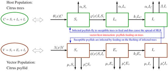
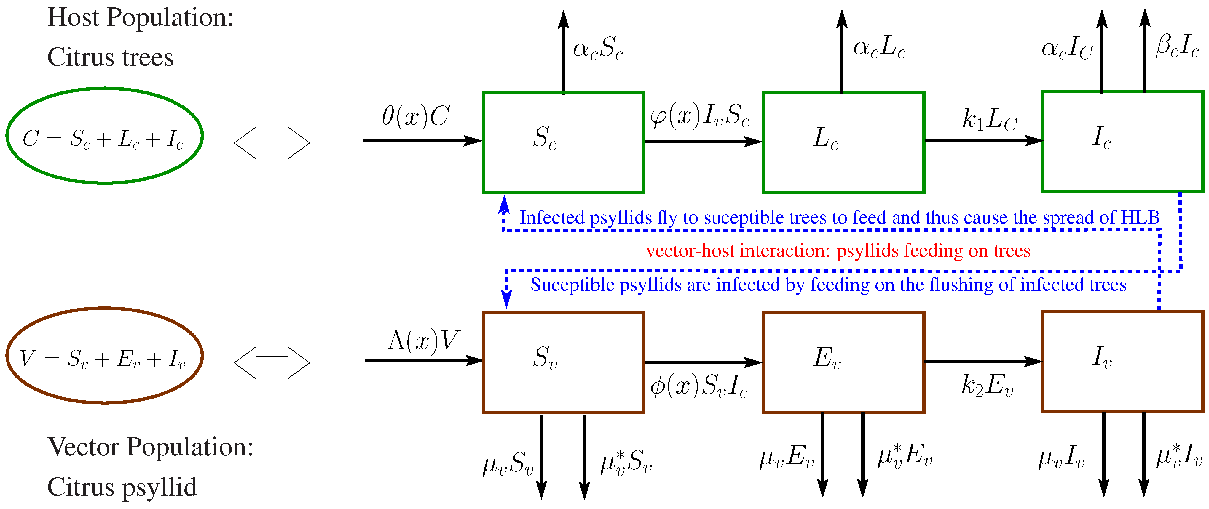
The assumptions (P0)–(P3) and (V0)–(V4), which are considered to describe the disease transmission dynamics in citrus plants as well as the spatiotemporal dynamics of the vector population, are schematically represented in Figure 1. Moreover, to clarify the mathematical formulation, we summarize the main state variables and parameters involved in the citrus–vector epidemic model in

Table 1. Summary of the notation for variables and parameter definitions used in the assumptions (P0)–(P3) and (V0)–(V4) (see Figure 1 for a summary and schematic presentation).

Variable/Parameter	Description	Unit
Host Population
C	Total citrus population	Population size
$S_c$	Healthy citrus plants (unexposed)	Population size
$L_c$	Latent citrus plants (inoculated but not yet a source of inoculum)	Population size
$I_c$	Diseased citrus plants (pathogen load sufficient for vector acquisition)	Population size
Vector Population
V	Total adult psyllid population	Population size
$S_v$	Unexposed adult vectors (not yet acquired the pathogen)	Population size
$E_v$	Acquiring adult vectors (fed on diseased citrus, pathogen not yet transmissible)	Population size
$I_v$	Infective adult vectors (pathogen acquired, capable of transmission)	Population size
Parameters
$\theta$	Citrus recruitment/planting rate	year−1
$\Lambda$	Vector recruitment rate	year−1
$\phi$	Acquisition force from vectors to citrus	km2 vector−1 year−1
$\psi$	Acquisition force from citrus to vectors	km2 vector−1 year−1
${\alpha }_c$	Natural mortality rate of citrus plants	year−1
${\beta }_c$	Disease-induced mortality rate in citrus plants	year−1
$k_1$	Transition rate from latent to diseased citrus	year−1
$k_2$	Transition rate from acquiring to infective vectors	year−1
${\mu }_v$	Natural mortality rate of adult vectors	year−1
${\mu }_v^{*}$	Additional vector mortality due to control strategies	year−1
$d_A$	Diffusion coefficient of vector sub-population A with $A\in \{S_v,E_v,I_v\}$	km2 year−1

. These tables are structured to highlight biological meaning and unit conventions.

2.3. Mathematical Model Step 2: Mass Balance and Definition of the Model

Our work builds upon the ordinary differential system proposed by Anguelov et al. [20], which was formulated under the biological assumptions (P0)–(P3) and (V1)–(V4). While their model provides a foundational framework for the temporal dynamics of citrus greening, it does not incorporate spatial heterogeneity or vector diffusion. In this study, we extend their approach by introducing a system of partial differential equations that explicitly accounts for spatiotemporal dynamics in both citrus plants and vector populations.

From (P0)–(P3) and (V1)–(V5), and through the application of mass balance principles to each compartment and Fick’s law, we derive a system that characterizes the transmission dynamics of HLB disease as given by the following nonlinear system of partial differential equations:

$$\begin{array}{cccc}\hfill {\displaystyle \frac{\partial S_c}{\partial t}}& =\theta \left(x\right)C(x,t)-{\alpha }_c{S}_c-\phi \left(x\right)I_v{S}_c,\hfill & \hfill & (x,t)\in Q_T=\mathsf{\Omega }\times [0,T],\hfill \end{array}$$

(7)

$$\begin{array}{cccc}\hfill {\displaystyle \frac{\partial L_c}{\partial t}}& =\phi \left(x\right)I_v{S}_c-k_1{L}_c-{\alpha }_c{L}_c,\hfill & \hfill & (x,t)\in Q_T,\hfill \end{array}$$

(8)

$$\begin{array}{cccc}\hfill {\displaystyle \frac{\partial I_c}{\partial t}}& =k_1{L}_c-{\alpha }_c{I}_c-{\beta }_c{I}_c,\hfill & \hfill & (x,t)\in Q_T,\hfill \end{array}$$

(9)

$$\begin{array}{cccc}\hfill {\displaystyle \frac{\partial S_v}{\partial t}}& =d_{S_v}\Delta S_v+\Lambda \left(x\right)V(x,t)-\psi \left(x\right)S_v{I}_c-({\mu }_v+{\mu }_v^{*})S_v,\hfill & \hfill & (x,t)\in Q_T,\hfill \end{array}$$

(10)

$$\begin{array}{cccc}\hfill {\displaystyle \frac{\partial E_v}{\partial t}}& =d_{E_v}\Delta E_v+\psi \left(x\right)S_v{I}_c-k_2{E}_v-({\mu }_v+{\mu }_v^{*})E_v,\hfill & \hfill & (x,t)\in Q_T,\hfill \end{array}$$

(11)

$$\begin{array}{cccc}\hfill {\displaystyle \frac{\partial I_v}{\partial t}}& =d_{I_v}\Delta I_v+k_2{E}_v-({\mu }_v+{\mu }_v^{*})I_v,\hfill & \hfill & (x,t)\in Q_T,\hfill \end{array}$$

(12)

with initial and boundary conditions

$$\begin{array}{cccc}\hfill & \left(S_c,L_c,I_c,S_v,E_v,I_v\right)(x,0)=\left(S_c^0,L_c^0,I_c^0,S_v^0,E_v^0,I_v^0\right)\left(x\right),\hfill & \hfill & (x,t)\in \mathsf{\Omega },\hfill \end{array}$$

(13)

$$\begin{array}{cccc}\hfill & \nabla S_v·\eta =\nabla E_v·\eta =\nabla I_v·\eta =0,\hfill & \hfill & (x,t)\in {\Gamma }_T=\partial \mathsf{\Omega }\times [0,T],\hfill \end{array}$$

(14)

where $\mathsf{\Omega }$ is an open and bounded set of ${\mathbb{R}}^d$$(d\ge 1);$$\eta$ is the unit outer normal vector to the boundary $\partial \mathsf{\Omega }$; $d_{S_v},$$d_{E_v}$ and $d_{I_v}$ are the diffusion coefficients; $T>0$ denotes the time during which the epidemic is studied; $\Delta$ and ∇ are the Laplacian and gradient operators, respectively; and “·” denotes the standard inner product in ${\mathbb{R}}^6$. The initial conditions $S_c^0,L_c^0,I_c^0,S_v^0,E_v^0,I_v^0$ are functions from $\mathsf{\Omega }\to {\mathbb{R}}_0^{+}$, and $\theta ,\phi ,\psi$ and $\Lambda$ are positive functions belonging to the Hölder space $C^{\delta }\left(\overline{\mathsf{\Omega }}\right)$ with $0<\delta <1$, i.e., $\theta ,\phi ,\psi$ and $\Lambda :\overline{\mathsf{\Omega }}\to {\mathbb{R}}^{+}.$ The boundary condition (14) ensures that the system is closed, so neither migration nor immigration occurs during the epidemic.

2.4. Additional Comments on the Mathematical Model

We remark that the system is of mixed nature, combining ordinary and partial differential equations. We observe that the plant compartment populations $(S_c,L_c,I_c)$ evolve according to first-order ordinary differential equations (ODEs) without spatial diffusion. In contrast, the vector compartment populations $(S_v,E_v,I_v)$ are governed by parabolic partial differential equations (PDEs) with diffusion terms and Neumann boundary conditions. This mixture of dynamics leads to a non-standard framework: the system is neither purely parabolic nor purely ordinary but rather a coupled ODE–PDE system. Moreover, the interaction terms, such as $\phi \left(x\right)I_v{S}_c$ and $\psi \left(x\right)S_v{I}_c$, introduce nonlinearities that couple the ODE and PDE subsystems. Hence, the system (7)–(14) is hybrid and coupled. Consequently, the mathematical analysis is beyond the standard techniques applied to systems with a single behavior, such as single ODEs or PDEs, or, equivalently, the standard linear theory for boundary value problems cannot be directly applied to study the existence and uniqueness of solutions. Instead, in this work, we employ the theory of nonlinear semigroups. This requires, as will be shown later, a mixed functional framework: plant population variables naturally belong to $L^{\infty }\left(\mathsf{\Omega }\right)$, whereas vector population variables must be treated in Sobolev spaces, such as $H^1\left(\mathsf{\Omega }\right)$ or $L^2\left(\mathsf{\Omega }\right)$, due to the diffusion operators. Ensuring positivity and boundedness of solutions, which is essential for biological relevance, is a non-trivial task.

From the perspective of nonlinear boundary value problems, this system is complex because it involves a hybrid ODE–PDE structure; nonlinear coupling terms prevent the direct application of classical linear theory; the coexistence of local dynamics (plants) and spatially distributed dynamics (vectors) requires a carefully chosen functional setting; existence and uniqueness results must be established using advanced tools, such as nonlinear semigroup theory.

On the other hand, we remark that some works with analogous mathematical models in the context of pollinators have recently been reported in the survey article [21]. More precisely, the authors find the works [68,69,70,71,72,73,74], where ODE–PDE systems are considered to model plant–pollinator systems with spatial displacement of pollinators. In [68,74], [69], [70,71], and [72,73], the interactions of plant, pollinator, and herbivore populations; harvester and scout populations; multiple species of pollinators; and plant and pollinator populations are considered and studied, respectively. Moreover, in [70,71], an experimental validation of the models is considered.

To sum up, the mathematical model (7)–(14) constitutes a non-standard boundary-value problem whose mathematical complexity reflects the intricate biological nature of vector-transmitted plant diseases.

3. Well-Posedness of the Proposed Mathematical Model

In this section we prove that the system (7)–(14) has a unique positive strong solution under some appropriate assumptions on the coefficients of the model and on the spatial domain. However, before introducing the notation and results we remark that we are using the standard notation for Hölder, Lebesgue and Sobolev spaces [67,75,76] and the semigroup theory [77,78]. In a broad sense, we proceed as follows. First, we rewrite (7)–(14) like an abstract Cauchy problem in a Hilbert space and define an auxiliary problem by a truncation procedure. Then, using the semigroup theory, we get the existence and uniqueness of the mild solution of the auxiliary problem. Using arguments of the prolongation of the local solution, we deduce the global mild solution of the original abstract Cauchy problem. Finally, we deduce that the mild solution implies the existence, uniqueness, and positivity of the strong solution of (7)–(14).

3.1. Hypotheses for Well-Posedness and Main Result

We consider the following hypotheses:

H1. 

The set $\mathsf{\Omega }\subset {\mathbb{R}}^3$ is bounded and has a boundary of class $C^{2+\delta }$, with $\delta \in (0,1)$.

H2. 

The functions θ, Λ, ψ, and φ defined on Ω are strictly positive and belong to the Hölder space $C^{\delta }\left(\mathsf{\Omega }\right)$ such that $\theta \left(x\right)\in [{\alpha }_c,\overline{\theta }]$ and $\Lambda \left(x\right)\in [{\mu }_v+{\mu }_v^{*},\overline{\Lambda }]$ on $\mathsf{\Omega }.$

H3. 

The initial condition $(S_C^0,L_C^0,I_C^0,S_V^0,E_V^0,I_V^0)$ belongs to the set ${\mathcal{U}}_0$, defined as

$$\begin{array}{c}\hfill {\mathcal{U}}_0=\left\{\mathbf{u}\in L^{\infty }{\left(\mathsf{\Omega }\right)}^3\times H^2{\left(\mathsf{\Omega }\right)}^3:\nabla u_4·\eta =\nabla u_5·\eta =\nabla u_6·\eta =0\right\}.\end{array}$$

(15)

Additionally, the functions $S_C^0$, $L_C^0$, $I_C^0$, $S_V^0$, $E_V^0$, and $I_V^0$ are strictly positive in Ω.

H4. 

The diffusion coefficients $d_{S_v},$ $d_{E_v},$ and $d_{I_v}$ are strictly positive.

and prove the following result.

Theorem 1.

Assuming that hypotheses  H1–H4 are satisfied, then there exists a unique positive strong solution to the system (7)–(14) belonging to the space $W^{1,2}{(0,T;L^2\left(\mathsf{\Omega }\right))}^6$ such that

$$\begin{array}{cc}\hfill & (S_c,L_c,I_c,S_v,E_v,I_v)\in L^{\infty }{(0,T;H^1\left(\mathsf{\Omega }\right))}^3\times {\left[L^2(0,T;H^2\left(\mathsf{\Omega }\right))\cap L^{\infty }(0,T;H^1\left(\mathsf{\Omega }\right))\right]}^3,\hfill \end{array}$$

(16)

$$\begin{array}{cc}\hfill & {∥{\partial }_t{S}_c∥}_{L^2\left(Q_T\right)}+{∥S_c∥}_{L^2\left(\mathsf{\Omega }\right)}+{∥S_c∥}_{L^{\infty }\left(Q_T\right)}\le K,\hfill \end{array}$$

(17)

$$\begin{array}{cc}\hfill & {∥{\partial }_t{L}_c∥}_{L^2\left(Q_T\right)}+{∥L_c∥}_{L^2\left(\mathsf{\Omega }\right)}+{∥L_c∥}_{L^{\infty }\left(Q_T\right)}\le K,\hfill \end{array}$$

(18)

$$\begin{array}{cc}\hfill & {∥{\partial }_t{I}_c∥}_{L^2\left(Q_T\right)}+{∥I_c∥}_{L^2\left(\mathsf{\Omega }\right)}+{∥I_c∥}_{L^{\infty }\left(Q_T\right)}\le K,\hfill \end{array}$$

(19)

$$\begin{array}{cc}\hfill & {∥{\partial }_t{S}_v∥}_{L^2\left(Q_T\right)}+{∥S_v∥}_{L^2\left(0,T;H^2\left(\mathsf{\Omega }\right)\right)}+{∥S_v(·,t)∥}_{H^1\left(\mathsf{\Omega }\right)}+{∥S_v∥}_{L^{\infty }\left(Q_T\right)}\le K,\hfill \end{array}$$

(20)

$$\begin{array}{cc}\hfill & {∥{\partial }_t{E}_v∥}_{L^2\left(Q_T\right)}+{∥E_v∥}_{L^2\left(0,T;H^2\left(\mathsf{\Omega }\right)\right)}+{∥E_v(·,t)∥}_{H^1\left(\mathsf{\Omega }\right)}+{∥E_v∥}_{L^{\infty }\left(Q_T\right)}\le K,\hfill \end{array}$$

(21)

$$\begin{array}{cc}\hfill & {∥{\partial }_t{I}_v∥}_{L^2\left(Q_T\right)}+{∥I_v∥}_{L^2\left(0,T;H^2\left(\mathsf{\Omega }\right)\right)}+{∥I_v(·,t)∥}_{H^1\left(\mathsf{\Omega }\right)}+{∥I_v∥}_{L^{\infty }\left(Q_T\right)}\le K,\hfill \end{array}$$

(22)

for almost every $t\in [0,T]$ and for some positive constant K independent of the model variables $S_c,L_c,I_c,S_v,E_v,$ and $I_v.$

3.2. Semigroup Theory Framework and Results

The application of the semigroup theory will focus on the application of the following result of well-posedness of abstract Cauchy problems:

Theorem 2.

Let X be a Banach space, $A:D\left(A\right)\subseteq X\to X$ the infinitesimal generator of a contraction semigroup $C_0$ on X. Let $f:[0,T]\times X\to X$ be a function measurable in t and Lipschitz continuous in $x\in X$ uniformly with respect to $t\in [0,T]$. Si $y_0\in X$, and then the initial value problem

$$\begin{array}{cc}\hfill y^{\prime }& =Ay\left(t\right)+f(t,y(t\left)\right),t\in [0,T],\hfill \\ \hfill y\left(0\right)& =y_0,\hfill \end{array}$$

has a unique mild solution, $y\in C\left(\right[0,T],X)$. Furthermore, if X is a Hilbert space, A is self-adjoint and dissipative in X, e $y_0\in D\left(A\right)$, and then the mild solution is also a strong solution such that $y\in W^{1,2}(\left[0,T\right];X).$

In order to apply the semigroup theory, we begin by rewriting the system (7)–(14) in the context of abstract Cauchy problems in Banach spaces. We introduce an appropriate notation. First, let us define the Banach space $X=L^2{\left(\mathsf{\Omega }\right)}^6$, with its corresponding dual space $X^{*}=L^2{\left(\mathsf{\Omega }\right)}^6$. We introduce the Sobolev–Bochner space $W^{1,2}([0,T];X)$, consisting of all functions y such that both y and its time derivative $y_t$ belong to $L^2([0,T];X)$ such that $y,y_t\in L^2([0,T];X).$ The associated norm to $W^{1,2}([0,T];X)$ is given by

$$\begin{array}{c}\hfill {\parallel y\parallel }_{W^{1,2}([0,T];X)}={\parallel y\parallel }_{L^2([0,T];X)}+{\parallel y_t\parallel }_{L^2([0,T];X)}.\end{array}$$

Based on this framework, we proceed with the construction of the infinitesimal generator corresponding to the $C_0$-semigroup of contractions that governs the dynamics of system (7)–(14). Second, we define the linear operator $A:D\left(A\right)\subset X\to X$ as the infinitesimal generator of the contraction semigroup $C_0$ associated with system (7)–(14). This operator is given by

$$\begin{array}{c}\hfill A\mathbf{y}={\left(0,0,0,d_{S_v}\Delta y_4,d_{E_v}\Delta y_5,d_{I_v}\Delta y_6\right)}^{⊺},\end{array}$$

(23)

where $\mathbf{y}={(y_1,\dots ,y_6)}^{⊺}\in D\left(A\right)={\mathcal{U}}_0$, with ${\mathcal{U}}_0$ defined in (15), and “⊺” denotes the transpose. Then, under these conditions, the operator A is densely defined, closed, and generates a contraction semigroup ${\left(e^{tA}\right)}_{t\ge 0}$ on X. Second, let us consider $D\left(F\right)=\left\{\mathbf{y}\in X:F(t,\mathbf{y}(t\left)\right)\in X,\forall t\in [0,T]\right\}$; we define $F:D\left(F\right)\to X$ by the following relation:

$$\begin{array}{cc}\hfill F(t,\mathbf{y}(t\left)\right)& =(\theta \left(x\right)(y_1+y_2+y_3)-{\alpha }_c{y}_1-\phi \left(x\right)y_1{y}_6,\phi \left(x\right)y_1{y}_6-k_1{y}_2-{\alpha }_c{y}_2,\hfill \\ \hfill & k_1{y}_2-{\alpha }_c{y}_3-{\beta }_c{y}_3,\Lambda \left(x\right)(y_4+y_5+y_6)-\psi \left(x\right)y_3{y}_4-({\mu }_v+{\mu }_v^{*})y_4,\hfill \\ \hfill & \psi \left(x\right)y_3{y}_4-k_2{y}_5-({\mu }_v+{\mu }_v^{*})y_5,k_2{y}_5-({\mu }_v+{\mu }_v^{*})y_6{)}^{⊺}.\hfill \end{array}$$

(24)

Consequently, from the previews notation, specifically (23) and (24), we deduce that the following abstract Cauchy problem

$$\begin{array}{ccc}\hfill {\mathbf{y}}^{\prime }\left(t\right)& =A\mathbf{y}\left(t\right)+F(t,\mathbf{y}(t\left)\right),\hfill & \hfill t\in [0,T],\end{array}$$

(25)

$$\begin{array}{cc}\hfill \mathbf{y}\left(0\right)& ={\mathbf{y}}_0.\hfill \end{array}$$

(26)

is the reformulation of the system (7)–(14). Moreover, with respect to the spaces and regularity of the coefficients defining (25) and (26), we observe that X is a Hilbert space, the operator A is self-adjoint and dissipative and is an infinitesimal generator of a contraction semigroup $e^{tA}{)}_{t\ge 0}$, $F(·,\mathbf{y})$ is measurable, and $F(t,·)$ is not a Lipschitz function. Hence, we cannot apply the Theorem 2 to analyze (25) and (26), and we need a truncation process similar to those introduced in [23].

3.3. Proof of Theorem 1

The proof of Theorem 1 is developed by analyzing the Cauchy problems (25) and (26). However, as observed previously, the F defined in (24) is not Lipschitz with respect to the second variable, and the Theorem 2 cannot be applied directly. Therefore, a truncation methodology of six steps is applied. Each of those steps is detailed below.

Step 1:

Truncated Cauchy problem and the existence of solutions.

Let us consider $N>0$. The following truncated abstract Cauchy problem for (25) and (26) is considered

$$\begin{array}{ccc}\hfill {\mathbf{y}}_N^{\prime }\left(t\right)& =A{\mathbf{y}}_N\left(t\right)+F_N(t,{\mathbf{y}}_N\left(t\right)),\hfill & \hfill t\in [0,T],\end{array}$$

(27)

$$\begin{array}{cc}\hfill {\mathbf{y}}_N\left(0\right)& ={\mathbf{y}}_0.\hfill \end{array}$$

(28)

where

$$\begin{array}{c}\hfill {\mathbf{F}}_N(t,\mathbf{y}\left(t\right))=\left\{\begin{array}{ccc}\mathbf{F}(t,\mathbf{y}(t\left)\right),\hfill & & \mathbf{y}\left(t\right)\in {[-N,N]}^6,\hfill \\ \mathbf{F}(t,P(\mathbf{y}\left(t\right)\left)\right),\hfill & & \mathbf{y}\left(t\right)\in {\mathbb{R}}^6-{[N,\infty ]}^6,\hfill \end{array}\right.\end{array}$$

(29)

with $P:{\mathbb{R}}^6\to \mathrm{Ima}\left(P\right)=\{(x_1,\dots ,x_6)\in {\mathbb{R}}^6:0\le |x_i|\le N,i=1,\dots ,6\}$ defined by the relation

$$\begin{array}{c}\hfill P(x_1,\dots ,x_6)=\left({\xi }_N\left(x_1\right),\dots ,{\xi }_N\left(x_6\right)\right)\mathrm{with}{\xi }_N\left(a\right)=\min (\max (a,-N),N).\end{array}$$

In a broad sense the truncation (29) means that, if ${\mathbf{y}}_j\left(t\right)<-N$, then ${\mathbf{y}}_j\left(t\right)$ is changed by $-N$; if ${\mathbf{y}}_j\left(t\right)\in [-N,N]$, then ${\mathbf{y}}_j\left(t\right)$ is preserved; and, if ${\mathbf{y}}_j\left(t\right)>N$, then ${\mathbf{y}}_j\left(t\right)$ is changed by N. We observe that, for each $t\in [0,T]$, the function $F_N(t,·)$ is a Lipschitz continuous function. Therefore, the hypotheses of Theorem 1 are satisfied. Consequently, there exists a unique solution to the truncated abstract Cauchy problems (27) and (28) such that ${\mathbf{y}}_N\in W^{1,2}{\left(0,T;L^2\left(\mathsf{\Omega }\right)\right)}^6$.

Step 2:

Boundedness of the truncated solution problem.

To prove the boundedness of ${\mathbf{y}}_N$ we define the decoupled Cauchy problem

$$\begin{array}{cc}\hfill {\left({\mathbf{y}}_N^{\pm }\right)}^{\prime }\left(t\right)& =A{\mathbf{y}}_N^{\pm }\left(t\right)+{\mathbf{F}}_N(t,{\mathbf{y}}_N\left(t\right))\pm \mathbf{M},t\in [0,T],\hfill \end{array}$$

(30)

$$\begin{array}{cc}\hfill {\mathbf{y}}_N^{\pm }\left(0\right)& ={\mathbf{y}}_0\pm {\widehat{y}}_0.\hfill \end{array}$$

(31)

where $\mathbf{M}=(\overline{M},\dots ,\overline{M})$ with $\overline{M}=max\left\{{∥F_{\mathbf{N}}∥}_{L^{\infty }},{∥y_0∥}_{L^{\infty }}\right\},$ and in the initial condition we consider ${\widehat{\mathbf{y}}}_0=\left({∥u_1^0∥}_{L^{\infty }},\dots ,{∥u_6^0∥}_{L^{\infty }}\right)$. We observe that the solution to the decoupled Cauchy problems (30) and (31) satisfies the relation

$$\begin{array}{c}\hfill y_N^{\pm }\left(t\right)=e^{At}(y_0\pm {\widehat{y}}_0)+{\int }_0^t\left[e^{A(t-s)}\left({\mathbf{F}}_N(s,y_N\left(s\right))\right)\pm \mathbf{M}\right]ds.\end{array}$$

(32)

Moreover, from the notation definitions, it is straightforward to deduce that

$$\begin{array}{cc}\hfill & {\left({\mathbf{y}}_0\right)}_i\le {\left({\widehat{\mathbf{y}}}_0\right)}_i\mathrm{or}{\left({\mathbf{y}}_0\right)}_i-{\left({\widehat{\mathbf{y}}}_0\right)}_i\le 0,\hfill \end{array}$$

(33)

$$\begin{array}{cc}\hfill & {\left({\mathbf{y}}_0\right)}_i+{\left({\widehat{\mathbf{y}}}_0\right)}_i\ge 0,\hfill \end{array}$$

(34)

$$\begin{array}{cc}\hfill & {\left({\mathbf{F}}_N\right)}_i(s,{\mathbf{y}}_N\left(s\right))\le \overline{M}\mathrm{or}{\left({\mathbf{F}}_N\right)}_i(s,{\mathbf{y}}_N\left(s\right))-\overline{M}\le 0,\hfill \end{array}$$

(35)

$$\begin{array}{cc}\hfill & \left|{\left({\mathbf{F}}_N\right)}_i(s,{\mathbf{y}}_N\left(s\right))\right|\le \overline{M}\mathrm{or}0\le {\left({\mathbf{F}}_N\right)}_i(s,{\mathbf{y}}_N\left(s\right))+\overline{M}\le 2\overline{M},\hfill \end{array}$$

(36)

for $i=1,\dots ,6.$ The relations in (33) and (35) imply that the components of ${\mathbf{y}}_0-{\widehat{\mathbf{y}}}_0$ and ${\mathbf{F}}_N(s,{\mathbf{y}}_N\left(s\right))-\mathbf{M}$ are negative for any $s\in [0,T]$. From (32), each component of $y_N^{-}$ is negative for $s\in [0,T]$. From (32), (34), and (36), we deduce that each component of ${\mathbf{y}}_N^{+}$ is positive for $s\in [0,T].$ Moreover, we can verify that ${\mathbf{y}}_N^{\pm }\left(t\right)={\mathbf{y}}_N(t,x)\pm \mathbf{M}t\pm {\widehat{\mathbf{y}}}_0,$ is also a solution to the decoupled Cauchy problems (30) and (31). Then, the components of ${\mathbf{y}}_N^{-}(t,x)={\mathbf{y}}_N(t,x)-\mathbf{M}t-{\widehat{\mathbf{y}}}_0$ are negative, which implies that ${\left({\mathbf{y}}_N\right)}_i(t,x)\le \overline{M}t+{\left({\widehat{\mathbf{y}}}_0\right)}_i$ for $I=1,\dots ,6$ or in terms of the norm ${∥y_N(t,.)∥}_{L^{\infty }\left(\mathsf{\Omega }\right)}\le \overline{M}t+{∥{\widehat{y}}_0∥}_{L^{\infty }\left(\mathsf{\Omega }\right)}.$ Hence, we have

$$\begin{array}{c}\hfill \underset{t\in \left[0,T\right]}{sup}{∥{\mathbf{y}}_N(t,.)∥}_{L^{\infty }\left(\mathsf{\Omega }\right)}\le \overline{M}T+{∥{\widehat{\mathbf{y}}}_0∥}_{L^{\infty }\left(\mathsf{\Omega }\right)}\le \overline{M}T+{∥{\mathbf{y}}_0∥}_{L^{\infty }\left(\mathsf{\Omega }\right)}\end{array}$$

i.e., ${\mathbf{y}}_N\in L^{\infty }\left(Q_T\right)$, or, equivalently, ${\mathbf{y}}_N$ is bounded on $Q_T$.

Step 3:

Positiveness of truncated solution on ${\mathit{Q}}_{\mathit{T}}$.

To prove the positivity of the truncated solutions $y_N$ on $Q_T$, we reformulate the abstract Cauchy problems (27) and (28) as follows:

$$\begin{array}{ccc}\hfill {\partial }_t{\mathbf{y}}_N(t,x)& =\mathbb{D}\Delta {\mathbf{y}}_N(t,x)+{\mathbf{F}}_N(t,{\mathbf{y}}_N(t,x)),\hfill & \hfill \mathrm{in}{Q}_T,\end{array}$$

(37)

$$\begin{array}{ccc}\hfill \nabla {\left({\mathbf{y}}_N\right)}_4·\eta & =\nabla {\left({\mathbf{y}}_N\right)}_5·\eta =\nabla {\left({\mathbf{y}}_N\right)}_6·\eta =0,\hfill & \hfill \mathrm{on}{\Gamma }_T,\end{array}$$

(38)

$$\begin{array}{ccc}\hfill {\mathbf{y}}_N(x,0)& ={\mathbf{y}}_0\left(x\right),\hfill & \hfill \mathrm{in}\mathsf{\Omega }.\end{array}$$

(39)

where $\mathbb{D}=\mathrm{diag}(0,0,0,d_{S_v},d_{E_v},d_{I_v})$. Moreover, we define the notation ${\left({\mathbf{y}}_N\right)}^{\top }$ and ${\left({\mathbf{y}}_N\right)}^{\perp }$ as follows: ${\left({\mathbf{y}}_N\right)}_i^{\top }=sup\left\{{\left({\mathbf{y}}_N\right)}_i(t,x),0\right\}$ and ${\left({\mathbf{y}}_N\right)}_i^{\perp }=-inf\left\{{\left({\mathbf{y}}_N\right)}_i(t,x),0\right\},$ which implies the following decomposition of ${\mathbf{y}}_N$

$${\left({\mathbf{y}}_N\right)}_i={\left({\mathbf{y}}_N\right)}_i^{\top }-{\left({\mathbf{y}}_N\right)}_i^{\perp }.i=1,\dots ,6.$$

(40)

Then, multiplying the i-th equation of the system (37) by ${\left({\mathbf{y}}_N\right)}_i^{\perp }$, we get the following expression:

$$\begin{array}{c}\hfill {\partial }_t{\left({\mathbf{y}}_N\right)}_i^{\perp }{\left({\mathbf{y}}_N\right)}_i^{\perp }={\mathbb{D}}_{ii}\Delta {\left({\mathbf{y}}_N\right)}_i^{\perp }{\left({\mathbf{y}}_N\right)}_i^{\perp }+{\left({\mathbf{F}}_N\right)}_i^{\perp }(s,\mathbf{y}){\left({\mathbf{y}}_N\right)}_i^{\perp },i=1,\dots ,6.\end{array}$$

(41)

Then, by developing the following operations, integrating (41) over $\mathsf{\Omega }\times [0,t]$, applying the Fubini and Green theorems, and using the boundary conditions (38), we can transform (41) to the following identity:

$$\begin{array}{cc}\hfill & {\int }_{\mathsf{\Omega }}{\left|{\left({\mathbf{y}}_N\right)}_i^{\perp }(x,t)\right|}^{2}dx-{\int }_{\mathsf{\Omega }}{\left|{\left({\mathbf{y}}_N\right)}_i^{\perp }(x,0)\right|}^{2}dx\hfill \\ \hfill & ={\int }_0^t{\int }_{\mathsf{\Omega }}{\left({\mathbf{F}}_N\right)}_i^{\perp }(s,{\mathbf{y}}_N(x,s)){\left({\mathbf{y}}_N\right)}_i^{\perp }(x,s)dxds-{\mathbb{D}}_{ii}{\int }_0^t{\int }_{\mathsf{\Omega }}{\left|\nabla {\left({\mathbf{y}}_N\right)}_i^{\perp }(x,s)\right|}^{2}dx.\hfill \end{array}$$

(42)

for $i=1,\dots ,6$. Let us consider the notation $\parallel {\mathbf{F}}_N{\parallel }_{L^{\infty }\times \mathrm{Lip}}=\parallel {\mathbf{F}}_N{(·,\mathbf{x})\parallel }_{L^{\infty }\left(\mathbb{R}\right)}+{\parallel {\mathbf{F}}_N(t,·)\parallel }_{\mathrm{Lip}\left({\mathbb{R}}^6\right)}.$ Using the Lipschitz behavior of ${\mathbf{F}}_N$ in the second variable, we have that (42) implies that

$$\begin{array}{cc}\hfill & {\int }_{\mathsf{\Omega }}{\left|{\left({\mathbf{y}}_N\right)}_i^{\perp }(x,t)\right|}^{2}dx+{\mathbb{D}}_{ii}{\int }_0^t{\int }_{\mathsf{\Omega }}{\left|\nabla {\left({\mathbf{y}}_N\right)}_i^{\perp }(x,s)\right|}^{2}dx\hfill \\ \hfill & \le {\int }_{\mathsf{\Omega }}{\left|{\left({\mathbf{y}}_N\right)}_i^{\perp }(x,0)\right|}^{2}dx+{\int }_0^t{\int }_{\mathsf{\Omega }}\left|{\left({\mathbf{F}}_N\right)}_i^{\perp }(s,{\mathbf{y}}_N(x,s))({\left({\mathbf{y}}_N\right)}_i^{\perp }(x,s)\right|dxds\hfill \\ \hfill & \le {\int }_{\mathsf{\Omega }}{\left|{\left({\mathbf{y}}_N\right)}_i^{\perp }(x,0)\right|}^{2}dx+{\parallel {\mathbf{F}}_N\parallel }_{L^{\infty }\times \mathrm{Lip}}{\int }_0^t{\int }_{\mathsf{\Omega }}{\left|{\left({\mathbf{y}}_N\right)}_i^{\perp }(x,s)\right|}^{2}dxds\hfill \\ \hfill & \le C{\int }_0^t{\int }_{\mathsf{\Omega }}{\left|{\left({\mathbf{y}}_N\right)}_i^{\perp }(x,s)\right|}^{2}dxds,\hfill \end{array}$$

(43)

for a positive constant C. By applying Grönwall’s inequality for integrals, it follows that: ${\int }_{\mathsf{\Omega }}{\left|{\left({\mathbf{y}}_N\right)}_i^{\perp }(x,t)\right|}^{2}dx\le 0$. Then, ${\left({\mathbf{y}}_N\right)}_i^{\perp }=0$ for $I=1,\dots ,6$, or, equivalently, ${\mathbf{y}}_N={\left({\mathbf{y}}_N\right)}^{\top }.$ Hence, based on the definition of ${\left({\mathbf{y}}_N\right)}^{\top }$, the arbitrariness of $t\in [0,T]$, and the fact that the components of $y_0$ are positive over $\mathsf{\Omega }$, it follows that the components of ${\mathbf{y}}_N$ are strictly positive throughout $\mathsf{\Omega }\times [0,t]$. Consequently, from the arbitrary selection of t, we have that the components of ${\mathbf{y}}_N$ are strictly positive on $Q_T.$

Step 4:

Uniqueness of truncated solution on ${\mathit{Q}}_{\mathit{T}}$.

Using the hypothesis that ${\mathbf{y}}_0\in L^{\infty }\left(\mathsf{\Omega }\right)$, it is possible to choose $N>0$ such that ${∥{\mathbf{y}}_0∥}_{L^{\infty }\left(\mathsf{\Omega }\right)}<N/2$ holds. Moreover, from the definition of the notation $\overline{M}$, it follows that ${∥{\mathbf{y}}_0∥}_{L^{\infty }\left(\mathsf{\Omega }\right)}<\overline{M}.$ Then, for $N\ge 2\overline{M}$, we get ${∥{\mathbf{y}}_0∥}_{L^{\infty }\left(\mathsf{\Omega }\right)}+\overline{M}\le N.$ Moreover, we may choose $s\in [0,T]$ such that $s\overline{M}+{∥{\mathbf{y}}_0∥}_{L^{\infty }\left(\mathsf{\Omega }\right)}\le N$. Hence, we deduce that

$$\begin{array}{c}\hfill {∥{\mathbf{y}}_N(·,t)∥}_{L^{\infty }\left(\mathsf{\Omega }\right)}\le \overline{M}t+{∥{\mathbf{y}}_0∥}_{L^{\infty }\left(\mathsf{\Omega }\right)}\le N\mathrm{for}t\in [0,s].\end{array}$$

(44)

Therefore, from the definition of ${\mathbf{F}}_N$, we have $\mathbf{F}={\mathbf{F}}_N$ for all $t\in [0,s]$. Consequently, ${\mathbf{y}}_N$ is the unique local solution of (27) and (28).

Step 5:

The local solution is extended to be a global one.

To demonstrate that the local solution obtained is indeed a global solution, it suffices to show that ${\mathbf{y}}_N$ is bounded on $\mathsf{\Omega }\times [0,T^{*}].$ Indeed, we observe that, by adding the Equations (7)–(9), we deduce that

$$\begin{array}{ccc}\hfill {\displaystyle \frac{\partial C}{\partial t}}+{\beta }_c{I}_c& =\left(\theta \left(x\right)-{\alpha }_c\right)C,\hfill & \hfill \mathrm{in}\mathsf{\Omega }\times (0,T^{*}),\end{array}$$

for some $T^{*}\in (0,T)$. Then, from the positivity of the solution of the truncated problem (see Step 3), the assumption that $\theta \left(x\right)\in [{\alpha }_c,\overline{\theta }]$ on $\mathsf{\Omega }$, as stated in Hypothesis H2, and the Grönwall’s inequality, we deduce that

$$\begin{array}{c}\hfill C(x,t)\le e^{(\theta \left(x\right)-{\alpha }_c)t}(S_c^0+L_c^0+I^0)\left(x\right)\le e^{(\overline{\theta }-{\alpha }_c)T^{*}}(S_c^0+L_c^0+I^0)\left(x\right)\end{array}$$

on $\mathsf{\Omega }$ for $t\in [0,T^{*}].$ Consequently, using the fact that $C=S_c+L_c+I_c$ and H3, we get that $S_c,$ $L_c,$ and $I_c,$ are bounded on $\mathsf{\Omega }\times [0,T^{*}].$ Now, in order to prove that t $S_v,$ $L_v,$ and $I_v,$ are bounded on $\mathsf{\Omega }\times [0,T^{*}]$, we proceed as follows. We define the following decoupled system associated with (10)–(14):

$$\begin{array}{cccc}\hfill & {\displaystyle \frac{\partial \widehat{S_v}}{\partial t}}=\Lambda \left(x\right)\widehat{V}(x,t)-({\mu }_v^{*}+{\mu }_v)\widehat{S_c}+d_{S_v}\Delta \widehat{S_v}\hfill & \hfill & \mathrm{in}\mathsf{\Omega }\times (0,T^{*}),\hfill \end{array}$$

(45)

$$\begin{array}{cccc}\hfill & {\displaystyle \frac{\partial \widehat{E_v}}{\partial t}}=-k_2\widehat{E_v}-({\mu }_v^{*}+{\mu }_v)\widehat{E_v}+d_{S_v}\Delta \widehat{E_v}\hfill & \hfill & \mathrm{in}\mathsf{\Omega }\times (0,T^{*}),\hfill \end{array}$$

(46)

$$\begin{array}{cccc}\hfill & {\displaystyle \frac{\partial \widehat{I_v}}{\partial t}}=k_2\widehat{E_v}-({\mu }_v^{*}+{\mu }_v)\widehat{I_c}+d_{S_v}\Delta \widehat{I_v}\hfill & \hfill & \mathrm{in}\mathsf{\Omega }\times (0,T^{*}),\hfill \end{array}$$

(47)

$$\begin{array}{cccc}\hfill & (\widehat{S_v},\widehat{E_v},\widehat{I_v})(0,x)=(S_v^0,E_v^0,I_v^0)\left(x\right)\hfill & \hfill & \mathrm{in}\mathsf{\Omega },\hfill \end{array}$$

(48)

$$\begin{array}{cccc}\hfill & \nabla \widehat{S_v}·\eta =\nabla \widehat{E_v}·\eta =\nabla \widehat{I_v}·\eta =0\hfill & \hfill & \mathrm{on}\partial \mathsf{\Omega }\times (0,T^{*}).\hfill \end{array}$$

(49)

Proceeding as in the previous steps, we deduce that system (45)–(49) admits a positive solution, denoted by $(\widehat{S_v},\widehat{E_v},\widehat{I_v})$, such that $\parallel (\widehat{S_v},\widehat{E_v},\widehat{I_v}){\parallel }_{L^{\infty }{(\mathsf{\Omega }\times (0,T^{*}))}^3}\le K$, with K depending only on the initial condition and the coefficients. By application of the comparison principle for reaction–diffusion systems, we have the following bounds:

$$\begin{array}{c}\hfill 0\le S_v(x,t)\le \widehat{S_v}(x,t),0\le E_v(x,t)\le \widehat{E_v}(x,t),0\le I_v(x,t)\le \widehat{I_v}(x,t),\mathrm{in}\mathsf{\Omega }\times (0,T^{*}).\end{array}$$

Hence, from the arbitrary selection of $T^{*}$, we get that $(S_c,L_c,I_c,S_v,E_v,I_v)$ is a global solution for system (7)–(14).

Step 6:

Proof of estimates (16)–(22).

The proof of (16) is a consequence of previous steps and some Sobolev inclusions. We notice that $\left(S_c,L_c,I_c,S_v,E_v,I_v\right)\in W^{1,2}{\left(0,T;L^2\left(\mathsf{\Omega }\right)\right)}^6$ and clearly $\left({\partial }_t{S}_c,{\partial }_t{L}_c,{\partial }_t{I}_c,{\partial }_t{S}_v,{\partial }_t{E}_v,{\partial }_t{I}_v\right)\in L^2{\left(\mathsf{\Omega }\right)}^6$. Then $\left(S_c,L_c,I_c,S_v,E_v,I_v\right)$ belongs to $L^{\infty }{\left(0,T;H^1\left(\mathsf{\Omega }\right)\right)}^6$. Then, using the conclusion of Step 5 and the inclusions

$$\begin{array}{c}\hfill L^{\infty }\left(Q_T\right)\cap W^{1,2}(0,T;L^2\left(\mathsf{\Omega }\right))\subset L^{\infty }\left(Q_T\right)\subset L^2(0,T;H^2\left(\mathsf{\Omega }\right)),\end{array}$$

we prove (16),

The estimates (17)–(22) are proved by similar arguments. We observe that (7)–(12) can be rewritten as follows:

$$\begin{array}{cccc}\hfill & {\displaystyle \frac{\partial S_c}{\partial t}}+{\alpha }_c{S}_c=\theta \left(x\right)C(x,t)-\phi \left(x\right)I_v{S}_c,\hfill & \hfill & (x,t)\in Q_T,\hfill \end{array}$$

(50)

$$\begin{array}{cccc}\hfill & {\displaystyle \frac{\partial L_c}{\partial t}}+(k_1+{\alpha }_c)L_c=\phi \left(x\right)I_v{S}_c,\hfill & \hfill & (x,t)\in Q_T,\hfill \end{array}$$

(51)

$$\begin{array}{cccc}\hfill & {\displaystyle \frac{\partial I_c}{\partial t}}+({\alpha }_c+{\beta }_c)L_c=k_1{L}_c,\hfill & \hfill & (x,t)\in Q_T,\hfill \end{array}$$

(52)

$$\begin{array}{cccc}\hfill & {\displaystyle \frac{\partial S_v}{\partial t}}-d_{S_v}\Delta S_v=\Lambda \left(x\right)V(x,t)-\psi \left(x\right)S_v{I}_c-({\mu }_v+{\mu }_v^{*})S_v,\hfill & \hfill & (x,t)\in Q_T,\hfill \end{array}$$

(53)

$$\begin{array}{cccc}\hfill & {\displaystyle \frac{\partial E_v}{\partial t}}-d_{E_v}\Delta E_v=\psi \left(x\right)S_v{I}_c-k_2{E}_v-({\mu }_v+{\mu }_v^{*})E_v,\hfill & \hfill & (x,t)\in Q_T,\hfill \end{array}$$

(54)

$$\begin{array}{cccc}\hfill & {\displaystyle \frac{\partial I_v}{\partial t}}-d_{I_v}\Delta I_v=k_2{E}_v-({\mu }_v+{\mu }_v^{*})I_v,\hfill & \hfill & (x,t)\in Q_T.\hfill \end{array}$$

(55)

To derive the estimate (17), we proceed as follows, beginning by squaring (50) and then integrating on $Q_T$ to get

$$\begin{array}{cc}\hfill & {\int }_0^T{\int }_{\mathsf{\Omega }}{\left|{\displaystyle \frac{\partial S_c}{\partial t}}\right|}^{2}dxds+{\alpha }_c{\int }_{\mathsf{\Omega }}{\left|S_c(x,T)\right|}^{2}dx+{\alpha }_c^2{\int }_0^T{\int }_{\mathsf{\Omega }}{\left|S_c\right|}^{2}dxds+2{\int }_0^T{\int }_{\mathsf{\Omega }}\theta C\phi S_c{I}_{v}dxds\hfill \\ \hfill & ={\int }_0^T{\int }_{\mathsf{\Omega }}{\theta }^2{C}^{2}dxds+{\int }_0^T{\int }_{\mathsf{\Omega }}{\phi }^2{S}_c^2{I}_v^{2}dxds+{\alpha }_c{\int }_{\mathsf{\Omega }}{\left|S_c^0\right|}^{2}dx.\hfill \end{array}$$

(56)

From H2 and H3 and the fact that $S_c,$$I_v,$ and $C,$ are bounded we deduce that the right-hand side of (56) is bounded, and clearly we get (17). The proof of (17)–(22) is deduced by similar arguments. Indeed, by squaring and integrating the Equations (51)–(55), we deduce the following relations:

$$\begin{array}{cc}\hfill & {\int }_0^T{\int }_{\mathsf{\Omega }}{\left|{\displaystyle \frac{\partial L_c}{\partial t}}\right|}^{2}dxds+(k_1+{\alpha }_c){\int }_{\mathsf{\Omega }}{\left|L_c(x,T)\right|}^{2}dx+{(k_1+{\alpha }_c)}^2{\int }_0^T{\int }_{\mathsf{\Omega }}{\left|L_c\right|}^{2}dxds\hfill \\ \hfill & ={\int }_0^T{\int }_{\mathsf{\Omega }}{\phi }^2{I}_v^2{S}_c^{2}dxds+(k_1+{\alpha }_c){\int }_{\mathsf{\Omega }}{\left|L_c^0\right|}^{2}dx,\hfill \\ \hfill & {\int }_0^T{\int }_{\mathsf{\Omega }}{\left|{\displaystyle \frac{\partial I_c}{\partial t}}\right|}^{2}dxds+({\alpha }_c+{\beta }_c){\int }_{\mathsf{\Omega }}{\left|I_c(x,T)\right|}^{2}dx+{({\alpha }_c+{\beta }_c)}^2{\int }_0^T{\int }_{\mathsf{\Omega }}{\left|I_c\right|}^{2}dxds\hfill \\ \hfill & ={\int }_0^T{\int }_{\mathsf{\Omega }}{k}_1^2{I}_c^{2}dxds+({\alpha }_c+{\beta }_c){\int }_{\mathsf{\Omega }}{\left|I_c^0\right|}^{2}dx,\hfill \\ \hfill & {\int }_0^T{\int }_{\mathsf{\Omega }}{\left|{\displaystyle \frac{\partial S_v}{\partial t}}\right|}^{2}dxds+d_{S_v}{\int }_{\mathsf{\Omega }}{\left|S_v(x,T)\right|}^{2}dx+d_{S_v}^2{\int }_0^T{\int }_{\mathsf{\Omega }}{\left|S_v\right|}^{2}dxds\hfill \\ \hfill & ={\int }_0^T{\int }_{\mathsf{\Omega }}{\left(\Lambda \left(x\right)V(x,t)-\psi \left(x\right)S_v{I}_c-({\mu }_v+{\mu }_v^{*})S_v\right)}^{2}dxds+d_{S_v}{\int }_{\mathsf{\Omega }}{\left|S_v\right|}^{2}dx,\hfill \\ \hfill & {\int }_0^T{\int }_{\mathsf{\Omega }}{\left|{\displaystyle \frac{\partial E_v}{\partial t}}\right|}^{2}dxds+d_{E_v}{\int }_{\mathsf{\Omega }}{\left|E_v(x,T)\right|}^{2}dx+d_{E_v}^2{\int }_0^T{\int }_{\mathsf{\Omega }}{\left|E_v\right|}^{2}dxds\hfill \\ \hfill & ={\int }_0^T{\int }_{\mathsf{\Omega }}{\left(\psi \left(x\right)S_v{I}_c-k_2{E}_v-({\mu }_v+{\mu }_v^{*})E_v\right)}^{2}dxds+d_{E_v}{\int }_{\mathsf{\Omega }}{\left|E_v\right|}^{2}dx,\hfill \\ \hfill & {\int }_0^T{\int }_{\mathsf{\Omega }}{\left|{\displaystyle \frac{\partial I_v}{\partial t}}\right|}^{2}dxds+d_{I_v}{\int }_{\mathsf{\Omega }}{\left|I_v(x,T)\right|}^{2}dx+d_{I_v}^2{\int }_0^T{\int }_{\mathsf{\Omega }}{\left|I_v\right|}^{2}dxds\hfill \\ \hfill & ={\int }_0^T{\int }_{\mathsf{\Omega }}{\left(k_2{E}_v-({\mu }_v+{\mu }_v^{*})I_v\right)}^{2}dxds+d_{I_v}{\int }_{\mathsf{\Omega }}{\left|I_v\right|}^{2}dx,\hfill \end{array}$$

which clearly imply the estimates (18)–(22).

4. Stability and Persistence Analysis

In this section, we analyze the stability and persistence properties of the hybrid ODE–PDE system (7)–(12). The dynamics are governed by the basic reproduction number $R_0$, which serves as the threshold parameter determining whether the infection dies out or persists.

4.1. Disease-Free Equilibrium (DFE)

The disease-free equilibrium (DFE) is given by

$$\begin{array}{c}\hfill X^0=(S_c^{*},0,0,S_v^{*},0,0),\mathrm{with}{S}_c^{*}={\displaystyle \frac{\theta \left(x\right)C(x,t)}{{\alpha }_c}}\mathrm{and}{S}_v^{*}={\displaystyle \frac{\Lambda \left(x\right)V(x,t)}{{\mu }_v+{\mu }_v^{*}}}.\end{array}$$

(57)

This equilibrium represents the healthy state of the system (7)–(12).

4.2. Calculation of the Basic Reproduction Number $R_0$

The basic reproduction number $R_0$ measures the average number of new infections generated by a single infected individual in a fully susceptible population. In host–vector SEI–SEI models, transmission occurs in cycles of host → vector → host. Therefore, $R_0$ is obtained as the product of two factors: the expected number of new plant infections produced by an infected vector ($N_{v\to c}$) and the expected number of new vector infections produced by an infected plant ($N_{c\to v}$). To obtain a symmetric and consistent value, the square root of this product is taken. That is,

$$R_0=\sqrt{N_{v\to c}{N}_{c\to v}}.$$

(58)

Hence, to explicitly determine $R_0$, we shall compute $N_{v\to c}$ and $N_{c\to v}$.

The calculus of $N_{v\to c}$ and $N_{c\to v}$ is developed as follows. We notice that an infected vector transmits the disease to susceptible plants at rate $\phi \left(x\right)S_c^{*}$; the probability that a latent plant progresses to the infectious class before dying is denoted by $p_c$ and is defined as $p_c=k_1/(k_1+{\beta }_c)$; and the average duration of the infectious phase in plants is denoted by ${\tau }_c$ and is defined as ${\tau }_c=1/({\alpha }_c+{\beta }_c)$. Hence,

$$\begin{array}{c}\hfill N_{v\to c}=\left(\phi S_c^{*}\right)\left({\displaystyle \frac{k_1}{k_1+{\beta }_c}}\right)\left({\displaystyle \frac{1}{{\alpha }_c+{\beta }_c}}\right).\end{array}$$

(59)

Meanwhile, to compute $N_{c\to v}$, we observe that: an infected plant transmits the disease to susceptible vectors at rate $\psi \left(x\right)S_v^{*}$; the probability that a latent vector progresses to the infectious class before dying is denoted by $p_v$ and is defined as $p_v=k_2/(k_2+{\mu }_v+{\mu }_v^{*})$; and the average duration of the infectious phase in vectors is denoted by ${\tau }_v$ and is defined as ${\tau }_v=1/({\mu }_v+{\mu }_v^{*})$. It implies that

$$\begin{array}{c}\hfill N_{c\to v}=\left(\psi S_v^{*}\right)\left({\displaystyle \frac{k_2}{k_2+{\mu }_v+{\mu }_v^{*}}}\right)\left({\displaystyle \frac{1}{{\mu }_v+{\mu }_v^{*}}}\right)\end{array}$$

(60)

is the approximation of $N_{c\to v}$.

Replacing (59) and (60) into (58), we obtain that

$$R_0=\sqrt{\left({\displaystyle \frac{\phi S_c^{*}{k}_1}{(k_1+{\beta }_c)({\alpha }_c+{\beta }_c)}}\right)\left({\displaystyle \frac{\psi S_v^{*}{k}_2}{(k_2+{\mu }_v+{\mu }_v^{*})({\mu }_v+{\mu }_v^{*})}}\right)}$$

(61)

is the basic reproduction number of the mathematical model (7)–(12).

4.3. Local Stability of the DFE

The following proposition establishes the fundamental threshold condition for the stability of the disease-free equilibrium in terms of the basic reproduction number $R_0$. This threshold criterion is derived from the spectral radius of the next-generation operator and provides a rigorous characterization of the system’s dynamics.

Proposition 1.

Let $R_0$ denote the basic reproduction number defined in (61). Then, the following assertions are satisfied:

(a) 

If $R_0<1$, the disease-free equilibrium is globally asymptotically stable.

(b) 

If $R_0>1$, the disease-free equilibrium is unstable.

Proof. 

(a) If $R_0<1$, this implies that perturbations around the disease-free equilibrium decay over time. Consequently, the disease-free equilibrium is locally asymptotically stable.

(b) If $R_0>1$, this implies that perturbations around the disease-free equilibrium grow over time. Consequently, the disease-free equilibrium is unstable. □

4.4. Uniform Persistence

The following proposition establishes a fundamental threshold property of the epidemiological system. When the basic reproduction number $R_0$ exceeds unity, the infection cannot be eradicated by the intrinsic dynamics of the model. Instead, the infectious populations remain uniformly bounded away from zero, ensuring the long-term persistence of the disease within the spatial domain. This result formalizes the connection between the spectral condition $R_0>1$ and the uniform persistence of the infection.

Proposition 2.

Let $R_0$ be the basic reproduction number defined in (61). Then, if $R_0>1$, the system (7)–(12) exhibits uniform persistence of infection; that is, there exists $\epsilon >0$ such that

$$\underset{t\to \infty }{lim\; inf}\left(I_c(t,x)+E_v(t,x)+I_v(t,x)\right)\ge \epsilon ,\mathit{for}\mathit{all}x\in \mathsf{\Omega }.$$

(62)

Proof. 

By hypothesis we have $R_0>1$. This implies that the solutions of the linearized system grow exponentially in time. The exponential growth of the solutions of the linearized system ensures that, in the original nonlinear system, the infectious populations $(I_c,E_v,I_v)$ cannot simultaneously tend to zero. Consequently, the trajectories cannot approach arbitrarily close to the equilibrium point $X_0$ but rather remain at a positive distance from it. Therefore, there exists $\epsilon >0$ such that (62) is satisfied, which demonstrates the uniform persistence of the infection in the system. □

Remark 1.

The threshold condition determined by the basic reproduction number $R_0$ provides a sharp dichotomy in the long-term dynamics of the system. Specifically,

(i) 

If $R_0<1$, the disease-free equilibrium $X_0$ is globally asymptotically stable, meaning that the infectious populations $(I_c,E_v,I_v)$ vanish in the long run and the infection dies out.

(ii) 

If $R_0>1$, the disease-free equilibrium $X_0$ becomes unstable, and the system exhibits uniform persistence of the infection. In this case, the infectious populations remain bounded away from zero, ensuring the sustained presence of the disease across the spatial domain.

This remark highlights the fundamental role of $R_0$ as a bifurcation parameter, separating the extinction regime from the persistence regime in the epidemiological model [61,62,79].

5. Numerical Approximation and Simulations

In this section, we present the numerical approximation and the numerical simulations for the mathematical model (7)–(14). In a broad sense, for the numerical approximation, we use an implicit scheme, and, in the numerical simulations, we consider two scenarios with parameters derived from experimental data.

5.1. Numerical Approximation of the Mathematical Model

We begin by introducing a notation to the system that permits a compact presentation of the system (7)–(14). Let us consider

$$\begin{array}{cc}\hfill & \mathbf{u}(x,t)={(S_c(x,t),L_c(x,t),I_c(x,t),S_v(x,t),E_v(x,t),I_v(x,t))}^{⊺}\hfill \\ \hfill & {\mathbf{u}}_0\left(x\right)={(S_c^0\left(x\right),L_c^0\left(x\right),I_c^0\left(x\right),S_v^0\left(x\right),E_v^0\left(x\right),I_v^0\left(x\right))}^{⊺}\hfill \\ \hfill & \mathbf{f}(x,\mathbf{u})=(\theta \left(x\right)({\mathbf{u}}_1+{\mathbf{u}}_2+{\mathbf{u}}_3)-{\alpha }_c{\mathbf{u}}_1-\phi \left(x\right){\mathbf{u}}_1{\mathbf{u}}_6,\phi \left(x\right){\mathbf{u}}_1{\mathbf{u}}_6-k_1{\mathbf{u}}_2-{\alpha }_c{\mathbf{u}}_2,\hfill \\ \hfill & k_1{\mathbf{u}}_2-{\alpha }_c{\mathbf{u}}_3-{\beta }_c{\mathbf{u}}_3,\Lambda \left(x\right)({\mathbf{u}}_4+{\mathbf{u}}_5+{\mathbf{u}}_6)-\psi \left(x\right){\mathbf{u}}_3{\mathbf{u}}_4-({\mu }_v+{\mu }_v^{*}){\mathbf{u}}_4,\hfill \\ \hfill & \psi \left(x\right){\mathbf{u}}_3{\mathbf{u}}_4-k_2{\mathbf{u}}_5-({\mu }_v+{\mu }_v^{*}){\mathbf{u}}_5,k_2{\mathbf{u}}_5-({\mu }_v+{\mu }_v^{*}){\mathbf{u}}_6{)}^{⊺}.\hfill \\ \hfill & \mathbb{D}=\mathrm{diag}(0,0,0,d_{S_v},d_{E_v},d_{I_v}).\hfill \end{array}$$

Then (7)–(14) can be rewritten as follows:

$$\begin{array}{cccc}\hfill & {\partial }_t\mathbf{u}-\mathbb{D}\Delta \mathbf{u}=\mathbf{f}(x,\mathbf{u}),\hfill & \hfill & \mathrm{in}{Q}_T,\hfill \end{array}$$

(63)

$$\begin{array}{cccc}\hfill & \mathbf{u}(x,0)={\mathbf{u}}_0\left(x\right),\hfill & \hfill & \mathrm{on}\mathsf{\Omega },\hfill \end{array}$$

(64)

$$\begin{array}{cccc}\hfill & \nabla \mathbf{u}·\eta =0,\hfill & \hfill & \mathrm{in}{\Gamma }_T.\hfill \end{array}$$

(65)

Hence, the discretization will focus on (63)–(65).

In order to discretize $Q_T$, we select $M,N\in \mathbb{N}$ such that the discretization of $\mathsf{\Omega }$ is given by $x_k=k\Delta x$ for $k=0,\dots ,M+1$ with $\Delta x=1/(M+1)$, and the discretization of $[0,T]$ is given by $t_n=n\Delta t$ for $n=0,\dots ,N$ with $\Delta t=1/N$. The approximation of a generic function $H:\mathsf{\Omega }\times {\mathbb{R}}_{+}\to \mathbb{R}$ at $(x_k,t_n)$ is denoted by $H_k^n$. Moreover, we consider that the discretization of ${\partial }_t\mathbf{u}$ and $\Delta \mathbf{u}$ at $(x_k,t_n)$ is given by the following finite difference approximations:

$$\begin{array}{ccc}\hfill & {\partial }_t\mathbf{u}\approx {\displaystyle \frac{{\mathbf{u}}_k^{n+1}-{\mathbf{u}}_k^n}{\Delta t}},\hfill & \hfill \Delta \mathbf{u}\approx {\displaystyle \frac{{\mathbf{u}}_{k+1}^{n+1}-2{\mathbf{u}}_k^{n+1}+{\mathbf{u}}_{k-1}^{n+1}}{\Delta x^2}}.\end{array}$$

Then, the initial condition (64) is approximated by

$$\begin{array}{c}\hfill {\mathbf{u}}_k^0={\mathbf{u}}_0\left(x_k\right),k=0,\dots ,M+1,\end{array}$$

(66)

and the system (63) with the boundary conditions (65) is discretized by

$$\begin{array}{cc}\hfill & {\displaystyle \frac{{\mathbf{u}}_k^{n+1}-{\mathbf{u}}_k^n}{\Delta t}}-{\displaystyle \frac{1}{\Delta x^2}}\mathbb{D}\left[{\mathbf{u}}_{k+1}^{n+1}-2{\mathbf{u}}_k^{n+1}+{\mathbf{u}}_{k-1}^{n+1}\right]=\mathbf{f}(x_k,{\mathbf{u}}_k^{n+1}),k=1,\dots ,M,\hfill \end{array}$$

(67)

$$\begin{array}{cc}\hfill & {\displaystyle \frac{{\mathbf{u}}_1^{n+1}-{\mathbf{u}}_0^{n+1}}{\Delta x}}={\displaystyle \frac{{\mathbf{u}}_{M+1}^{n+1}-{\mathbf{u}}_M^{n+1}}{\Delta x}}=0,\hfill \end{array}$$

(68)

for $n=0,\dots ,N-1.$

We notice that the numerical boundary conditions (68) are equivalent to ${\mathbf{u}}_1^{n+1}={\mathbf{u}}_0^{n+1}$ and ${\mathbf{u}}_{M+1}^{n+1}={\mathbf{u}}_M^{n+1}.$ Then (67) can be rewritten to include the boundary conditions (68). More precisely, (67) in the case $k=1$ and $k=M$ are equivalent to

$$\begin{array}{cc}\hfill & {\displaystyle \frac{{\mathbf{u}}_1^{n+1}-{\mathbf{u}}_1^n}{\Delta t}}-{\displaystyle \frac{1}{\Delta x^2}}\mathbb{D}\left[{\mathbf{u}}_2^{n+1}-{\mathbf{u}}_1^{n+1}\right]=\mathbf{f}(x_1,{\mathbf{u}}_1^{n+1}),\hfill \\ \hfill & {\displaystyle \frac{{\mathbf{u}}_M^{n+1}-{\mathbf{u}}_M^n}{\Delta t}}-{\displaystyle \frac{1}{\Delta x^2}}\mathbb{D}\left[-{\mathbf{u}}_M^{n+1}+{\mathbf{u}}_{M-1}^{n+1}\right]=\mathbf{f}(x_M,{\mathbf{u}}_M^{n+1}).\hfill \end{array}$$

Hence, (67) and (68) are equivalent to

$$\begin{array}{cccc}\hfill & {\displaystyle \frac{{\mathbf{u}}_k^{n+1}-{\mathbf{u}}_k^n}{\Delta t}}-{\displaystyle \frac{1}{\Delta x^2}}\mathbb{D}\left[{\mathbf{u}}_{k+1}^{n+1}-2{\mathbf{u}}_k^{n+1}+{\mathbf{u}}_{k-1}^{n+1}\right]=\mathbf{f}(x_k,{\mathbf{u}}_k^{n+1}),\hfill & \hfill & k=2,\dots ,M-1,\hfill \end{array}$$

(69)

$$\begin{array}{cccc}\hfill & {\displaystyle \frac{{\mathbf{u}}_k^{n+1}-{\mathbf{u}}_k^n}{\Delta t}}-{\displaystyle \frac{1}{\Delta x^2}}\mathbb{D}\left[{\mathbf{u}}_{k+1}^{n+1}-{\mathbf{u}}_k^{n+1}\right]=\mathbf{f}(x_k,{\mathbf{u}}_k^{n+1}),\hfill & \hfill & k=1,\hfill \end{array}$$

(70)

$$\begin{array}{cccc}\hfill & {\displaystyle \frac{{\mathbf{u}}_k^{n+1}-{\mathbf{u}}_k^n}{\Delta t}}-{\displaystyle \frac{1}{\Delta x^2}}\mathbb{D}\left[-{\mathbf{u}}_k^{n+1}+{\mathbf{u}}_{k-1}^{n+1}\right]=\mathbf{f}(x_k,{\mathbf{u}}_k^{n+1}).\hfill & \hfill & k=M.\hfill \end{array}$$

(71)

Moreover, we observe that (69)–(71) represent a nonlinear system where the unknown is ${\mathbf{u}}^{n+1}.$

To summarize, the discretization of (63)–(65) is developed in three steps: the discretization of $Q_T$ given by $(x_k,t_n)$ for $k=0,\dots ,M+1$ and $t_n=n\Delta t$ for $n=0,\dots ,N$, the approximation of the initial condition by using (66), and the recursive solution of the nonlinear system (69)–(71) to get ${\mathbf{u}}^{n+1}$ for $n=0,\dots ,N-1$.

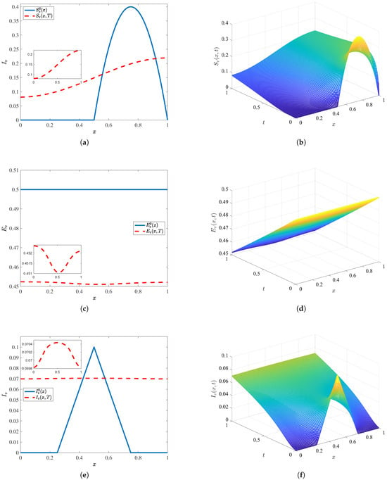
The numerical simulations are constructed with the following aims. In Example 1, the purpose is to simulate the constant-parameter reaction term with the previously considered parameters for the ordinary differential equation models. In the case of Example 2, the goal is the approximation of the numerical solution of the system (7)–(14) when some parameters are space-dependent functions. Meanwhile, in Example 3, the objective is to study the sensitivity of the solution to the diffusion coefficients.

5.2. Example 1

In this case, we consider the parameters defined in

Table 2. Parameters and coefficients used in the numerical examples. We remark that, in Example 3, the parameters used are those given in the column for Example 1 with the exception of $\mathbb{D}$.

Variable/Parameter	Example 1	Example 2
$\theta$	$0.020$	$0.02+0.01cos(3\pi x/2)$
$\Lambda$	$0.030$	$0.03+0.001cos(3\pi x/2)$
$\phi$	$0.090$	$0.09+0.01cos(3\pi x/2)$
$\psi$	$0.090$	$0.09+0.01cos(3\pi x/2)$
${\alpha }_c$	$0.010$	$0.010$
${\beta }_c$	$0.001$	$0.001$
$k_1$	$0.008$	$0.008$
$k_2$	$0.100$	$0.100$
${\mu }_v$	$0.010$	$0.010$
${\mu }_v^{*}$	$0.002$	$0.002$
$\mathbb{D}$	$\mathrm{diag}(0,0,0,0.1,0.1,0.1)$	$\mathrm{diag}(0,0,0,1,1,1)$

, $\mathsf{\Omega }=(0,1)$, $T=1$, $N=M=100$, and the initial condition for plant populations defined by the following relations:

$$\begin{array}{cccc}\hfill S_c^0\left(x\right)& =\left\{\begin{array}{cc}-(2/5)(4x-1)(4x-3)\hfill & x\in [1/4,3/4],\hfill \\ 0\hfill & \mathrm{otherwise},\hfill \end{array}\right.\hfill & \hfill & L_c^0\left(x\right)=0.2,\hfill \\ \hfill I_c^0\left(x\right)& =\left\{\begin{array}{cc}(4/5)x\hfill & x\in [0,1/4],\hfill \\ -(4/5)x+2/5\hfill & x\in [1/4,1/2],\hfill \\ 0\hfill & \mathrm{otherwise}.\hfill \end{array}\right.\hfill & \hfill \end{array}$$

Meanwhile, the initial conditions for vector populations are defined as follows:

$$\begin{array}{cccc}\hfill S_v^0\left(x\right)& =\left\{\begin{array}{cc}-(16/5)(2x-1)(x-1)\hfill & x\in [1/2,1],\hfill \\ 0\hfill & \mathrm{otherwise},\hfill \end{array}\right.\hfill & \hfill & E_v^0\left(x\right)=0.5,\hfill \\ \hfill I_v^0\left(x\right)& =\left\{\begin{array}{cc}(1/10)(4x-1)\hfill & x\in [1/4,1/2],\hfill \\ -(1/10)(4x-3)\hfill & x\in [1/2,3/4],\hfill \\ 0\hfill & \mathrm{otherwise}.\hfill \end{array}\right.\hfill & \hfill \end{array}$$

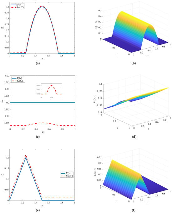
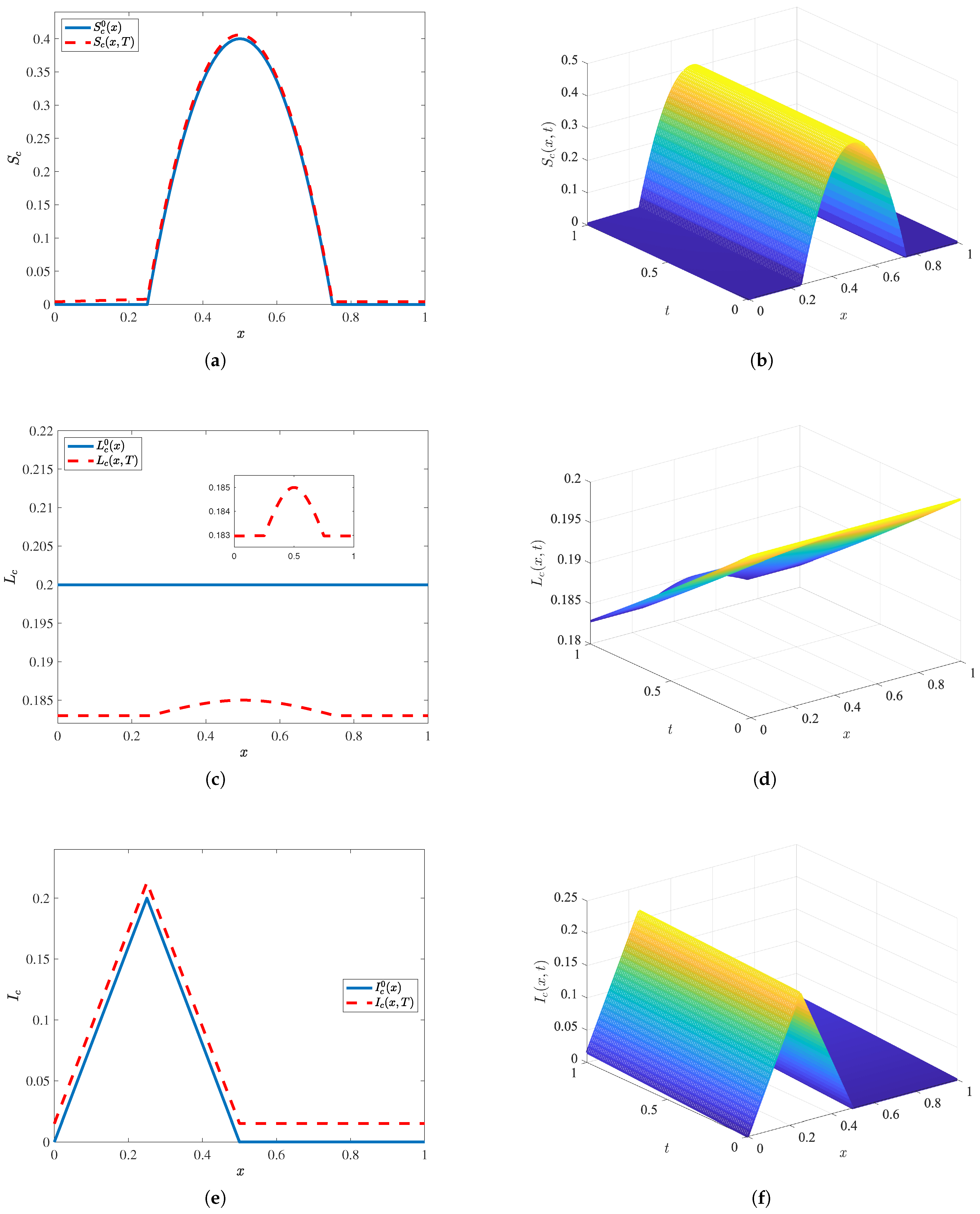
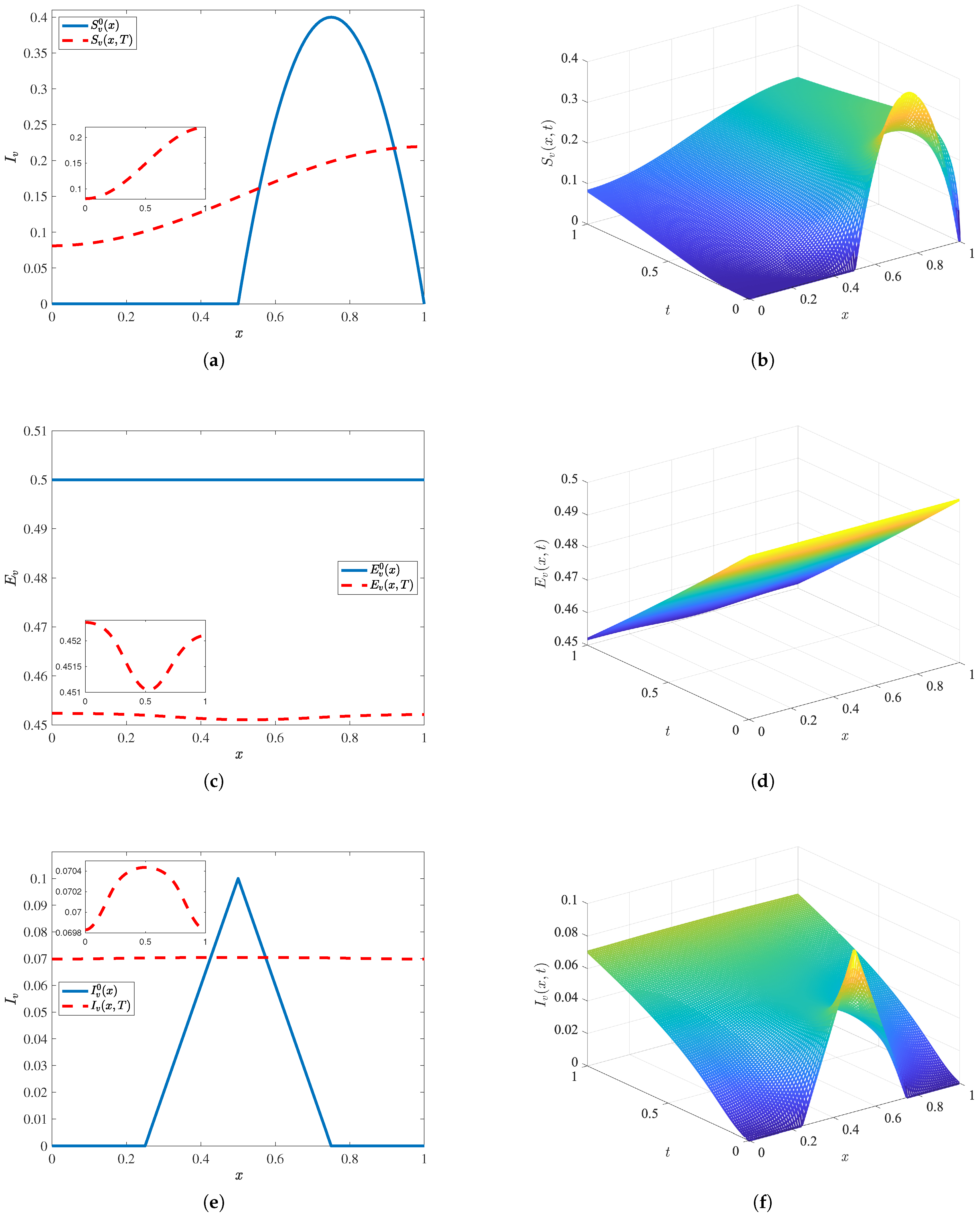
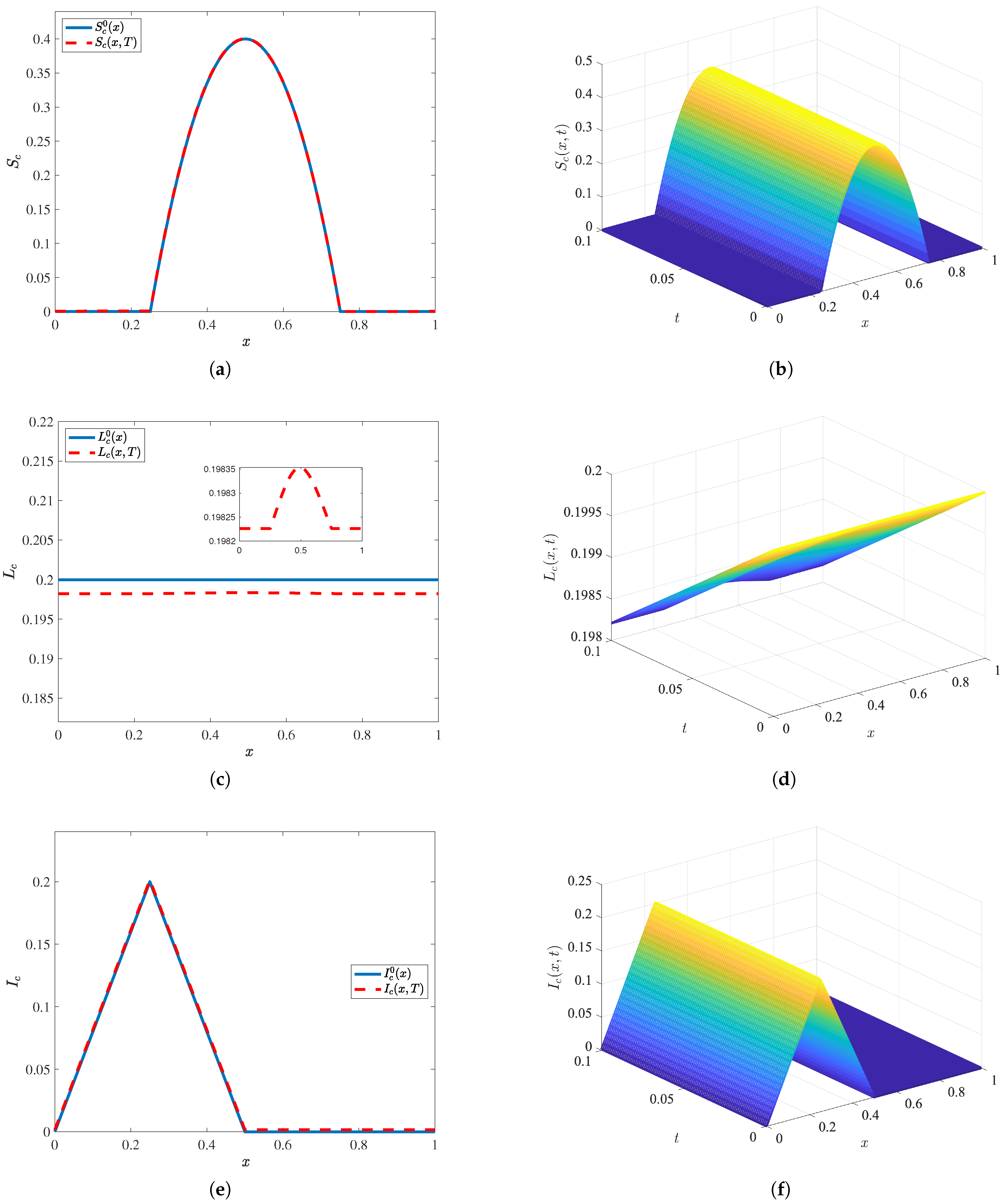
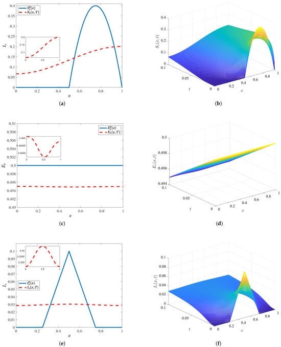
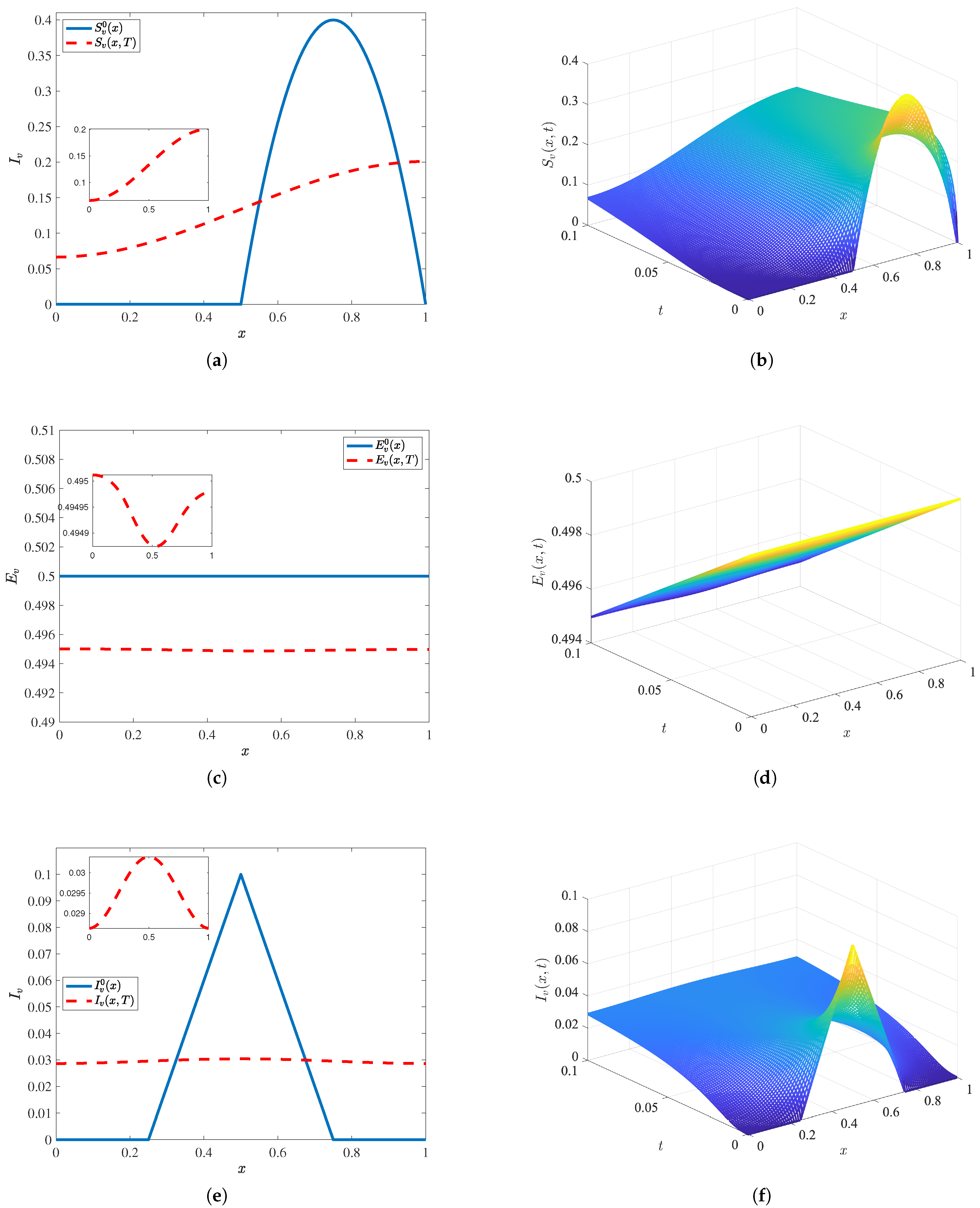
The results of the numerical solutions are presented in Figure 2 and Figure 3 for plant and vector populations, respectively.

We observe that the forms of plant populations preserve the geometric form of the initial condition, except for the latent plant population. This behavior occurs because the plants are fixed in space, or, equivalently, the diffusion vanishes for the entire plant population. Meanwhile, in the case of the vector population, influenced by the spatial displacement, we notice that the initial condition is regularized as time increases.

5.3. Example 2

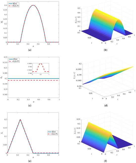
In this case, we consider the parameters defined in Table 2, $\mathsf{\Omega }=(0,1)$, $T=0.1$, $N=M=100$, and the initial condition given in Example 1. The results of the numerical solutions are presented in Figure 4 and Figure 5 for plant and vector populations, respectively. The aim of this example is to present a numerical solution with space-dependent coefficients. Particularly, we have considered periodic coefficients expecting to get a periodic solution profile. However, we have observed that the end profile solution is not periodic.

5.4. Example 3

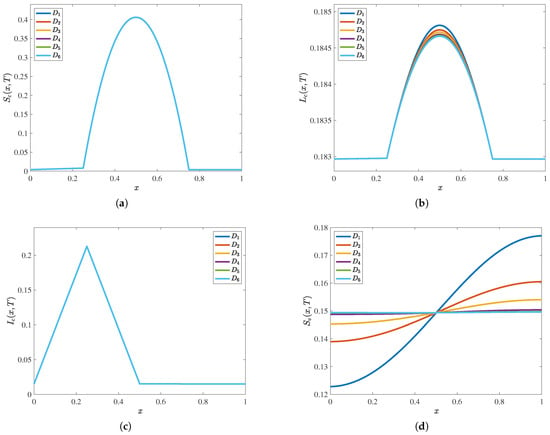
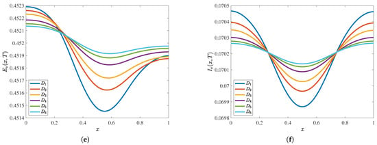
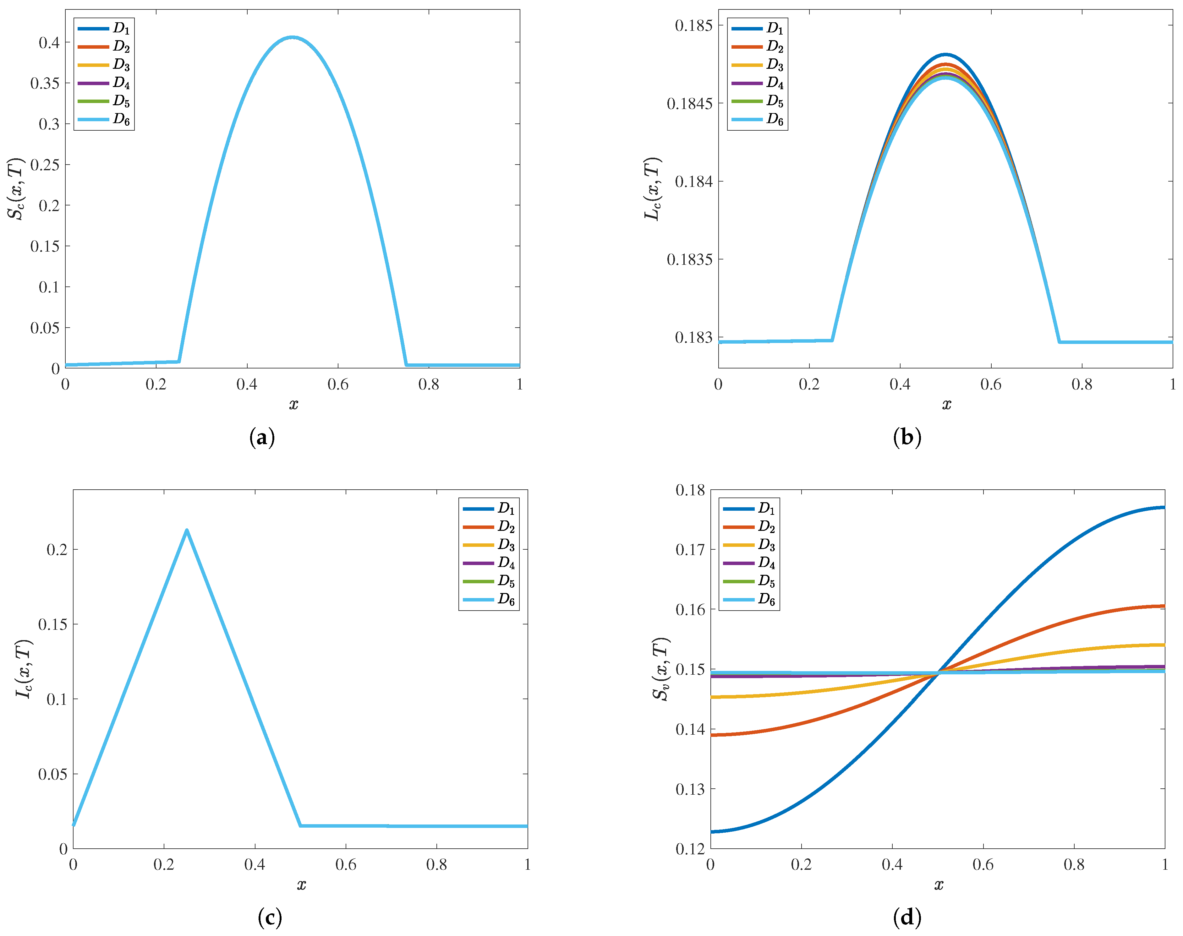
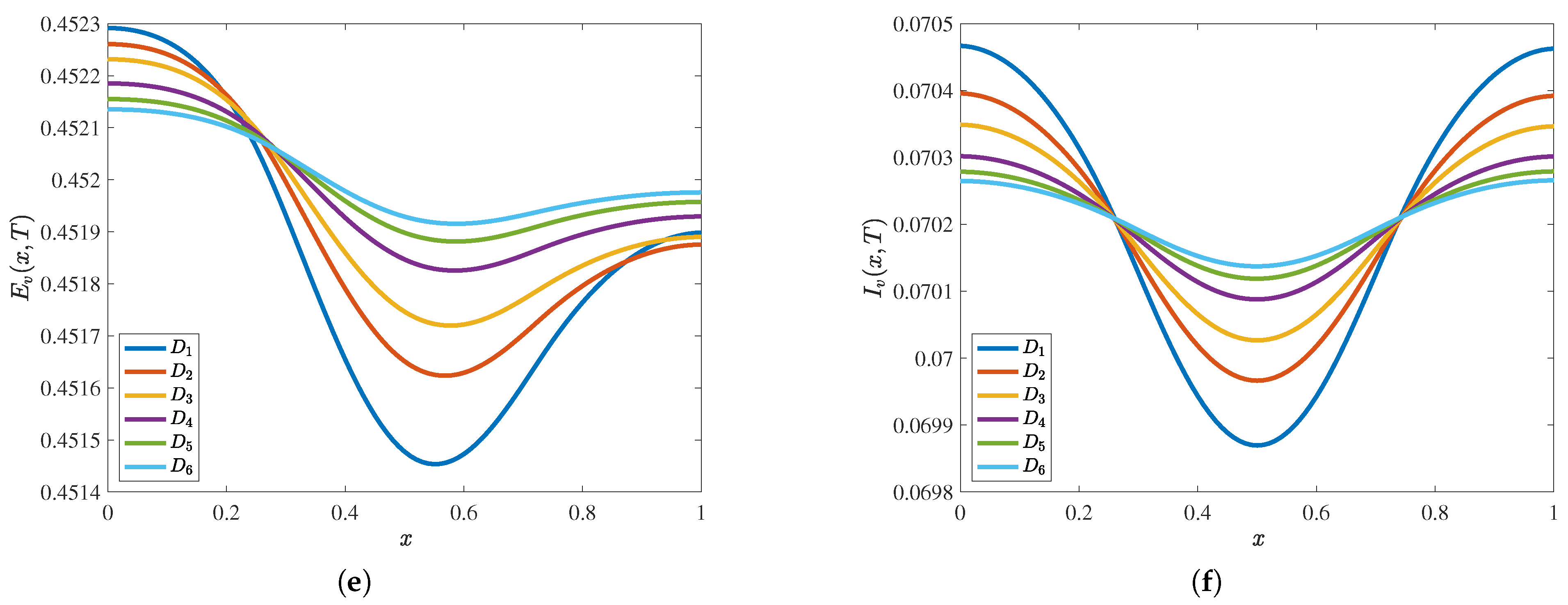
In this case, we consider the initial data, discretization parameters, and the biological parameters of Example 1. We develop six simulations with different diffusion parameters. More precisely, we consider the following diffusion coefficients:

$$\begin{array}{cccc}\hfill {\mathbb{D}}_1& =\mathrm{diag}(0,0,0,0.2,0.2,0.2),\hfill & \hfill {\mathbb{D}}_4& =\mathrm{diag}(0,0,0,0.6,0.6,0.6),\hfill \end{array}$$

(72)

$$\begin{array}{cccc}\hfill {\mathbb{D}}_2& =\mathrm{diag}(0,0,0,0.3,0.3,0.3),\hfill & \hfill {\mathbb{D}}_5& =\mathrm{diag}(0,0,0,0.8,0.8,0.8),\hfill \end{array}$$

(73)

$$\begin{array}{cccc}\hfill {\mathbb{D}}_3& =\mathrm{diag}(0,0,0,0.4,0.4,0.4),\hfill & \hfill {\mathbb{D}}_6& =\mathrm{diag}(0,0,0,1.0,1.0,1.0).\hfill \end{array}$$

(74)

The results of the numerical simulation are shown in Figure 6. We notice at least three types of behaviors influenced by the diffusion coefficient. First, susceptible and infected plant population profiles are not affected by the diffusion coefficients. Second, the latent plant population profiles have a monotonic behavior in the sense that, if ${\mathbb{D}}_i\le {\mathbb{D}}_j,$ then $L_c^{{\mathbb{D}}_i}(x,T)\ge L_c^{{\mathbb{D}}_j}(x,T)$ on $\mathsf{\Omega }$. Here ${\mathbb{D}}_i\le {\mathbb{D}}_j$ is understood as a partial order, i.e., in the component-wise sense, and $L_c^{{\mathbb{D}}_i}$ denotes the profile corresponding to ${\mathbb{D}}_i.$ Third, the susceptible, exposed and infected vector population profiles have a monotonic behavior on the boundaries. For instance, in the case of susceptible vector population profiles, we notice that, if ${\mathbb{D}}_i\le {\mathbb{D}}_j,$ then $S_v^{{\mathbb{D}}_i}(0,T)\le S_v^{{\mathbb{D}}_j}(0,T)$ and $S_v^{{\mathbb{D}}_i}(1,T)\ge S_v^{{\mathbb{D}}_j}(1,T)$.

6. Conclusions and Future Work

In this article, we have proposed a novel mathematical model for the dynamics of Huanglongbing disease, accounting for the spatial heterogeneity of two populations: citrus trees and psyllids. The model is formulated using the compartmental methodology and Fick’s law. The result is a coupled system of six equations: three ordinary differential equations and three reaction–diffusion equations. The ordinary differential equations model three sub-populations of citrus trees. Meanwhile, the reaction–diffusion unknowns model three psyllid sub-populations. This work demonstrates that the methodology of semigroup theory provides a rigorous framework for addressing the well-posedness of a nonlinear model describing the transmission dynamics of citrus greening disease under positive initial data and Neumann boundary conditions. The analytical findings reveal that sustaining citrus populations in the studied region requires the recruitment rate of susceptible plants to be no less than the infection pressure exerted by infected vectors. Moreover, controlling the spread of the disease is feasible when the force of infection from infected plants to vectors remains below the birth rate of susceptible vectors. These threshold conditions are critical for developing effective management strategies. The numerical simulations performed further validate and illustrate the theoretical results, providing insight into the practical implications of our model.

The modeling of disease transmission through partial differential equations has emerged as a rapidly evolving research domain over the past decade. Nonetheless, several unresolved questions remain, representing ongoing challenges and highlighting avenues for the refinement and extension of the present work. At a minimum, the following aspects merit further exploration:

• The inclusion of a natural predator for psyllid vectors, with minimal impact on citrus cultivation.
• The incorporation of time- and space-dependent coefficients for key model parameters, including the recruitment rate of citrus plants, the birth rate of vectors, and the infection pressures from both citrus and vector populations.
• A classical analysis of the proposed model, involving the computation of equilibrium points, the derivation of the basic reproduction number, and the subsequent assessment of equilibrium stability.
• The integration of a delay term into the model to account for the latency period of the pathogen within the psyllid vector, potentially enabling the prediction of future outbreaks.
• The exploration of parameter identification through an inverse problem approach. Moreover, an experimental validation of the proposed model, similar to the analysis developed in [70,71], must be considered as future work.

References

- Naciones Unidas. Objetivos de Desarrollo Sostenible. 2025. Available online: https://www.un.org/sustainabledevelopment/ (accessed on 30 April 2024).
- FAO. 2024. Available online: https://www.fao.org/home/en/ (accessed on 4 December 2025).
- Pratiksha; Adhikary, M. Industrial Production of Citrus By-products and Its Processing Techniques. In Citrus Fruits and Juice; Gupta, A.K., Kour, J., Mishra, P., Eds.; Springer: Singapore, 2024. [Google Scholar] [CrossRef] [Scilit]
- Lima, C.A.; Contato, A.G.; de Oliveira, F.; da Silva, S.S.; Hidalgo, V.B.; Irfan, M.; Gambarato, B.C.; Carvalho, A.K.F.; Bento, H.B.S. Trends in enzyme production from citrus by-products. Processes 2025, 13, 776. [Google Scholar] [CrossRef] [Scilit]
- FAO. Citrus I Markets and Trade. 2024. Available online: https://www.fao.org (accessed on 4 December 2025).
- USDA. Citrus: World Markets and Trade. 2024. Available online: https://www.fas.usda.gov (accessed on 4 December 2025).
- WCO. Facts and Figures. 2024. Available online: https://worldcitrusorganisation.org (accessed on 4 December 2025).
- Ghosh, D.; Kokane, S.; ySavita, B.K.; Kumar, P.; Sharma, A.K.; Ozcan, A.; Kokane, A.; Santra, S. Huanglongbing pandemic: Current challenges and emerging management strategies. Plants 2022, 12, 160. [Google Scholar] [CrossRef] [Scilit] [PubMed]
- Ferrara, T.F.d.S.; Schneider, V.K.; Kishi, L.T.; Carmona, A.K.; Alves, M.F.M.; Belasque-Junior, J.; Rosa, J.C.; Hunter, W.B.; Henrique-Silva, F.; Soares-Costa, A. Characterization of a recombinant cathepsin b-like cysteine peptidase from Diaphorina citri kuwayama (hemiptera: Liviidae): A putative target for control of citrus Huanglongbing. PLoS ONE 2015, 10, e0145132. [Google Scholar] [CrossRef] [Scilit]
- Ferrarezi, R.S.; Vincent, C.I.; Urbaneja, A.; Machado, M.A. Unravelling citrus Huanglongbing disease. Front. Plant Sci. 2020, 11, 609655. [Google Scholar] [CrossRef] [Scilit]
- COSAVE. Planes Regionales. 2017. Available online: http://www.cosave.org/pagina/planes-regionales (accessed on 4 December 2025).
- Servicio Agrícola y Ganadero. Huanglongbing de los Cítricos (HLB). 2019. Available online: https://www.sag.gob.cl/ambitos-de-accion/huanglongbing-de-los-citricos-hlb (accessed on 4 December 2025).
- Craig, A.P.; Cunniffe, N.J.; Parry, M.; Laranjeira, F.F.; Gilligan, C.A. Grower and regulator conflict in management of the citrus disease Huanglongbing in Brazil: A modelling study. J. Appl. Ecol. 2018, 55, 1956–1965. [Google Scholar] [CrossRef] [Scilit]
- Vilamiu, R.G.D.; Ternes, S.; Braga, G.A.; Laranjeira, F.F. A Model for Huanglongbing spread between citrus plants including delay times and human intervention. AIP Conf. Proc. 2012, 1479, 2315–2319. [Google Scholar]
- López-Collado, J.; López-Arroyo, J.I.; Robles-García, P.L.; Márquez-Santos, M. Geographic distribution of habitat, development, and population growth rates of the asian citrus psyllid, Diaphorina citri, in Mexico. J. Insect Sci. 2013, 13, 114. [Google Scholar] [CrossRef] [Scilit]
- Shimwela, M.M.; Schubert, T.S.; Albritton, M.; Halbert, S.E.; Jones, D.J.; Sun, X.; Roberts, P.D.; Singer, B.H.; Lee, W.S.; Jones, J.B.; et al. Regional spatial-temporal spread of citrus Huanglongbing is affected by Rain in Florida. Phytopathology 2018, 108, 1420–1428. [Google Scholar] [CrossRef] [Scilit] [PubMed]
- Garcia-Figuera, S.; Deniston-Sheets, H.; Grafton-Cardwell, E.; Babcock, B.; Lubell, M.; McRoberts, N. Perceived vulnerability and propensity to adopt best management practices for Huanglongbing disease of citrus in California. Phytopathology 2021, 111, 1758–1773. [Google Scholar] [CrossRef] [Scilit] [PubMed]
- Nguyen, V.A.; Bartels, D.W.; Gilligan, C.A. Modelling the spread and mitigation of an emerging vector-borne pathogen: Citrus greening in the US. PLoS Comput. Biol. 2023, 19, e1010156. [Google Scholar] [CrossRef] [Scilit]
- Ellis, J.; Lázaro, E.; Duarte, B.; Magalhaes, T.; Duarte, A.; Benhadi-Marín, J.; Pereira, J.A.; Vicent, A.; Parnell, S.; Cunniffe, N.J. Developing epidemiological preparedness for a plant disease invasion: Modelling citrus Huanglongbing in the European Union. Plants People Planet 2025, 7, 1403–1423. [Google Scholar] [CrossRef] [Scilit]
- Anguelov, R.; Lubuma, J.; Dumont, Y. Mathematical analysis of vector-borne diseases on plants. In 2012 IEEE 4th International Symposium on Plant Growth Modeling, Simulation, Visualization and Applications; IEEE: Piscataway, NJ, USA, 2012; pp. 22–29. [Google Scholar]
- Huancas, F.; Coronel, A.; Lozada, E.; Torres, J. Mathematical modeling of population dynamics of pollinators: A survey. Biology 2025, 14, 1308. [Google Scholar] [CrossRef] [Scilit]
- Bokil, V.A.; Allen, L.; Jeger, M.J.; Lenhart, S. Optimal control of a vectored plant disease model for a crop with continuous replanting. J. Biol. Dyn. 2019, 13, 325–353. [Google Scholar] [CrossRef] [Scilit]
- Coronel, A.; Huancas, F.; Lozada, E.; Rojas-Medar, M. The Dubovitskii and Milyutin methodology applied to an optimal control problem originating in an ecological system. Mathematics 2021, 9, 479. [Google Scholar] [CrossRef] [Scilit]
- Fitzgibbon, W.; Langlais, M.; Morgan, J. A mathematical model for indirectly transmitted diseases. Math. Biosci. 2007, 206, 233–248. [Google Scholar] [CrossRef] [Scilit] [PubMed]
- Coronel, A.; Huancas, F.; Berres, S. Study of an epidemiological model for plant virus diseases with periodic coefficients. Appl. Sci. 2023, 14, 399. [Google Scholar] [CrossRef] [Scilit]
- Taylor, R.A.; Mordecai, E.A.; Gilligan, C.A.; Rohr, J.R.; Johnson, L.R. Mathematical models are a powerful method to understand and control the spread of Huanglongbing. PeerJ 2016, 4, e2642. [Google Scholar] [CrossRef] [Scilit]
- Wang, H.; Cai, T.; Cao, W. Citrus Huanglongbing recognition algorithm based on CKMOPSO. Int. J. Cogn. Inform. Nat. Intell. 2021, 15, 1–11. [Google Scholar] [CrossRef] [Scilit]
- de Almeida, E.P.; Janeiro, V.; Guedes, T.A.; Mulati, F.; Carneiro, J.W.P.; Nunes, W.M.D. Modeling citrus Huanglongbing data using a zero-inflated negative binomial distribution. Acta Sci.–Agron. 2016, 38, 299–306. [Google Scholar] [CrossRef] [Scilit]
- Raiol, L.L., Jr.; Cifuentes-Arenas, J.C.; Cunniffe, N.J.; Turgeon, R.; Lopes, S.A. Modeling Candidatus Liberibacter asiaticus movement within citrus plants. Phytopathology 2021, 111, 1711–1719. [Google Scholar] [CrossRef] [Scilit]
- Luiz, M.H.R.; Takahashi, L.T.; Bassanezi, R.C. Optimal control in citrus diseases. Comput. Appl. Math. 2021, 40, 191. [Google Scholar] [CrossRef] [Scilit]
- Gao, S.J.; Yu, D.; Meng, X.Z.; Zhang, F.M. Global dynamics of a stage-structured Huanglongbing model with time delay. Chaos Solitons Fractals 2018, 117, 60–67. [Google Scholar] [CrossRef] [Scilit]
- Feng, J.L.; Wei, C.J. Initial size sensitivity in Huanglongbing dynamics: How branching processes challenge deterministic outbreak predictions. Appl. Math. Lett. 2025, 171, 109674. [Google Scholar] [CrossRef] [Scilit]
- Jacobsen, K.; Stupiansky, J.; Pilyugin, S.S. Mathematical modeling of citrus groves infected by Huanglongbing. Math. Biosci. Eng. 2013, 10, 705–728. [Google Scholar] [CrossRef] [Scilit] [PubMed]
- Djeffal, K.B.; Djilali, S.; Gul, N.; Ahmad, Z.; Saeed, T. Mathematical analysis of Huanglongbing transmission model in a periodic environment. Fractals–Complex Geom. Patterns Scaling Nat. Soc. 2023, 31, 2340080. [Google Scholar] [CrossRef] [Scilit]
- Wang, Y.; Gao, S.J.; Liu, Y.J.; Zhu, H.P. Modeling study of the effects of Ageratum Conyzoides on the transmission and control of citrus Huanglongbing. Plants 2023, 12, 3659. [Google Scholar] [CrossRef] [Scilit] [PubMed]
- Luo, L.; Gao, S.J.; Ge, Y.Q.; Luo, Y.Q. Transmission dynamics of a Huanglongbing model with cross protection. Adv. Differ. Equ. 2017, 2017, 355. [Google Scholar] [CrossRef] [Scilit]
- Liu, Y.J.; Gao, S.J.; Chen, D.; Liu, B. Modeling the transmission dynamics and optimal control strategy for Huanglongbing. Mathematics 2024, 12, 2648. [Google Scholar] [CrossRef] [Scilit]
- Luo, Y.Q.; Zhang, F.M.; Liu, Y.J.; Gao, S.J. Analysis and optimal control of a Huanglongbing mathematical model with resistant vector. Infect. Dis. Model. 2021, 6, 782–804. [Google Scholar] [CrossRef] [Scilit]
- Yan, S.X.; Huang, Z.R.; Gao, S.J.; Kang, Y. Dynamics of a citrus disease model with intercropping and insecticides: Application to Huanglongbing. Adv. Contin. Discret. Model. 2025, 2025, 98. [Google Scholar] [CrossRef] [Scilit]
- Anzo, A.; Hernández, C.A.; Giménez, U.J.; Oliveros, J.J. Optimizing control parameters for Huanglongbing disease in Citrus orchards using SAIR-SI compartmental model, epidemic final size, and genetic algorithms. J. Math. Biol. 2024, 90, 4. [Google Scholar] [CrossRef] [Scilit]
- Anzo-Hernández, A.; Giménez-Mujica, U.J.; Gracidas, C.A.H.; Oliveros-Oliveros, J.J. Investigating HLB control dtrategies using genetic algorithms: A two-orchard model approach with ACP Dispersal. Comput. Electron. Agric. 2025, 237, 110415. [Google Scholar] [CrossRef] [Scilit]
- Wang, J.P.; Gao, S.J.; Luo, Y.L.; Xie, D.H. Threshold dynamics of a Huanglongbing model with logistic growth in periodic environments. Abstr. Appl. Anal. 2014, 2014, 841367. [Google Scholar] [CrossRef] [Scilit]
- Tang, S.M.; Gao, S.J.; Zhang, F.M.; Liu, Y.J. Role of vector resistance and grafting infection in Huanglongbing control models. Infect. Dis. Model. 2023, 8, 491–513. [Google Scholar] [CrossRef] [Scilit] [PubMed]
- Zhang, F.M.; Qiu, Z.P.; Zhong, B.L.; Feng, T.; Huang, A.J. Modeling citrus Huanglongbing transmission within an orchard and its optimal control. Math. Biosci. Eng. 2020, 17, 2048–2069. [Google Scholar] [CrossRef] [Scilit]
- Lee, J.A.; Halbert, S.E.; Dawson, W.O.; Robertson, C.J.; Keesling, J.E.; Singer, B.H. Asymptomatic spread of Huanglongbing and implications for disease control. Proc. Natl. Acad. Sci. USA 2015, 112, 7605–7610. [Google Scholar] [CrossRef] [Scilit]
- Tu, Y.B.; Gao, S.J.; Liu, Y.J.; Chen, D.; Xu, Y. Transmission dynamics and optimal control of stage-structured HLB model. Math. Biosci. Eng. 2019, 16, 5180–5205. [Google Scholar] [CrossRef] [Scilit] [PubMed]
- Zhang, Y.W.; Deng, X.L.; Lan, Y.B. Reinforcement learning-based event-driven optimal prevention control strategy for citrus Huanglongbing model. Infect. Dis. Model. 2025, 10, 1334–1354. [Google Scholar] [CrossRef] [Scilit] [PubMed]
- Zhang, F.M.; Qiu, Z.P.; Huang, A.J.; Zhao, X. Optimal control and cost–effectiveness analysis of a Huanglongbing model with comprehensive interventions. Appl. Math. Model. 2021, 90, 719–741. [Google Scholar] [CrossRef] [Scilit]
- Chiyaka, C.; Singer, B.H.; Halbert, S.E.; Morris, J.G.; van Bruggen, A.H.C. Modeling Huanglongbing transmission within a citrus Tree. Proc. Natl. Acad. Sci. USA 2012, 109, 12213–12218. [Google Scholar] [CrossRef] [Scilit]
- Zhang, F.M.; Qiu, Z.P.; Feng, T.; Dai, Y.F.; Fan, G.H. Modeling the importation and local transmission of Huanglongbing disease: Bifurcation and sensitivity analysis. Int. J. Bifurc. Chaos 2022, 32, 2250117. [Google Scholar] [CrossRef] [Scilit]
- Zhang, F.M.; Qiu, Z.P.; Huang, A.J.; Cheng, Y.; Fan, G.H. Global dynamics and bifurcation analysis of an insect–borne plant disease model with two transmission routes. Int. J. Biomath. 2022, 15, 2250055. [Google Scholar] [CrossRef] [Scilit]
- Guo, J.; Gao, S.J.; Yan, S.X.; Liao, Z.Z. Bifurcation and optimal control analysis of delayed models for Huanglongbing. Int. J. Biomath. 2022, 15, 2250049. [Google Scholar] [CrossRef] [Scilit]
- Vilamiu, R.G.D.; Ternes, S.; Laranjeira, F.F.; Santos, T.T.D. Modelling the effect of an alternative host population on the spread of citrus Huanglongbing. AIP Conf. Proc. 2013, 1558, 2504–2508. [Google Scholar] [CrossRef] [Scilit]
- Liao, Z.Z.; Gao, S.J.; Yan, S.X.; Zhou, G.J. Transmission dynamics and optimal control of a Huanglongbing model with time delay. Math. Biosci. Eng. 2021, 18, 4162–4192. [Google Scholar] [CrossRef] [Scilit]
- Ternes, S.; Vilamiu, R.G.D.; Moreira, A.S.; Rossi, M.; Santos, T.T.D.; Laranjeira, F.F. Modelling citrus Huanglongbing spread in scenarios involving alternative hosts, vector populations and removal of symptomatic plants. J. Phytopathol. 2024, 172, e13445. [Google Scholar] [CrossRef] [Scilit]
- Liu, Y.J.; Gao, S.J.; Liao, Z.Z.; Chen, D. Dynamical behavior of a stage-structured Huanglongbing model with time delays and optimal control. Chaos Solitons Fractals 2022, 156, 111830. [Google Scholar] [CrossRef] [Scilit]
- Ling, W.W.; Wu, P.X.; Li, X.M.; Xie, L.J. Huanglongbing model under the control strategy of discontinuous removal of infected trees. Symmetry 2021, 13, 1164. [Google Scholar] [CrossRef] [Scilit]
- Xie, F.P.; Luo, Y.Q.; Zhang, Y.; Gao, S.J. High-dimensional modeling of Huanglongbing dynamics with time-varying impulsive control. Mathematics 2025, 13, 1546. [Google Scholar] [CrossRef] [Scilit]
- Xu, C.J.; Alhejaili, W.; Saifullah, S.; Khan, A.; Khan, J.; El-Shorbagy, M.A. Analysis of Huanglongbing disease model with a novel fractional piecewise approach. Chaos Solitons Fractals 2022, 161, 112316. [Google Scholar] [CrossRef] [Scilit]
- Liu, Y.; Gao, Y.R.; Zhang, F.M.; Gao, S.J. Dynamics of HLB transmission: Integrating saturated removal and vector bias in spatial/non-spatial models. Axioms 2025, 14, 434. [Google Scholar] [CrossRef] [Scilit]
- Souza, J.C.; Aparecido, S.; Cifuentes, J.C.; Fernandes, M.F.G. Flexible regression model for predicting the dissemination of candidatus Liberibacter Asiaticus under variable climatic conditions. Infect. Dis. Model. 2025, 10, 60–74. [Google Scholar] [CrossRef] [Scilit] [PubMed]
- Gao, S.J.; Guo, J.; Xu, Y.; Tu, Y.B.; Zhu, H.P. Modeling and dynamics of physiological and behavioral resistance of Asian citrus Psyllid. Math. Biosci. 2021, 340, 108674. [Google Scholar] [CrossRef] [Scilit]
- Kumar, P.; Ertürk, V.S.; Nisar, K.S. Fractional dynamics of Huanglongbing transmission within a citrus tree. Math. Methods Appl. Sci. 2021, 44, 11404–11424. [Google Scholar] [CrossRef] [Scilit]
- Li, Y.X.; Alshehri, M.G.; Algehyne, E.A.; Ali, A.; Khan, M.A.; Muhammad, T.; Islam, S. Fractional study of Huanglongbing model with singular and non-singular kernel. Chaos Solitons Fractals 2021, 148, 111037. [Google Scholar] [CrossRef] [Scilit]
- Martcheva, M. An Introduction to Mathematical Epidemiology; Springer: New York, NY, USA, 2015. [Google Scholar]
- Cantrell, R.S.; Cosner, C. Spatial Ecology via Reaction–Diffusion Equations; John Wiley & Sons: Hoboken, NJ, USA, 2004. [Google Scholar]
- Evans, L.C. Partial Differential Equations; American Mathematical Society: Providence, RI, USA, 2022; Volume 19. [Google Scholar]
- Sánchez-Garduño, F.; Breña-Medina, V. Searching for spatial patterns in a pollinator-plant-herbivore mathematical model. Bull. Math. Biol. 2011, 73, 1118–1153. [Google Scholar] [CrossRef] [Scilit]
- Tyson, R.C.; Wilson, J.B.; Lane, W.D. Beyond diffusion: Modelling local and long-distance dispersal for organisms exhibiting intensive and extensive search modes. Theor. Popul. Biol. 2012, 79, 70–81. [Google Scholar] [CrossRef] [Scilit] [PubMed]
- Yong, K.E. A Mathematical Model of the Interactions Between Pollinators and Their Effects on Pollination of Almonds. Ph.D. Thesis, The University of Iowa, Iowa City, IA, USA, 2012. [Google Scholar]
- Yong, K.E.; Li, Y.; Hendrix, S. Habitat choice of multiple pollinators in almond trees and its potential effect on pollen movement and productivity: A theoretical approach using the Shigesada-Kawasaki-Teramoto model. J. Theoret. Biol. 2012, 305, 103–109. [Google Scholar] [CrossRef] [Scilit]
- Wang, L.; Jiang, H.; Li, Y. Positive steady state solutions of a pant-pollinator model with diffusion. Discret. Contin. Dyn. Syst. Ser. B 2015, 20, 1805–1819. [Google Scholar] [CrossRef] [Scilit]
- Wang, J.; Yang, R.; Wang, J.; Cao, J. Threshold dynamics scenario of a plants-pollinators cooperative system with impulsive effect on a periodically evolving domain. Eur. J. Appl. Math. 2024, 35, 797–822. [Google Scholar] [CrossRef] [Scilit]
- Sánchez-Garduño, F.; Breña-Medina, V.E. Spatio-temporal dynamics of a three interacting species mathematical model inspired in physics. In Proceedings of the AIP Conference, Ponta Delgada, Portugal, 18–23 May 2008; Dagdug, L., Scherer, L.G.C., Eds.; Universidad Autonoma Metropolitana: Mexico City, Mexico, 2008; Volume 978, pp. 115–134. [Google Scholar]
- Krylov, N.V. Lectures on Elliptic and Parabolic Equations in Sobolev Spaces; American Mathematical Society: Providence, RI, USA, 2008; Volume 96. [Google Scholar]
- Adams, R.A.; Fournier, J.J. Sobolev Spaces; Volume 140 of Pure and Applied Mathematics; Elsevier/Academic Press: Amsterdam, The Netherlands, 2003; Volume 140. [Google Scholar]
- Pazy, A. Semigroups of Linear Operators and Applications to Partial Differential Equations; Springer Science & Business Media: New York, NY, USA, 2012; Volume 44. [Google Scholar]
- Barbu, V. Mathematical Methods in Optimization of Differential Systems; Springer Science & Business Media: London, UK, 2012; Volume 310. [Google Scholar]
- Carmo-Sousa, M.; Cortés, M.T.B.; Lopes, J.R.S. Understanding psyllid transmission of Candidatus Liberibacter as a basis for managing Huanglongbing. Trop. Plant Pathol. 2020, 45, 572–585. [Google Scholar] [CrossRef] [Scilit]
Disclaimer/Publisher’s Note: The statements, opinions and data contained in all publications are solely those of the individual author(s) and contributor(s) and not of MDPI and/or the editor(s). MDPI and/or the editor(s) disclaim responsibility for any injury to people or property resulting from any ideas, methods, instructions or products referred to in the content. |
© 2026 by the authors. Licensee MDPI, Basel, Switzerland. This article is an open access article distributed under the terms and conditions of the Creative Commons Attribution (CC BY) license.