


Abstract
We propose an agent-based, non-probabilistic framework for modeling the joint evolution of two discounted asset prices expressed in units of a third asset acting as numeraire. The framework is based on a trajectorial superhedging theory, in which pricing, arbitrage, and null events are defined purely in financial terms, without reference to probability measures or martingale assumptions. A central necessary theoretical requirement is that the global property -a.e. holds, ensuring consistency of the model construction. Admissible price evolutions are described by multidimensional trajectory sets generated from observable price movements and operational rebalancing rules representing a prescribed class of agents. Within a fixed trajectory set, relative price bounds between the two assets are obtained via superhedging and subhedging by means of self-financing portfolios that trade one asset against the other.
MSC:
60G07
1. Introduction
Classical asset pricing models rely on probabilistic assumptions that are rarely falsifiable and often difficult to justify empirically. In particular, joint models for multiple assets typically presuppose the existence of a stable probability law governing their co-movements, together with regularity assumptions that are imposed primarily for mathematical convenience. While such models are powerful, their practical use requires a substantial layer of calibration and statistical validation, and their conclusions are inevitably tied to the adequacy of the chosen probabilistic structure. For a critical view on the use of models in finance, see [1].
This paper adopts a different perspective. Rather than postulating an underlying probability measure, we work within a non-probabilistic, agent-based framework in which admissible price evolutions are described by trajectory sets constructed from observable market movements. The guiding principle is operational: trading decisions are triggered by price changes exceeding prescribed thresholds. Within this setting, pricing is formulated as a superhedging problem over a class of trajectories that encode historical price constraints and admissible rebalancing actions.
The present work focuses on the joint evolution of two discounted asset prices expressed in terms of a third asset acting as numeraire. The use of a two-dimensional trajectory construction is deliberate: it allows historical information about joint price movements to be incorporated directly into the admissible path structure. Superhedging prices, however, are computed using portfolios that trade only one of the assets against the other. This asymmetry is a methodology choice reflecting the distinction between information used to restrict admissible scenarios and our practical interest in obtaining model bounds for relative prices. In particular, the interaction between the two assets at the level of trajectory construction plays a crucial role in narrowing superhedging bounds compared to purely one-dimensional models. For a different agent-based approach, see [2].
The theoretical foundation of the approach builds on non-probabilistic superhedging operators and the treatment of arbitrage as a null-set phenomenon. Rather than excluding arbitrage paths a priori, the framework identifies them dynamically and suppresses their influence on prices through a notion of almost-everywhere validity adapted to the trajectorial setting. This perspective, developed in detail in earlier work, allows for a rigorous handling of pathwise arbitrage without invoking probability measures or martingale assumptions. The classical stochastic dictum of modeling market dynamics via (equivalent) martingale processes is here replaced by a global no-arbitrage-type constraint, namely the -a.e. property, where the notion of almost everywhere is defined purely in financial terms rather than probabilistic ones. This condition plays a structural role in the trajectorial framework by delimiting admissible model constructions and ensuring well-posed superhedging prices. Moreover, finer regularity properties familiar from martingale theory, such as upcrossing inequalities, can be used—together with empirical considerations—to further refine the space of modeling trajectories; this perspective is illustrated in Appendix D.
The modeling approach adopted in this paper is explicitly agent-based and operational. Rather than attempting to reproduce the full statistical structure of observed price series, we fix an operational protocol specifying the agent’s observation scale, triggering rules, and admissible actions, and study the superhedging implications within this constrained setting. Market data are used to populate feasibility regions induced by this protocol, not to calibrate a probabilistic law or to provide statistical validation across heterogeneous regimes. Accordingly, the numerical and empirical components of this paper are intended to illustrate feasibility and qualitative characteristics of the proposed models: they show how trajectory sets are constructed from historical observations, how pruning mechanisms affect admissible paths, and how resulting superhedging bounds respond to modeling choices. No claim is made that additional datasets, longer time horizons, or alternative calibration procedures would fundamentally alter the qualitative conclusions, as the emphasis is on exposing the mechanics of the method rather than optimizing empirical fit. This methodological perspective and its implications for data usage and calibration are discussed in detail in Section 7.1 and Section 7.2. Additional output and more exhaustive numerical experimentation are available in [3].
This paper demonstrates a principled, theory-based approach to non-probabilistic agent-based modeling of multi-asset markets that remains computationally explicit and operationally interpretable. Joint market information is encoded at the level of admissible trajectories, while pricing is carried out via trajectorial superhedging, yielding relative price bounds without probabilistic assumptions.
Relation to the Literature
The present work is situated within the growing body of non-probabilistic and robust approaches to mathematical finance, where pricing and hedging are formulated by relaxing the existence of an underlying probability measure. To gain perspective, our approach is located between the model-free arbitrage and superhedging theory in finite discrete time studied, e.g., by [4,5,6,7,8,9] and the pathwise superhedging approach to mathematical finance in continuous time initiated by Vovk [10] and further developed, e.g., in [11,12,13,14,15]. The infinite discrete-time framework also makes our approach closely related to the game-theoretic approach to probability of Shafer, Vovk, and co-authors, which is detailed in [16].
In contrast to classical (i.e., stochastic) arbitrage-free models, our setting admits trajectory sets for which there may not be a martingale measure (see Example 6 in [17]), while still allowing for well-defined superhedging prices. A detailed theoretical analysis of this phenomenon, including the role of null sets and conditional superhedging operators, is developed in [17] and related work. The closest stream of research to our approach is Game-Theoretical Probability, as fully described in [16]; we refer to [17] for a theoretical and detailed comparison. A key insight emerging from this line of research is that model consistency in our non-probabilistic setting is governed by a global almost-everywhere condition, rather than by pointwise exclusion of pathological scenarios. In particular, the -a.e. condition (see Section 3 in [17]) plays a role analogous to the existence of a martingale measure in classical asset pricing: it provides theoretical guidance for model construction by characterizing when a trajectorial market admits well-behaved superhedging prices, even in the presence of local arbitrage nodes. Crucially, the associated null sets are defined purely in financial terms and arise endogenously from the superhedging framework. As shown in [17], the -a.e. property admits verifiable sufficient conditions, making it a practical design criterion rather than a purely abstract assumption. Excluding arbitrage trajectories a priori is, in general, neither necessary nor desirable, as local removals may destroy the global structure required for superhedging to be well defined.
While robust and model-free developments ([18,19]) provide powerful pricing and duality principles, comparatively little work has used these theories as guidance for systematic, data-driven model construction. For loosely related references on superhedging, we point to [20,21,22]. A financial inspiration for our original ideas is reference [23]. The present paper follows the operational modeling philosophy developed in [24], in which trading decisions are triggered by observable market movements, and combines it with a trajectorial superhedging framework to construct multi-asset models. We describe how agent-based rebalancing rules, observable price excursions, and additional operational variables are used to generate and prune multidimensional trajectory sets, and how these modeling choices directly affect the resulting superhedging and subhedging bounds. The emphasis is on making explicit how modeling assumptions and market regimes enter the framework in a transparent and reproducible manner, rather than on statistical validation or the certification of optimal calibration. Our specific constructions should be viewed as one realization within a broader scenario-based superhedging framework, which remains flexible enough to accommodate alternative designs, including data-driven or learning-based approaches.
Admissible price evolutions are constructed in two dimensions, thereby encoding joint market information. On the other hand, superhedging valuation is deliberately restricted to one-dimensional trading so that relative prices reflect both the modeled co-movements of the assets and our intention to obtain model-based relative pricing bounds.
This paper is organized as follows: Section 2 introduces the trajectorial market setting and the basic modeling objects. Section 3 defines the operators used in our framework, including the almost-everywhere notion based on financially defined null sets. Section 4 indicates how our superhedging price bounds are evaluated as prescribed by our theoretical framework. Section 5 and Section 6 describe the operational, data-driven construction of two-dimensional admissible trajectory sets (encoding co-movements) together with pruning mechanisms. Section 7 shows our calibration procedure in specific historical data; geometric Brownian motion data is simulated to illustrate longer periods of data aggregation. Trajectory samples are also displayed. Section 8 describes output for a profit and loss analysis related to investments that are in between the subhedging and superhedging bonds. Section 9 ilustrates how arbitrage opportunities may appear during the trajectory set construction. Section 10 is an overview discussion of the modeling approach. Appendix A reports relevant material from [17] needed to support and justify our model constructions at different points. Appendix B details the superhedging algorithm in computational terms, how null sets are handled, and the computational complexity. Appendix C provides details of several prunning constraints. Appendix D presents an alternative, theory-based way to prune trajectories by what we call small arbitrage. The latter notion is illustrated by a Dubins type of upcrossing inequality.
2. Trajectorial Setting
We briefly introduce the mathematical setting underlying our models and refer the reader to Appendix A for theoretical developments and references (the original mathematical developments started in [25,26]). The framework models prices of a finite number of assets with known initial values, evolving in discrete trading stages. Conditioning on the information available at a given stage, uncertainty is represented by restricting future price evolutions to a prescribed set of multidimensional sequences, referred to as trajectories. These trajectories play the role of scenarios and encode admissible market evolutions directly, without reliance on probabilistic assumptions. Trading strategies are given by portfolios that are re-adjusted dynamically as information unfolds.
The framework is non-deterministic but non-probabilistic: admissible future prices are constrained by scenario sets rather than probability laws. One-dimensional versions of this approach appear in [27], while multidimensional extensions are developed in [28]. General one-dimensional superhedging theories allowing for infinitely many portfolios are studied in [17]. The present paper combines these strands: although we allow for an infinite family of portfolios to define null events, the resulting superhedging bounds coincide with those obtained from a single simple portfolio when required to hold almost everywhere in a non-probabilistic sense (Theorem A1).
The models presented in this paper provide concrete constructions of trajectory sets and thereby illustrate the general framework introduced below. We consider a financial market with assets evolving over a fixed time interval , with extensions to possible in much of the theory. For practical purposes, we will later specialize to the case . Trading occurs at discrete stages indexed by integers. Given initial prices , potential future prices are modeled by sequences
In what follows, we work with discounted prices, as explained next.
The trajectories we will construct are multidimensional and elements of a trajectory set denoted by . Elements are of the form , where , and the are d-tuples with coordinates that represent the prices of assets in units of asset . Additional coordinates in , indicated by …, will be described shortly. Specifically, the units are
where is one unit of asset and asset is the numeraire. Clearly, the choice of numeraire is arbitrary as long as the condition , is satisfied. In this paper, we refer to trajectories by ; this is in contrast to related work (e.g., [17]), where S is used. We are interested in modeling the former, i.e., the variables discounted by an arbitrary numeraire. To relate our work to the 1-dimensional trajectory sets introduced in the mentioned paper, we may think that we were taking and , representing one unit of a bank account (i.e., we deal with “discounted” prices).
Definition 1
(d-dimensional trajectory set). Consider a family of subsets of and a family of sets. For a given and , a trajectory set is a subset of
such that . Elements of are called trajectories.
The components are referred to as the traded coordinates, while the variables are called additional coordinates. In all applications of interest, is a strict subset of , reflecting modeling choices and market constraints. Designing suitable trajectory sets is a central goal of this paper. Apart from general no-arbitrage conditions introduced later (see Definition A3 and the notion of -a.e.), no restrictive assumptions are imposed on .
Portfolio rebalancing stages need not correspond to uniform time increments; this flexibility is handled through additional coordinates , which are used solely to construct and prune the trajectory set. These variables are not traded and play no role in the definition of superhedging operators or pricing once is fixed; when they are irrelevant, we suppress them and write trajectories simply as .
We provide an advance explanation of how the trajectory construction will operate. In the concrete constructions developed below, we set , where i labels successive –escapes (and hence portfolio rebalances), records the elapsed model time at the escape, and records the accumulated variation in the traded pair up to that stage. Precise definitions of –escapes, escape times, and variation are introduced later (Section 5.2 and Section 5.4). These quantities are modeling coordinates: they evolve along each candidate trajectory but are used exclusively to prune the recursively generated trajectory tree. Pruning is enforced through worst-case historical envelopes constructed from past windows, including one-argument bounds such as , which denotes the largest number of -escapes observed up to elapsed time across all historical windows, as well as bounds of the form , , and , together with other combinations such as and . In all cases, the corresponding lower bounds , , , , , and are imposed as well. In the implementation, the full family of such empirically derived one-argument constraints is exploited simultaneously in order to maximize pruning power and to restrict admissible scenarios to ranges supported by historical behavior.
While the choice provides a simple and relevant set of modeling coordinates, the framework readily accommodates additional or alternative coordinates when dictated by context or data availability. For example, transaction volume could be incorporated to regulate admissible rebalancing intensity—and hence the effective scope of arbitrage—by constraining trade sizes or frequencies, without affecting the pricing theory once the trajectory set has been fixed.
The index i labels rebalancing stages and need not correspond to the same physical time across different trajectories; the only requirement is that stage occurs after stage i along any given trajectory.
At stage k, the information available to investors is that the realized trajectory belongs to the conditional set
with . The pair is called a node and serves as shorthand for the conditioned trajectory set . As k increases, information accumulates and the sets become nested:
The multiplicity of trajectories emanating from a node captures the non-deterministic nature of future price evolution.
For later use, we define
where denotes the increment of the traded coordinates. Properties that depend only on will be called local.
Conditional Portfolio Sets
The second basic component of the framework is the class of admissible portfolios.
Definition 2
(conditional portfolio set). For any fixed and , denotes a set of sequences , where and are non-anticipative in the sense that whenever for . We assume is a vector space for each . Portfolios are required to be self-financing as in Definition 3.
Here, represents the number of units held of asset during the period , and we write for the Euclidean inner product in . The set need not contain all non-anticipative strategies. Elements of are called conditional portfolios.
It is also convenient to define global portfolios. For fixed , denotes the set of sequences such that, for every , there exists with for all and . Equivalently, a global portfolio restricts to a conditional portfolio on each node.
The value of the portfolio at stage i, expressed in units of the numeraire, is given by , while is its value just before rebalancing. To rule out external cash injections or withdrawals, we impose the self-financing condition.
Definition 3
(self-financing portfolio). A conditional portfolio H is called self-financing if for all and ,
Under the self-financing condition, portfolio gains and losses arise solely from increments of the traded coordinates. Accordingly, for and increments , the value of a portfolio with initial capital V and strategy H over the interval is given by
Note that V may depend on the realized node .
Finally, we introduce the elementary function spaces that form the basis for superhedging operators.
Definition 4
(elementary vector spaces). For a fixed node , define
Let denote the non-negative elements of . These sets are vector spaces since is assumed to be a vector space. Their elements are called elementary functions. We also define
3. Fundamental Operators and Almost-Everywhere Notion
Let Q denote the set of all functions from to , and let denote the set of all non-negative functions. Throughout, the following conventions are in effect: , , for all , and . A function is said to be of finite maturity if for some , which is then called the maturity time of f.
We introduce first an operator that will be used to define null objects and, in particular, the almost-everywhere notion in our framework. This operator plays the role of a conditional norm and will later be closely related to the superhedging operator.
Definition 5.
For a given node and , define
where for all .
The requirement that for all n with (as opposed to only at ) is only needed to treat certain arguments involving Type II nodes (see Appendix A.1). For brevity, we write .
For a general , define
Note that ; that is, is constant on the node . Moreover, , and hence . We refer to as a conditional norm.
We next introduce conditional notions of null sets and almost-everywhere properties.
Definition 6
(conditional a.e. notions). Given a node , a function is a conditionally null function at if
A subset is a conditionally null set at if . A property is said to hold conditionally almost everywhere at (equivalently, a.e. on ) if the subset of where it fails is a conditionally null set at . In particular, this definition applies to equalities of functions, written as a.e. on . The unconditional case corresponds to and is referred to simply as a.e. (or global null sets).
Definition 6 provides the notion of financial negligibility used later to justify removing Type II arbitrage nodes created during pruning without changing the reported superhedging/subhedging bounds.
All equalities and inequalities appearing below are understood to hold pointwise unless explicitly qualified by an a.e. statement.
We now introduce the central operator of this section.
Definition 7.
For a node and a general , define the conditional superhedging operator
where and, for , for all . Define also , and write . As before, depends only on .
The operator is the basic valuation functional applied later to the operationally constructed trajectory sets; it is the quantity computed numerically once the scenario graph and pruning constraints have been specified.
Null Sets as Unlikely Financial Events
We briefly explain the intuition behind the definition of the operator , with analogous considerations applying to . A simple superhedging portfolio for f is of the form for sufficiently large N. The idealization allowing a countable sum of non-negative portfolios serves a specific purpose: it enables the detection of arbitrage nodes (see Appendix A.1) and the definition of null sets.
This construction is directly analogous to Carathéodory’s approach to outer measures, where non-elementary sets are approximated by countable unions of elementary regions. Here, elementary regions are replaced by simple portfolios, which form a class closed under linear combinations and play the role of simple functions in classical integration theory (see Section 2.3 of [17]). Accordingly, can be interpreted as a conditional outer integral, obtained by restricting attention to the future paths in . Related perspectives appear in [29].
The presence of a single portfolio with arbitrary sign in Definition 7 is essential. By contrast, the idealized portfolios with are introduced solely to identify null functions. Indeed, the definition of nullity is intrinsically financial: a payoff f is null if, for every , there exists a family of non-negative portfolios such that while .
For instance, let with and . Then, f is null if it can be superhedged at arbitrarily small cost, despite offering a potentially unbounded payoff relative to the initial investment. This situation is analogous to a lottery ticket purchased at negligible cost but offering a large possible reward. Events of this type are therefore deemed financially negligible and are treated as null sets in the theory.
Arbitrage opportunities provide a canonical example. Suppose have unfolded and that for some and for all . Such a future constitutes an arbitrage opportunity via trading between the numeraire and the asset. One can then construct arbitrage portfolios that are activated on and satisfy for all . This allows one to take , showing that is a null function.
The need for a countable family arises because individual gains of the form may be arbitrarily small. Allowing countable collections of positive portfolios aligns the theory with modern integration, in particular with the ability to handle countable unions of null sets (see [17]).
4. Computational Formulation of Superhedging Prices
As discussed above, the use of a countable family of portfolios in the definition of is essential for handling countable collections of null sets, in direct analogy with Lebesgue’s theory of integration. Theorem 1 below shows that, when computing superhedging prices for finite-maturity payoffs, this idealization can be eliminated at the level of computation: the infinite sum of elementary portfolios can be replaced by a single elementary portfolio, provided the superhedging inequality is interpreted in an almost-everywhere sense.
More precisely, for functions depending on finitely many coordinates, superhedging can be achieved by a single simple portfolio yielding the same price bounds, with the understanding that violations may occur on null sets. In this way, the idealization of countably many portfolios enters only through the definition of null events. This mirrors the classical measure-based theory; see [29] for an analogous result.
An important consequence is that arbitrage nodes can be incorporated naturally into the model without affecting price bounds. Since arbitrage nodes give rise to null sets, specifically to trajectories belonging to the set (see (A2)), they can be neglected when computing superhedging prices. This principle is used repeatedly in our trajectory construction process, which may introduce arbitrage opportunities as a side effect of the pruning phase; such nodes are automatically neutralized at the pricing stage.
Theorem 1 below is essentially Theorem 6.1 of [17]. Appendix A provides the background needed to interpret the statement; in particular, that appendix presents and proves Theorem A1, a slight reformulation of Theorem 1 that is more convenient for our purposes. The precise meaning of the key hypothesis -a.e. is given in Appendix A, and sufficient conditions for its validity are discussed in [17].
For simplicity, the result is stated globally (i.e., at node ) and in the one-dimensional case. The theorem appears in [17]; while the converse statement is also established there, it will not be needed in the present work.
Theorem 1.
Suppose that -a.e. holds, that , and that is bounded and has finite maturity , that is, for all . Then,
Although our models describe the joint time evolution of the traded coordinates , that is, a -dimensional setting, the superhedging problems considered below involve one-dimensional portfolios. Specifically, we determine trading strategies in asset at prices in order to superhedge at a prescribed future time (of course, roles could be reversed).
The numeraire component of the portfolio, corresponding to holdings in a third asset , need not be included explicitly in the computation. Once the algorithm determines the trading positions in , the corresponding numeraire holdings are obtained directly from the self-financing condition (2). From a computational viewpoint, this amounts to extracting one-dimensional trajectories from the two-dimensional trajectories .
The relation between arbitrage properties in the two- and one-dimensional settings is as follows (node types are defined in Appendix A.1). A two-dimensional arbitrage-free node is also arbitrage-free when restricted to either coordinate or . Conversely, a two-dimensional arbitrage node need not induce a one-dimensional arbitrage opportunity. Intuitively, certain arbitrage opportunities only become accessible when simultaneous trading in both assets is permitted.
As a consequence, when computing superhedging prices using one-dimensional portfolios, the extracted one-dimensional trajectories may pass through nodes that are arbitrage nodes in the one-dimensional sense (Type II nodes; see Appendix A, Appendix A.1). However, as shown in [17], trajectories passing through such nodes form a null set. Since null sets do not affect superhedging prices, these nodes can be safely neglected in the computation.
This interplay between the two-dimensional trajectory construction and the one-dimensional pricing procedure is formalized in Appendix A, where we also present the dynamic programming algorithm used to compute superhedging prices and explain explicitly how arbitrage nodes are handled computationally.
5. Operational Definitions and Empirical Increment Set
As indicated, the theoretical framework developed in Section 2, Section 3 and Section 4 dictates null events and the superhedging operations, in particular through the almost-everywhere notion used for superhedging. The global necessary requirement for the theory to work is the -a.e. property that is needed in Theorem 1 and introduced in Definition A4 in Appendix A. In contrast, the generation of admissible scenarios is a modeling task, and arbitrage nodes may arise during trajectory construction and are not removed a priori, as doing so could alter drastically the global structure of the resulting trajectory set. Instead, their role is handled at the valuation stage, where the theory ensures that such nodes can be ignored when computing superhedging prices under the appropriate a.e. conditions (as per Theorem 1).
We work in the following financial context: we model the future joint evolution of discounted prices, expressed in units of a third asset acting as numeraire [30], for two traded assets (stocks). The central question addressed by our models is as follows: how much capital is required to superhedge one asset using the other? More precisely, the framework allows us to evaluate a relative superhedging amount, namely the investment needed to construct a self-financing portfolio that trades in one stock and the numeraire in order to superhedge the value (in numeraire units) of one share of the remaining stock. The symmetry of the methodology allows the roles of the two assets to be exchanged, as well as for subhedging or alternative choices of numeraire.
A natural data structure for representing the resulting trajectory sets is a directed graph. The construction proceeds locally at each node through two conceptually distinct stages. First, a collection of candidate child nodes is proposed so as to ensure that is arbitrage-free. Second, some of these proposed child nodes may be pruned, that is, removed if they violate prescribed constraints. While the proposal stage enforces local no-arbitrage, the pruning stage operates independently and may reintroduce arbitrage nodes. This phenomenon can arise naturally in the algorithmic construction, particularly when pruning constraints are calibrated with the intention of allowing greater risk in exchange for potential gains.
The separation between the proposal stage and the pruning stage is deliberate. The proposal stage delivers the absence of immediate two-dimensional arbitrage as well as a variety of possible trajectory unfoldings. On the other hand, the pruning stage operates independently and may therefore reintroduce arbitrage nodes. This independence reflects the fact that pruning constraints are modeling choices, introduced to restrict admissible scenarios based on operational or empirical criteria, and are not designed to preserve local no-arbitrage properties.
When pruning gives rise to arbitrage nodes of Type II in the one-dimensional projection used for pricing, the superhedging operators developed in Section 3 and Theorem 1 in Section 4 provide a justification for neglecting such branches as the trajectories passing through Type II nodes form a null set for the corresponding one-dimensional superhedging problem and therefore do not affect the computed price bounds.
5.1. Operational Data Processing
We introduce the framework used to implement an operational approach in the construction of trajectory market models. All variables are treated in discrete form. Accordingly, with a slight abuse of notation, an interval is understood as
where time is observed with smallest resolution (typically measured in minutes), reflecting the fact that an investor can only observe and act on the market at such increments.
Historical times are taken to be negative, with 0 denoting the present and positive times corresponding to the future. We denote by
the full observable historical time set, representing the entire past available to the agent.
Within , we partition the historical timeline into non-overlapping time windows of fixed length . The parameter T represents a local time horizon and should not be confused with the total observable history . We write
where denotes the number of discrete observation times contained in a single window, and define
In the present trading context, a window of length T typically corresponds to a full trading day, although the construction applies to arbitrary fixed horizons. The same fixed length T is also used as the window size for processing historical data along . We often write , with , and refer to as a time interval or time window. The collection of all such disjoint intervals is denoted by
Let denote undiscounted market prices at time , where plays the role of numeraire. Discounted prices (or charts) are obtained by normalization,
and we write . Entire charts are denoted by and . The chart is constant and is not explicitly included in the construction. Both undiscounted and discounted charts are assumed to move in discrete increments, but for different reasons. Undiscounted prices naturally admit a smallest unit, given by the currency in which they are quoted. By contrast, discounted charts arise as ratios of prices and therefore do not possess an intrinsic minimal unit of change: in principle, they may take arbitrary rational values. In practice, the investor observes historical data and determines discretization parameters operationally, based on observed price movements and modeling requirements. This choice is therefore part of the modeling procedure rather than a feature imposed by the market.
5.2. -Escapes and -Escape Times
This subsection specifies how a trading agent rebalances their portfolio in response to observable changes in chart values. We refer to this setup as operational to emphasize that portfolio rebalancing is triggered by quantities that are directly observable in the market. This link between observed chart evolution and model trajectories is the central mechanism driving the construction of our models, and, as argued in [24], it provides an objective basis for associating empirical data with admissible future scenarios. While many alternative operational prescriptions are possible, the definitions below are chosen to highlight features that are robust and adaptable to other settings.
The construction is motivated by well-known regularity properties of martingales, which play a fundamental role in financial modeling through the first fundamental theorem of asset pricing [31]. Classical results such as Doob’s and Dubins’ upcrossing inequalities [32,33], as well as Burkholder’s bounds on the number of escapes [34], describe how martingale paths fluctuate over time. More recent work on non-probabilistic martingales, closely related to no-arbitrage considerations (see [16,17]), shows that such regularity phenomena do not rely on probability and therefore have broader applicability. These observations serve as motivation for the operational notions introduced next.
-escapes and -escape times are defined for two alternative models, denoted A and B. In both cases, the definitions are understood relative to a fixed chart x and a fixed time window .
Definition 8
(Model A). For given parameter values and , define the δ-escapes
For , define the i-th δ-escape time recursively by
whenever the set on the right-hand side is nonempty; otherwise, is left undefined.
Definition 9
(Model B). For a given parameter value and , define the δ-escape
For , define the i-th δ-escape time recursively by
whenever the set on the right-hand side is nonempty; otherwise, is left undefined. For , set .
For either model, we say that the i-th -escape has occurred if is defined, and we let N denote the largest integer i such that is defined (with if is undefined). The sequence is called the sequence of -escape times, and N is the number of -escapes occurring within the interval . We note that is always included, and . For future reference, we write and use the notation .
Escape times are defined on a fixed observation grid of resolution and are triggered when a prescribed spatial threshold is exceeded in either traded coordinate. Because escape times are first hitting times on a -grid, the increment recorded at an escape may overshoot the threshold by at most one observation step. If one assumes (or empirically verifies) a bound on one-step relative movements at scale , then -escape increments are uniformly bounded by “threshold + one-step modulus.” Equivalently, imposing a uniform modulus of continuity on each individual chart at scale ensures that the empirical increment set remains bounded. Under aggregation at fixed , longer datasets or crisis windows increase escape frequency and modify pruning envelopes but do not introduce unbounded increment directions; qualitative changes arise only if the operational scale itself is altered. Details are presented in Section 7.1 and Section 7.2.
5.3. Discretization
While the notation is initially used to represent exact asset values, discretized variables are required for the construction of trajectory sets. For , let denote the discretization parameter associated with the discounted chart . We write for rounding to the nearest integer and for rounding to the nearest integer multiple of . Accordingly, we define integers by
Unlike undiscounted prices, discounted charts do not possess a natural minimal unit of change, as they arise from ratios of prices. The choice of discretization parameters is therefore not intrinsic to the market but is made operationally by the investor, based on observed historical data and modeling considerations. Depending on this choice, the discretized values may or may not coincide exactly with observed historical values. The integers should thus be interpreted as encoding discretized movements rather than exact prices.
To emphasize the discrete-time nature of the construction, we occasionally index these quantities by time increments. Writing with , we introduce integers such that
When historical data admit a smallest discrete unit, as is the case for prices quoted in currency units, the above discretization can be chosen to be exact.
5.4. Variation
We introduce next the notion of accumulated variation (or simply variation) as a convenient summary of historical chart movements. This quantity corresponds to one of the additional coordinates introduced abstractly in Definition 1. Its primary role is operational: variation provides an empirically measurable control variable that can be used to restrict future scenarios through pruning constraints.
Fix a time window , and let with , . At each such time, the discretized asset values are given by for (equivalently, ). Using these quantities, the accumulated variation is defined by
Thus, aggregates the combined integer movements of both charts over the interval . It is integer-valued, non-negative, and unitless, and does not depend explicitly on any discretization parameter. While our primary interest lies in modeling future asset values, accumulated variation is introduced mainly as a pruning device: by conditioning on historically observed values of , we can impose worst-case constraints on admissible future trajectories (see Section 6.1 and Appendix C). Other choices of variation, such as discrete analogs of quadratic variation, could also be employed; in later sections and appendices, we introduce variants derived from (5) when needed.
5.5. The Empirical Set
A key definition in our model construction is the empirical set introduced below. It represents the collection of relevant (to the investor) joint observable price increments occurring at all -escape times and aggregated over all historical time windows. The role of is to encode, in discretized form, the empirical joint movements that will be used as admissible building blocks for future trajectories.
We construct the set of empirical changes for a fixed time window as follows. Moving along the interval , we recursively build the -escape times according to Definition 8 (Model A) or Definition 9 (Model B). At each -escape time, we collect vectors
which represent variable increments between consecutive -escape times.
More precisely, for and for each of the two models, the following increments are defined:
where in the last line, and for some , . If , then all of the above variable increments are set to 0. Notice that , , and are integers (with and non-negative), and that the variation has no discretization parameter and is therefore unitless.
Hence, the set of chart changes over the window is defined as the collection of all such vectors, rounded to their nearest discretization parameters:
where the notation was introduced at the end of Section 5.2 and . The third coordinate reflects the identity . When , the cardinality of satisfies , while if , the set consists of the single vector .
The set of empirically measured chart changes is obtained by collecting these vectors over all historical time windows. For clarity, we define
where I was introduced in Section 5.1. The size of is given by . Figure 1 illustrates a typical instance of the convex hull generated by the first two coordinates of under Model B.
Figure 1.
First two components of the set constructed under Model B from historical data ().
Empirically, the vertices of the convex hull generated by the first two components of appear to be the ones that influence the value of in the present setting. When this behavior holds, it can be exploited to compute price bounds efficiently using the backward dynamic programming algorithm described in Appendix B.
Figure 1 displays the dimensionless integer pairs obtained from the construction of under Model B. The black lines represent the convex hull of the observed set, and the highlighted points correspond to its vertices.
6. Construction of Trajectory Set : Recursion and Pruning Constraints
This section makes explicit the trajectory sets generated under Models A and B. Elements of are called model trajectories and are constructed recursively using historical values of observed charts. Models A and B differ only in the definition of -escape times and the resulting consequences (such as the set , from Section 5.5, and the associated pruning constraints); apart from these distinctions, the trajectory-generation procedure is identical in both cases. The purpose here is to assemble these components into a concrete, recursive description of admissible trajectories, which will serve as the fixed scenario space for the superhedging and valuation procedures developed in subsequent sections.
A trajectory set consists of trajectories , that is, sequences of multidimensional vectors , where is referred to as a node. A trajectory may equivalently be viewed as a collection of nodes connected by directed edges. Empirical historical chart counterparts are denoted using lowercase letters, namely and . The variables and represent model asset values, represents the model time at the -escape, and represents the accumulated variation in the two-dimensional vector at the same escape.
These associations between model and historical quantities imply that trajectories take values on a discrete grid determined by the historical time parameter and the investor-calibrated parameters and . In particular,
The empirical parameter N, introduced after Definitions 8 and 9, is represented in the model by an integer . Trajectories terminate after a finite number of steps, that is, . The last (potential) trade occurs at index along the model trajectory , and the model coordinate does not necessarily coincide with the terminal time T.
We begin with the initial state , where , , and , are the most recent discounted chart values. Given an empirical set , corresponding to a specific choice of Model A or B, trajectories are generated recursively with respect to the index i, which we refer to informally as time steps. More precisely, the index i represents the (potential) portfolio rebalance along the trajectory. Thus, trajectory values are not constructed at all possible times, but only at specific times associated with historical -escapes, which trigger portfolio rebalances. Along a given trajectory, and record the model time and accumulated variation at the rebalance, while i counts the number of rebalances that have occurred so far.
Given a node with , trajectories are constructed iteratively as follows. For each (introduced in Section 5.5), define a successor node by
This procedure is continued recursively. At each step, the set is added to the most recent node of each trajectory, so that the number of trajectories grows exponentially, with at most trajectories available at step i. Figure 2 illustrates this construction for the first two coordinates.
Figure 2.
Generation of candidate successor nodes from a given state under the extension step ().
Figure 2 illustrates the extension step prior to pruning. The black point represents the current node . Blue points denote candidate successors obtained by adding all empirical increments to . The red polygon corresponds to the convex hull of these candidate successors. Admissibility of successors is enforced separately through the pruning constraints.
6.1. Pruning Constraints
In order to limit the growth of the trajectory set and, more importantly, to ensure that admissible trajectories reflect observed historical behavior, we introduce pruning constraints, also referred to as pruning functions. These constraints are determined by the additional modeling variables introduced earlier (see Definition 1) and constitute an essential component of the trajectory construction. An appropriate selection of such variables leads to constraints that are both tight—yielding narrow superhedging bounds—and stable under aggregation of historical data. Moreover, the variables entering the pruning constraints should complement one another, with each capturing different aspects of market behavior.
The purpose of the pruning functions is to restrict the admissible future evolution of the model variables to ranges supported by historical observations. We adopt a worst-case methodology: trajectories corresponding to scenarios that have not appeared in the historical record are excluded. Appendix D presents an alternative, theory-driven approach to pruning that is conceptually distinct from the data-based constraints considered here.
Each pruning constraint consists of a pair of functions, a maximum and a minimum, denoted by * and *, respectively. These functions are constructed from a given chart x and all historical windows . A third argument specifies the modeling variable to which the constraint applies; this may be time , the number of -escapes i, or the accumulated variation w. The precise form of the constraints depends on the choice of model (A or B), through their reliance on rebalancing times, although this dependence is left implicit in the notation.
We now provide a representative example of a pruning constraint/function; additional constraints are presented in Appendix C. All these pruning functions are used simultaneously in order to fully specify a model.
Definition 10
(historical maximum and minimum number of -movements at time ). For a given chart x, time interval , portfolio rebalancing times , and , define the number of δ-movements in the interval by
The corresponding historical maximum and minimum numbers of δ-movements at time ρ are then defined as
for .
When constructing future model trajectories, a proposed trajectory segment with time coordinate is discarded if the constraint
is violated. The effect of such pruning constraints on the trajectory set is illustrated in Figure 3, while Figure 4 displays the corresponding historical minimum and maximum numbers of rebalances.
Figure 3.
Dynamic pruning during trajectory construction up to depth .
Figure 4.
Historical bounds on the number of -escapes used as pruning constraints (Model B, ).
Figure 3 illustrates the pruning mechanism applied after candidate successors are generated from empirical increments in . Nodes correspond to partial trajectories . From each node, candidate successors are first constructed through the extension step. Pruning constraints are then enforced: red branches violate at least one constraint and are discarded, while blue branches remain admissible and are retained in the trajectory set.
Figure 4 displays the historical minimum and maximum numbers of -escapes observed up to time across all historical windows, thereby defining admissible ranges for the rebalance index i at a given model time. During trajectory construction, candidate nodes that violate these bounds are discarded. The parameters used in this example are and with . The apparent monotonicity is empirical and not imposed by the model.
6.2. Dynamic Pruning
Once all candidate successor nodes have been generated from a given node using the set , we determine whether these future states are historically realistic by enforcing the pruning constraints introduced in Section 6.1 and Appendix C. Nodes satisfying these constraints are said to be admissible. For future reference, we denote by the set of admissible nodes constructed recursively from , namely
To evaluate admissibility, we rely on the notation , , , , , , , , , , , , , and , which denote the evaluation of the corresponding maximum and minimum pruning constraints, introduced in Appendix C, at the node . For simplicity, we suppress the arguments x and I used in Appendix C. In contrast with the definitions given there (see also Section 6.1), constraints are evaluated here only at the generated times and, when applicable, only at the generated variations .
Hence, a node
is admissible if it satisfies the following pruning constraints:
We say that dynamic pruning is in effect when these constraints are enforced during the construction of the trajectory set.
The trajectory set is constructed by an operational, data-driven procedure based on the empirical set and the pruning constraints. The theory enters at the pricing stage: in relative pricing, we trade only one coordinate (say , together with the numeraire), so the key requirement is that property -a.e. holds for the induced one-dimensional model used for superhedging, rather than for the full multidimensional trajectory space. The superhedging computation is carried out via a dynamic programming algorithm (see Appendix A). The co-moving coordinate plays the role of a pathwise multivalued payoff function (i.e., a relation) of . When the additional state variables are reinstated, this relation becomes single-valued along each trajectory, while these variables are suppressed in the one-dimensional pricing recursion.
The two-dimensional construction encodes co-movement information directly into the admissible scenario set. By building and pruning trajectories in the joint variables (together with their associated state coordinates), the model constrains admissible joint price evolutions prior to pricing. This modeling choice is expected to lead to tighter superhedging and subhedging bounds than a purely one-dimensional construction, since co-movement information has already been enforced at the level of admissible scenarios.
The construction of admissible trajectories raises the question of how well such trajectories align with historically observed price paths that are not used in model building. This issue, commonly referred to as trajectory matching, is governed by the choice of the extension set introduced in Section 5.5, which specifies how trajectories are continued one step forward. In the present paper, is constructed from the data used in model building. No held-out (out-of-sample) price data are used to tune or to assess trajectory matching. Learning or constraining to improve trajectory matching is a natural candidate for data-driven or reinforcement-learning-based procedures, and is particularly well suited to a pathwise, non-probabilistic setting. Such mechanisms are not used in the present construction.
A systematic pathwise analysis of trajectory-chart association, including discretization effects, error accumulation, and model falsifiability, is developed in Sections 6 and 7 of [24].
7. Data and Calibration
Section 7.1 and Section 7.2 clarify the operational role of data, calibration parameters, and scale selection in the trajectory constructions. It is well known that classical model calibration has its perils [35].
7.1. Agent-Based Operational Methodology
The numerical constructions in this section follow an explicitly operational and agent-centered methodology. Rather than attempting to reproduce all features of the observed time series, the agent first fixes an operational protocol specifying what is observed, when it is recorded, and which price movements are deemed relevant. Concretely, this protocol is determined by the temporal resolution , the escape thresholds , and the admissible pruning rules used to construct trajectory sets. Once these choices are fixed, market data are used solely to populate the corresponding empirical feasibility regions.
Calibration in this setting does not aim to fit a stochastic law or to reproduce statistical properties of the underlying time series. Instead, it consists of selecting operational parameters so that the resulting model reflects the trading scale, reaction speed, and information available to the agent. These parameters determine the admissible increment set and, through its convex hull and pruning, the family of admissible trajectories. Importantly, all quantities entering the protocol—price increments over , relative changes triggering -escapes, and portfolio rebalancing times—are directly observable by the agent. This observability requirement is essential: without it, the agent would have no operational criterion to assess whether the model is reliable or even applicable.
From this perspective, the present approach proceeds by example. We do not claim that the specific choices of or of the pruning rules are canonical; rather, they illustrate how an agent may design an operational experiment adapted to a given trading objective. Different agents, operating at different time scales or with different informational constraints, would naturally select different protocols. What is essential is that, once the protocol is fixed, the resulting model admits a precise mathematical analysis and yields internally consistent superhedging bounds.
This viewpoint contrasts with traditional time-series modeling approaches, which aim to approximate the full statistical structure of asset prices across regimes. In many practical settings, such a level of detail is neither required nor exploitable by an agent operating under finite information and finite trading activity. The operational methodology adopted here focuses instead on those features of the data that are relevant at the agent’s chosen scale, and deliberately ignores finer details that cannot be acted upon.
An instructive analogy is provided by experimental physics, where empirical output acquires meaning only relative to a deliberately designed experimental protocol and an accompanying theory. The apparatus, resolution, and admissible measurements define the question being posed to nature, and observations are interpreted through the theory rather than in isolation. Changing the apparatus therefore changes the experiment itself, rather than the interpretation of outcomes, within a fixed experimental protocol. Similarly, in the present setting, the non-probabilistic trajectorial framework determines how output is interpreted, while the operational parameters and the pruning rules are constitutive of the agent’s interrogation protocol and hence of the model being studied. Data aggregation at fixed operational parameters refines the empirically feasible region associated with that protocol but does not alter the question being asked.
While this approach necessarily involves a degree of subjectivity in the choice of operations, it is grounded in objective, observable quantities and yields mathematically verifiable implications. Identifying operational protocols that are both realistic and informative remains a central challenge of agent-based model construction; the specific constructions of our paper are intended to illustrate how such protocols can be designed and analyzed within a rigorous superhedging framework.
7.2. Scales, Data Aggregation and Convex Hull Geometry
The operational sampling parameters (temporal resolution) and (spatial escape threshold) determine the scale at which the agent observes market movements and, consequently, the admissible price increments used to construct the empirical increment set . Escape times are detected on a fixed observation grid of resolution and are defined as first hitting times at which a prescribed -escape criterion is satisfied. As a result, the increment recorded at an escape time may overshoot the threshold by at most one observation step.
The role of continuity and overshoot is most naturally expressed in the purely relative framework of Model B. If one assumes (or empirically verifies) a uniform bound on one-step relative movements at scale , namely
then the increments recorded at -escape times admit an explicit “threshold plus one-step overshoot” bound. One can then verify that the relative increment at an escape time is bounded by a quantity of the form
which reflects the fact that the final step from the previous grid point can overshoot the threshold by at most one observation increment measured in relative units. At intraday resolutions, such relative continuity bounds are empirically reasonable and reflect continuity of price paths at the agent’s operational scale.
These overshoot bounds imply that, at fixed , the empirical increment set is bounded. Under data aggregation at a fixed operational scale, longer datasets or crisis windows may increase the frequency of escape times and modify pruning envelopes, thereby densifying or reshaping the convex hull of admissible increments, but they do not introduce unbounded directions. As a result, the qualitative behavior of superhedging and subhedging bounds is stable, after some aggregation, when the operational scale is held fixed.
While aggregation at fixed scale primarily affects density and directional shape, different market regimes can alter the geometry of by contributing increments in new directions. When such increments are concatenated to form longer trajectories, the resulting paths may explore more extreme regions of the state space and, consequently, a wider range of payoff values. Whether this leads to wider superhedging or subhedging bounds depends on the payoff and on the available hedging strategies, and cannot be inferred solely from the size of the dataset. In the present setting, where the payoff is a coordinate projection, this dependence reflects how the operational construction couples the payoff coordinate to the remaining state variables through sampling and pruning.
Finally, qualitatively new increment scales arise when the operational resolution itself is modified (for instance, by increasing or coarsening ). Such changes aggregate fine-scale movements into coarser trajectories and may introduce new extreme directions in , potentially leading to discrete changes in pricing bounds.
7.3. Historical Data
Historical data are observed in increments of 3 min, with trading occurring daily between 9:30 am and 4:00 pm EST. Accordingly, we set and time increments per trading day, resulting in a total trading horizon of min, or six and a half hours of daily trading time.
We collected historical stock data for Twitter, Facebook, and Netflix. The data were sampled in increments of 3 min between 9:30 am and 4:00 pm over the period from 9 May 2018 to 15 October 2018. Figure 5 displays representative historical price charts.
Figure 5.
Representative historical price trajectories for (Netflix) and (Facebook), expressed in U.S. dollars.
Figure 5 shows the historical observations used as inputs to the trajectory construction. Time is indexed in increments of and displayed with negative indices to emphasize their role as pre-construction historical data.
More exhaustive numerical experimentation and alternative output are developed in [3]. The algorithmic complexity of our implementation is discussed in [3], where a parallelization of the graph data structure is implemented.
7.4. Calibration
Before an investor can construct pruning constraints, the empirical set , and other historical estimates, appropriate values must be selected for the parameters , , and . Here, refers to or for Models A and B, respectively, as introduced in Section 5.2, while was introduced in Section 5.3. We call the process of selecting said parameters calibration. These calibrated parameters directly influence several features of the resulting trajectory models.
Since Models A and B differ only in the mechanism used to generate -escape times, we calibrate and identically for both models. When the numeraire is taken to be the U.S. dollar, we set , corresponding to the smallest observed historical price increment. When an asset numeraire is used instead, the appropriate choice of and is less clear and must be determined in an application-dependent manner; this issue is generic to price modeling and is not specific to our methodology.
In calibrating for Models A and B (with Model A requiring two such parameters), we examine how the number of observed -escapes affects other components of the model across a range of values.
A complete model specification also requires calibration of , the maximum number of -escapes allowed along a model trajectory. To mitigate model risk, should be chosen as a historical minimum. For instance, for Model B, Figure 6 shows that the maximum and minimum numbers of observed -escapes across all historical trajectories are relatively stable, as functions of , in a neighborhood of . In this region, the minimum observed number of -escapes is equal to 3, meaning that for , all historical trajectories exhibit at least three -escapes. Consequently, to ensure consistency with historical behavior, we impose the condition . Values of simply indicate that trading in the model may cease before all -escapes present in the unfolding chart occur. Thus, model trajectories are restricted to have at most the historical minimum number of -escapes. Smaller values of reduce modeling risk, as longer trajectories are less likely to reflect realistic market behavior. The choice also minimizes the gap , thereby maximizing the effect of pruning and suggesting increased model stability.
Figure 6.
and evaluated at as functions of the pruning parameter .
More generally, stable and tight worst-case bounds for a given variable indicate that this variable effectively restricts the future manifold of admissible trajectories. The numerical values and stability of these bounds allow calibration to realistic market conditions and provide a mechanism for adjusting modeling risk according to investor preferences. Illustrative outputs are shown in Figure 6, Figure 7 and Figure 8.
Figure 7.
at over a range of values for and (Model A).
Figure 8.
at over a range of values for and (Model A).
Figure 6 illustrates how the extreme numbers of admissible trades vary with the pruning parameter within the operational framework. Such plots allow one to query the data and examine regularities in the resulting admissible trajectory sets. In this example, a marked stability is observed in the extreme values over the range .
Figure 7 shows the behavior of as the parameters and vary. A region of relative stability is observed in the rectangle and .
Figure 8 shows the behavior of as the parameters and vary. A region of relative stability is observed in the rectangle and .
7.5. Using Geometric Brownian Motion as Data
The purpose of this section is to simulate longer data horizons than those available to us; this allows us to study the stability of various components of the modeling framework, including the convex hull of and the pruning constraints.
To address the limited availability of historical data—and as a conceptual experiment—we simulate stock prices over periods of up to five years and examine their long-term behavior. Figure 9 illustrates the evolution of the convex hull of the two-dimensional set of points derived from for Model B, while Figure 10 shows the effect of increasing data aggregation on a representative pair of pruning constraints. In both cases, neither the shape of the convex hull nor the bounds imposed by pruning change significantly as the data horizon increases.
Figure 9.
Evolution of the convex hull of the two-dimensional set derived from for Model B over increasing simulated data horizons (6 months, 1 year, 2 years, 5 years).
Figure 10.
Pruning constraints and for Model B over increasing simulated data horizons (6 months, 1 year, 2 years, 5 years).
Figure 9 shows the convex hull geometry as additional data are aggregated over progressively longer horizons. In this example, a notable stability of the convex hull shape is observed across the different aggregation periods. The parameters used are and .
Figure 10 displays the evolution of the pruning bounds as data are aggregated over progressively longer horizons. The plots show how the admissible ranges encoded by and evolve and persist under increasing data windows. The parameters used are and .
Figure 11, Figure 12 and Figure 13 provide graphical illustrations of representative trajectory sets.
Figure 11.
Graph representation of a trajectory set for Model B (, ).
Figure 12.
One-dimensional trajectory set for the first component extracted from the two-dimensional operational model.
Figure 13.
One-dimensional trajectory set for the second component extracted from the two-dimensional operational model.
Figure 11 shows the directed graph structure generated by the operational trajectory construction across successive time steps. The graph contains 4058 nodes and 11,349 edges. Nodes sharing the same color correspond to the same time index i, and node size is inversely proportional to i. The visualization highlights the multiplicity of admissible future evolutions consistent with a fixed observed past.
Figure 12 displays the points across successive time indices. The plot illustrates the family of one-dimensional paths induced by the underlying multivariate trajectory construction.
Figure 13 displays the points across successive time indices. The plot illustrates the family of one-dimensional paths induced by the underlying multivariate trajectory construction.
8. Profit and Loss Analysis
This section elaborates on financial implications derived from our superhedging models; we rely extensively on notation and definitions from Appendix A. In particular, as detailed in said appendix, we move freely from the 2-dimensional trajectory model to the related 1-dimensional trajectory set used for computations.
As indicated, each trajectory ends with a number of coordinates ; notice that is possible. That is, endings of trajectories may take place before the trading day ends.
The output presented does not consider transaction costs. However, the flexibility of keeping very small (see Section 7.4) means that investment conclusions reached when our models are used to gauge investment opportunities should not be substantially altered. The structural source of transaction-cost dominance in many continuous-time or high-frequency models is unbounded trading frequency. In the present operational framework, trading activity is uniformly bounded by construction, and in all reported experiments, we have . Consequently, transaction costs cannot accumulate in an uncontrolled manner.
To give a concrete magnitude, suppose the traded asset is priced around $150 and assume a conservative trading cost of 5 basis points per trade (i.e., about of the traded value). A purchase or sale of one share then costs approximately . With at most rebalancing times, the total transaction cost per share along a trajectory is therefore on the order of $0.20–$0.25. This is small relative to the multi-dollar P&L spreads shown in the numerical tables.
If larger position sizes are considered, both proportional gains and proportional costs scale linearly with traded volume, so transaction costs primarily induce a shift in capital levels rather than altering the qualitative sign of the reported profit/loss outcomes.
If the models do produce pairs of possible values , we then proceed to superhedge the values by trading with the asset and the numeraire.
If we define (at times, for convenience, we may write this definition as ), from Corollary A1, we have
for all and for some nodes (we refer to Remark A1, in Appendix A, for a discussion on the conditions needed to apply said corollary as well as for the introduction of the notation ).
Intuitively, (8) is a no-arbitrage result indicating that the model’s prices cannot be used to create a model arbitrage. In other words, the result shows that a trading strategy that involves short selling the asset and investing the proceeds into a portfolio always involves some risk (i.e., the possibility of losing money along some trajectories).
Let us provide some more precision; assume that we are at a node , where (8) does not hold because . We then short-sell asset and invest in asset and the numeraire according to the definition in display (A7); it follows that
More precisely, the above inequality holds up to a small and for an associated optimal portfolio H. Our investor will then profit, for any conceivable model trajectory , at stage .
In order to assess profit and loss properties, we proceed as follows: we evaluate a superhedging portfolio with the backward pricing algorithm, described in Appendix A; such a portfolio, when fed with an initial investment , will satisfy for all (again, up to a small ).
Our numerical experiments will then consider values of V in the range ; such an amount is fed as an initial investment to the superhedging portfolio, thus introducing the possibility that the superhedging portfolio will not superhedge for all . This experiment then provides a profit and loss profile; for an initial investment in said range, there will be some trajectories for which the superhedging property will fail.
These sets of trajectories, where superhedging is upheld or where it fails, can be controlled in the model by modifying the level of pruning (and we provide output for different pruning approaches). In short, risk in superhedging investment can be dosified in an objective way given that more or less pruning relates objectively to discarding or adding specific historical events.
A dual experiment, where one purchases and short-sells the subhedging portfolio, is also reported for subhedging, where one relies on the subhedging portfolio and a possible range of initial investments V satisfying .
The subhedging portfolio is evaluated by the same backward pricing algorithm, but this time, the target is to superhedge . Therefore, evaluating the quantities , one then obtains , and similarly, the actual subhedging portfolio is also obtained from the superhedging portfolio for by multiplication by minus one.
To quantify the level of risk that an investor must take on when creating a portfolio of initial value V, we sample trajectories (uniformly) from the trajectory set , and determine the number of trajectories which profit in our model. Trajectory simulation is done by a recursive process, starting with the initial (common to all trajectories) node, and randomly selecting one of the (connected by an outgoing edge) child nodes until we arrive at a node with no outgoing edges. One way of generalizing this exercise, which we do not explore, is to set a particular probability distribution onto , which affects the sampling of individual trajectories.
Not assuming a particular probability distribution, the notion of risk then refers to a set of trajectories (as opposed to a probability) where losses will take place.
In other words, we explore the consequences for an investor with an initial capital between the subhedging price and the superhedging price. We then simulate many trajectories along with various initial investments V to investigate this type of risk-taking within our trajectorial market models.
The previous analysis neglects the risk of trajectory matching; i.e., it assumes the model trajectories will match exactly the market unfolding trajectory. A discussion of this issue is presented at the end of Section 6.
For simplicity, in our displays, we rely on the notation
where F represents, necessarily, a multivalued function (i.e., a relation) implicit in the models’ trajectory construction. We refer to as the payoff. This point of view is illustrated in Figure 14. We report figures obtained by Monte Carlo sampling for each reported profit and loss percentage (based on sampled trajectories). Sampling variability arises solely from the finite Monte Carlo sample. Writing for the corresponding proportion, an approximate Monte Carlo fluctuation bound in percentage points is
The factor corresponds to the usual normal approximation multiplier for a Monte Carlo fluctuation range. For mid-range values (e.g., ), this bound is at most approximately percentage points. These bands quantify Monte Carlo sampling error only and are not interpreted as statistical inference for an underlying data-generating law.
Figure 14.
Simulated terminal values together with corresponding portfolio values.
For each model, Table 1 reports price bounds and Table 2 reports the proportion of simulated trajectories for which the terminal payoff satisfies and yields a profit, for different initial investment levels V. The baseline price is . As the initial investment approaches the superhedging bound , a larger percentage of trajectories are expected to profit, while the opposite behavior occurs as the investment approaches the subhedging bound . Parenthetical values report the Monte Carlo fluctuation ranges based on simulations.
Table 1.
Calculated price bounds and , where and .
Table 2.
Percentage of profitable trajectories for each model and initial investment. Results based on simulated trajectories with .
Figure 14 displays simulated terminal states . Black nodes correspond to portfolio values defined by
while the red node marks the initial state. The graph contains 5456 nodes and 14,880 edges.
Table 3 reports, for Model B, the proportion of simulated trajectories yielding a profit for different initial investment levels V when is superhedged by trading in . In contrast to Table 1 and Table 2, the payoff here satisfies , with baseline price . As the initial investment approaches the superhedging bound , a larger percentage of trajectories are expected to profit, while the opposite behavior occurs as the investment approaches . Parenthetical values report the Monte Carlo fluctuation ranges based on simulations.
Table 3.
Percentage of profitable trajectories for Model B when superhedging . Results based on simulated trajectories with .
Figure 15 shows the profit and loss distribution for initial investment . The trajectory set is constructed with dynamic pruning (as introduced at the end of Section 6) and parameters , , and . In this instance, of simulated trajectories yield a profit. Profit is measured in U.S. dollars.
Figure 15.
Profit/loss histogram for 1000 simulated trajectories under Model B with payoff .
Figure 16 shows the profit and loss distribution for initial investment . The trajectory set is constructed with dynamic pruning and parameters , , and . In this case, of simulated trajectories yield a profit. Profit is measured in U.S. dollars.
Figure 16.
Profit/loss histogram for 1000 simulated trajectories under Model B with payoff and perturbed initial investment.
Figure 17 shows the profit and loss distribution for initial investment . The trajectory set is constructed with parameters , , and . In this instance, of simulated trajectories yield a profit. Profit is measured in U.S. dollars.
Figure 17.
Profit/loss histogram for 1000 simulated trajectories under Model B with payoff .
Figure 18 shows the profit and loss distribution for initial investment . The trajectory set is constructed with parameters , , and . In this case, of simulated trajectories yield a profit. Profit is measured in U.S. dollars.
Figure 18.
Profit/loss histogram for 1000 simulated trajectories under Model B with payoff and perturbed initial investment.
Table 4, Table 5 and Table 6 are obtained for geometric Brownian motion and using Model A with the following parameters: , and . The “historical”, geometrical Brownian motion simulated charts, and , were generated with and , respectively.
Table 4.
Price bounds and , where and .
Table 5.
Percentage of profitable trajectories for Model A under finer initial perturbations. Results based on simulated trajectories with .
Table 6.
Percentage of profitable trajectories for Model A under the subhedging strategy. Results based on simulated trajectories with .
Table 5 reports, for Model A, the proportion of simulated trajectories yielding a profit for different initial investment levels V, with perturbations of size around the baseline price . The payoff satisfies . As the initial investment approaches the superhedging bound , a larger percentage of trajectories are expected to profit, while the opposite behavior occurs as the investment approaches . Parenthetical values report the Monte Carlo fluctuation ranges based on simulations.
Table 6 reports the corresponding profit and loss proportions for the subhedging strategy of Model A, under the same perturbations and simulation protocol as in Table 5. Here, the payoff structure is reversed, and profitability increases as the initial investment approaches the subhedging bound . Parenthetical values report the Monte Carlo fluctuation ranges based on simulations.
9. Arbitrage
This section illustrates the appearance and interpretation of arbitrage nodes during trajectory construction. In particular, Type II arbitrage nodes indicate configurations for which the backward superhedging recursion is not well defined. As shown in the theoretical framework, such nodes can be safely ignored in valuation as long as the global -a.e. condition holds. In this sense, the presence of Type II arbitrage does not affect superhedging prices, but signals parts of the trajectory set that must be excluded from the computation.
During the construction stage, and as a by-product of dynamic pruning, our models may generate arbitrage opportunities in the form of arbitrage nodes (see Definition A1 in Appendix A). In the absence of pruning constraints, arbitrage would not arise: the set will contain (more precisely, this holds by all practical accounts once enough historical data is aggregated), and hence, the corresponding node is arbitrage-free (see Proposition A1 in Appendix A). When pruning constraints are imposed, however, certain trajectories (typically corresponding to historically worst-case continuations) are removed from the trajectory set. The removal of these child nodes may create the geometric conditions that turn an otherwise arbitrage-free node into an arbitrage node.
Because Type II nodes arise from the interaction between trajectory construction and pruning, their appearance is not an intrinsic statistical property of the underlying market data. Rather, their frequency depends on modeling choices, in particular on the aggressiveness of the pruning rules and on the resolution parameters . Conservative pruning starting from robust trajectory sets may generate no Type II nodes at all, while more aggressive pruning can deliberately create arbitrage nodes by producing states with few admissible successors. Consequently, numerical counts or frequencies of Type II nodes are not invariant characteristics of the data but depend on the specific operational protocol used to construct the trajectory set. From the perspective of valuation, the structurally relevant requirement is instead the global -a.e. condition, which guarantees that trajectories passing through Type II nodes form a null set and therefore do not affect superhedging or subhedging prices.
For each node with , define
where was introduced in the sentence preceding the display (7). We also set
Then, is an arbitrage node of Type I if . Also, is an arbitrage node of Type II if . Here, and elsewhere in this paper, and denote the convex hull and closure of a set, respectively. These facts are presented in Appendix A.
We emphasize that the only coordinates required in the super/subhedging valuation process are and . The additional variables (i, , and ) are included solely to implement pruning of potential future nodes. Accordingly, when discussing arbitrage, we refer only to the two asset coordinates, and the phenomenon is intrinsically two-dimensional.
A node may be classified as arbitrage or arbitrage-free only after its adjacent (child) nodes are generated. If a node is found to be an arbitrage node, then all trajectories passing through such a node are terminated at the respective adjacent nodes (that is, terminated at the earliest possible time).
Our theoretical framework allows us to neglect Type II nodes while computing superhedging and subhedging prices. In Appendix A.1 of Appendix A, we show that Type II nodes form null sets. Moreover, if not ignored, arbitrage nodes of Type II would break the superhedging/subhedging methodology, since one can readily see that at a Type II node .
Algorithmically, rather than artificially deleting Type II nodes (which may introduce unintended consequences), or adding new nodes to force a no-arbitrage condition, our approach is to stop the recursive construction of successive nodes as soon as Type II arbitrage is detected. Such nodes are labeled as arbitrage nodes and are then ignored by the pricing algorithm. In this way, the trajectory set may contain trajectories that terminate prematurely once arbitrage is detected, and different trajectories may have different maximal numbers of rebalancing times.
Neglecting arbitrage nodes of Type II in superhedging evaluations is a consequence of a more general theoretical prescription from [17]. Specifically, what must be enforced is the global condition -a.e. (see Definition A4 in Appendix A.3). In particular, the key requirement at a node for the evaluation of superhedging prices is property , introduced in Definition A3 and discussed thereafter. This property may fail as follows: if , with , is a Type II arbitrage node and the reduced set also constitutes a Type II node, then removing the trajectory containing the Type II child node renders the original node itself of Type II. This phenomenon is illustrated in Figure 19 and Figure 20.
Figure 19.
Example of a trajectory set containing a Type II arbitrage node.
Figure 20.
Trajectory set after removal of paths passing through node 1.
Arbitrage nodes of Type I are less likely to occur during our trajectory construction, and they do not correspond (entirely) to null events. The way they are handled is described in Appendix B.1.
To summarize the results from Appendix B.1, we evaluate superhedging and subhedging prices at nodes where the property holds, and we require this property (as a general property in our models) to hold a.e. Then, by Theorem A1, superhedging prices can be computed with a simple portfolio, but the resulting super/subhedging property will be upheld only a.e., as opposed to holding for all trajectories.
The figures in this section are intended as illustrations of the above mechanism rather than as empirical results. Figure 19 and Figure 20 show how Type II arbitrage nodes may arise during trajectory construction under pruning, and why naïvely removing such nodes locally can propagate arbitrage backward and render earlier nodes ill-defined, even though the global -a.e. condition remains satisfied and superhedging prices are unchanged. Figure 21 illustrates this behavior in a finite, graph-based construction, highlighting early termination of trajectories and the appearance of Type II arbitrage nodes as a by-product of pruning, while valuation remains well posed when such nodes are ignored according to theory.
Figure 21.
Directed graph representation of a trajectory set under Model B (, ).
Figure 19 shows a trajectory set in which node 5 is a Type II arbitrage node. At node 0, the superhedging bounds satisfy and , with and . If node 5 is removed or ignored during backward computation, node 1 becomes, in turn, a Type II node. In particular, property does not hold, where denotes node 1. Further discussion is provided in connection with Figure 20.
Figure 20 illustrates the trajectory set obtained after removing all paths passing through node 1 in Figure 19. Let denote the set of trajectories passing through node 1. One verifies that is a null set and that the –a.e. property (see Appendix B.1) holds. Consequently, underhedging and superhedging prices coincide in both and , namely and , where and for .
Figure 21 displays the trajectory set as a directed graph, showing the first three coordinates . Nodes with time index i connect only to nodes with index . Red nodes denote Type II arbitrage nodes, while blue nodes are non-arbitrage nodes. The figure illustrates early termination of some trajectories, either because all candidate successors are pruned or because arbitrage nodes are encountered. In the operational framework, arbitrage nodes are retained in the model but ignored for the purposes of superhedging valuation.
10. Discussion
Standard stochastic price modeling seeks to capture observable features of time series under a no-arbitrage assumption. Using stochastic language, our operationally based approach may be interpreted as follows: Given a set of agents, one may associate to them a class of stopping times used to sample a stochastic process model. Agents who trade according to specific investment rules will therefore only encounter the particular features of the process revealed through those rules. This perspective suggests constructing models that directly reflect the prices faced by a relevant class of traders or agents.
Following this idea, our paper proposes a data-based and systematic modeling construction that encodes the trading behavior of a prescribed class of agents. Concretely, we consider agents who rebalance their portfolios after two-dimensional -escape price movements away from the current value. Once these historically observable samples are extracted from data, we adopt a worst-case approach supported by a non-probabilistic theory in order to construct a trajectorial model.
In this sense, the framework does not model beliefs about the market, but rather the market induced by a given operational protocol. Superhedging acts as a consistency requirement: under -a.e. (see Definition A3), with null sets defined operationally via the superhedging norm rather than through an exogenous probability measure, superhedging valuation is internally coherent, in the sense that the superhedging price of an elementary portfolio coincides with its portfolio value (Proposition 3.3, item 4, in [17]). When applied to two-dimensional trajectory models, relative superhedging produces bounds that reflect all admissible co-movements allowed by the model, including extreme scenarios. Such bounds may be narrowed by introducing additional operational constraints that reflect admissible trade-offs between risk and reward.
Author Contributions
Conceptualization, D.C., S.F. and K.G.; Methodology, D.C., S.F. and K.G.; Software, D.C. and K.G.; Validation, D.C., S.F. and K.G.; Formal analysis, D.C., S.F. and K.G.; Investigation, D.C., S.F. and K.G.; Resources, S.F.; Data curation, D.C. and K.G.; Writing—original draft, D.C., S.F. and K.G.; Writing—review and editing, S.F.; Visualization, D.C. and K.G.; Supervision, S.F. All authors have read and agreed to the published version of the manuscript.
Funding
This research was partially supported by the Natural Sciences and Engineering Research Council of Canada (NSERC), Discovery Grant RGPIN-2018-03867. No article processing charge (APC) was applied to this publication.
Data Availability Statement
The raw data supporting the conclusions of this article will be made available by the authors on request.
Acknowledgments
S. Ferrando acknowledges partial financial support from NSERC for the completion of this project.
Conflicts of Interest
All authors declare no conflicts of interest in this paper.
Appendix A. Theoretical Framework
This appendix presents theory that supports and justifies the superhedging framework used in this paper. We only provide detailed statements and proofs for results with direct relevance to the paper and provide references for background results and their proofs. As we have already anticipated, at an early point in our explanations, we switch to a one-dimensional setting, as that is the dimension required for the superhedging algorithm that we rely upon. This appendix reflects an intentional methodological asymmetry already described in the main text: admissible scenarios are constructed in a higher dimension, while valuation is restricted in lower-dimensional trading. In practice, this move implies generating trajectories and hedging along trajectories extracted from the model.
We will be referring to some results available in [17]; the setting of that reference is for , and positive portfolios (appearing in the definition of the superhedging operators) are defined by . That is, the definition involves a lim inf and it represents a more general setting than the one in the present paper, where , which is a particular case of the lim inf framework that takes for all .
Appendix A.1. Types of Nodes and Arbitrage
Here, we introduce definitions for the different types of nodes, their geometrical characterizations, and how these notions relate to the usual definition of a no-arbitrage portfolio and the absence of arbitrage opportunities.
The inner product in is denoted by ; for convenience, the definitions and results are presented only for but are still available for any , where d refers to the number of traded assets in the model (in fact, we use the notions and ensuing properties for the case as well). Below, and elsewhere in this paper, a node is a shorthand notation for the set . We use notation here to describe the geometry of admissible scenarios; the paper’s valuation step is one-dimensional and is formalized later in Appendix B.
Definition A1
(Arbitrage and 0-Neutral Nodes). Given a (multidimensional) trajectory set and a node , :
- is called an arbitrage-free node if for any ,
- is called a 0-neutral node if for any ,
is called an arbitrage node if it is not an arbitrage-free node.
Relying on Proposition 3.5 of [28], we obtain the following results, where , and refer to the relative interior, convex hull and closure, respectively, of a set .
Proposition A1.
Given a trajectory set , consider a node .
- is an arbitrage-free node if and only if
- is a 0-neutral node if and only if
We relied on the notation introduced in (1) for .
will be called a Type I arbitrage node if it is a 0-neutral node but not an arbitrage-free node, i.e., whenever 0 is on the boundary of the closure of the convex hull. We will call a Type II arbitrage node if it is neither a Type I arbitrage node nor an arbitrage-free node. It then follows that a node is a Type II node if
Note that whenever is a finite set, there are no Type II arbitrage nodes that are also 0-neutral. This, then, will be the case when we restrict to computer implementations of the models. is a Type I arbitrage node if
In financial terms, an arbitrage node allows an investor to place a trade at that node without the possibility of losing any money. The special case of an arbitrage node of Type I occurs when there is a possibility of earning nothing. This is a rare case and unlikely to appear in practice; nonetheless, it is an interesting case in that it allows for a pricing methodology while allowing for (some) arbitrage opportunities as well (see [17]). A trade at an arbitrage-free node will always have the possibility of losing money (or earning nothing for all possible cases).
A common modeling assumption is not allowing for investors that are able to generate a profit in a transaction without any risk/possibility of losing money. Such an investment opportunity is called an arbitrage opportunity.
Definition A2
(Arbitrage Opportunity). Given a trajectory set , a portfolio is called an arbitrage opportunity if
- (i)
- , ;
- (ii)
- such that
for some trajectory-dependent index . We say that is arbitrage-free if there is no arbitrage portfolio H.
According to Theorem 3.9 and Proposition 3.10 in [28], all nodes need to be no-arbitrage nodes so that there are no arbitrage portfolios.
As we already discussed in Section 3, our superhedging norm defines and detects null sets, and the latter are interpreted as unlikely events. One then has the possibility of allowing for arbitrage opportunities by weakening condition in Definition A2 to only require That is, may not hold on an -null set (naturally, we would also require that the strict inequality in above holds on a set that is not null); this extension is, of course, in line with the stochastic approach, but the difference is that we rely on the financial definition of null events given by (as contrasted with a measure-based notion of a.e.). It is possible to see that an -null set will also be a null set with respect to any probability measure that makes the coordinate maps , where , into (trajectorial) martingale processes.
Appendix A.2. Condition
Definition A3
(Property ). Fix , with and . Define property by
Property is fully discussed in [17] (see Section 3 of that reference), and the reader is referred to said paper to appreciate why is a cornerstone property. On the other hand, the aforementioned reference uses a 1-dimensional setting, while Definition A3 is meant to cover the multidimensional case (see clarifying comments in Remark A1 below). The 2-dimensional version of is required in the next proposition, which is presented to illustrate the role of . delivers the no-arbitrage requirement that model prices are in between model bounds. In other words, is a minimal consistency condition so that any portfolio-based model (relative) pricing does not produce (relative) arbitrage. Neither Proposition A2 nor Corollary A1, both of which require a version of , is used elsewhere in the paper; they are included solely to illustrate the economic meaning of and are not required for the pricing algorithm or the empirical constructions.
Proposition A2.
Given a 2-dimensional trajectory set with traded coordinates , . Fix a node and assume that holds. If we define , then
Proof.
Consider on , where . Then, . From , we then obtain , from where it follows that . The inequality is obtained from the same argument but now applied to . □
Appendix A.3. Computational Version of Superhedging Prices, Case
For this section, the setting for Theorem A1 below is 1-dimensional; in particular, we will use the notation for 1-dimensional trajectories (i.e., ). For more details on implementation, refer to [3].
Theorem 1 in Section 4 shows that under some conditions, and in order to evaluate the superhedging price , we could resort to using simple portfolios but, in that case, would need to require the superhedging to hold only a.e. As already anticipated, we reformulate that result as Theorem A1 below and take the opportunity to present the result for (i.e., a conditional version). Implicit in the definition of is the existence of a generalized portfolio (i.e, of the form ) that superhedges f at all . Theorem A1 replaces the generalized portfolio by constructing a simple portfolio that instead supersedes a.e. and specifying a concrete null set (introduced below). Theorem A1 therefore justifies a concrete algorithm to evaluate , which is presented in Appendix B.
Theorem A1 requires the following key property: -a.e. (see Definition 3.7 in [17]). This notion is our main theoretical constraint in building trajectorial models that are intended for superhedging.
Definition A4
(-a.e.). We can say that -a.e. holds if the following two conditions are both valid:
- holds a.e. for all ;
- holds.
So, the requirement that -a.e. holds means that
The additional condition that holds blocks the case (see [17] for details). Sufficient conditions, of a practical nature, for the validity of -a.e. are presented in [17] (see Corollary 3.13 and Corollary 3.14 in that reference).
Intuitively, the -a.e. condition can be interpreted as requiring the persistent availability of contrarian trajectories. These are admissible trajectory continuations along which any given trading strategy fails to produce any gains and may instead generate losses or arbitrarily small profits. The condition is recursive in nature: it requires that such contrarian continuations not only exist locally, but also survive backward propagation through the trajectory construction, starting from the root via the requirement . In this sense, -a.e. rules out arbitrage by ensuring that no strategy can avoid adverse continuations through successive pruning. This intuition applies well to finite trajectory constructions. By contrast, there exist infinite trajectory settings (see Example 4 in [17]) in which the -a.e. property holds, yet the removal of Type II arbitrage nodes causes the entire model to collapse. Thus, in such cases, these nodes are structural and cannot be removed a priori without destroying the superhedging framework.
The following result is a more specific version of Theorem 1 in that the null sets appearing in the latter are replaced below by the concrete null set .
The following set collects the trajectories that pass through arbitrage nodes of Type II:
We remark that is a null set (as per Lemma A.1.3 in [17]); this shows that assumptions plus in Theorem A1 below are stronger than assuming -a.e.
appearing on the left-hand side of (A3) below is a special case of Definition 7 (corresponding to ).
Theorem A1.
Let have finite maturity , i.e., for every . Assume the following:
- If , then holds for all nodes , and holds. Then, the following equality holds for any given and j satisfying :
Proof.
Consider an arbitrary node , with fixed for the proof. We first establish that the right-hand side of (A3) is bounded by for all . Without loss of generality, we may then assume that . Consider for all and , and satisfying
From our assumptions, we know that whenever , it follows that for all nodes , holds. Therefore, Finite Maturity Lemma 4.3 from [17] implies
Whenever , we know that , , is an up–down node or a node satisfying ; given these facts and , Aggregation Lemma 4.4 from [17] applies and allows us to rewrite (A4) as follows:
where and, for , whenever is an up–down node and otherwise. It then follows from (A5) that the right-hand side of (A3) is bounded by . From , it follows that we can choose in such a way that approximates . Therefore, we have established that the right-hand side of (A3) is bounded by .
Next we establish the inequality ≤ in (A3). Towards this end, assume that there are functions with finite maturity j (i.e., ) and is non-anticipative such that
Therefore, if we let ,
By applying to both sides of the inequality (A6) and noting that follows from the countable subadditivity property of and the fact that is a null set, it follows that
where we have also used the inequality on non-negative functions. The above inequality in turn implies that is smaller or equal to the right-hand side of (A3). □
To apply Theorem A1, we note that the hypotheses are satisfied under the hypotheses and in Corollary 3.14 of [17]. holds automatically in our finite-time setting, while needs to be checked in applications. The content of serves to guarantee the existence of contrarian trajectories, i.e., unfolding charts that move opposite to a given investment.
Appendix B. Superhedging/Subhedging Pricing Algorithm
We recall our use of capitalized letters, e.g., X, to denote model variables; this is in contrast to observable quantities which are not capitalized, e.g., x. This section, as well as follow-up sections, concentrates on superhedging computations; in particular, we assume that the multidimensional trajectory set has already been constructed, and so we will dispense with the additional coordinates. Therefore, for convenience, trajectories will be denoted by for the purposes of what remains of the present appendix (i.e., for simplicity, we are neglecting to include the additional variables). As we have already explained, we construct trajectory sets for but the superhedging is only one-dimensional. This property of our approach is made explicit in the present section, and to avoid misunderstandings, we will introduce slightly different notation. In particular, the quantity corresponding to , when performing 1-dimensional computations but relying on a 2-dimensional context, will be denoted by (see explicit definition in (A7) below).
In this section, we introduce the convenient notation that represents a “payoff” to be superhedged. Also, as indicated above, will denote the superhedging price of F at node but defined by portfolios trading only with the first asset. The quantities and (see Definition A5) for give an explicit dynamic programming formulation to calculate and , respectively.
Once we have built our trajectory set , we proceed to superhedge one asset, which we may designate as the target asset, and we denote it by relative to the asset (although we are free to reverse the roles when performing numerical experiments). Define to be a function with finite maturity; this is the payoff function which we aim to superhedge, for a trajectory :
where is the terminal rebalance number for the trajectory X. is multivalued, i.e., a relation, if considered dependent only on the traded coordinates and becomes a function when the additional coordinates are brought back into the arguments. We will rely on the superhedging algorithm from [27] (for related research, see [36]), which is 1-dimensional—i.e., the trading uses a single asset (plus the numeraire)—and for this reason, we will need to introduce some notation to account for this fact. Note that one could trade on two assets to superhedge a third one (and so forth for higher dimensions); this will require that we construct a trajectory set for three traded coordinates and extend the results from [27] in order to handle higher dimensions (which is possible, but this would require a separate work).
For a node and a general , define
where for and for all , and . Define also .
Clearly, if we wish to price in terms of , we simply reverse the corresponding indices in the definition. The definition in display (A7) is analogous to the definition of in Definition 7 with the following difference: In the present section, is a trajectory where contains two assets. As a consequence, we would ordinarily utilize both asset variables to superhedge a payoff; however, given that our goal is to price with only a single asset, we always hold zero amount of the second asset. The function in Definition A7 represents the number of shares of only, and hence represents the value of a portfolio containing only shares of .
We can reduce the 2-dimensional trajectory set to a 1-dimensional trajectory set as follows: for each , set , and define ; we then have
(where is as in Definition 7 with and relative to the trajectory set ), and so we can apply Theorem A1 in order to evaluate . In summary, we extract a 1-dimensional trajectory set out of the originally built 2-dimensional trajectory set, and in this way, we have available theoretical results for the 1-dimensional case. One then needs to check the availability of the hypotheses required for the application of said theorem. This is a straightforward task; in particular, simple sufficient conditions for the validity of -a.e. are provided in Corollaries 3.13 and 3.14 in [17].
denotes the minimum amount of capital required, conditionally at node , to superhedge the value of the trajectory at terminal time , with , using the available trajectories of the single asset . As usual, an analogous interpretation is available for in order to subhedge asset . We call and price bounds at the node ; the inequality holds whenever holds. On the other hand, if does not hold (in particular, if is a Type II arbitrage node), we would then have for any function f (see Remark 3.6 in [17]).
Corollary A1.
Consider the same setting and assumption as in Proposition A2 above; then,
Proof.
Remark A1.
Proposition A2 and Corollary A1 require the validity of in a 2-dimensional sense. The available results in [17] establishing and -a.e. are formulated in the 1-dimensional setting.
For the purposes of the present paper, the relevant fact is that the pricing algorithm and Theorem A1 rely exclusively on the 1-dimensional formulation of -a.e. provided in [17]. The 2-dimensional version is invoked here only to give an economic interpretation of price bounds in a symmetric two-asset framework and to clarify how arbitrage nodes are treated when both coordinates are considered jointly.
In particular, under -a.e. (in whichever dimension is required for the statement at hand), arbitrage nodes may be included in the trajectory set while preserving well-posed dynamic bounds. When the 2-dimensional version is assumed, inequality (A8) holds almost everywhere. Neither Proposition A2 nor Corollary A1 is used elsewhere in the paper.
Reference [27], under special conditions (discussed below in Appendix B.1), provides a rigorous algorithm for evaluating the quantity appearing in the right-hand side of display (A3) in Theorem A1 at node ; it achieves this goal by introducing intermediate quantities, namely . The procedure is a dynamic programming algorithm which begins with the evaluation of the payoff function at maturity, i.e., at the final index , i.e., , and proceeds to evaluate backwards recursively over all nodes , for all . One can then prove that under general hypotheses, for all ; for example, see [27].
The following inductive definition gives the basic dynamic programming formulation to compute (see Definition 9 from [27]).
Definition A5
(Dynamic Bounds). For a given , and , set
where and . Also define .
The quantities are the minimum/maximum price bounds for a one-step virtual market defined on for the payoff .
For each trajectory , the chosen satisfying (A9) is known as the superhedging portfolio and is then used to superhedge (see Section 8 for examples). Note that Definition A5 represents superhedging by relying on one-dimensional trajectories (as in [27]).
The practical obstruction for a full generalization to the multidimensional case is in the extension of the Convex Envelope Algorithm (see Section 4 of [27]), which actually computes the quantities to higher dimensions. This extension is an open problem, and it is the main reason that we have restricted ourselves to -dimensional portfolio trading in this work even though our methodology can produce d-dimensional trajectory models.
Appendix B.1. Ignoring Null Sets Through Backward Recursion
The above results and discussion rely on [27], which requires that is valid at all nodes . Note that this hypothesis is in a 1-dimensional sense and that the superhedging operator, in said reference, is defined by means of simple portfolios (i.e., it does not use a countable family of simple portfolios). The assumption on the validity of at all nodes will indeed be upheld in a trajectory set where all nodes are either arbitrage-free or of Type I arbitrage. Next, we explain, informally, how to extend the results in [27] to a general case containing nodes of Type II arbitrage as well. As already anticipated, this is a needed extension as Type II arbitrage nodes may appear during the construction of our trajectory sets. This discussion concerns the implementation of the pricing algorithm and does not introduce additional assumptions beyond those already stated for Theorem A1.
Under the hypothesis -a.e., from Theorem A1, if we define , we can then see, using results from [17], that holds at all nodes , , . It then follows from [27] that , and so, from Theorem A1, we will have access to , . Note also that if is a Type II arbitrage node, we will have for any function f on . The obvious modification to evaluate under the presence of Type II arbitrage nodes then remains to be described.
We now describe the practical modification to (A9) which allows us to handle null subsets of trajectories, more specifically, those subsets containing trajectories which pass through a Type II arbitrage node. As nodes are created using our forward recursive algorithm (which involves dynamic pruning), they are then tested for arbitrage. The modification to the pricing algorithm described by Equation (A9) will disregard/remove all Type II arbitrage child nodes in the inner supremum. Care must be taken, as the procedure just described may remove too many child nodes, leading to a convex hull violating the first item in Proposition A1 at the parent node . Hence, we test for the property (in one dimension, given that we are pricing with a single asset) at each parent node during the backward recursive pricing algorithm after removing all arbitrage Type II child nodes.
Our superhedging and subhedging prices are not affected by ignoring Type II arbitrage nodes; i.e., ignoring a null set (containing trajectories passing through a Type II node) has no effect on prices. Given this more general pricing algorithm, it is possible to get , meaning either that the initial node is a Type II arbitrage node (which only occurs if pruning constraints severely limited the number of available child nodes), or that there were not enough 0-neutral child nodes to price using (A9). This occurs especially with a small empirical set, such as . Small empirical sets or small sampling sizes for were found to produce many arbitrage nodes after pruning, which could often lead to degenerative (i.e., ) price bounds at . We should note that this phenomenon is sensitive to pruning, meaning that tighter bounds could lead to degenerative prices.
Appendix B.2. Computational Complexity and Scalability
Here, we provide a discussion of the computational complexity of the trajectory-based superhedging algorithm. Detailed implementation aspects are described in the PhD thesis of Gajewski [3].
Let denote the directed acyclic graph representing the admissible trajectory space, where each node corresponds to a reachable state at discrete time i, and edges represent admissible one-step transitions. Let T denote the maximal time horizon and let
be the set of nodes at time i. The total graph size is .
The superhedging price at a node is computed via a backward recursion of the form
where denotes the set of admissible child nodes of . In the one-dimensional pricing problems considered in this paper, the inner optimization reduces to taking extrema over finitely many successors.
Each node is processed exactly once, and the local computation depends only on the cardinality . Hence, the total cost of the backward recursion is
which is linear in the size of the graph. In particular, the backward pricing phase does not introduce exponential complexity beyond that already present in the graph.
The forward phase constructs iteratively by generating admissible successor states from each using a finite increment set (the paper uses , same for all nodes ), followed by recombination and pruning. In the absence of recombination, the number of nodes may grow exponentially with i, as in standard scenario-tree constructions.
Two structural mechanisms significantly reduce this growth:
- Recombination. Nodes with identical state–time labels are merged. The effective growth of is therefore governed by the number of distinct reachable states rather than by the number of distinct paths.
- Pruning constraints. Local feasibility conditions eliminate nodes whose continuation cannot contribute to admissible superhedging strategies. This induces an early truncation of branches that would otherwise lead to combinatorial explosion.
The forward construction cost is thus proportional to the number of generated candidate nodes prior to pruning, which remains exponential in the worst case but is observed to be substantially smaller in practice.
Successor generation and pruning at time depend only on nodes in and are independent across parent nodes. Consequently, the forward construction admits a natural parallelization across elements of . The implementation in [3] exploits this structure via multiprocessing, yielding near-linear speedups with respect to the number of available cores.
Overall, the computational bottleneck lies in the offline construction of the trajectory graph , while the backward superhedging recursion scales linearly in the resulting graph size. Model scalability is therefore governed primarily by the growth of , which can be controlled through recombination, pruning parameters, and parallel execution.
Appendix C. Additional Pruning Constraints
In order to limit the amount of trajectories, and to have them reflect past historical data more closely, we utilize pruning constraints or pruning functions.
The additional variables (see their formal introduction in Definition 1) are used for pruning during the forward pass of the recursive algorithm that constructs trajectories. They have no further use in our approach. The pruning constraints introduced in this appendix operate independently of the pricing theory: they shape the trajectory set during model construction, after which the validity of properties such as -a.e. (see Definition A4) must be assessed on the resulting pruned model.
In particular, the pruning phase may introduce arbitrage nodes of Type II (see Appendix A.1), which correspond to trajectories belonging to the null set (see (A2)) and are therefore neutralized at the pricing stage under the requirement -a.e.
The first pruning constraint monitors the relative vector norms and does not involve the additional coordinates, while the other constraints come in pairs, e.g., number of -escapes constrained by time and vice versa, accumulated variation constrained by time and vice versa, and accumulated variation constrained by the number of -escapes and vice versa (plus other possibilities).
Each constraint is a pair of functions, a maximum and minimum quantity denoted by * and *, respectively. Each function depends on a particular chart x and requires the investor to move over all historical windows ; hence, x and I appear as arguments for each constraint. The third argument for each constraint represents either time , number of -escapes i or variation w.
When the pruning constraint is a function of time , the maximum and minimum are taken over the set of all (historical) windows, i.e., . In the case where the pruning constraint is a function of the number of -escapes there may be some windows which admit less than i -escapes, and hence, we maximize/minimize over only the windows which pick up at least i -escapes; i.e., we take the maximum/minimum over , where is defined as
where the notation was introduced at the end of Section 5.2. For the case where the pruning constraint is a function of variation w (introduced in Section 5.4), different windows admit different ranges for the values of variation. Therefore, for a particular , we maximize/minimize over only the windows which admit exactly the variation w; i.e., we maximize/minimize over , where is defined as
where is given by (A12) below.
In this section, for purely pedagogical reasons, we classify pruning constraints into Type 0, Type I and Type II pruning constraints. The classification is motivated by the types of variables encountered, namely the number of -escapes the time and the accumulated variation Type I pruning constraints do not require accumulated variation while Type 0 pruning constraints require neither the accumulated variation nor the elapsed time When building our models, we utilize all pruning constraints, but we emphasize the Type 0, Type I and Type II pruning constraints here, since the investor may wish to limit the type of variables in their model.
Appendix C.1. Type 0 Pruning Constraint
The following two constraints help to limit the amount of fluctuation of trajectory asset values.
Definition A6
(Historical Maximum and Minimum Relative Normed Changes). For a given chart time interval and portfolio rebalance times , define
for , where .
Then, the corresponding historical maximum and minimum relative normed changes over the set of time intervals I are given by
for and , as introduced in (A10).
Appendix C.2. Type I Pruning Constraints
Definition A7
(Historical Maximum and Minimum Elapsed Time). For a given chart time interval and portfolio rebalance times , define the elapsed time to be
for , where
Then, the historical maximum and minimum elapsed times are defined as
where and , as introduced in (A10).
Appendix C.3. Type II Pruning Constraints
The terminology “Type II” here refers solely to the class of pruning constraints involving accumulated variation and time, and is unrelated to Type II arbitrage nodes introduced in Appendix A.
Type II pruning constraints incorporate the variation w and time , and so this section expands Definition 10. All related definitions involving variation are derived from the original definition in Equation (5). , and denote the worst-case historical values of variation, time and rebalance i, respectively, and will be used to restrict variation.
and pair the historic number of -escapes and -escape times to accumulated variation w; they are the worst-case historical values of the number of rebalances and times, respectively (given variation w), and limit how these quantities may evolve given some accumulated variation in the future.
Definition A8
(Historical Maximum and Minimum Vector Variation at Time ). For a given chart time interval and portfolio rebalance times , define the accumulated vector variation at time ρ as
for and . Note that
The historical maximum and minimum vector variation at time is then given by
Definition A9
(Historical Maximum and Minimum Vector Variation at Rebalance i). For a given chart time interval and set of portfolio rebalance times , define the vector variation at rebalance in the following way: let and for some . Then
for , where and
Then, the historical maximum and minimum vector variation at rebalance is given by
The final two kinds of pruning constraints use the accumulated variation as the variable, which needs to first be calculated on its own through (A12).
Definition A10
(Historical Maximum and Minimum Number of -Movements (at accumulated vector variation w)). For a given chart x, time interval , and portfolio rebalancing times , we have , defined through Equation (6). For each , let Then define
where ρ satisfies defined through Equation (A12).
Then, for accumulated vector variation satisfying for some and the historical maximum and minimum number of δ-movements is given by
where is given by (A11).
Definition A11
(Historical Maximum and Minimum Elapsed Time (at accumulated variation w)).
For a given chart x, time interval , and portfolio rebalancing times , define for each the accumulated variation Then define
where ρ satisfies defined through Equation (A12).
Then, for accumulated vector variation satisfying for some and the historical maximum and minimum elapsed time is given by
where is given by (A11).
We mention a couple more implicit restrictions on our trajectory sets. Historically, all observed time intervals for are of length T. Therefore, we restrict our trajectories to evolve for no longer than time T into the future; essentially, we are simulating one time interval’s length of time into the future.
Let
be the maximum accumulated variation over a particular time window , and let
be the maximum accumulated variation over all time windows. When we later build trajectory sets, it is possible that we obtain an accumulated variation (see Section 6 for the definition of the model variable ). Such a scenario never occurs historically, by definition of ; hence, for any , we set .
Appendix D. Small Arbitrage and Dubins’ Two-Dimensional Cone Crossing Inequality
This appendix explains how additional pruning rules can be suggested by the trajectorial superhedging framework itself. The -a.e. property provides a global admissibility condition ensuring that superhedging prices are well defined. Beyond this structural requirement, further regularity properties—such as upcrossing-type inequalities—can be used, together with empirical input, to identify trajectory patterns that may reasonably be treated as negligible. The resulting pruning is therefore not imposed by mathematics alone, but reflects modeling choices that can be implemented and verified locally. Unlike in probabilistic settings, where removing rare path behaviors may interfere with other structural assumptions, the trajectorial framework allows such refinements while preserving well-posedness through verification of the -a.e. condition.
Here, we describe how the trajectorial theoretical framework can be used to further prune while constructing a trajectory set. The motivation for the pruning in this section is distinct from the worst-case approach used elsewhere in this paper: it extends the viewpoint that certain forms of arbitrage can be treated as null (or negligible) events.
We define a small arbitrage if for any , there exists a function with domain such that , where is the maximum of over , and .
We now argue, informally, that if , where , then it will be unlikely that trajectories in A will unfold in actual markets (under the assumption that unfolding charts will be contained in ). The argument is that can be chosen to be arbitrarily small while the maximum payoff of remains equal to . Given the meaning of , we can then set up a portfolio with initial value at most that superhedges on . Thus can be viewed as a “lottery” whose price can be made arbitrarily small (by reducing ) while its maximal payoff does not decrease with its price. It is then reasonable, for small , to infer that such a lottery will not be available; an upshot is that the subset A is unlikely to occur. The cut-off value of is dependent on the modeler/investor and can therefore be used to exchange uncertainty for reward. Notice that the case of a null event is a special case of a small arbitrage. In particular, since arbitrage opportunities are null in our trajectorial setting, arbitrage opportunities will be small arbitrages. On the other hand, a small arbitrage is not an arbitrage: the initial investment may not be recuperated, but being investor-dependent and small, it may not be a deterrent for an investment, which, in turn, can prompt potentially large losses for sellers of such an option (or for traders taking the dual side of the trade).
Another way to reach a similar conclusion is to note that upper-bounds for any martingale measure on . Supposing that such a pricing measure Q is equivalent to a measure P, we may expect to be small (as we can make ). As this reasoning holds for any such measure P, one is then led to infer that A will be unlikely for any such potential physical measure P.
We now present an example of a small arbitrage developed for ; to this end, we need the notion of a trajectorial supermartingale (studied in detail in [17]): this refers to a sequence of non-anticipative functions satisfying
where the notion of a.e. is non-probabilistic and has been introduced in Definition 6. The notion of non-anticipativity was introduced in Section 2 and means . A trajectorial supermartingale becomes a trajectorial martingale if the inequality in (A16) is replaced by equality a.e. and required for all j.
Dubins’ classical upcrossing inequality counts the upcrosses of a non-negative supermartingale through a given band ([32]), , and it can be extended to the case of a trajectorial supermartingale. This result will be reported elsewhere (for a preliminary version, see [3]). The above definition of small arbitrage and ensuing discussion can be applied to such a non-probabilistic extension of Dubins’ inequality. Nonetheless, and in order to provide a version closer to the two-dimensional setting of this paper, we describe below a novel alternative version to the classical Dubins’ inequality, involving two sequences jointly upcrossing through a given cone.
Anchored Cone Crossings
The non-anticipativity property, assumed below, is required so that the counting times turn out to be stopping times (in a trajectorial sense, as introduced in [3] or [17]). The stopping time property is needed in the proof of Theorem A2 below.
Definition A12.
Let be a non-negative and non-anticipative sequence of functions and a positive sequence of functions that is non-anticipative (in each case functions defined on ). For , we define upcrossing times recursively by setting and to be upcrossing times as follows:
and
To put this in words, if we consider , we reason as follows: Given , we look for such that ; that is, moves up relative to . We then look for such that ; that is, moves up relative to . Note that using the same in both expressions plays an anchoring role. As illustrated in Figure A1, consecutive cone crossings are vertical in the sense that they share the same x-coordinate .
The counting relationships (A18) and (A17) imply
The fact that the upper bound appearing in Dubins’ inequality depends only on introduces flexibility through the auxiliary sequence . Here, only needs to be adapted (that is, non-anticipative), since it is used to define the counting times , which in the proof must be stopping times.
Figure A1.
Illustration of anchored cone crossings.
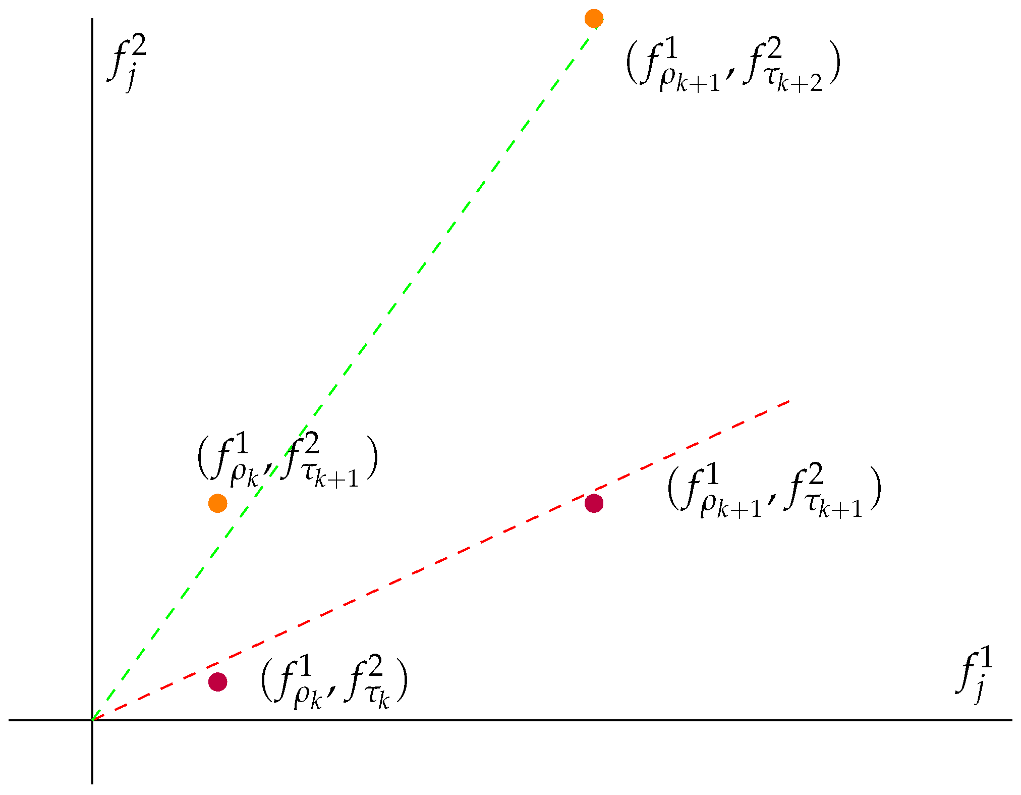
Theorem A2
(Dubins’ inequality for ratios, counting as per Definition A12). Let be a real-valued, non-negative trajectorial supermartingale (as per (A16)) and a positive sequence of non-anticipative functions. We require , for all and all j. For , consider the definitions of as given in Definition A12 and taking the value whenever the optimal conditioning sets are empty. Furthermore, assume that is such that -a.e. holds as per Definition A4; then, for any and ,
Therefore,
Proof.
For the purpose of the proof, we set , . We will prove , which will establish the results. Note that .
We note that the following inequality holds on :
where we used whenever (as well as ) and whenever . For later use, we rewrite (A21) as follows:
From Theorem 6.1 in [17], we obtain the following equality, being valid in the complement of a null set :
We refer to [17] for a description of the quantities appearing in the display above and note that is positive and arbitrary. Therefore, given that , the following inequality holds on :
where when and otherwise. Combining (A22) with (A23), we obtain
where whenever and otherwise. Applying to (A24) and using the facts that this functional preserves order, it is homogeneous, it is subadditive and , it follows that
which concludes the proof as is arbitrary. □
Theorem A2 relates to the previous discussion on small arbitrage by indicating that , where for a fixed but arbitrary parameter . By increasing k, we can achieve , where . As we explain below, trajectories belonging to represent pairs of price sequences that upcross a given cone in 2 dimensions. Theorem A2 proving is a novel 2-dimensional analog of the classical upcrossing inequality of Dubins ([32]).
To connect Theorem A2 with our 2-dimensional trajectory construction, we let and for the case where we only trade with in order to superhedge . This will guarantee that is a trajectorial martingale and hence a trajectorial supermartingale (as required in Theorem A2). That is, we formally rely on Theorem A2 in a 1-dimensional setting by considering the trajectory space consisting of trajectories ; this choice allows us to have access to [17] for sufficient conditions ensuring the validity of -a.e. (which is required in Theorem A2). Interestingly, the theorem does not require a supermartingale property for , and this allows one to apply the result within the 2-dimensional construction. One could formulate an alternative counting setting where both and are required to be supermartingales; such a formulation would place us in a genuinely 2-dimensional setting and would require dealing with -a.e. in 2 dimensions as well.
It then follows that Theorem A2 can be used to prune the two-dimensional trajectories by stopping their recursive construction whenever is considered to be sufficiently small. This can be done for each cone with . As explained above, this type of pruning is suggested a priori by the theoretical framework, which yields the novel cone crossing version of Dubins’ inequality stated in Theorem A2.
Appendix E. Use of AI Tools Declaration
The authors declare they have not used Artificial Intelligence (AI) tools in the creation of this article.
References
- Pfleiderer, P. Chameleons: The misuse of theoretical models in finance and economics. Rev. De Econ. Inst. 2014, 16, 23–60. [Google Scholar] [CrossRef] [Scilit]
- Feng, L.; Li, B.; Podobnik, B.; Preis, T.; Stanley, H.E. Linking agent-based models and stochastic models of financial markets. Proc. Natl. Acad. Sci. USA 2012, 109, 347–363. [Google Scholar] [CrossRef] [Scilit]
- Gajewski, K. Non-Probabilisitic Supermartingales. Trajectorial Models for Two Stocks. Ph.D. Thesis, Department of Mathematics, Toronto Metropolitan University, Toronto, ON, Canada, 2022. [Google Scholar] [CrossRef] [Scilit]
- Acciaio, B.; Beiglböck, M.; Penkner, F.; Schachermayer, W. A Model-Free Version of the Fundamental Theorem of Asset Pricing and the Super-Replication Theorem. Math. Financ. 2016, 26, 233–251. [Google Scholar] [CrossRef] [Scilit]
- Blanchard, R.; Carassus, L. No-arbitrage with multiple-priors in discrete time. Stoch. Process. Appl. 2020, 130, 6657–6688. [Google Scholar] [CrossRef] [Scilit]
- Bouchard, B.; Nutz, M. Arbitrage and duality in nondominated discrete-time models. Ann. Appl. Probab. 2015, 25, 823–859. [Google Scholar] [CrossRef] [Scilit]
- Burzoni, M.; Frittelli, M.; Hou, Z.; Maggis, M.; Oblooj, J. Pointwise arbitrage pricing theory in discrete time. Math. Oper. Res. 2019, 44, 1034–1057. [Google Scholar] [CrossRef] [Scilit]
- Burzoni, M.; Frittelli, M.; Maggis, M. Universal arbitrage aggregator in discrete-time markets under uncertainty. Financ. Stoch. 2016, 20, 1–50. [Google Scholar] [CrossRef] [Scilit]
- Burzoni, M.; Frittelli, M.; Maggis, M. Model-free superhedging duality. Ann. Appl. Probab. 2017, 27, 1452–1477. [Google Scholar] [CrossRef] [Scilit]
- Vovk, V. Continuous-time trading and the emergence of probability. Financ. Stoch. 2012, 16, 561–609. [Google Scholar] [CrossRef] [Scilit]
- Bartl, D.; Kupper, M.; Neufeld, A. Pathwise superhedging on prediction sets. Financ. Stoch. 2020, 24, 215–248. [Google Scholar] [CrossRef] [Scilit]
- Bartl, D.; Kupper, M.; Prömel, D.J.; Tangpi, L. Duality for pathwise superhedging in continuous time. Financ. Stoch. 2019, 23, 697–728. [Google Scholar] [CrossRef] [Scilit]
- Beiglböck, M.; Cox, A.M.G.; Huesmann, M.; Perkowski, N.; Promel, D.J. Pathwise superreplication via Vovk’s outer measure. Financ. Stoch. 2017, 21, 1141–1166. [Google Scholar] [CrossRef] [Scilit]
- Perkowski, N.; Prömel, D.J. Pathwise stochastic integrals for model free finance. Bernoulli 2016, 22, 2486–2520. [Google Scholar] [CrossRef] [Scilit]
- Vovk, V. Ito calculus without probability in idealized financial markets. Lith. Math. J. 2015, 55, 270–290. [Google Scholar] [CrossRef] [Scilit]
- Shafer, G.; Vovk, V. Game-Theoretic Foundations for Probability and Finance; Wiley: Hoboken, NJ, USA, 2019. [Google Scholar]
- Bender, C.; Ferrando, S.E.; Gajewski, K.; Gonzalez, A.L. Superhedging Supermartingales. Int. J. Approx. Reason. 2025, 187, 109567. [Google Scholar] [CrossRef] [Scilit]
- Liebrich, F.-B.; Maggis, M.; Svindl, G. Model Uncertainty: A Reverse Approach. SIAM J. Financ. Math. 2022, 13, 1230–1269. [Google Scholar] [CrossRef] [Scilit]
- Nutz, M. Robust superhedging with jumps and diffusion. Stoch. Process. Appl. 2015, 125, 4543–4555. [Google Scholar] [CrossRef] [Scilit]
- Carassus, L.; Gobet, E.; Teman, E. A class of financial products and models where super-replication prices are explicit. In Proceedings of the Ritsumeikan International Symposium on Stochastic Processes and Applications to Mathematical Finance; World Scientific: Singapore, 2006; pp. 67–84. [Google Scholar]
- Carassus, L.; Vargiolu, T. Super-replication price: It can be ok. Esaim Proc. Surv. 2018, 64, 54–64. [Google Scholar] [CrossRef] [Scilit]
- Kahale, N. Super-replication of financial derivatives via convex programming. Manag. Sci. 2017, 63, 2323–2339. [Google Scholar] [CrossRef] [Scilit]
- Britten-Jones, M.; Neuberger, A. Arbitrage pricing with incomplete markets. Appl. Math. Financ. 1996, 3, 347–363. [Google Scholar] [CrossRef] [Scilit]
- Ferro, S.E.; Fleck, A.; González, A.L.; Rubtsov, A. Trajectorial asset models with operational assumptions. Quant. Financ. Econ. 2019, 3, 661–708. [Google Scholar]
- Leinert, M. Daniell-Stone integration without the lattice condition. Arch. Math. 1982, 38, 258–265. [Google Scholar] [CrossRef] [Scilit]
- König, H. Integraltheorie ohne Verbandspostulat. Math. Ann. 1982, 258, 447–458. [Google Scholar] [CrossRef] [Scilit]
- Degano, I.L.; Ferrando, S.E.; González, A.L. Trajectory Based Market Models. Evaluation of Minmax Price Bounds. Dyn. Contin. Discret. Impuls. Syst. Ser. B Appl. Algorithms 2018, 25, 97–128. [Google Scholar]
- Degano, I.L.; Ferrando, S.E.; González, A.L. No-Arbitrage Symmetries. Acta Math. Sci. 2022, 42, 1373–1402. [Google Scholar] [CrossRef] [Scilit]
- van der Vaart, A.W.; Wellner, J.A. Weak Convergence and Empirical Processes; Springer: Berlin/Heidelberg, Germany, 1996. [Google Scholar]
- Vecer, J. Stochastic Finance. A Numeraire Approach; CRC Press: Boca Raton, FL, USA, 2011. [Google Scholar]
- Föllmer, H.; Schied, A. Stochastic Finance: An Introduction in Discrete Time, 3rd ed.; De Gruyter: Berlin, Germany, 2011. [Google Scholar]
- Neveu, J. Discrete-Parameter Martingales; North-Holland Mathematical Library; Elsevier: Amsterdam, The Netherlands, 1975. [Google Scholar]
- Dubins, L.E. A Note on Non-Negative Martingales. Ann. Appl. Probab. 1962, 33, 1365–1368. [Google Scholar]
- Burkholder, D.L. On the number of escapes of a martingale and its geometrical significance. In Almost Everywhere Convergence; Edgar, G.A., Sucheston, L., Eds.; Academic Press: New York, NY, USA, 1989; pp. 159–178. [Google Scholar]
- Schoutens, W.; Simons, E.; Tistaert, J. A Perfect Calibration! Now What? Best Wilmott 2005, 2, 281–304. [Google Scholar] [CrossRef] [Scilit]
- El Karoui, N.; Quenez, M. Dynamic programming and pricing of contingent claims in an incomplete market. SIAM J. Control Optim. 1995, 33, 29–66. [Google Scholar] [CrossRef] [Scilit]
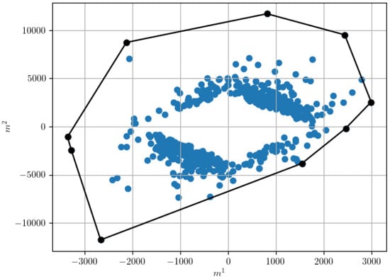
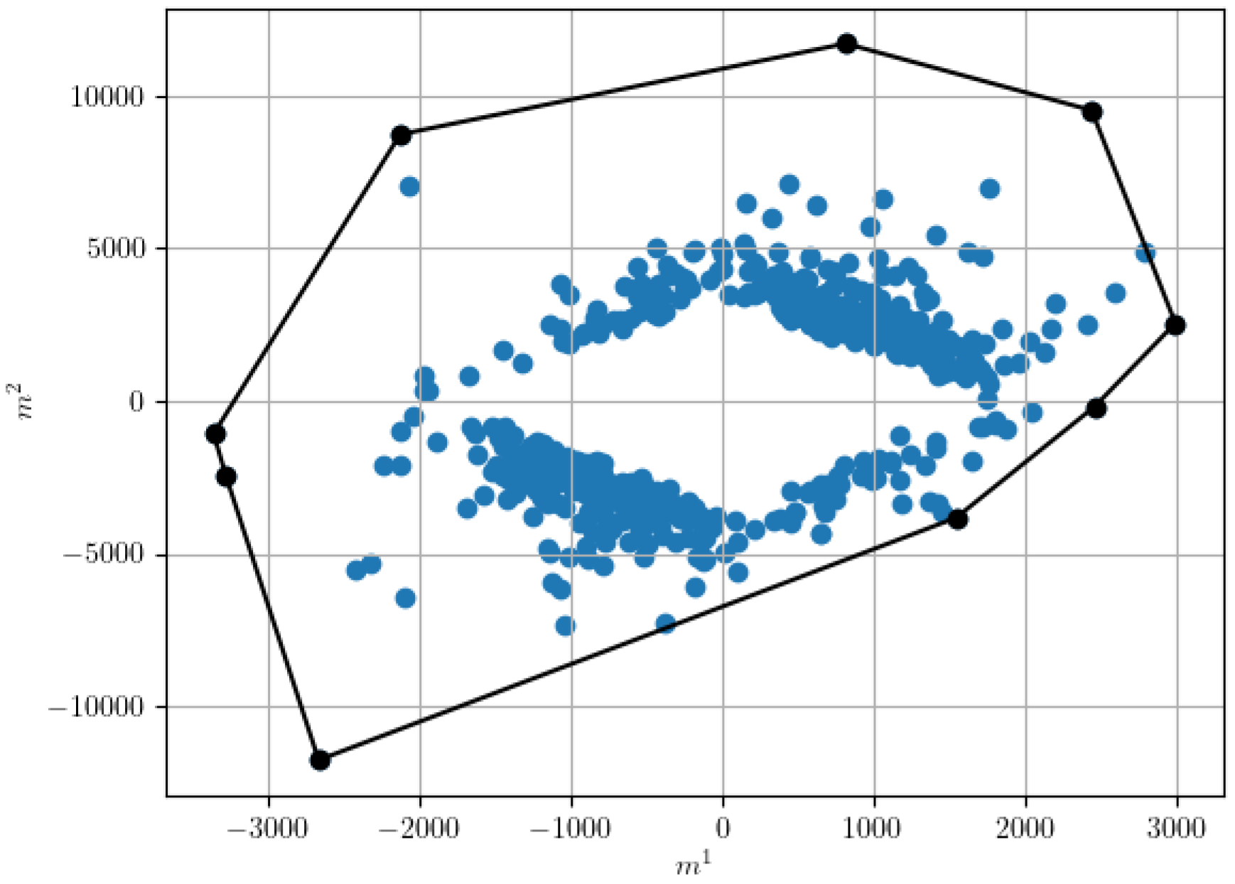
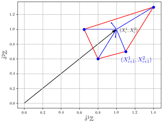
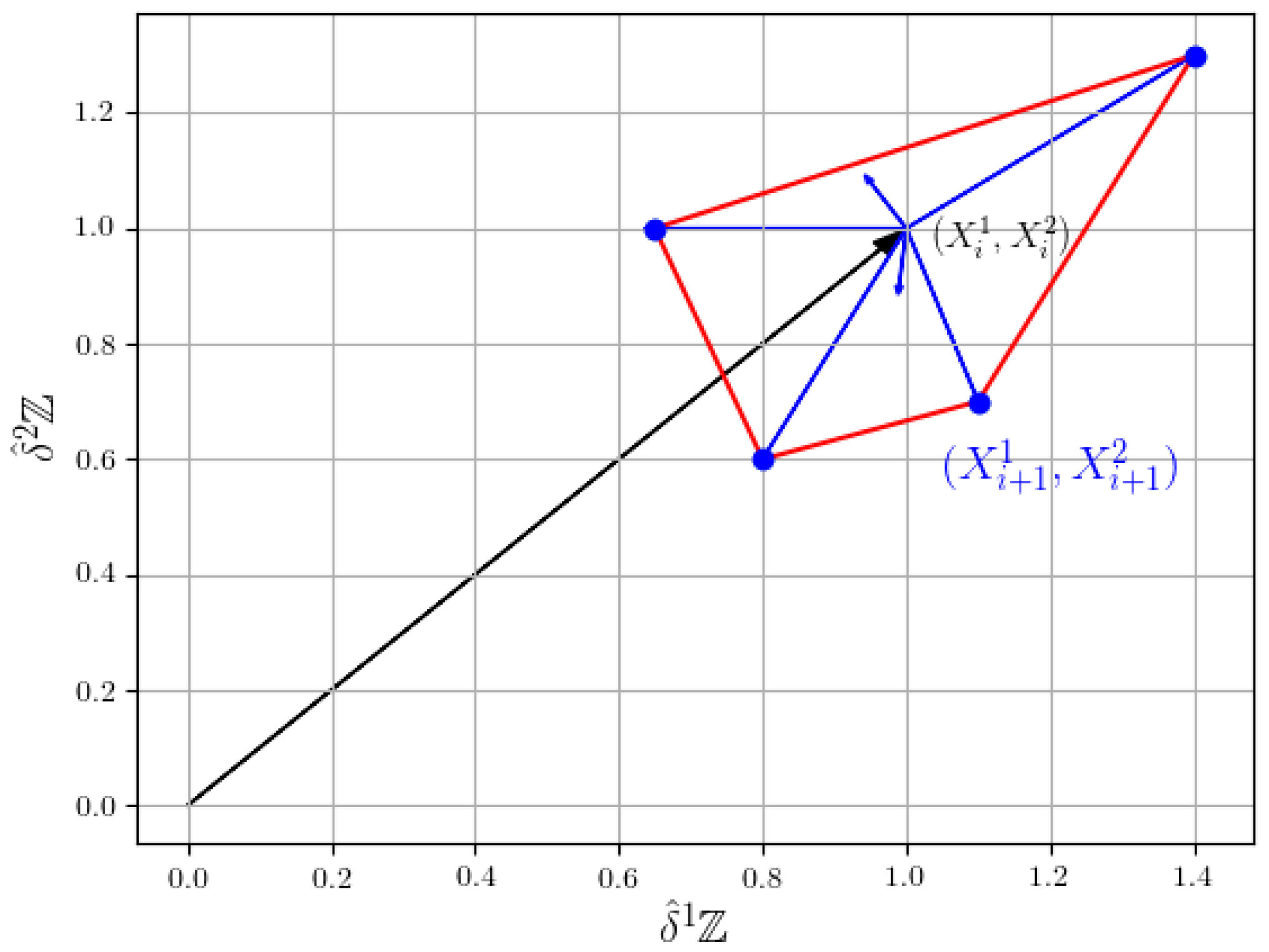
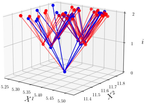
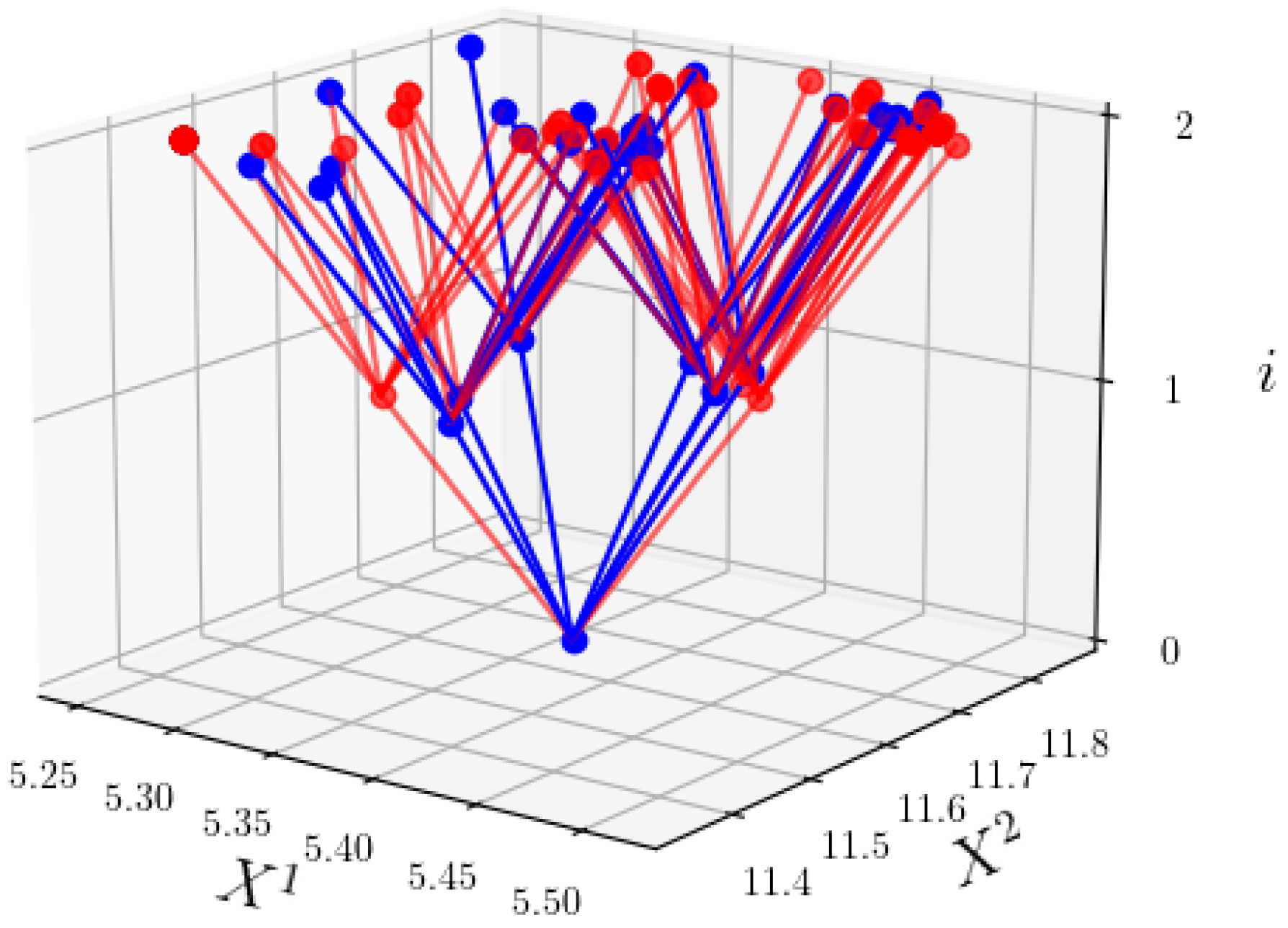
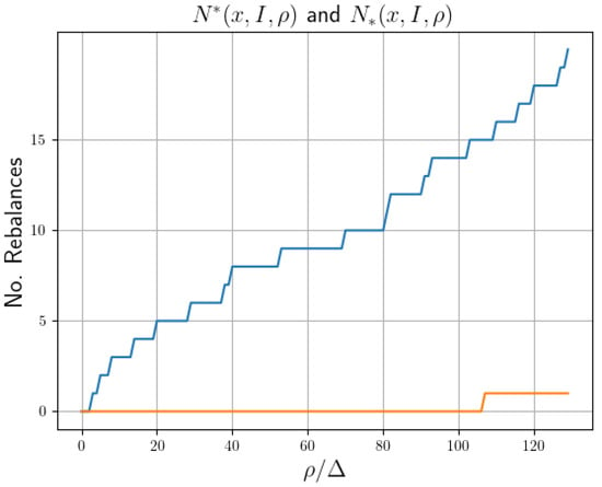
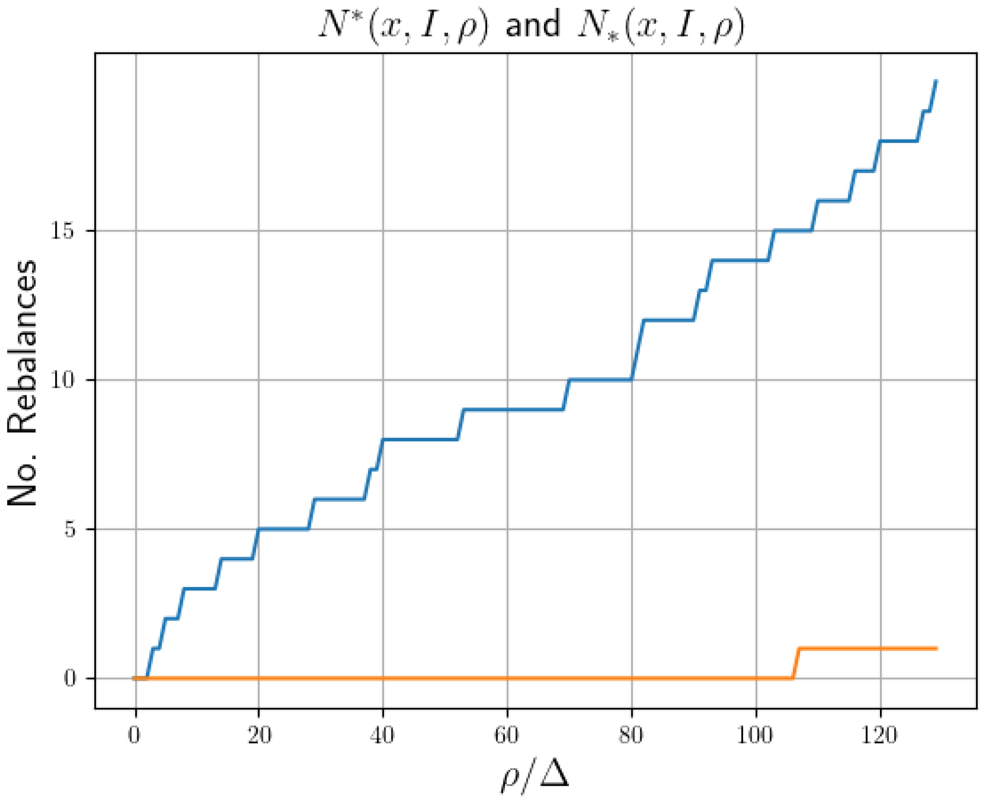
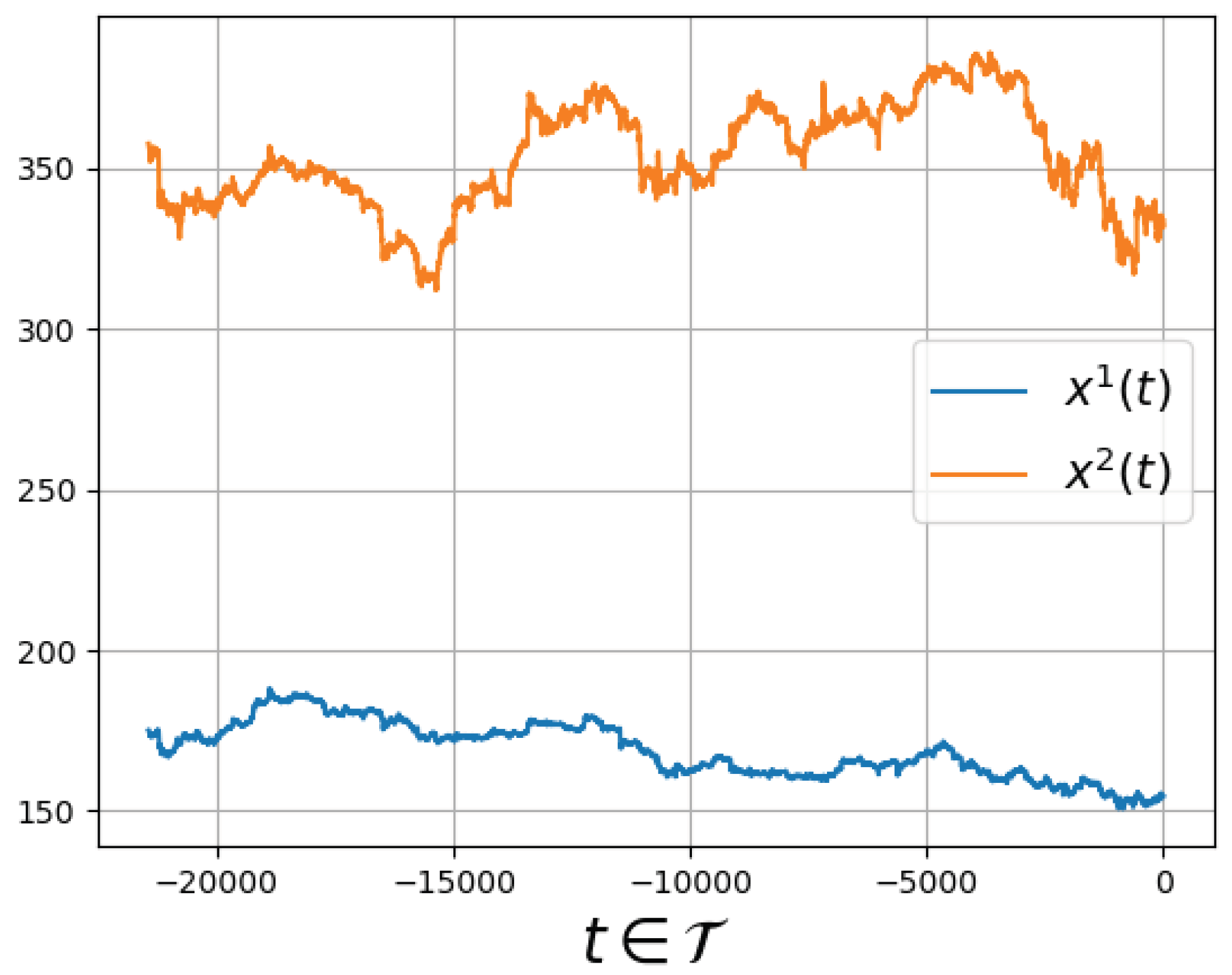
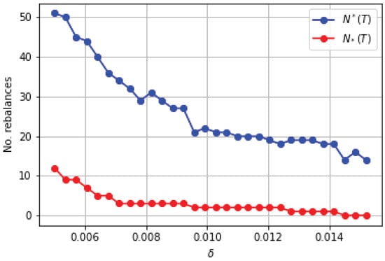
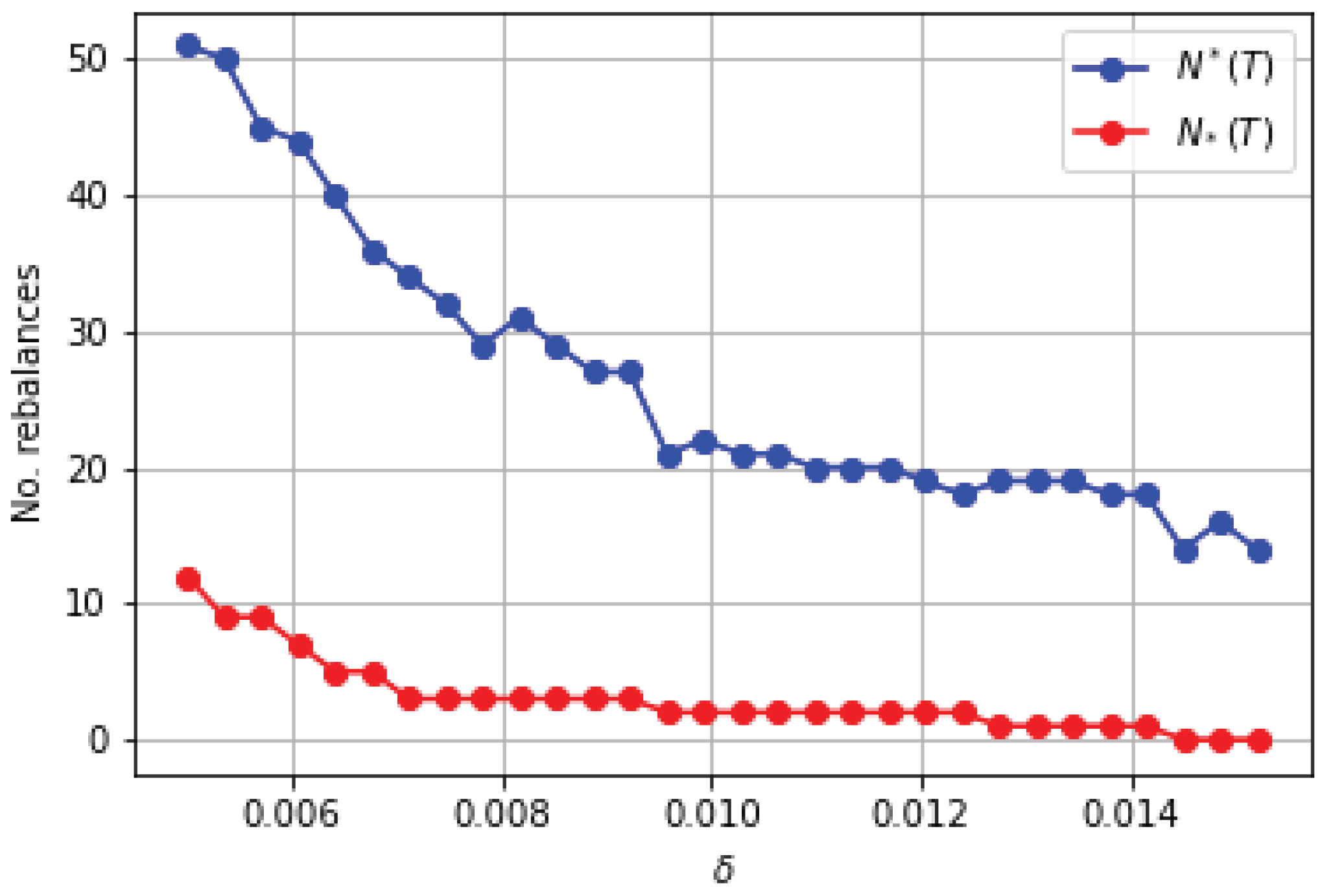
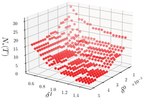
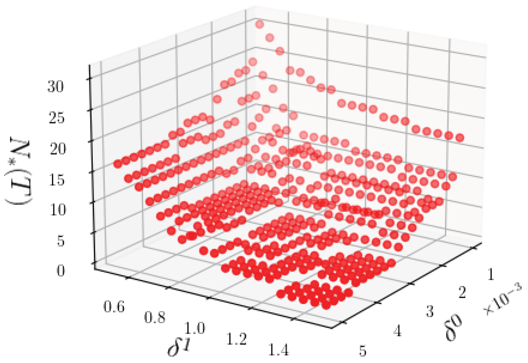
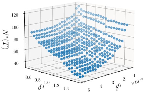
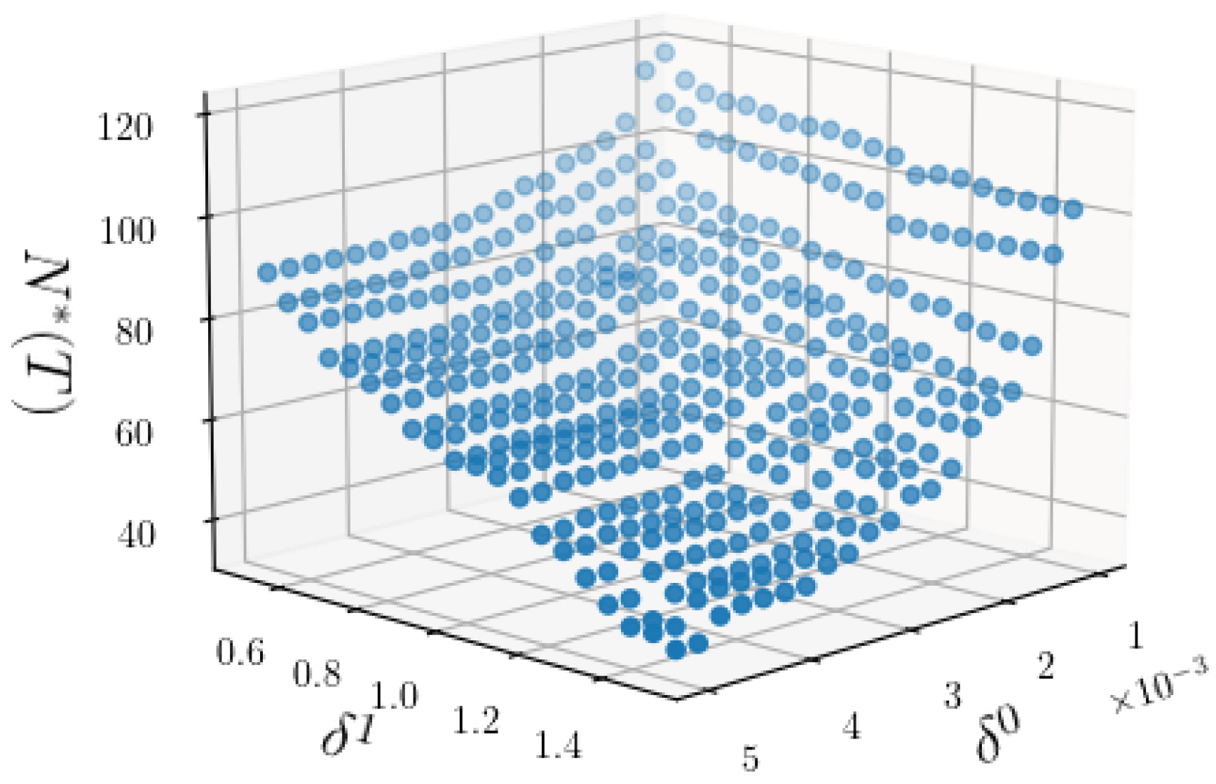
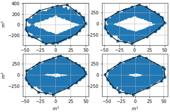
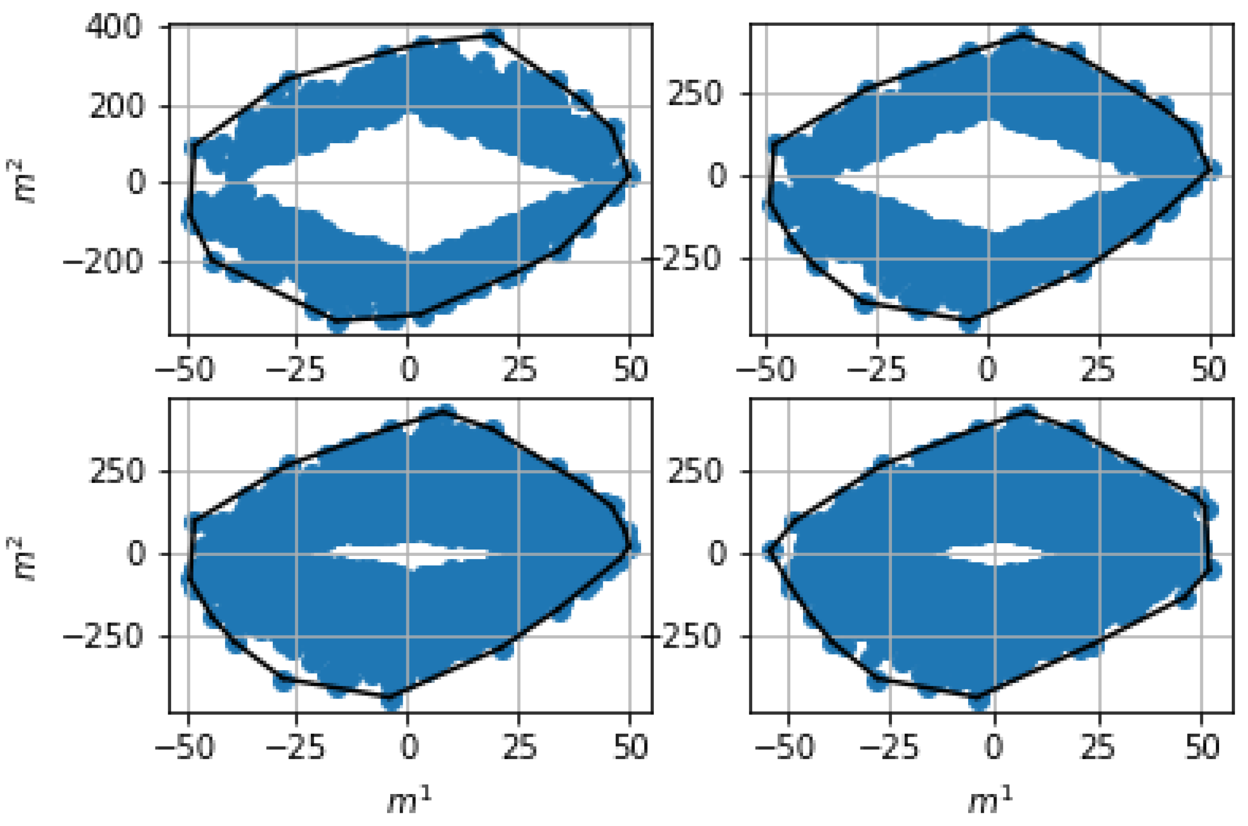
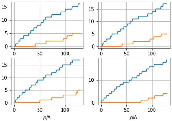
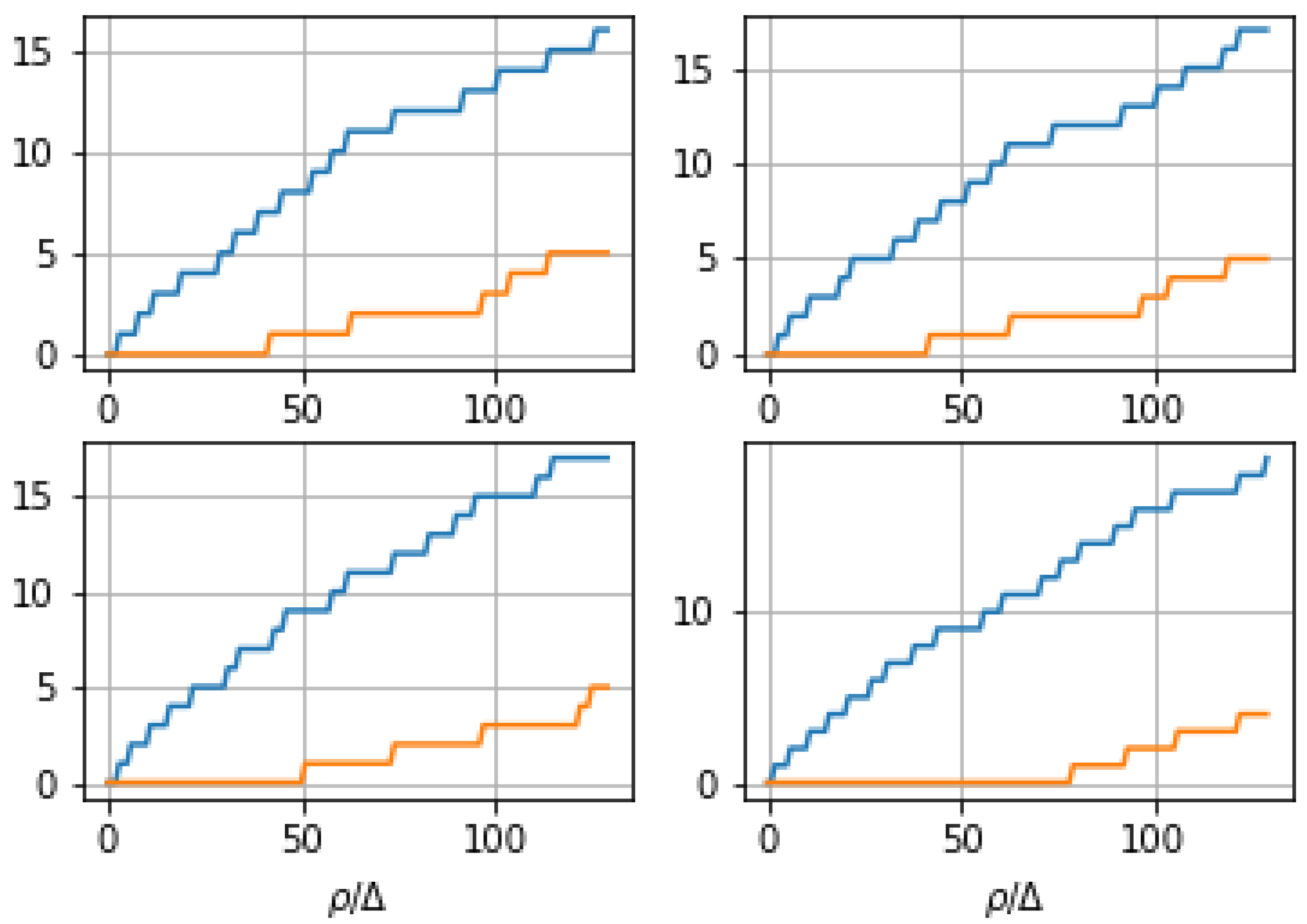
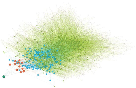
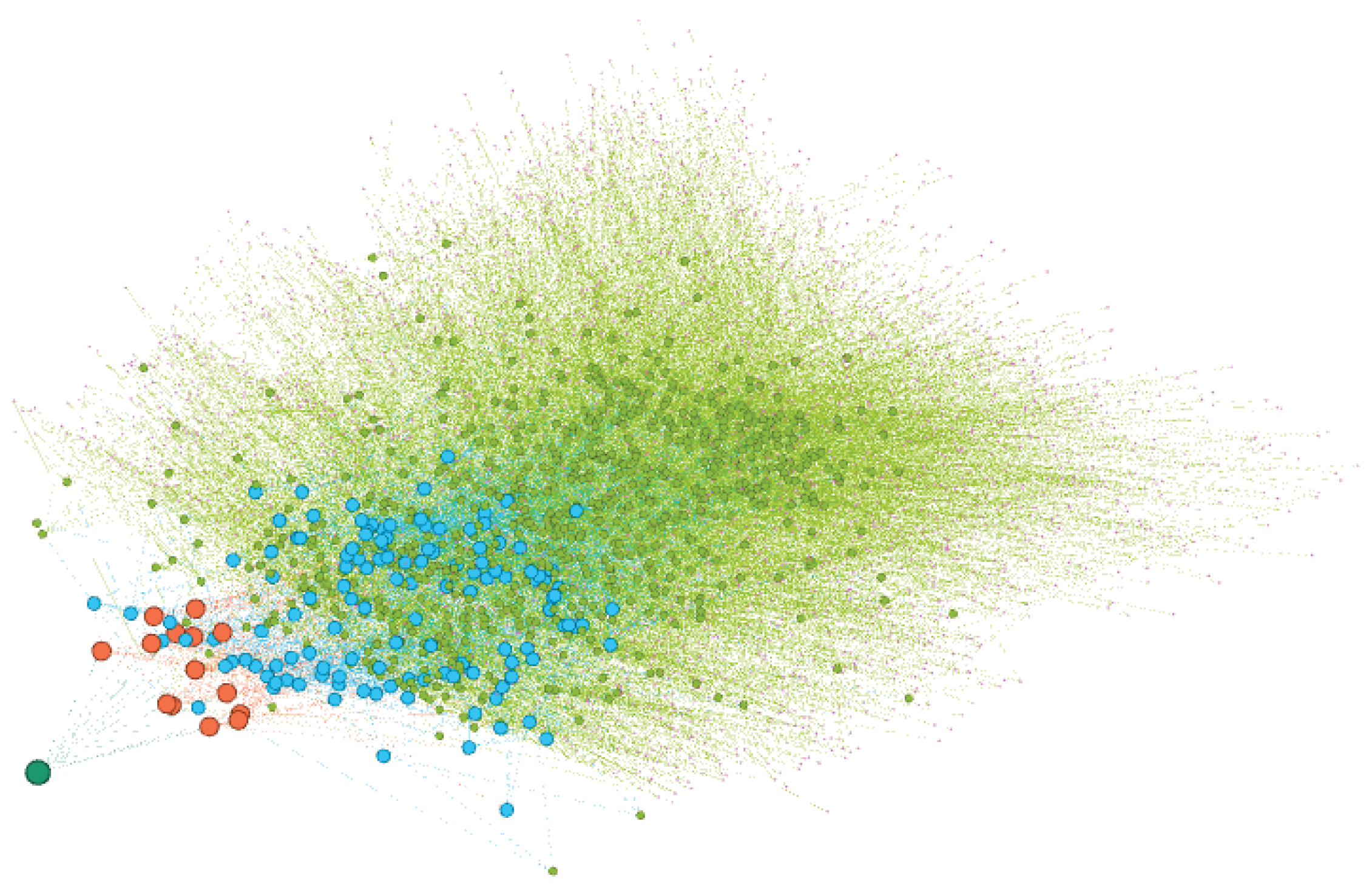
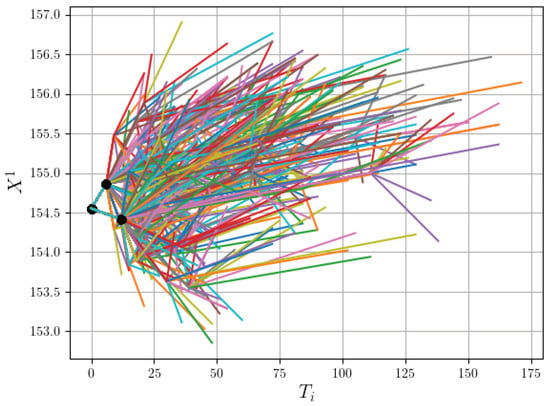
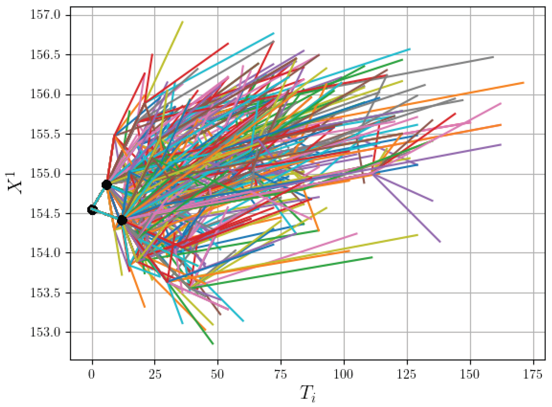
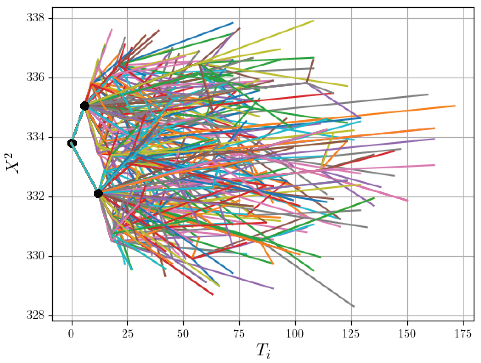
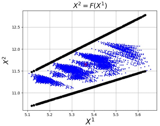
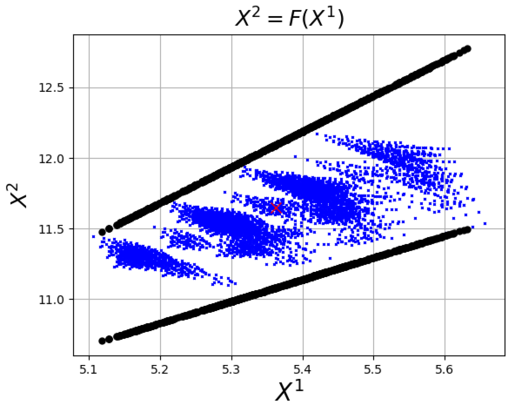
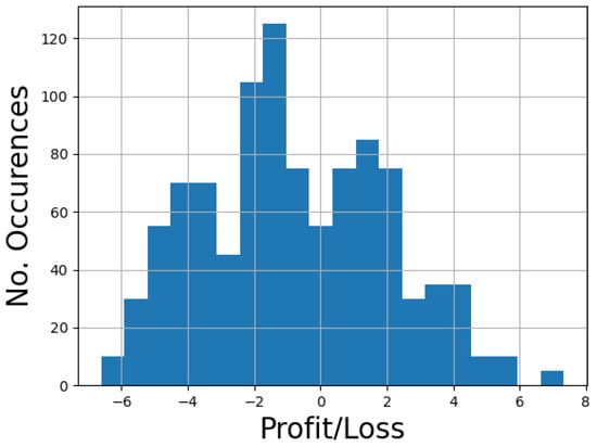
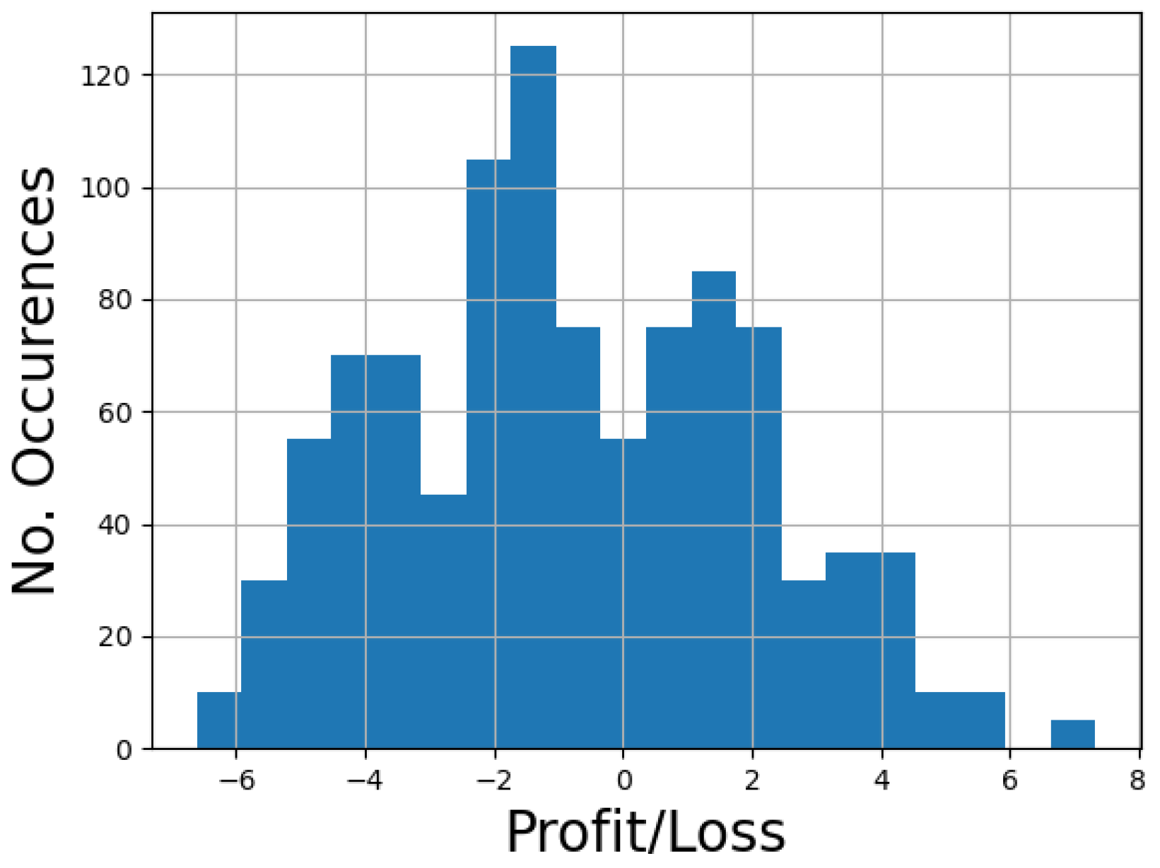
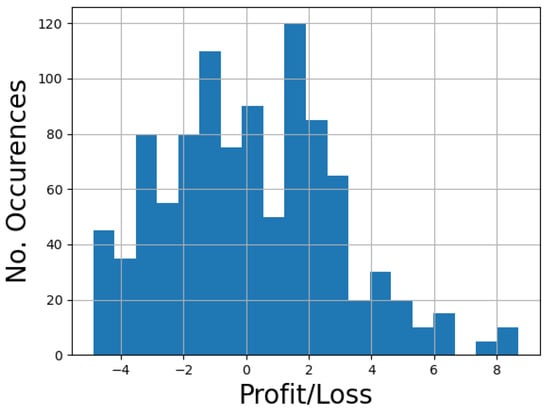
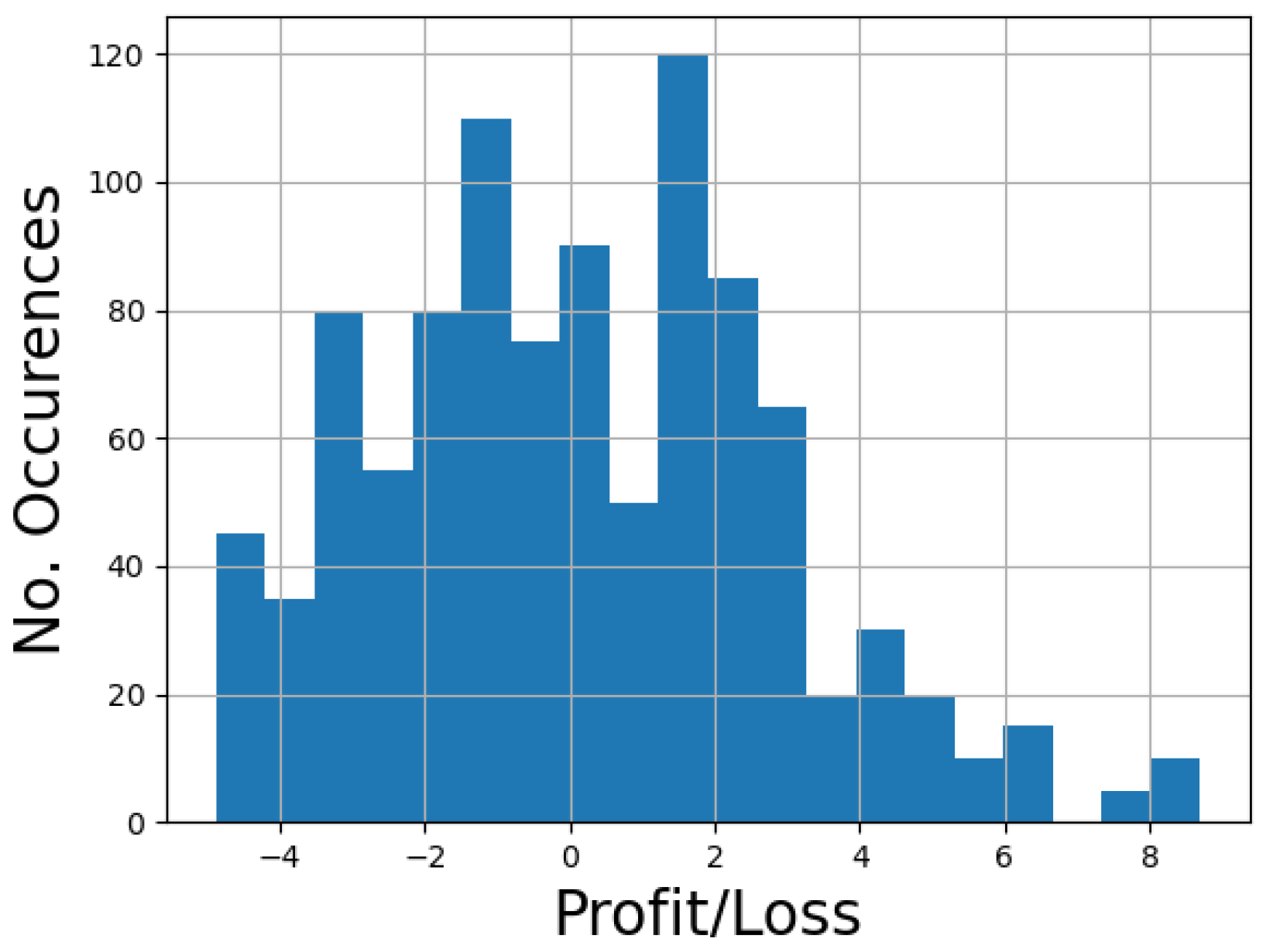
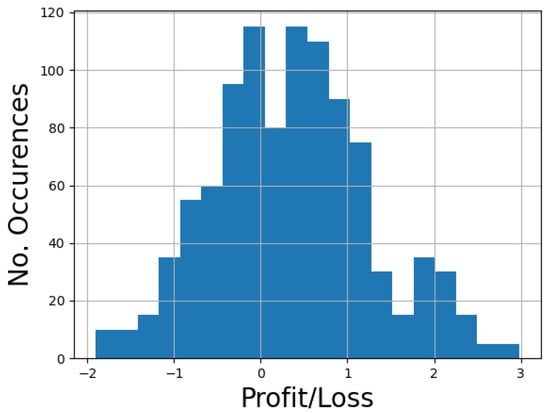
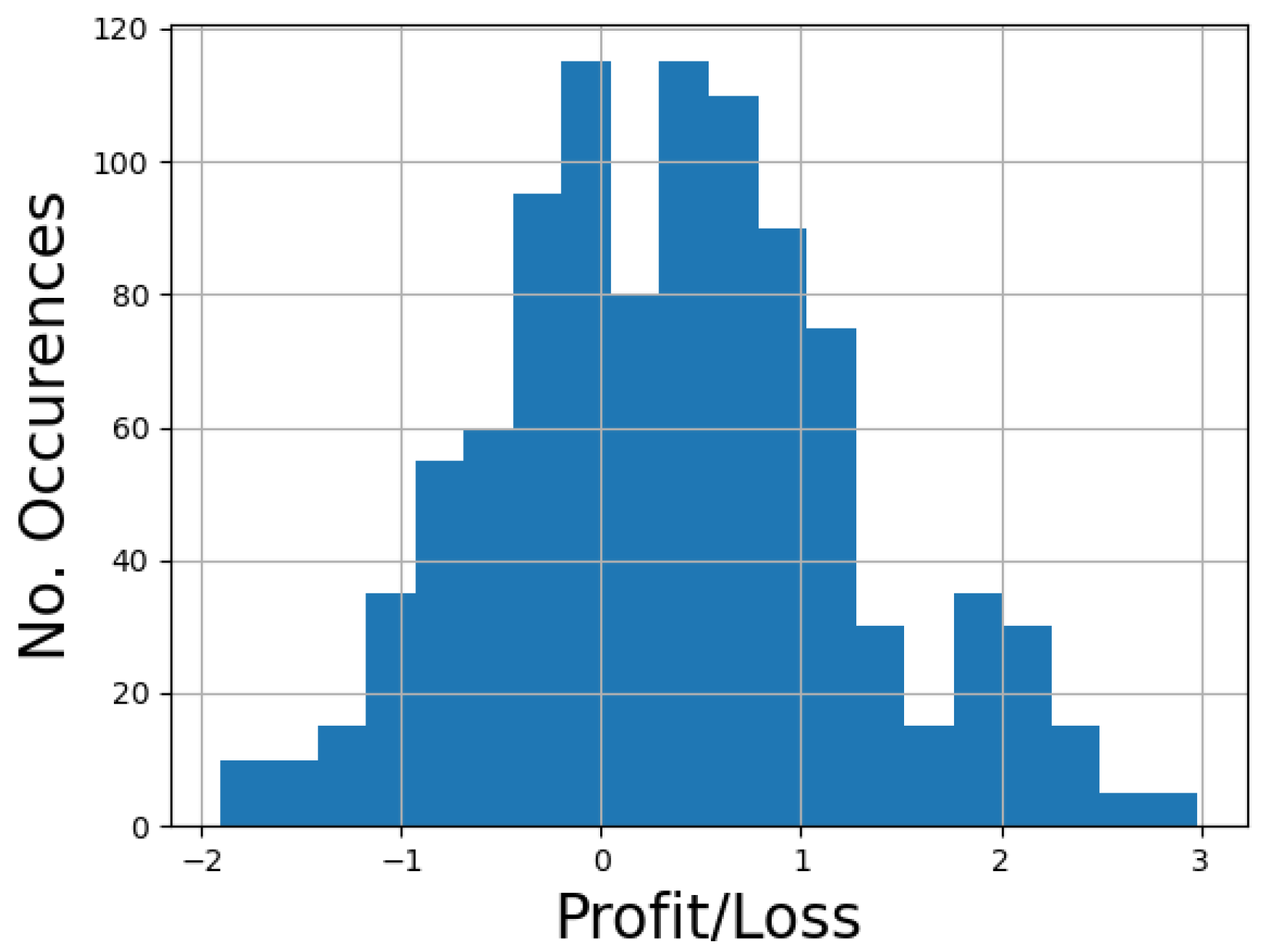
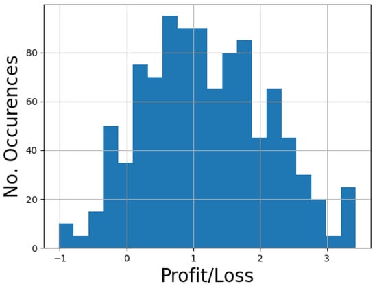
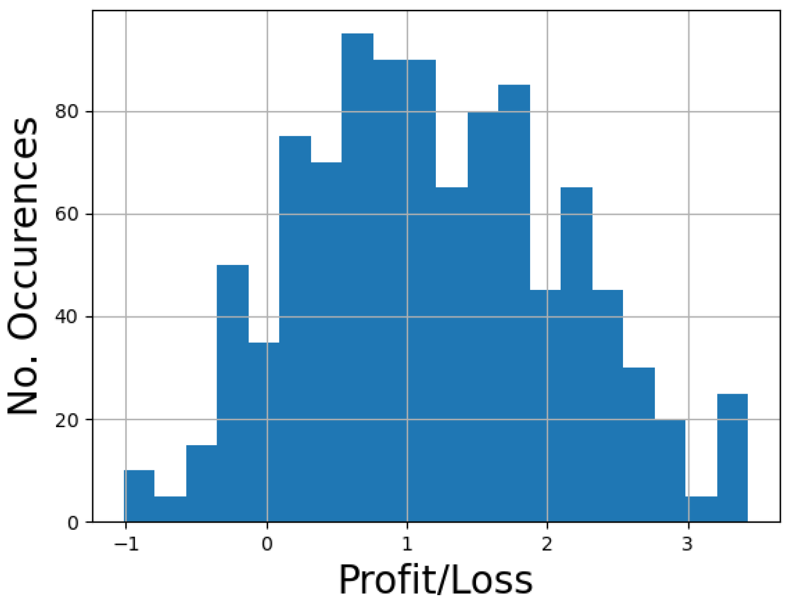
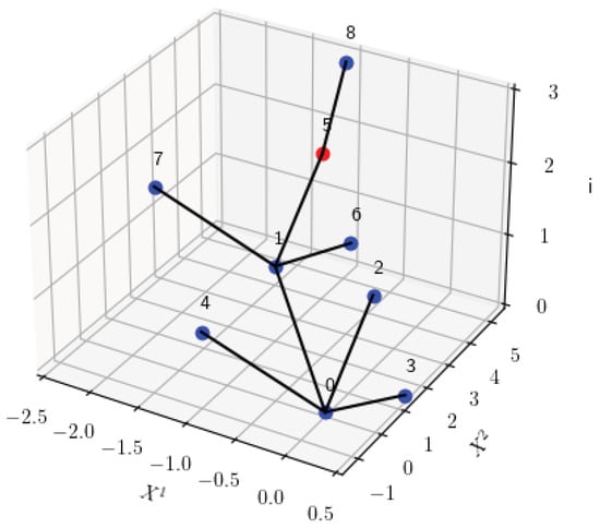
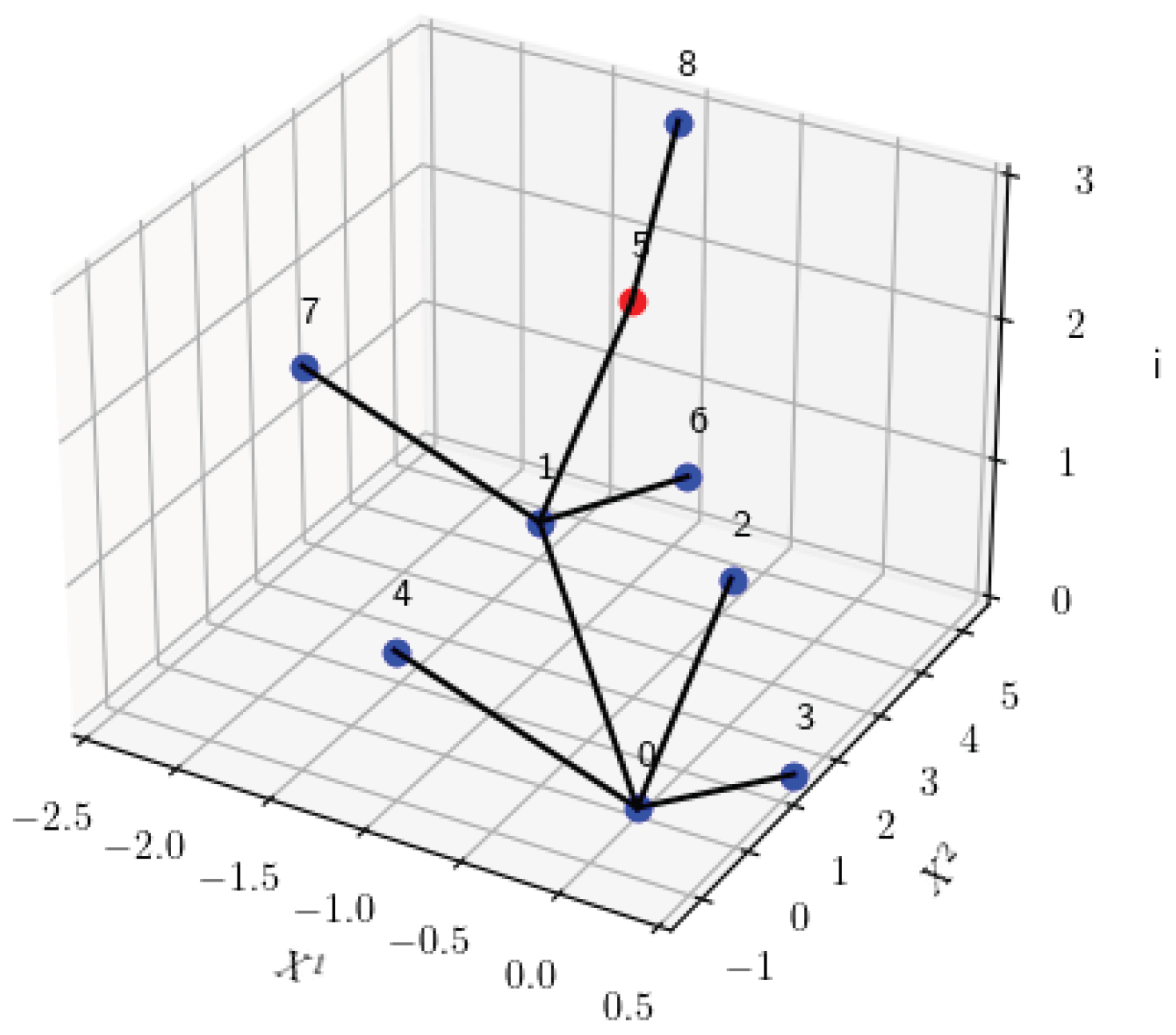
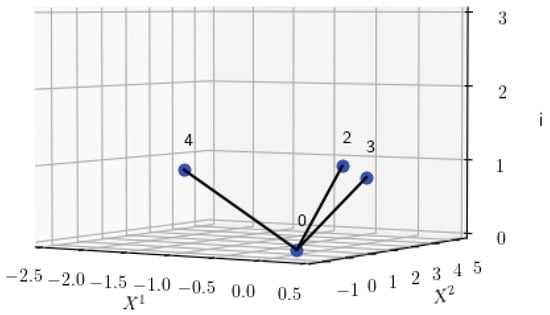
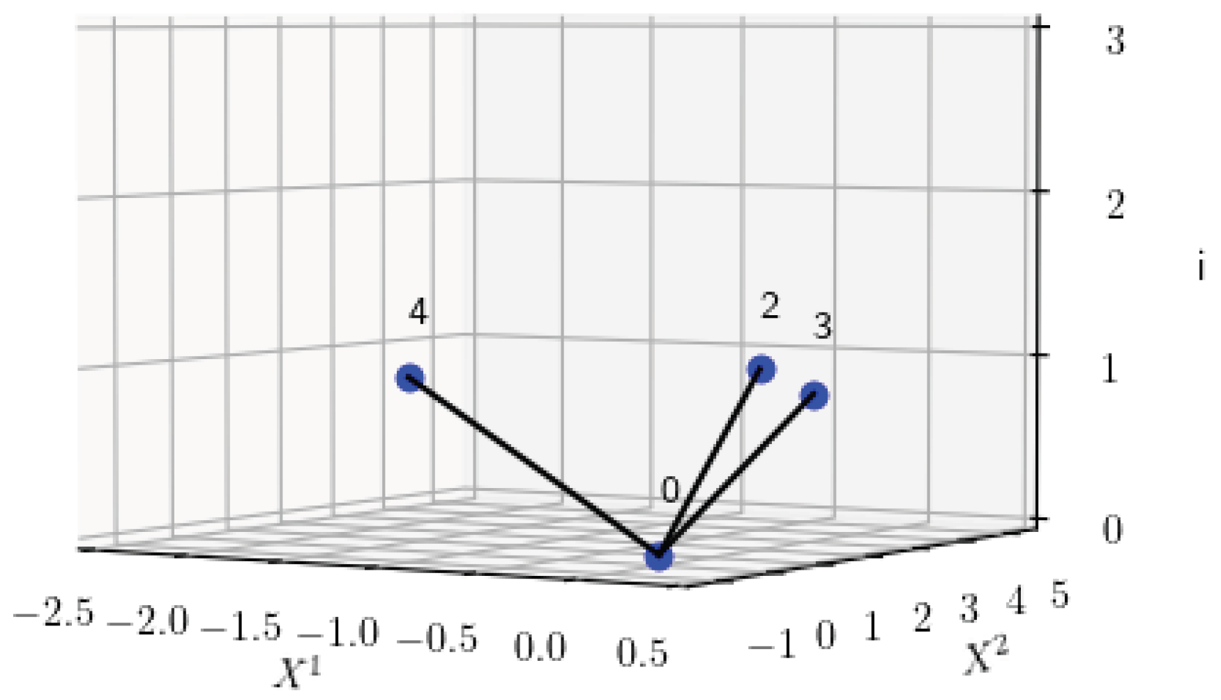
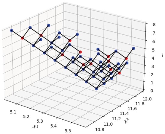
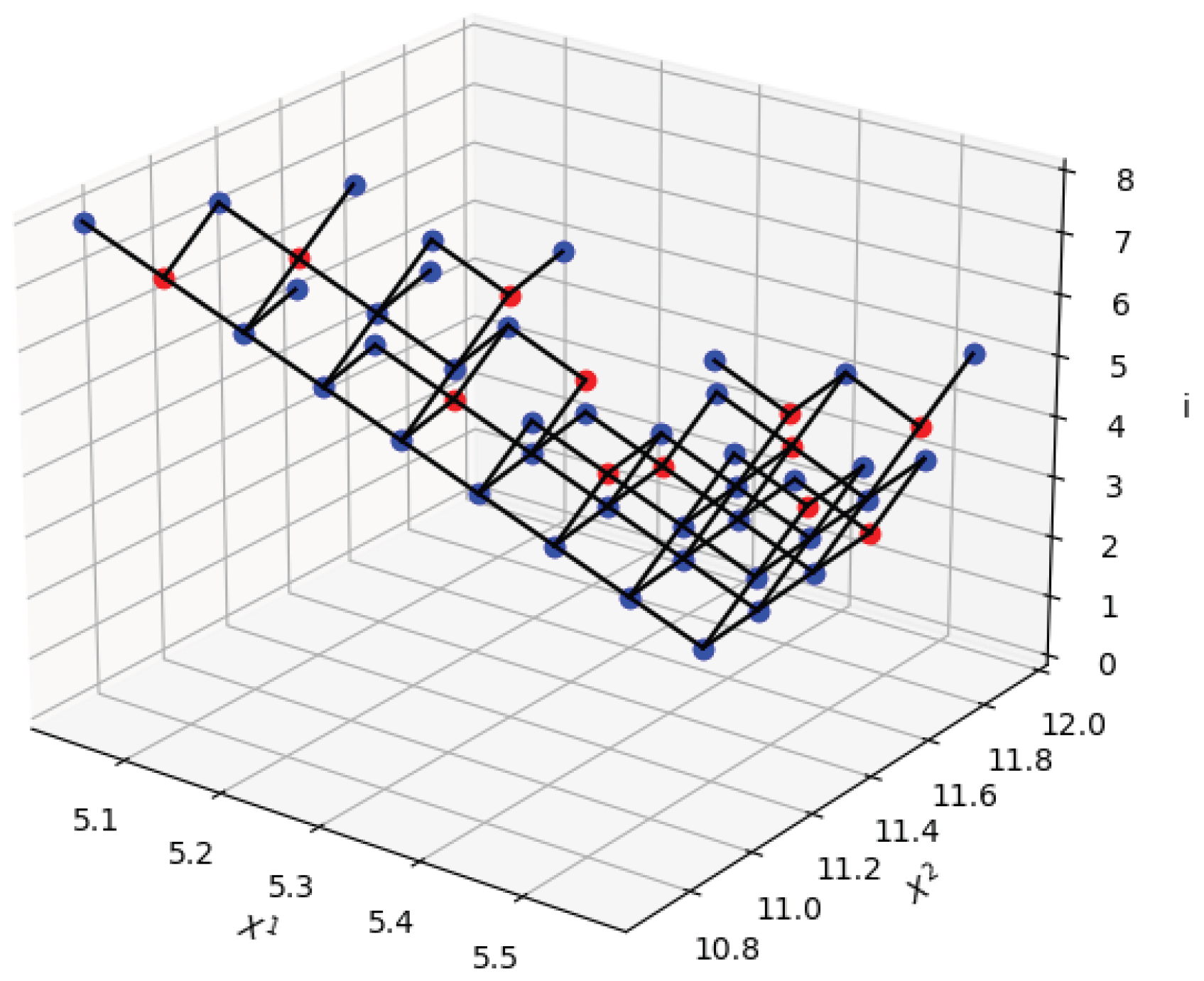

Disclaimer/Publisher’s Note: The statements, opinions and data contained in all publications are solely those of the individual author(s) and contributor(s) and not of MDPI and/or the editor(s). MDPI and/or the editor(s) disclaim responsibility for any injury to people or property resulting from any ideas, methods, instructions or products referred to in the content. |
© 2026 by the authors. Licensee MDPI, Basel, Switzerland. This article is an open access article distributed under the terms and conditions of the Creative Commons Attribution (CC BY) license.