Article

Stability and Direction of Hopf Bifurcation with Optimal Control Analysis of HIV Transmission Dynamics

by
Ibraheem M. Alsulami
1,* and
Fahad Al Basir
2,*
1
Mathematics Department, Faculty of Science, Umm Al-Qura University, Makkah 21955, Saudi Arabia
2
Department of Mathematics, Asansol Girls’ College, Dr. Anjali Roy Sarani, Asansol 713304, India
*
Authors to whom correspondence should be addressed.
Mathematics 2026, 14(6), 1079; https://doi.org/10.3390/math14061079
Submission received: 20 January 2026 / Revised: 18 March 2026 / Accepted: 20 March 2026 / Published: 23 March 2026

Abstract

In this study, we examine the effectiveness of combining interleukin-2 (IL-2) with highly active antiretroviral therapy (HAART) in controlling HIV replication. A mathematical model of the immune system is developed to analyze immune recovery when IL-2 is administered alongside HAART. We investigate the stability of the endemic equilibrium and Hopf bifurcation and determine the direction and stability of periodic solutions using center manifold theory. Numerical simulations are conducted to support the theoretical findings. The results show that the disease-free equilibrium is stable when the basic reproduction number  R 0 < 1 , while the endemic equilibrium exists when  R 0 > 1 . Our results also reveal the presence of a subcritical Hopf bifurcation in the system. An optimal control problem is also studied, showing that the combined therapy of IL-2 and HAART improves treatment outcomes, reduces side effects, and has a unique optimal control pair. Sensitivity analysis further highlights the importance of system parameters in influencing treatment effectiveness.

1. Introduction

AIDS (acquired immunodeficiency syndrome) can develop from HIV (human immunodeficiency virus), a chronic infection that targets the immune system, if treatment is not received [1]. Effective treatment enables people with HIV to live long, healthy lives even though there is no cure [2]. Significant advancements in long-acting treatments and cure-focused research are highlighted by recent HIV research. Clinical trials have shown promising results in both prevention and potential cures, and scientists are moving beyond daily pills to treatments that can be administered only twice a year [3]. Researchers have made great strides in 2025 with long-acting injectables and innovative PrEP options, which lessen the burden of daily medication and enhance adherence for HIV-positive individuals. Significant advancements in long-acting injectables and innovative PrEP options, which lessen the burden of daily medication and increase adherence for individuals living with HIV, have been reported by researchers in 2025. Data on a investigational twice-yearly regimen that combined lenacapavir with broadly neutralizing antibodies (bNAbs) was presented by Gilead Sciences. The regimen met its primary endpoint in Phase 2 trials and was designated as a breakthrough therapy [4]. The first HIV cure clinical trial, which was carried out in South Africa, also showed promising early results, highlighting the global movement toward functional cures [5]. These advancements are significant because they improve quality of life and advance the scientific community’s long-term objective of HIV eradication [6].
HIV transmission dynamics emphasize the critical role of highly active antiretroviral therapy (HAART) in reducing viral load and thereby lowering the probability of transmission. Mathematical models consistently show that HAART suppresses viral replication, driving the basic reproduction number ( R 0 ) below unity and stabilizing the system toward a disease-free equilibrium [7,8]. Interleukin-2 (IL-2), a cytokine that promotes CD4+ T-cell proliferation, has been investigated as an adjunct to HAART. Clinical trials have demonstrated that IL-2 administration increases CD4+ counts, enhancing immune reconstitution, though without significant improvement in long-term clinical outcomes compared to HAART alone [9,10]. Thus, while HAART directly reduces transmission risk by lowering viral load, IL-2 contributes indirectly by bolstering immune recovery, highlighting a complementary but limited role in transmission dynamics.
Mathematical modeling of viral dynamics provides a rigorous framework for designing therapeutic strategies and assessing the efficacy of antiviral interventions [11]. Extensive research has examined the global stability of models that capture the progression of viral infections, particularly in the context of HIV [12]. The host immune response is a critical determinant in limiting viral proliferation, and its modulation significantly influences disease outcomes. Modern antiretroviral agents are capable of suppressing viral replication and reducing immune activation, thereby mitigating apoptosis [13]. Nevertheless, while highly active antiretroviral therapy (HAART) has proven effective in controlling viral load, it only partially restores immune function. Complete eradication of HIV through HAART alone remains unattainable, as viral rebound typically occurs upon cessation of therapy. Consequently, there is growing interest in complementary therapeutic approaches, such as the administration of interleukin-2 (IL-2), which may enhance immune reconstitution and support long-term viral control [14,15,16].
Hopf bifurcation analysis is an important mathematical characteristic [17]. It is helpful in understanding the oscillatory behavior of human diseases, such as HIV infection dynamics [18]. Such oscillations, captured through Hopf bifurcation, provide insight into how treatment delays, cure rates, or immune saturation effects influence the persistence or suppression of HIV. Recent studies have rigorously examined these dynamics, showing that bifurcation thresholds mark transitions between stable infection states and oscillatory regimes, thereby offering valuable guidance for therapeutic strategies and long-term disease management [19].
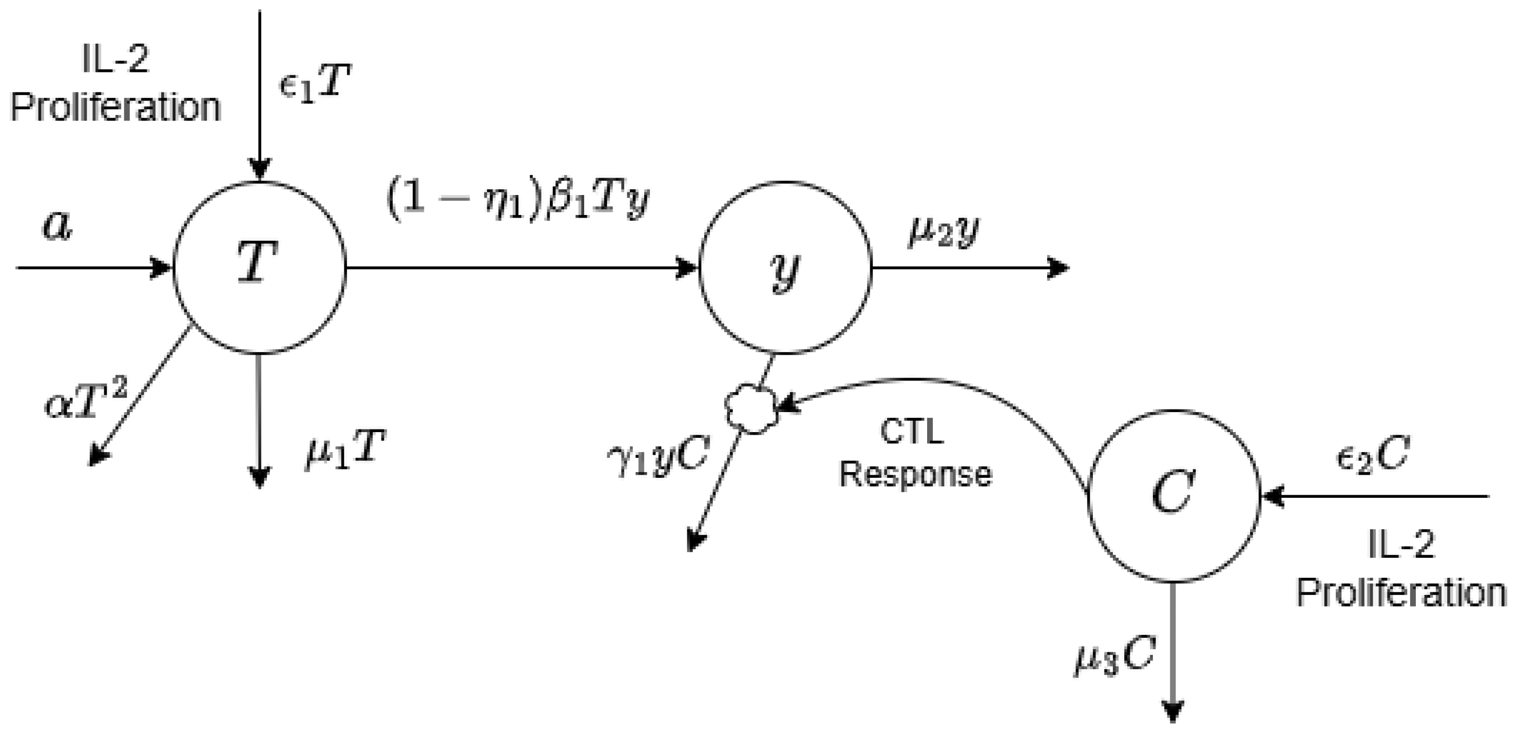
Interleukin-2 (IL-2) is a well-established cytokine that functions as a critical growth factor for T cells, regulating both their proliferation and differentiation across the entire T-cell compartment [20]. Following antigenic stimulation, IL-2 is secreted by CD4+ and CD8+ T-cell subsets within peripheral lymphoid organs, such as the spleen and lymph nodes. In the context of HIV infection, intermittent administration of highly active antiretroviral therapy (HAART), a therapeutic regimen primarily composed of reverse transcriptase inhibitors (RTIs) that block viral replication, has been proposed in combination with immune modulators like IL-2 [21,22]. Mechanistically, IL-2 enhances CD4+ T-cell activation, which can transiently reactivate latent HIV reservoirs. This reactivation allows cytotoxic T lymphocytes (CTLs) specific to HIV to recognize and eliminate infected cells, thereby contributing to viral clearance [17]. To provide a conceptual overview of this therapeutic interplay, we introduce Figure 1 to illustrate the relationship between HAART and IL-2-mediated immune modulation.
To better understand these complex interactions, mathematical models have been developed to simulate the effects of drug therapy in HIV patients. These models provide insights into viral dynamics, the emergence of drug resistance, and the decay kinetics of HIV-infected cellular compartments [23]. Furthermore, they have been applied to study thymic reconstitution in HIV-1 patients undergoing HAART, as well as to design optimal control strategies that integrate both HAART and IL-2 therapy [24]. Collectively, such modeling approaches highlight the potential of combining immunotherapy with antiretroviral treatment to improve long-term outcomes in HIV management.
Optimal control theory provides a rigorous mathematical framework for the design of drug administration strategies in HIV treatment, enabling researchers to balance therapeutic efficacy with the minimization of adverse side effects and economic costs [25]. By embedding drug scheduling protocols into dynamical models of HIV infection, one can formulate control functions that simultaneously suppress viral replication and preserve immune competence [26,27]. Within this context, the Pontryagin maximum principle (PMP) provides necessary conditions for optimality, allowing the derivation of adjoint equations and the construction of the Hamiltonian function that encapsulates system dynamics, control variables, and associated cost functionals [28]. The Hamiltonian formalism facilitates the identification of optimal trajectories for antiretroviral therapy (ART), guiding both dosage and timing decisions.
Recent studies have extended these models to incorporate compartments for remission, latent reservoirs, and patient adherence, thereby reflecting the complex biological and behavioral dimensions of HIV treatment [29,30]. Such analyses demonstrate that optimal control strategies, derived through PMP and Hamiltonian methods, can significantly improve long-term outcomes by reducing viral load while maintaining immune system integrity [26,27]. Boukary et al. [27] developed a mathematical model considering vertical transmission and applied optimal control to reduce the basic reproduction number and stabilize disease-free equilibria. Similarly, Rana et al. [31] introduced a deterministic SHATR model (susceptible–HIV infected–AIDS-infected–treatment–recovered) and used nonlinear stability analysis with control strategies to evaluate rehabilitation and treatment outcomes. More recently, Kumar et al. [32] emphasized stochastic elements in HIV spread, showing how optimal control can adapt drug interventions under uncertainty. Thus, mathematical modeling and optimal control are useful for disease management [33,34]. These approaches demonstrate that mathematical optimization not only refines drug application design but also enhances long-term treatment planning, offering insights into personalized therapy schedules and public health strategies.
Most past studies have mainly looked at stability and optimal control; they have not really explained things like repeating oscillations, limit cycles, or Hopf bifurcations. Some models that include time delays have studied these behaviors, but models without delays have not yet explored Hopf bifurcations, stability, or the direction of new periodic solutions. Also, when using optimal control methods, researchers have not checked whether the best control strategies are unique in the case of an HIV model for dynamics inside the body.
In this study, we undertake a comprehensive investigation of the reconstitution dynamics of CD4+ T cells and their regulatory influence on cytotoxic T lymphocytes (CTLs) in HIV-infected individuals undergoing highly active antiretroviral therapy (HAART) in conjunction with interleukin-2 (IL-2) administration. The proposed mathematical modeling framework is designed to elucidate the interactions among distinct T lymphocyte subsets during HIV progression and to determine optimal conditions for immune-based therapeutic strategies associated with HAART. Moreover, the framework integrates principles of optimal control theory to inform the rational scheduling of IL-2 as an adjuvant therapy alongside HAART, with the overarching objective of enhancing immune restoration, suppressing viral persistence, and ultimately advancing toward a functional cure.

2. Model Formulation with Drugs

We formulate the mathematical model for the dynamics of HIV infection within a human body with the following assumptions:
A1: 
We consider a dynamical system describing the interaction between uninfected CD4+ T cells, infected CD4+ T cells, and cytotoxic T lymphocytes (CTLs). Let us define the model populations:
(i)
The density of uninfected CD4+ T cells, T(t);
(ii)
The density of infected CD4+ T cells, y(t);
(iii)
The density of CTL cells, C(t), at any time t.
The interactions among the populations are discussed below. The model is built upon several biological and pharmacological assumptions that govern the dynamics of CD4+ T cells and cytotoxic T lymphocytes (CTLs) under HIV infection and drug treatment.
A2: 
We assumed that uninfected CD4+ T cells undergo natural apoptosis at a constant rate denoted by  μ 1 , while CTLs similarly die at a rate  μ 3  [35]. Due to spatial and resource limitations within the host environment, uninfected CD4+ T cells also experience intra-population competition, which is captured by a quadratic term  α T 2  [36,37].
A3: 
The infection process is modeled as being proportional to the frequency of encounters between uninfected and infected CD4+ T cells, with an infection rate  β 1 0  [8]. The presence of reverse transcriptase inhibitors (RTIs) reduces this infection rate by a factor of  ( 1 η 1 ) , where  η 1 [ 0 , 1 ]  represents the efficacy of RTI treatment [38]. However, as emphasized in the introduction, this formulation explicitly captures the RTI aspect of HAART. Interleukin-2 (IL-2) therapy is also incorporated into the model to account for its role in enhancing the proliferation of CD4+ T cells, represented by the term  ε 1 T  [9,39,40] (as indicated by Figure 1).
A4: 
On the immune response side, CTLs are responsible for eliminating infected CD4+ T cells, and this cytotoxic activity is modeled as being proportional to the contact rate between CTLs and infected cells, with a removal rate  γ 1  [15]. Furthermore, CTLs proliferate in response to the presence of infected cells at a rate  γ 2  [15], and this proliferation is further boosted by IL-2 treatment, captured by the term  ε 2 C  [41].
These assumptions collectively define the interactions and regulatory mechanisms within the immune system under therapeutic intervention, forming the basis for the system of differential equations that describe the model.
The resulting system of ordinary differential equations is given by
T ˙ ( t ) = a μ 1 T α T 2 ( 1 η 1 ) β 1 y T + ε 1 T , y ˙ ( t ) = ( 1 η 1 ) β 1 y T μ 2 y γ 1 y C , C ˙ ( t ) = γ 2 y C μ 3 C + ε 2 C ,
with initial conditions
T ( 0 ) = T 0 > 0 , y ( 0 ) = y 0 > 0 , C ( 0 ) = C 0 > 0 .
The parameters of the model (1) can assume the following values:  a > 0 μ 1 > 0 ,   β 1 0 ,   γ 2 0 ϵ 1 , ϵ 2 > 0 ,   μ 2 , μ 3 > 0 , and  η 1 [ 0 , 1 ] . Short descriptions and baseline values of the parameters are mentioned in Table 1.

3. Basic Properties

We now analyze the qualitative properties of the system (1) with respect to the existence, uniqueness, and positivity of solutions.

3.1. Existence and Uniqueness of Solutions

The right-hand side of the system (1) is a polynomial in  ( T , y , C )  and hence belongs to  C ( R 3 ) . Therefore, it is locally Lipschitz continuous on  R 3 . According to the Picard–Lindelöf Theorem [44,45], for any initial condition  ( T 0 , y 0 , C 0 ) R 3 , there exists a unique local solution.

3.2. Positive Invariance

From the second equation of (1),
y ˙ = ( 1 η 1 ) β 1 T μ 2 γ 1 C y ,
which is linear in y. Thus, we have
y ( t ) = y ( 0 ) exp 0 t ( 1 η 1 ) β 1 T ( s ) μ 2 γ 1 C ( s ) d s .
If  y ( 0 ) = 0 , then  y ( t ) 0 . If  y ( 0 ) > 0 , then  y ( t ) > 0  for all t in the interval of existence. Hence  y ( t ) 0  for all  t 0 . Similarly, the third equation of (1) is linear in C:
C ˙ = γ 2 y μ 3 + ε 2 C ,
yielding
C ( t ) = C ( 0 ) exp 0 t γ 2 y ( s ) μ 3 + ε 2 d s .
Thus  C ( t ) 0  for all  t 0  whenever  C ( 0 ) 0 .
We show the nonnegativity of  T ( t )  by contradiction. Consider the differential equation
T ˙ ( t ) = a + ( ε 1 μ 1 ) T ( t ) α T ( t ) 2 ( 1 η 1 ) β 1 y ( t ) T ( t ) ,
with initial condition  T ( 0 ) > 0  and parameter  a > 0 .
We assume, for the sake of contradiction, that there exists a time  t * > 0  such that
T ( t * ) < 0 .
Since  T ( 0 ) > 0  and  T ( t )  is continuous, there must exist a first time  τ > 0  such that
T ( τ ) = 0 , and T ( t ) > 0 for all 0 t < τ .
At  t = τ , substituting  T ( τ ) = 0  into the differential equation yields
T ˙ ( τ ) = a .
As  a > 0 , then  T ˙ ( τ ) > 0 , meaning that  T ( t )  is increasing from the boundary. Thus,  T ( t )  cannot cross into the negative region.
Therefore, the solution cannot cross below zero at  τ . This contradicts the assumption that  T ( t * ) < 0  for some  t * > 0 . Hence, the contradiction shows that
T ( t ) 0 for all t 0 ,
provided  T ( 0 ) > 0  and  a 0 .

3.3. Boundedness of the System

The right-hand side of the system (1) consists of smooth polynomial functions in the variables T, y, and C, together with the system parameters. Therefore, local existence, uniqueness, and continuity of solutions are guaranteed [44,45]. In this subsection, we establish that the solutions of the system are uniformly bounded under suitable parameter conditions.
Theorem 1.
Let  X ( t ) = ( T ( t ) , y ( t ) , C ( t ) )  be a solution of (1) with nonnegative initial data. If  μ 1 > ε 1  and  μ 3 > ε 2 + γ 2 y ( 0 ) μ 2 > ( 1 η 1 ) β 1 T m T m = max T ( 0 ) , a μ 1 ε 1 ,  then  X ( t )  is uniformly bounded for all  t 0 .
Proof. 
Firstly, we consider the first equation of (1) to obtain the inequality
d T d t a ( μ 1 ε 1 ) T .
This is a linear differential inequality. By the comparison theorem [46], we can write
T ( t ) max T ( 0 ) , a μ 1 ε 1 : = T m , t 0 .
Thus,  T ( t )  is bounded for all  t > 0 . For the boundedness of  y ( t ) , we recall
y ˙ = ( 1 η 1 ) β 1 T μ 2 γ 1 C y ,
which implies
d y d t ( 1 η 1 ) β 1 T m μ 2 y .
Thus,  y ( t )  is bounded by  y ( 0 )  provided that  ( 1 η 1 ) β 1 T m μ 2 < 0 .
For the boundedness of  C ( t ) , we consider the third equation of (1)
C ˙ = ( γ 2 y μ 3 + ε 2 ) C .
This gives
d C d t ( γ 2 y m μ 3 + ε 2 ) C
Since  μ 3 > ε 2 , the coefficient of C is bounded above by  C ( 0 )  provided that  γ 2 y m μ 3 + ε 2 < 0 .
Combining these results, we conclude that  X ( t ) = ( T ( t ) , y ( t ) , C ( t ) )  is uniformly bounded for all  t 0  if  μ 1 > ε 1  and  μ 3 > ε 2 + γ 2 y m . □

3.4. Equilibrium Analysis

We now determine the equilibrium points of system (1). The model (1) admits three equilibria, namely the following:
(i)
The disease-free equilibrium  E DF T DF , 0 , 0 ,  where
T DF = ( ε 1 μ 1 ) + ( ε 1 μ 1 ) 2 + 4 α a 2 α ,
(ii)
The CTL-free endemic equilibrium  E CF T C F , y C F , 0 , where
y C F = a + ( ε 1 μ 1 ) T C F α ( T C F ) 2 ( 1 η 1 ) β 1 T C F , T C F = μ 2 ( 1 η 1 ) β 1 .
E CF  is feasible if  y C F > 0 .
(iii)
The endemic equilibrium  E EE T E E , y E E , C E E ,  where
T E E = Δ + Δ 2 + 4 α a 2 α ,
y E E = μ 3 ε 2 γ 2 ,
C E E = ( 1 η 1 ) β 1 T E E μ 2 γ 1 ,
with  Δ = ε 1 μ 1 ( 1 η 1 ) β 1 μ 3 ε 2 γ 2 E EE  is biologically feasible if
T E E > μ 2 / ( ( 1 η 1 ) β 1 ) , and μ 3 > ε 2 .

3.5. The Basic Reproduction Number,  R 0

In this section, we derive the basic reproduction number  R 0  using the next-generation matrix (NGM) method [47,48]. We follow the standard framework in which  R 0  is defined as the spectral radius of  F V 1 , where F collects the rate of appearance of new infections and V collects the transition terms out of infected compartments.
Here, we note that the DFE is  ( T DF , 0 , 0 ) , where
T DF = ( ε 1 μ 1 ) + ( ε 1 μ 1 ) 2 + 4 α a 2 α .
Now, we choose the infected compartments. The only epidemiologically infected compartment is the population of infected CD4+ T cells, y. CTLs (C) mediate immune response but are not infected states; T represents susceptible/uninfected CD4+ T cells. Therefore, the infected subsystem is one-dimensional with state y.
We write the differential equation for y as follows:
y ˙ = ( 1 η 1 ) β 1 T y F ( y ) μ 2 + γ 1 C y V ( y ) .
At the DFE  E 0 ( T DF , 0 , 0 ) , the linearization of F and V with respect to y is the as follows:
F = y ( 1 η 1 ) β 1 T y DFE = ( 1 η 1 ) β 1 T DF , V = y ( μ 2 + γ 1 C ) y DFE = μ 2 .
Since the infected subsystem is one-dimensional, the next-generation matrix  F V 1  reduces to the scalar
R 0 = F V = ( 1 η 1 ) β 1 T DF μ 2 = ( 1 η 1 ) β 1 μ 2 · ( ε 1 μ 1 ) + ( ε 1 μ 1 ) 2 + 4 α a 2 α .
This expression makes explicit how HAART efficacy ( η 1 ) and IL-2 augmentation ( ε 1 ) modulate the infection potential through the susceptible pool at the DFE.
Theorem 2.
By the NGM method [49,50], the DFE  ( T DF , 0 , 0 )  is locally asymptotically stable if  R 0 < 1  and unstable if  R 0 > 1 .
Remark 1
(Existence of endemic equilibrium (EE) when  R 0 > 1 ). From (3),  y E E > 0  if  μ 3 > ε 2 . Also,  C E E > 0  if  ( 1 η 1 ) β 1 T > μ 2 . The following equation
0 = a ( μ 1 ε 1 ) T α T 2 ( 1 η 1 ) β 1 y T .
adjusts to balance production and loss terms. At DFE, the infection growth rate is
( 1 η 1 ) β 1 T D F μ 2 .
Thus, if  R 0 < 1 , the infection growth term is negative ⇒ infection dies out, only DFE exists, and if  R 0 > 1 , the term is positive ⇒ infection grows until balanced by immune response ( γ 1 C ) and saturation ( α T 2 ). Therefore, when  R 0 > 1 , the system admits positive steady state values as
y E E = μ 3 ε 2 γ 2 > 0 , C E E = ( 1 η 1 ) β 1 T μ 2 γ 1 > 0 , T E E given by ( 7 ) .
Finally, comparing with (6), we can conclude that endemic equilibrium  E E E  exists with positive  ( T E E , y E E , C E E )  when  R 0 > 1 . This shows that an endemic equilibrium exists if and only if  R 0 > 1 .
Remark 2.
A small number of infected CD4+ T cells die out, and the system returns to the DFE when  R 0 < 1 . The immune system successfully eliminates the initial viral challenge, preventing further spread to uninfected cells. When  R 0 > 1 , the DFE becomes unstable, and an endemic equilibrium with  y * > 0  exists (subject to feasibility conditions identified in the equilibrium analysis). In this situation, the immune response is insufficient to eradicate the virus before additional cells become infected, thereby sustaining the infection.

4. Stability of Equilibria

For local stability at a state  ( T , y , C ) , the system is linearized with the Jacobian  J ( T , y , C ) . The equilibrium is locally asymptotically stable if and only if all eigenvalues of J have negative real parts. For a  3 × 3  system, the Routh–Hurwitz conditions are used on the characteristic polynomial.
(i)
The Jacobian at disease-free equilibrium,  E D F , is
J ( T D F , 0 , 0 ) = μ 1 2 α T D F + ε 1 ( 1 η 1 ) β 1 T D F 0 0 ( 1 η 1 ) β 1 T D F μ 2 0 0 0 μ 3 + ε 2
At  E ( T D F , 0 , 0 ) , the eigenvalues are
λ 1 = μ 1 2 α T D F + ε 1 < 0 , λ 2 = ( 1 η 1 ) β 1 T D F μ 2 < 0 , λ 3 = μ 3 + ε 2 < 0 .
For the stability of the equilibrium, we require the conditions
ε 1 < μ 1 + 2 α T D F , ( 1 η 1 ) β 1 T D F < μ 2 , ε 2 < μ 3 .
(ii)
At  E CF T C F , y C F , 0 , the Jacobian matrix is obtained as
J ( E CF ) = μ 1 2 α T C F ( 1 η 1 ) β 1 y C F + ε 1 ( 1 η 1 ) β 1 T C F 0 ( 1 η 1 ) β 1 y C F ( 1 η 1 ) β 1 T C F μ 2 γ 1 y C F 0 0 γ 2 y C F μ 3 + ε 2
At  ( T C F , y C F , 0 ) , one eigenvalue is  λ 3 = γ 2 y C F μ 3 + ε 2 < 0 ε 2 < μ 3 γ 2 y C F .  Other two eigenvalues satisfy
λ 2 A 1 λ + A 2 = 0 ,
where
A 1 = μ 1 2 α T C F ( 1 η 1 ) β 1 y C F + ε 1 + ( 1 η 1 ) β 1 T C F μ 2 , A 2 = μ 1 2 α T C F ( 1 η 1 ) β 1 y C F + ε 1 ( 1 η 1 ) β 1 T C F μ 2 + ( 1 η 1 ) 2 β 1 2 T C F y C F .
Thus, the equilibrium  E a C F  is stable if
A 1 > 0 , A 2 > 0 .
(iii)
Stability of endemic equilibrium  E EE T E E , y E E , C E E : The Jacobian matrix at  E EE  is determined as
J ( E E E ) = J 11 J 12 0 J 21 J 22 J 23 0 J 32 J 33 ,
with
J 11 = μ 1 2 α T E E ( 1 η 1 ) β 1 y E E + ε 1 , J 12 = ( 1 η 1 ) β 1 T E E , J 21 = ( 1 η 1 ) β 1 y E E , J 22 = ( 1 η 1 ) β 1 T E E μ 2 γ 1 C E E , J 23 = γ 1 y E E , J 32 = γ 2 C E E , J 33 = γ 2 y E E μ 3 + ε 2 .
The characteristic equation of J at  E E E  is
λ 3 + a 1 λ 2 + a 2 λ + a 3 = 0 ,
where
a 1 = ( J 11 + J 22 + J 33 ) , a 2 = ( J 11 J 22 J 12 J 21 ) + ( J 11 J 33 J 13 J 31 ) + ( J 22 J 33 J 23 J 32 ) , a 3 = ( J 11 J 22 J 33 J 11 J 23 J 32 J 12 J 21 J 33 ) .
The Routh–Hurwitz conditions for all roots of  p ( λ )  to have negative real parts are
a 1 > 0 , a 2 > 0 , a 3 > 0 , a 1 a 2 > a 3 .
Therefore, the local asymptotic stability conditions at the steady point  E E E  are
( i ) ( J 11 + J 22 + J 33 ) > 0 , ( i i ) ( J 11 J 22 J 12 J 21 ) + ( J 11 J 33 ) + ( J 22 J 33 J 23 J 32 ) > 0 , ( i i i ) ( J 11 J 22 J 33 J 11 J 23 J 32 J 12 J 21 J 33 ) > 0 , ( i v ) ( ] ( J 11 + J 22 + J 33 ) · ( J 11 J 22 J 12 J 21 ) + J 11 J 33 + ( J 22 J 33 J 23 J 32 ) > J 11 J 22 J 33 + J 11 J 23 J 32 + J 12 J 21 J 33 .
Now, we study the local Hopf bifurcation of  E EE . Any of the parameters of the model may be a bifurcation parameter. Thus, we assume  θ  as the generic bifurcating parameter of the system.
Theorem 3.
The system (1) undergoes a Hopf bifurcation around the endemic equilibrium  E EE  at  θ = θ * , provided that  θ *  lies in the domain
Γ H B = θ * R + : a 1 ( θ * ) a 2 ( θ * ) a 3 ( θ * ) = 0 , a 2 ( θ * ) > 0 , a ˙ 3 a ˙ 1 a 2 + a 1 a ˙ 2 0 .
Proof. 
Using the condition,  a 1 a 2 a 3 = 0 , the characteristic equation (10) becomes
( λ 2 + a 2 ) ( λ + a 1 ) = 0 ,
which has three roots, namely  λ 1 = + i a 2 , λ 2 = i a 2  and  λ 3 = a 1 . Therefore, a pair of purely imaginary eigenvalues exists for  a 1 a 2 a 3 = 0 .
Now, we verify the transversality condition. For this, we differentiate the characteristic Equation (10) with respect to  β 1  to obtain
d λ d β 1 = λ 2 a 1 ˙ + λ a 2 ˙ + a 3 ˙ 3 λ 2 + 2 λ a 1 + a 2 | λ = i a 2 = a 3 ˙ ( a 1 ˙ a 2 + a 1 a 2 ˙ ) 2 ( a 1 2 + a 2 ) + i a 2 ( a 1 a 3 ˙ + a 2 a 2 ˙ a 1 a 1 ˙ a 2 ) 2 a 2 ( a 1 2 + a 2 ) .
Therefore,
d R e λ d β 1 | β 1 = θ * = a 3 ˙ ( a 1 ˙ a 2 + a 1 a 2 ˙ ) 2 ( a 1 2 + a 2 ) 0 a 3 ˙ ( a 1 ˙ a 2 + a 1 a 2 ˙ ) 0 .
Thus, the transversality condition is verified, which ensures the existence of a Hopf bifurcation at  θ = θ * . □
In the numerical simulations, we vary  γ 2  (immune response rate) and  β 1  (infection rate) to plot the bifurcation figures.

Stability and Direction of Hopf Bifurcation

We follow the center manifold and normal form method of Hassard, Kazarinoff, and Wan [51] to determine the stability and direction of the Hopf bifurcation.
Let us denote  u 1 = T T E E u 2 = y y E E , and  u 3 = C C E E  and write the system near  E EE = ( T E E , y E E , C E E )  in vector form
u ˙ = J u + F ( u ) , u = ( u 1 , u 2 , u 3 ) ,
where J is the Jacobian at  E EE  and  F ( u ) = O ( | u | 2 )  collects all nonlinear terms. Denote the components of the vector field by  F 1 , F 2 , F 3 , i.e.,
u ˙ i = j = 1 3 J i j u j + F i ( u ) , i = 1 , 2 , 3 ,
and expand  F i ( u )  into a Taylor series up to cubic order:
F i ( u ) = p + q + r = 2 1 p ! q ! r ! p + q + r F i u 1 p u 2 q u 3 r | u = 0 u 1 p u 2 q u 3 r + p + q + r = 3 1 p ! q ! r ! p + q + r F i u 1 p u 2 q u 3 r | u = 0 u 1 p u 2 q u 3 r + O ( | u | 4 ) .
Equivalently, using multi-index notation,
a p q r ( i ) : = 1 p ! q ! r ! u 1 p u 2 q u 3 r F i ( 0 ) , i = 1 , 2 , 3 ,
so that  F i ( u ) = p + q + r 2 a p q r ( i ) u 1 p u 2 q u 3 r .
Suppose that at  θ = θ *  the characteristic polynomial satisfies  a 1 a 2 a 3 = 0  with  a 2 > 0  and  a 1 > 0 , so that J has a simple pair of purely imaginary eigenvalues  λ 1 , 2 = ± i ω 0  with  ω 0 = a 2  and a third eigenvalue  λ 3 = a 1 < 0 . Let  q C 3  and  q * C 3  be the right and left eigenvectors associated with  i ω 0 :
J q = i ω 0 q , q * J = i ω 0 q * ,
normalized by  q * , q = 1 , where  · , ·  is the standard complex inner product. On the two-dimensional center manifold, the solution can be represented as
u = z q + z ¯ q ¯ + W ( z , z ¯ ) , z C ,
where  W = O ( | z | 2 )  is tangent to the stable subspace. Projecting onto  q *  gives the scalar amplitude  z ( t ) = q * , u ( t ) . The reduced dynamics for z have the normal form
z ˙ = i ω 0 z + 1 2 g 20 z 2 + g 11 z z ¯ + 1 2 g 02 z ¯ 2 + 1 6 g 30 z 3 + 1 6 g 03 z ¯ 3 + 1 2 g 21 z 2 z ¯ + 1 2 g 12 z z ¯ 2 + O ( | z | 4 ) ,
where the complex coefficients  g j k  are computed from the quadratic and cubic terms of F and the eigenvectors  q , q * .
Let us define the symmetric bilinear form  B : C 3 × C 3 C 3  and the symmetric trilinear form  C : C 3 × C 3 × C 3 C 3  by
B ( ξ , η ) = B 1 ( ξ , η ) , B 2 ( ξ , η ) , B 3 ( ξ , η ) ,
B i ( ξ , η ) = p + q + r = 2 a p q r ( i ) ξ 1 p ξ 2 q ξ 3 r 1 η 3 + sym ,
C ( ξ , η , ζ ) = C 1 ( ξ , η , ζ ) , C 2 ( ξ , η , ζ ) , C 3 ( ξ , η , ζ ) ,
C i ( ξ , η , ζ ) = p + q + r = 3 a p q r ( i ) ξ 1 p 1 η 1 p 2 ζ 1 p 3 ,
where “sym” indicates symmetrization over arguments and the sums are formed from the second- and third-order partial derivatives at  u = 0 . In practice, one computes B and C directly from the Taylor coefficients  a p q r ( i ) .
The leading normal-form coefficients are (Hassard’s formulas)
g 20 = q * , B ( q , q ) , g 11 = q * , B ( q , q ¯ ) , g 02 = q * , B ( q ¯ , q ¯ ) , g 30 = q * , C ( q , q , q ) + 3 B q , ( J i ω 0 I ) 1 B ( q , q ) , g 21 = q * , C ( q , q , q ¯ ) + 2 B q , ( J i ω 0 I ) 1 B ( q , q ¯ ) + B q ¯ , ( J i ω 0 I ) 1 B ( q , q ) , g 12 = q * , C ( q , q ¯ , q ¯ ) + 2 B q ¯ , ( J i ω 0 I ) 1 B ( q , q ¯ ) + B q , ( J + i ω 0 I ) 1 B ( q ¯ , q ¯ ) , g 03 = q * , C ( q ¯ , q ¯ , q ¯ ) + 3 B q ¯ , ( J + i ω 0 I ) 1 B ( q ¯ , q ¯ ) .
Here,  ( J ± i ω 0 I ) 1  denote the inverses restricted to the stable subspace (they exist since  i ω 0  are simple eigenvalues).
We introduce the following quantities:
C 1 ( 0 ) = i 2 ω 0 g 11 g 20 2 | g 11 | 2 1 3 | g 02 | 2 + 1 2 g 21 .
The first Lyapunov coefficient is
l 1 = 1 2 ω 0 Re C 1 ( 0 ) .
If the Hopf crossing is transversal, then
(i)
If  l 1 < 0 , the Hopf bifurcation is supercritical: a stable limit cycle is born for parameter values on the side where the equilibrium becomes unstable.
(ii)
If  l 1 > 0 , the Hopf bifurcation is subcritical: an unstable limit cycle exists on the side where the equilibrium is still stable.
For completeness, in the notation often used in Hassard [51], one defines
μ 2 H B = Re C 1 ( 0 ) Re η ( θ * ) , β 2 = 2 Re C 1 ( 0 ) , T 2 = Im C 1 ( 0 ) + μ 2 Im η ( θ * ) ω 0 ,
where  η ( θ )  denotes the eigenvalue branch with  η ( θ * ) = i ω 0 . These parameters encode the direction of the bifurcation ( μ 2 ), the orbital stability of periodic solutions ( β 2 ), and the period variation ( T 2 ).
We have the following theorem.
Theorem 4.
The coefficients in (21) determine the qualitative behavior:
(i) 
If  μ 2 H B > 0 , the bifurcating periodic orbits exist for  α > θ * ; if  μ 2 H B < 0 , they exist for  θ < θ * .
(ii) 
The periodic orbits are orbitally stable if  β 2 < 0  and unstable if  β 2 > 0 .
(iii) 
The period varies according to  T 2 : it increases if  T 2 > 0  and decreases if  T 2 < 0 .
Equivalently, in terms of the first Lyapunov coefficient, the Hopf bifurcation is supercritical if  l 1 < 0  and subcritical if  l 1 > 0 .

5. System with Optimal Drug Dosing

The primary objective of this section is to design an optimal control strategy that reduces the population of infected CD4+ T cells while simultaneously minimizing the overall cost associated with drug administration. In addition, the formulation seeks to maximize the concentration of healthy CD4+ T cells. To achieve this, the following two bounded control inputs are introduced:
(i)
u 1 ( t ) : dosage of reverse transcriptase inhibitor (RTI);
(ii)
u 2 ( t ) : dosage of interleukin-2 (IL-2) therapy.
With  0 u i ( t ) 1  for  i = 1 , 2  (maximal dosing corresponds to  u i ( t ) = 1 , and no treatment corresponds to  u i ( t ) = 0  [42]). RTI reduces the infection rate by the factor  ( 1 η 1 u 1 ) , where  η 1 [ 0 , 1 ]  is the efficacy. IL-2 enriches uninfected T cell and CTL responses; its effect enters linearly via  ( 1 η 2 u 2 )  multiplying the respective endogenous expansion rates  ε 1 , ε 2 .
The reverse transcriptase inhibitor (RTI) is assumed to reduce the infection rate by a factor of  ( 1 η 1 u 1 ) , where  η 1  denotes the efficacy of the drug and  u 1  is the control input. Similarly, interleukin-2 (IL-2) therapy enhances the proliferation of uninfected T cells and cytotoxic T lymphocyte (CTL) responses, modeled by  η 2 u 2 , where  η 2  represents the efficacy of IL-2 and  u 2  is the corresponding control input. Incorporating these controls, the modified system (1) is expressed as
d T d t = a μ 1 T α T 2 ( 1 η 1 u 1 ) β 1 y T + ( 1 η 2 u 2 ) ε 1 T , d y d t = ( 1 η 1 u 1 ) β 1 y T μ 2 y γ 1 y C , d C d t = γ 2 y C μ 3 C + ( 1 η 2 u 2 ) ε 2 C ,
with initial conditions
T ( 0 ) = T 0 , y ( 0 ) = y 0 , C ( 0 ) = C 0 .

5.1. Cost Functional and Admissible Controls

We seek an optimal control strategy that minimizes the use of drugs while maximizing the populations of susceptible CD4+ T cells and cytotoxic T lymphocytes (CTLs). The cost functional is defined as
J ( u ) = t i t f A u 1 2 ( t ) + B u 2 2 ( t ) R T 2 ( t ) S C 2 ( t ) d t ,
where
(i)
u 1 ( t )  and  u 2 ( t )  represent the control functions corresponding to drug administration;
(ii)
T ( t )  denotes the population of susceptible CD4+ T cells at time t;
(iii)
C ( t )  denotes the population of CTL cells at time t;
(iv)
P , Q > 0  are weight constants penalizing drug usage;
(v)
R , S > 0  are penalty multipliers rewarding the proliferation of CD4+ T cells and CTLs;
(vi)
[ t i , t f ]  is the treatment interval under consideration.
The admissible control set is given by
U = u = ( u 1 , u 2 ) : u i : [ t i , t f ] [ 0 , 1 ] is measurable , i = 1 , 2 .
The problem is to find a control pair  u * U  such that
J ( u * ) = min u U J ( u ) ,
subject to the state system in (22).

5.2. Existence of the Optimal Control Pair

The existence of an optimal pair  u * = ( u 1 * , u 2 * )  is ensured under the following conditions:
(i)
The control set U is nonempty, closed, convex, and bounded;
(ii)
The right-hand side of (22) is jointly continuous in  ( x , u )  and locally Lipschitz in  x = ( T , y , C )  for each pair  u = ( u 1 , u 2 ) ;
(iii)
The integrand in (24) is convex in u and bounded below by an  L 1  function in t.
Here, the dynamics are affine in u, smooth in x, and the integrand is strictly convex in u (due to the presence of  P u 1 2 + Q u 2 2 ) and are bounded. Therefore, an optimal control pair  u *  exists for the system (22).

5.3. The Hamiltonian

We formulate the Hamiltonian as
H = P u 1 2 + Q u 2 2 R T 2 S C 2 + ξ 1 a μ 1 T α T 2 ( 1 η 1 u 1 ) β 1 y T + ( 1 η 2 u 2 ) ε 1 T + ξ 2 ( 1 η 1 u 1 ) β 1 y T μ 2 y γ 1 y C + ξ 3 γ 2 y C μ 3 C + ( 1 η 2 u 2 ) ε 2 C ,
where  ξ 1 , ξ 2 , ξ 3  are adjoint variables.
According to the maximum principle [52], the necessary conditions for the optimality of the system are
(i)
The objective functional (24) is minimized subject to the state system (22) with given initial data in (2);
(ii)
Adjoint (costate) equations satisfy:  ξ ˙ i = H x i  with terminal conditions  ξ i ( t f ) = 0 i = 1 , 2 , 3 ;
(iii)
Optimal control parameters, ( u i * ( t ) , i = 1 , 2 ) minimize the Hamiltonian i.e.,
H ( T , y , C , ξ 1 , ξ 2 , ξ 3 , u * ( t ) ) = min u [ 0 , 1 ] 2 H ( · , u )  a.e. on  [ t i , t f ] .

5.4. Adjoint System

Using the second condition mentioned above, we compute the partial derivatives of (25) to obtain the adjoint system. The adjoint system is obtained as
d ξ 1 d t = 2 R T + ξ 1 μ 1 + 2 α T + ( 1 η 1 u 1 ) β 1 y ( 1 η 2 u 2 ) ε 1 ξ 2 ( 1 η 1 u 1 ) β 1 y , d ξ 2 d t = ξ 1 ( 1 η 1 u 1 ) β 1 T ξ 2 ( 1 η 1 u 1 ) β 1 T μ 2 γ 1 C ξ 3 γ 2 C , d ξ 3 d t = 2 S C + ξ 2 γ 1 y ξ 3 γ 2 y μ 3 + ( 1 η 2 u 2 ) ε 2 ,
with transversality  ξ i ( t f ) = 0  for  i = 1 , 2 , 3 . Solving this system as a boundary value problem, we obtain the adjoint variables,  ξ i , i = 1 , 2 , 3 .

5.5. Characterization of the Optimal Control Pair

Using the third condition mentioned above, we obtain the optimal control pair. Thus, we set the gradient of the Hamiltonian with respect to the controls to zero:
H u 1 = 2 A u 1 + η 1 β 1 y T ( ξ 1 ξ 2 ) = 0 , H u 2 = 2 B u 2 η 2 ξ 1 ε 1 T + ξ 3 ε 2 C = 0 .
The corresponding unconstrained optimal controls are
u 1 ( t ) = η 1 β 1 y T ( ξ 2 ξ 1 ) 2 P , u 2 ( t ) = η 2 ξ 1 ε 1 T + ξ 3 ε 2 C 2 Q .
Projecting onto the admissible set  [ 0 , 1 ]  yields the bounded optimal controls:
u 1 * ( t ) = max 0 , min 1 , η 1 β 1 y T ( ξ 2 ξ 1 ) 2 P , u 2 * ( t ) = max 0 , min 1 , η 2 ξ 1 ε 1 T + ξ 3 ε 2 C 2 Q .
From the above analysis, we obtain the following theorem:
Theorem 5.
The objective cost function  J ( u * ( t ) )  over U attains its minimum for the optimal control pair  u * ( t )  corresponding to the interior equilibrium  ( T E E , y E E , C E E ) . Moreover, there exist adjoint variables  ξ 1 , ξ 2 , ξ 3  satisfying the following system of equations:
d ξ 1 d t = 2 R T + ξ 1 d t + 2 α T + ( 1 η 1 u 1 ) y ε 1 ( 1 η 1 u 1 ) ξ 2 ( 1 η 1 u 1 ) y , d ξ 2 d t = ξ 1 ( 1 η 1 u 1 ) T ξ 2 ( 1 η 1 u 1 ) T ( d T + δ T ) γ 1 C ξ 3 γ 2 C , d ξ 3 d t = 2 S C + ξ 2 γ 1 y ξ 3 γ 2 y μ 3 + ε 2 ( 1 η 2 u 2 ) ,
together with the transversality condition  ξ i ( t f ) = 0  for  i = 1 , 2 , 3 . Furthermore, the optimal controls are given by
u 1 * ( t ) = max 0 , min 1 , η 1 y T ( ξ 2 ξ 1 ) 2 P ,
u 2 * ( t ) = max 0 , min 1 , ξ 1 η 1 T + ξ 3 η 2 C 2 Q .
Remark 3.
The optimality system is a two-point boundary value problem. It comprises the coupled state system (22) with initial condition (2), the adjoint system (26) with boundary condition  ξ i ( t f ) = 0 , and the control functions (28). We solve the optimal system using the forward–backward sweep iterative method.

5.6. Uniqueness of the Optimal Control Pair

We now prove that the optimal control pair  ( u 1 * , u 2 * )  is unique, following the methodology of Roy et al. [53].

5.6.1. Transformation of State and Adjoint Variables

Suppose  ( T , y , C , ξ 1 , ξ 2 , ξ 3 )  and  ( T C F , y ¯ , C ¯ , ξ ¯ 1 , ξ ¯ 2 , ξ ¯ 3 )  are two solutions of the state–adjoint system (22), (26). The following transformations are introducted:
T = e λ t p 1 , y = e λ t p 2 , C = e λ t p 3 ,
ξ 1 = e λ t q 1 , ξ 2 = e λ t q 2 , ξ 3 = e λ t q 3 ,
and, similarly, for the barred variables  ( p ¯ i , q ¯ i ) . The parameter  λ > 0  is chosen suitably.

5.6.2. Finding the Optimal Control

The optimal controls are given by
u 1 * ( t ) = max 0 , min 1 , η 1 β 1 y T ( ξ 2 ξ 1 ) 2 P ,
u 2 * ( t ) = max 0 , min 1 , η 2 ( ξ 1 ε 1 T + ξ 3 ε 2 C ) 2 Q .
For the barred system, we have analogous expressions  u ¯ 1 * ( t ) , u ¯ 2 * ( t ) .

5.6.3. Inequalities for Control Differences

By convexity of the Hamiltonian and boundedness of the controls, one can derive inequalities of the form
( i ) t i t f ( u 1 * u ¯ 1 * ) 2 d t K 1 t i t f | q 1 q ¯ 1 | 2 + | q 2 q ¯ 2 | 2 + | q 3 q ¯ 3 | 2 d t ,
( i i ) t i t f ( u 2 * u ¯ 2 * ) 2 d t K 2 t i t f | q 1 q ¯ 1 | 2 + | q 2 q ¯ 2 | 2 + | q 3 q ¯ 3 | 2 d t ,
for suitable constants  K 1 , K 2  depending on system parameters.
Subtracting the transformed state and adjoint equations for  ( p i , q i )  and  ( p ¯ i , q ¯ i ) , multiplying by appropriate differences, and integrating over  [ t i , t f ]  yield inequalities of the form
1 2 i = 1 3 ( p i p ¯ i ) 2 ( t f ) + ( q i q ¯ i ) 2 ( t i )
+ Λ t i t f i = 1 3 ( p i p ¯ i ) 2 + ( q i q ¯ i ) 2 d t
M t i t f i = 1 3 ( p i p ¯ i ) 2 + ( q i q ¯ i ) 2 d t ,
where M depends on system parameters. Thus, we can choose  Λ > M  and restrict  t f  suitably such that
p i = p ¯ i , q i = q ¯ i , i = 1 , 2 , 3 ,
which implies
( T , y , C , ξ 1 , ξ 2 , ξ 3 ) = ( T C F , y ¯ , C ¯ , ξ ¯ 1 , ξ ¯ 2 , ξ ¯ 3 ) ,
and hence
u 1 * ( t ) = u ¯ 1 * ( t ) , u 2 * ( t ) = u ¯ 2 * ( t ) .
Therefore, the optimal control pair  ( u 1 * , u 2 * )  is unique on  [ t i , t f ] .

6. Numerical Results

In this section, we present computer simulation results for the model system (1) using MatLab (R2016a) algorithms. We choose the set of values of parameters from Table 1. Firstly, we simulate the results from the system without optimal control, then we present the simulated results from the optimal control problem.

6.1. Dynamics of the System Without Control

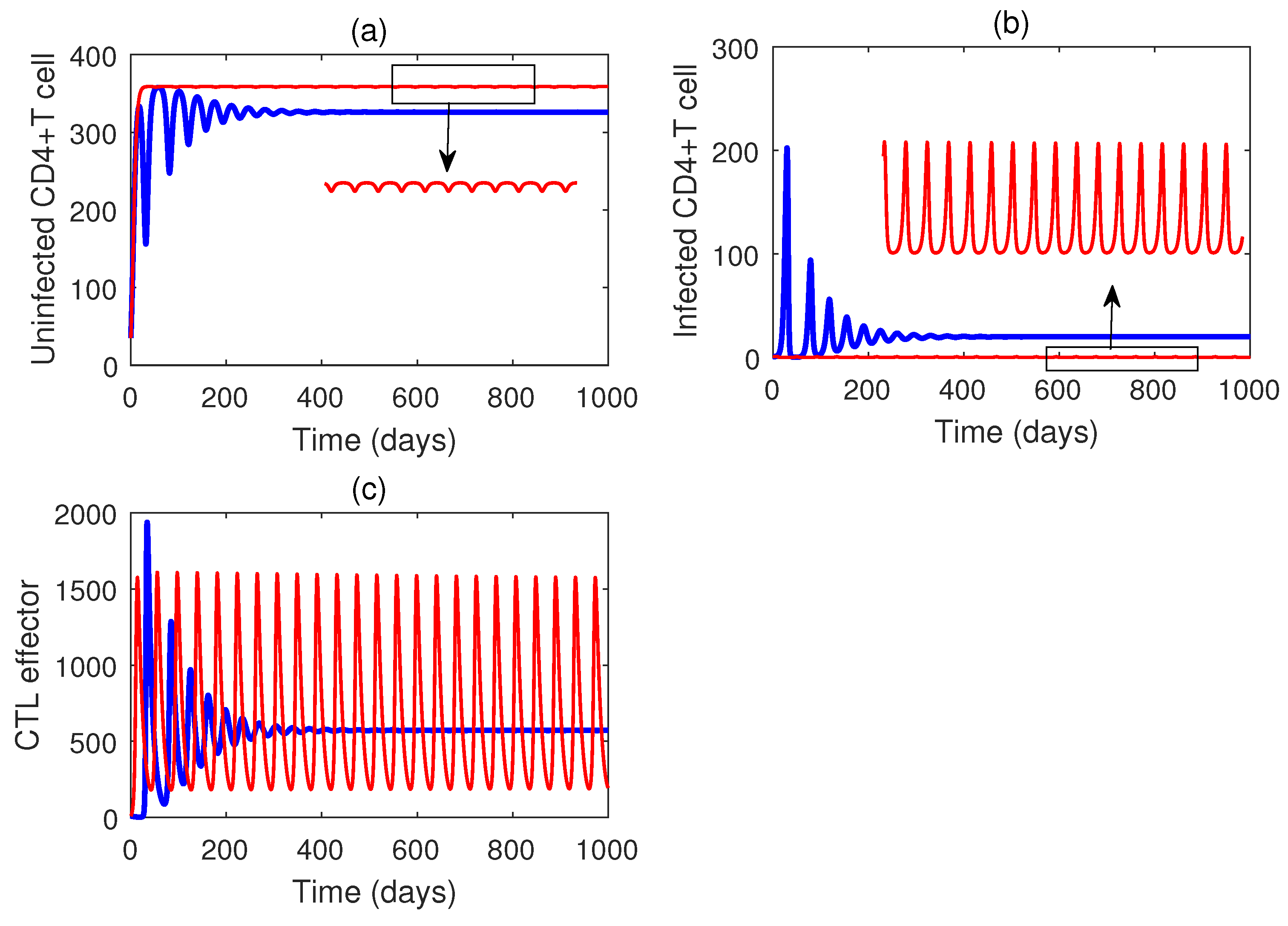
The time series solution of the system is plotted in Figure 2, taking the values of the model parameters from Table 1. It is observed that the coexistence equilibrium is asymptotically stable. The system moves towards the endemic equilibrium. This means the system is stable in nature.
Figure 2. (ac): Time series solution of the system (1) for the parameter values given in Table 2. The system is asymptotically stable around the endemic equilibrium  E EE . Red lines indicate  γ 2 = 0.6 , and blue curves represent  γ 2 = 0.0005 . Red lines indicate a periodic solution for  γ 2 = 0.6 .
Mathematics 14 01079 g002
Table 2. Parameter sets used in Figure 2, Figure 3, Figure 4, Figure 5, Figure 6, Figure 7, Figure 8, Figure 9 and Figure 10.
FiguresParameter Set
Figure 2 a = 12 , μ 1 = 0.1 , α = 0.00065 , η 1 = 0.0035 , η 2 = 0.8 β 1 = 0.00125
ϵ 1 = 0.3 , μ 2 = 0.12 , γ 1 = 0.0005 , γ 2 = 0.6 , μ 3 = 0.1 , ϵ 2 = 2 × 10 6
Figure 3Parameter set is the same as in Figure 2
Figure 4 a = 12 , μ 1 = 0.1 , α = 0.00065 , η 1 = 0.0035 , η 2 = 0.8 , ϵ 1 = 0.3 ,
μ 2 = 0.12 , γ 1 = 0.0005 , γ 2 = 0.2 , μ 3 = 0.1 , ϵ 2 = 2 × 10 6
Figure 5Parameter set is the same as in Figure 4
Figure 6
Figure 7 a = 10 ; μ 2 = 0.12 ; ϵ 1 = 0.02 ; η 1 = 0.25 ; α = 0.005
γ 1 = 0.005 , μ 3 = 0.1 , μ 1 = 0.1 , η 2 = 0.25 , ϵ 2 = 0.02
Figure 8 μ 2 = 0.12 , ϵ 1 = 0.02 , η 1 = 0.25 , α = 0.005 , γ 1 = 0.005 ,
μ 3 = 0.1 , μ 1 = 0.1 , η 2 = 0.25 , ϵ 2 = 0.02 , γ 2 = 0.006
Figure 9 a = 10 , δ = 0.001 , μ 1 = 0.001 , ϵ 1 = 0.0015 , ϵ 2 = 0.002 , η = 0.05 ,
α = 0.005 , γ 1 = 0.05 , μ 2 = 0.002 , γ 2 = 0.02 , μ 3 = 0.01
β = 0.0015 , A = 10.1 , B = 30.1 , R = 0.01 , S = 0.1
Figure 10Parameter set is the same as in Figure 10
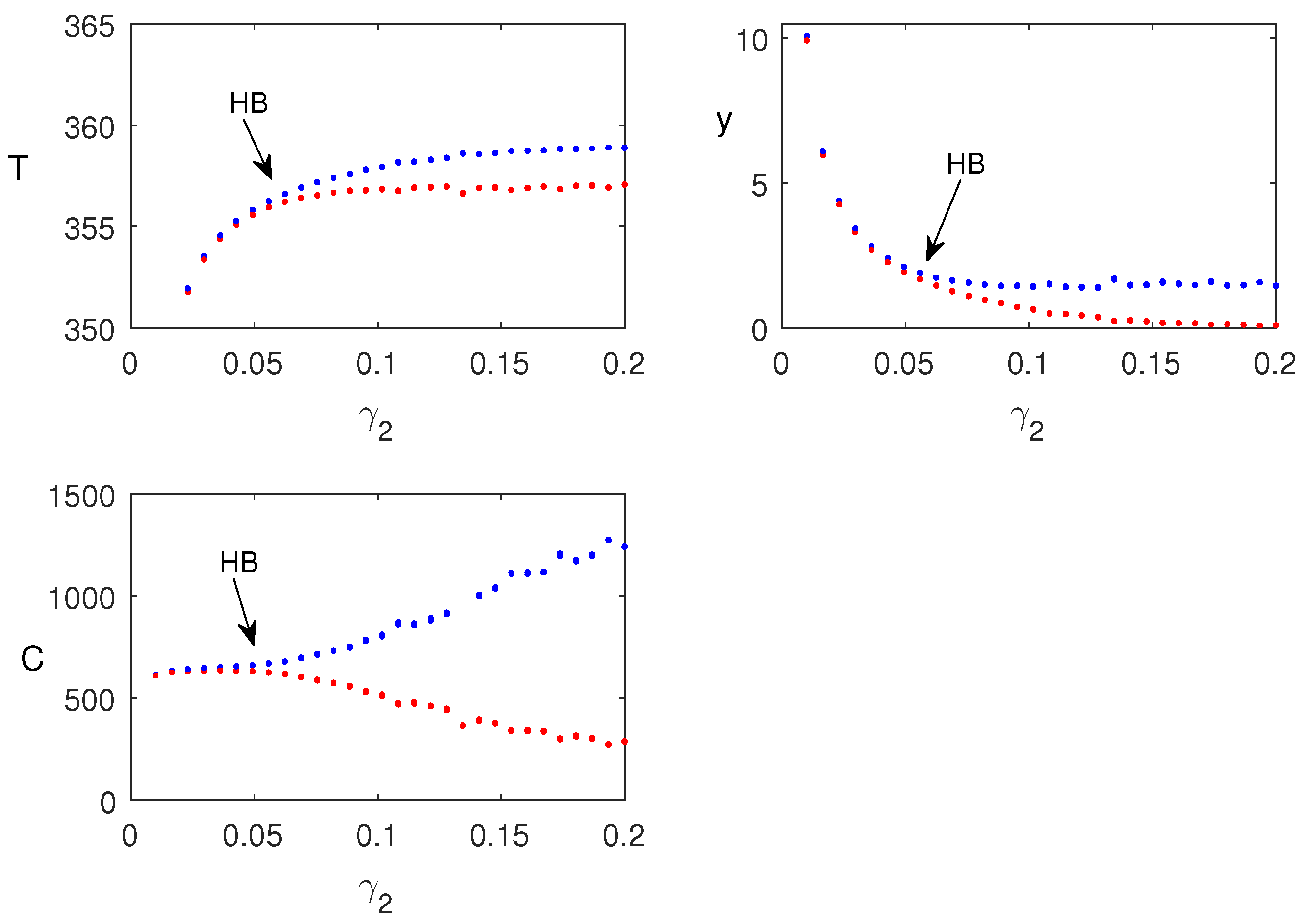
The bifurcation diagram of the system is shown in Figure 3 by varying  γ 2 . The system bifurcates into a periodic solution when  γ 2  passes the critical value,  γ 2 * = 0.0515  (approx.).
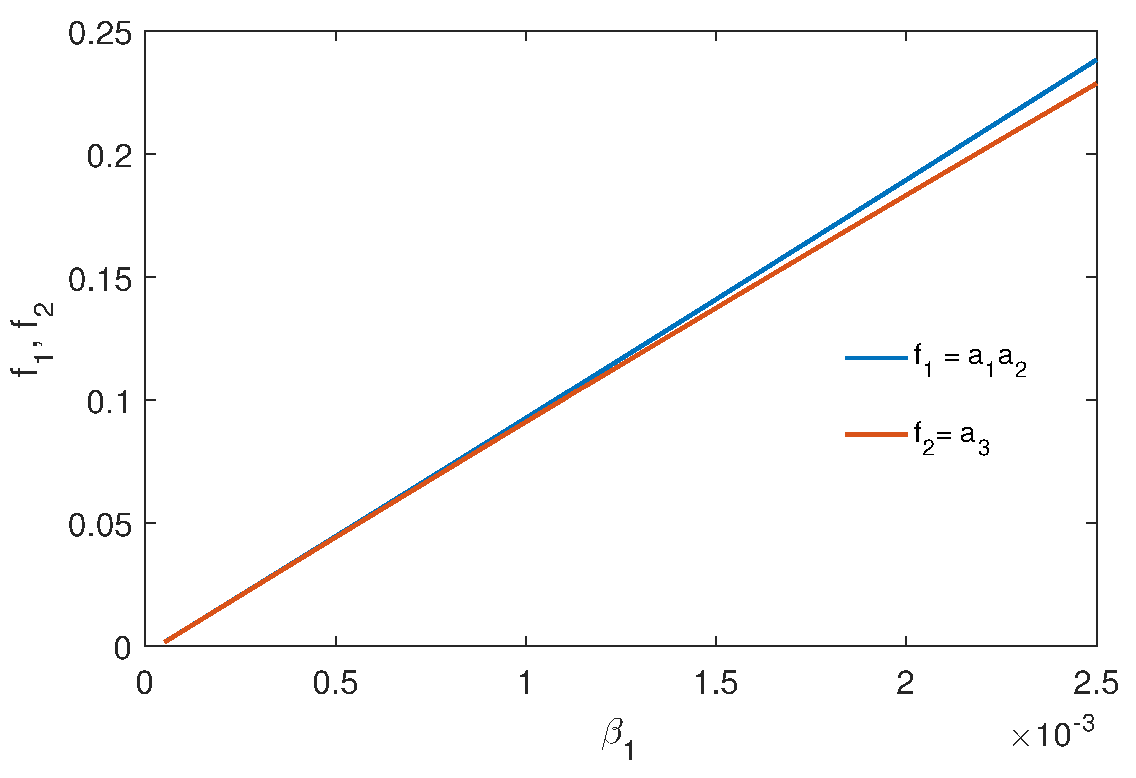
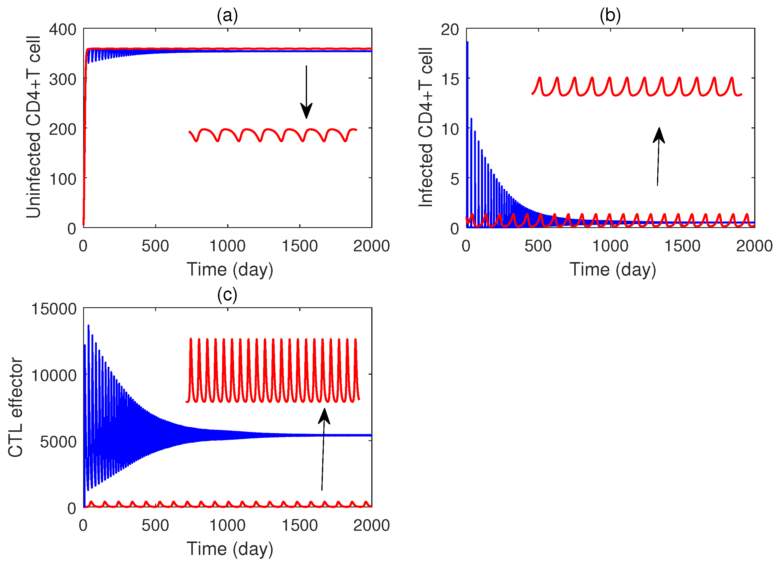
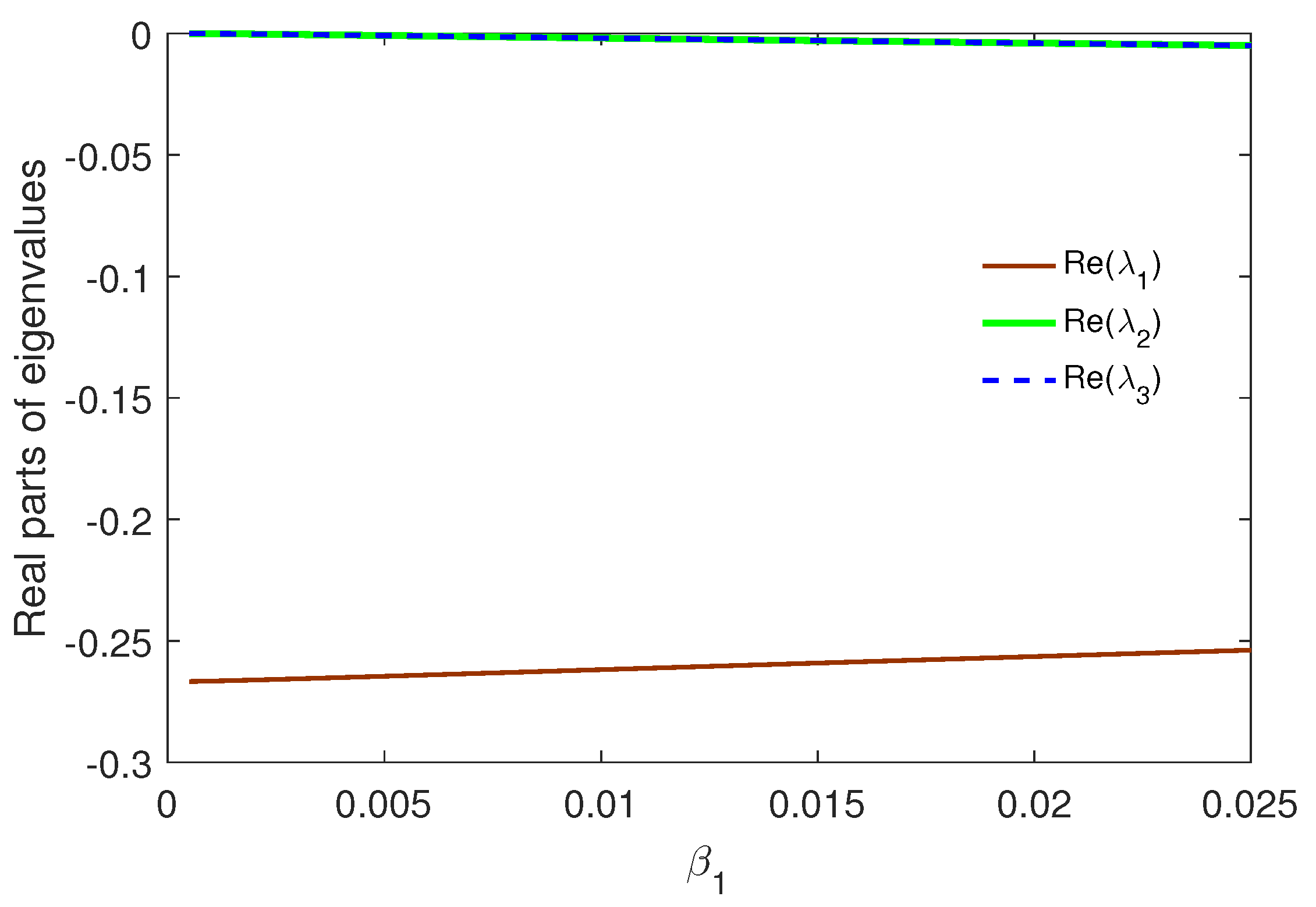
In Figure 4, the time series solutions are plotted for different values of the infection rate  β 1 . A bifurcating periodic solution is observed when the immune response rate is higher and the infection rate is lower, specifically at  β 1 = 0.005 . Furthermore, the conditions of Theorem 3 are verified numerically using Figure 5 and Figure 6. Figure 5 shows the real parts of the eigenvalues, where a pair of purely imaginary roots is observed when  β 1 < β 1 * = 0.007513 ( a p p r o x . ) . Moreover, Figure 6 confirms that the condition of Theorem 3,  a 1 a 2 a 3 = 0 , holds at  β 1 = β 1 * .
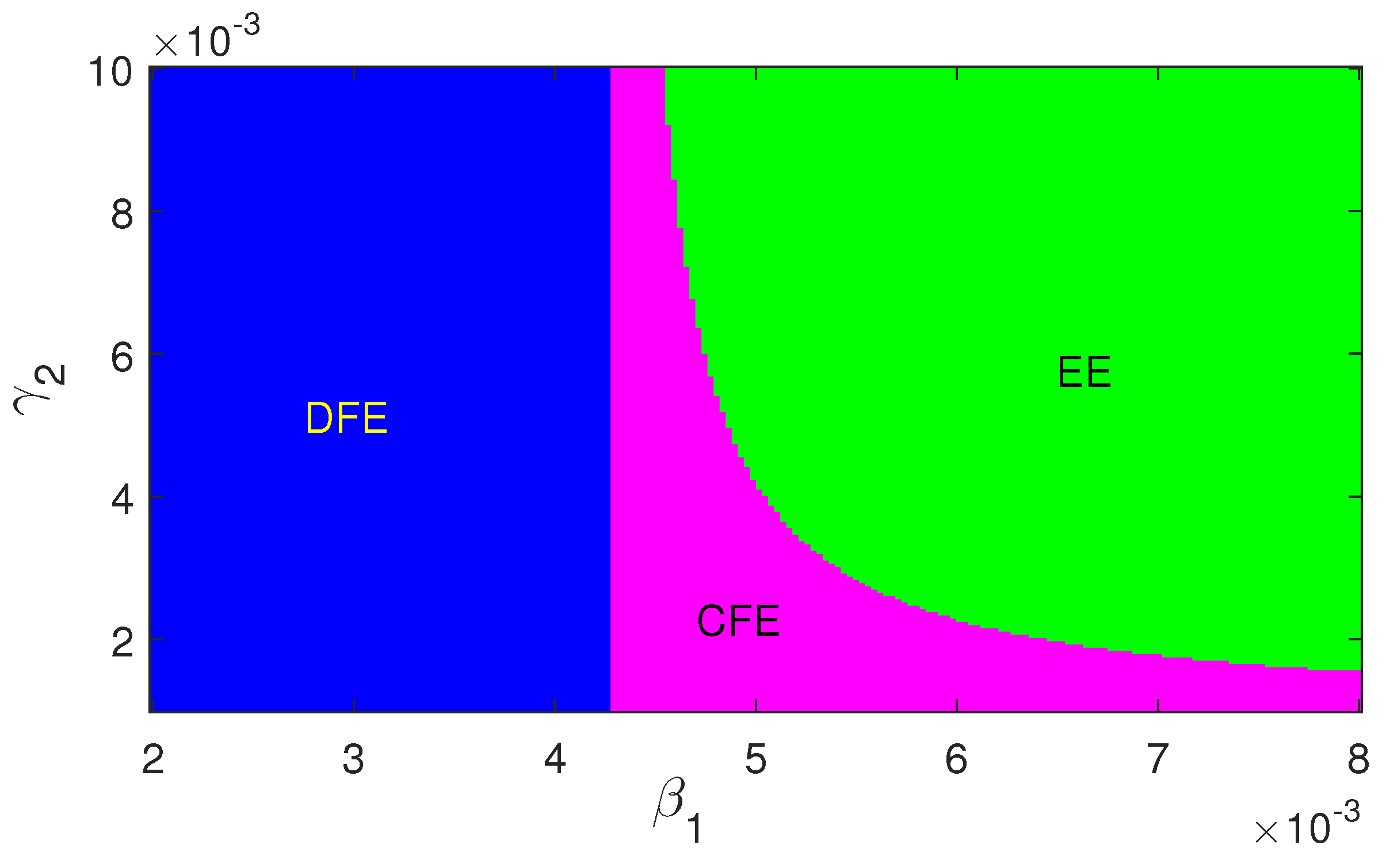
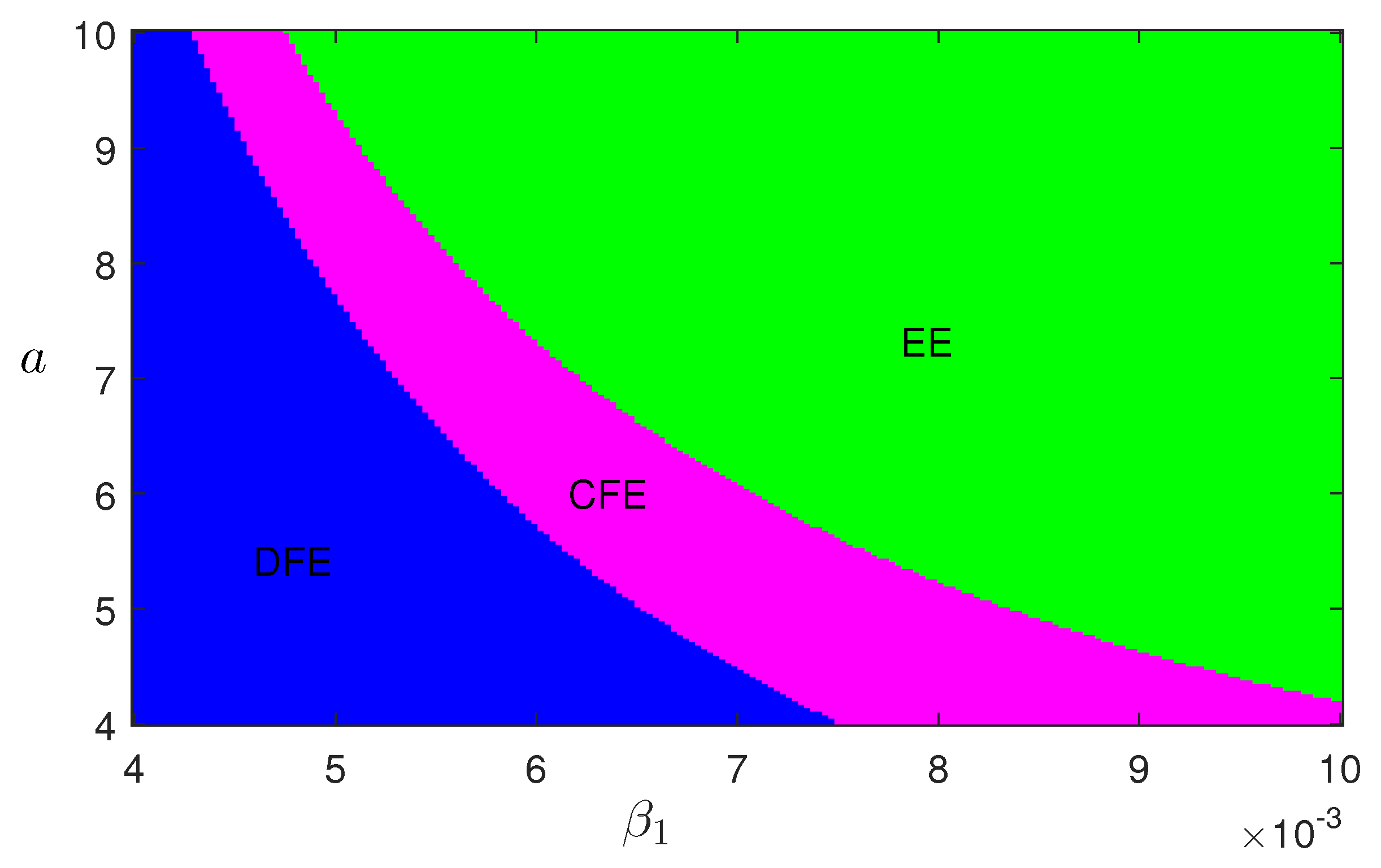
Regions of stability of the equilibrium points are plotted in Figure 7 and Figure 8. The figures show that for higher infection, the endemic equilibrium is feasible. The parameter set is given in Table 2. Figure 8 shows that the endemic is stable in nature for the set of parameters used for these figures. Also,  α  has a stabilizing role in the dynamics. A high rate of immune response  γ 2  can cause oscillation in the system when the infection rate is low, as shown in Figure 3. Thus, when we use immune activator drugs, we have to use proper doses. Optimal drug dosing can reduce the side effects.

6.2. Dynamics of the System with Optimal Control

The forward–backward sweep method is a widely used numerical technique for solving optimal control problems. It works by iteratively integrating the state equations forward in time with an initial guess for the controls and then integrating the adjoint (costate) equations backward in time using terminal conditions. At each iteration, the controls are updated point-wise according to the optimality conditions derived from the Hamiltonian, typically with bounds enforced. This forward–backward cycle is repeated until the state, adjoint, and control trajectories converge, yielding an approximate solution to the optimal control problem.
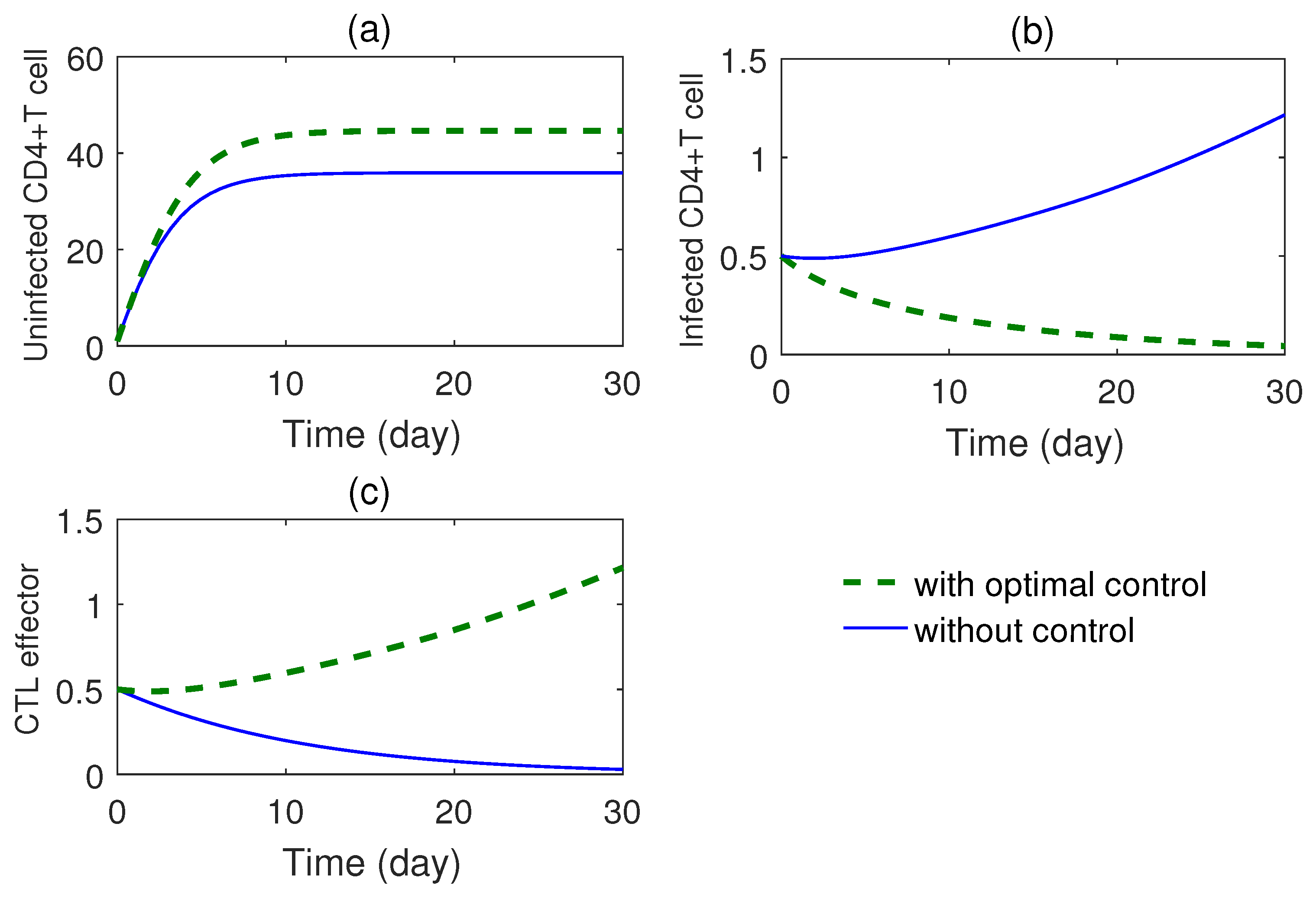
From optimal control studies (Figure 9 and Figure 10), several interesting results are obtained. The CTL effector population is found to decrease in all cases. Thus, an optimal control approach will help in designing an innovative, cost-effective, safe therapeutic regimen of HAART and IL-2, where the uninfected cell population will be enhanced with a simultaneous decrease in the infected cell population. Moreover, successful immune reconstitution can also be achieved with an increase in the precursor CTL population. Mathematical modeling of viral dynamics thus enables maximization of therapeutic outcomes even in the case of multiple therapies with the specific goal of reversal of immunity impairment.
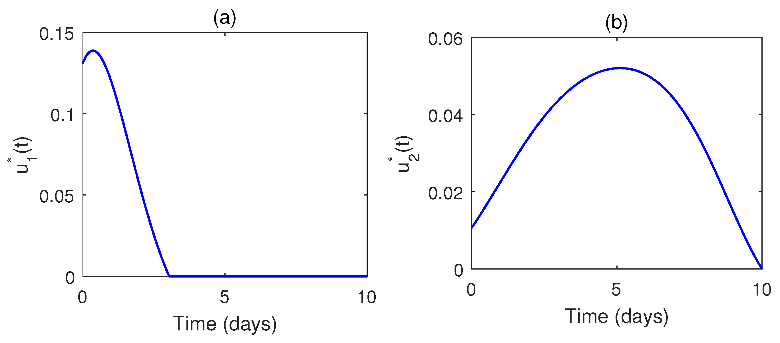
Figure 9 represents the control pair  u * ( t )  for the RTI drug for the parameter set as given in Table 1. The RTI drug is administered at nearly full level for approximately 20 days; after that, it is reduced to zero at 30 days. In Figure 10, we see that during the treatment period, the infected T cells increase almost linearly, and the CTL responses also increase, whereas the virus-producing cells linearly decrease.

6.3. PRCC Analysis for the Optimal System

To study the sensitivity of the optimal control system, the partial rank correlation coefficient (PRCC) with respect to y was computed as follows:
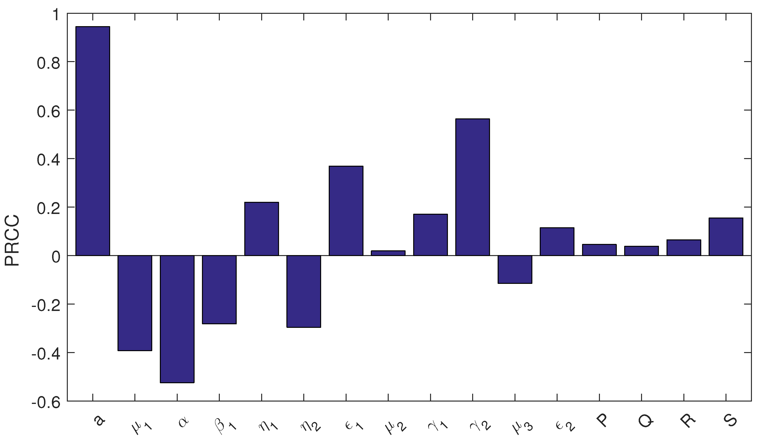
Parameters were sampled using Latin hypercube sampling (LHS). For each sample, the optimal system was solved numerically to obtain trajectories of  T ( t ) y ( t ) , and  C ( t ) . The number of uninfected CD4+ T cells,  T ( t ) , was chosen as the response variable. Both inputs and outputs were rank-transformed to reduce nonlinear effects. Partial rank correlation coefficients (PRCCs) were then calculated while controlling for other parameters. The PRCC values were plotted as bar graphs: positive values indicate parameters that increase the response, while negative values indicate parameters that decrease it. Figure 11 highlights the most influential parameters on system dynamics. We found that growth rate a, immune response  γ 2 , weight constants, and penalty multipliers show positive sensitivity to uninfected CD4+ T cells, whereas infection rate  β 1 , intra-population competition rate  α , etc. have a negative influence on uninfected CD4+ T cells, T.

7. Discussion and Conclusions

In this study, we derived a mathematical framework to elucidate the dynamics of the human immune system in response to HIV infection under the combined influence of highly active antiretroviral therapy (HAART) and interleukin-2 (IL-2). Biologically, HIV infection is characterized by the progressive depletion of CD4+ T lymphocytes, which compromises immune surveillance and predisposes patients to opportunistic infections. Our model captures these processes by incorporating viral replication, immune activation, and therapeutic intervention, thereby providing a quantitative lens through which the interplay of infection and treatment can be examined.
Analysis of the system revealed that stability and oscillatory behavior depend critically on the infection rate parameter  β 1  and immune response rate,  γ 2 . For certain values of these parameters, the immune system either stabilizes or destabilizes, reflecting biological scenarios of viral suppression or resurgence. Notably, bifurcating periodic solutions observed at  β 1 = 0.0035  correspond to oscillatory viral loads and T cell counts, a phenomenon consistent with clinical observations of viral blips during therapy. Using normal form theory, the bifurcating periodic solution is a subcritical type. Interestingly, these oscillatory immune responses parallel the immune dysregulation phenomena reported in vaccine-related studies such as Zhang et al. [54], Jia et al. [55], and Xu et al. [56], where aberrant immune activation and periodic manifestations were observed following COVID-19 vaccination. Such parallels reinforce the broader relevance of oscillatory immune dynamics across different immunological contexts.
From a control-theoretic perspective, we established the existence of optimal therapeutic strategies by applying the Pontryagin minimum principle. The derived adjoint equations and control laws formalize the biological trade-off between drug-induced viral suppression and immune stimulation. The resulting two-point boundary value problem (TPBVP) encapsulates the coupled dynamics of viral replication, immune recovery, and drug administration. Computationally, the forward–backward sweep method yielded dosing policies that balance pharmacological costs against immunological benefits, thereby reflecting the clinical objective of maximizing patient health while minimizing toxicity and expense. Also, the optimal control pair is unique for the optimal control problem formulated here.
Biologically, IL-2 serves as an immune activator that enhances the proliferation and survival of CD4+ T cells, while HAART suppresses viral replication by targeting reverse transcriptase and other viral enzymes. Our findings demonstrate that the synergistic application of these therapies not only improves the uninfected T cell population but also reduces the reservoir of infected cells. This dual effect translates into prolonged immune competence and extended patient survival. Importantly, the optimal control strategy was shown to reduce side effects and improve cost-effectiveness, aligning with clinical goals of sustainable long-term therapy.
In conclusion, the integration of mathematical modeling with biological interpretation underscores the potential of optimal control theory in designing effective HIV treatment regimens. The combination of HAART and IL-2, when administered under an optimized dosing policy, enhances immune recovery, suppresses viral persistence, and improves life expectancy in HIV-infected individuals. This framework provides a rigorous foundation for future quantitative investigations into combination therapies. Moreover, methodological advances such as those proposed by Cheng et al. [57] in stability analysis offer promising extensions to our bifurcation framework, potentially enabling deeper insights into the robustness of immune dynamics under therapeutic interventions. Collectively, these comparisons highlight the importance of mathematical biology in guiding clinical decision-making and situating HIV modeling within a broader landscape of immune regulation studies.

Author Contributions

Conceptualization, I.M.A. and F.A.B.; Methodology, I.M.A. and F.A.B.; Formal analysis, I.M.A. and F.A.B.; Investigation, I.M.A. and F.A.B.; Writing—original draft, I.M.A. and F.A.B.; Writing—review and editing, I.M.A. and F.A.B.; Visualization, I.M.A. and F.A.B. All authors have read and agreed to the published version of the manuscript.

Funding

This research received no external funding.

Data Availability Statement

The original contributions presented in this study are included in the article. Further inquiries can be directed to the corresponding authors.

Conflicts of Interest

The authors declare no conflicts of interest.

References

  1. Gillespie, S.L.; Chinen, J.; Paul, M.E.; Shearer, W.T. Human immunodeficiency virus infection and acquired immunodeficiency syndrome. In Clinical Immunology; Elsevier: Amsterdam, The Netherlands, 2019; pp. 545–560. [Google Scholar]
  2. Lazarus, J.V.; Wohl, D.A.; Cascio, M.; Guaraldi, G.; Rockstroh, J.; Hodson, M.; Richman, B.; Brown, G.; Anderson, J.; Fuster-RuizdeApodaca, M.J. Long-term success for people living with HIV: A framework to guide practice. HIV Med. 2023, 24, 8–19. [Google Scholar] [CrossRef] [Scilit]
  3. Landovitz, R.J.; Scott, H.; Deeks, S.G. Prevention, treatment and cure of HIV infection. Nat. Rev. Microbiol. 2023, 21, 657–670. [Google Scholar] [CrossRef] [Scilit]
  4. Eron, J.J.; Little, S.J.; Crofoot, G.; Cook, P.; Ruane, P.J.; Jayaweera, D.; VanderVeen, L.A.; DeJesus, E.; Zheng, Y.; Mills, A.; et al. Safety of teropavimab and zinlirvimab with lenacapavir once every 6 months for HIV treatment: A phase 1b, randomised, proof-of-concept study. Lancet HIV 2024, 11, e146–e155. [Google Scholar] [CrossRef] [Scilit]
  5. Laher, F.; Mahlangu, N.; Sibiya, M. Beliefs about HIV cure: A qualitative study of people living with HIV in Soweto, South Africa. S. Afr. J. HIV Med. 2025, 26, 1644. [Google Scholar]
  6. Okesanya, O.J.; Ayeni, R.A.; Amadin, P.; Ngwoke, I.; Amisu, B.O.; Ukoaka, B.M.; Ahmed, M.M.; Oso, T.A.; Musa, S.S.; Lucero-Prisno, D.E. Advances in HIV Treatment and Vaccine Development: Emerging Therapies and Breakthrough Strategies for Long-Term Control. AIDS Res. Treat. 2025, 2025, 6829446. [Google Scholar]
  7. Perelson, A.S.; Nelson, P.W. Mathematical analysis of HIV-1 dynamics in vivo. SIAM Rev. 1996, 39, 3–44. [Google Scholar] [CrossRef] [Scilit]
  8. Nowak, M.A.; May, R.M. Virus Dynamics: Mathematical Principles of Immunology and Virology; Oxford University Press: Oxford, UK, 2000. [Google Scholar]
  9. The INSIGHT–ESPRIT Study Group; SILCAAT Scientific Committee. Interleukin-2 therapy in patients with HIV infection. N. Engl. J. Med. 2009, 361, 1548–1559. [Google Scholar] [CrossRef] [Scilit] [PubMed]
  10. Li, C.; Sun, J.P.; Wang, N.; Yan, P.; Wang, R.; Su, B.; Zhang, T.; Wu, H.; Chen, H.; Li, Z.; et al. Plasma cytokine expression and immune reconstitution in early and delayed anti-hiv 96-weeks treatment: A retrospective study. AIDS Res. Hum. Retroviruses 2024, 40, 101–109. [Google Scholar] [CrossRef] [Scilit] [PubMed]
  11. Rasi, G.; Emili, E.; Conway, J.M.; Cotugno, N.; Palma, P. Mathematical modeling and mechanisms of HIV latency for personalized anti latency therapies. Npj Syst. Biol. Appl. 2025, 11, 64. [Google Scholar] [PubMed]
  12. D’Orso, I.; Forst, C.V. Mathematical models of HIV-1 dynamics, transcription, and latency. Viruses 2023, 15, 2119. [Google Scholar] [CrossRef] [Scilit]
  13. Tarasova, O.; Petrou, A.; Ivanov, S.M.; Geronikaki, A.; Poroikov, V. Viral factors in modulation of host immune response: A route to novel antiviral agents and new therapeutic approaches. Int. J. Mol. Sci. 2024, 25, 9408. [Google Scholar] [CrossRef] [Scilit]
  14. AlShamrani, N.H. A diffusion-based HIV model with inflammatory cytokines and adaptive immune impairment. Front. Appl. Math. Stat. 2025, 11, 1659816. [Google Scholar] [CrossRef] [Scilit]
  15. Li, Y.; Zhang, L.; Zhang, J.; Liu, S.; Peng, Z. Dynamical modeling and data analysis of HIV infection with infection-age, CTLs immune response and delayed antibody immune response. J. Math. Biol. 2025, 91, 57. [Google Scholar] [CrossRef] [Scilit]
  16. de Carvalho, J.P.S.M. Qualitative analysis of HAART effects on HIV and SARS-CoV-2 coinfection model. Appl. Math. 2025, 70, 495–516. [Google Scholar] [CrossRef] [Scilit]
  17. Alsulami, I.M. On the stability, chaos and bifurcation analysis of a discrete-time chemostat model using the piecewise constant argument method. AIMS Math. 2024, 9, 33861–33878. [Google Scholar] [CrossRef] [Scilit]
  18. Rathnayaka, N.S.; Wijerathna, J.K.; Pradeep, B.G.S.A. Stability Properties and Hopf Bifurcation of a Delayed HIV Dynamics Model with Saturation Functional Response, Absorption Effect and Cure Rate. Int. J. Anal. Appl. 2025, 23, 92. [Google Scholar] [CrossRef] [Scilit]
  19. Hmarrass, H.; Qesmi, R. Global Stability and Hopf Bifurcation of a Delayed HIV Model with Macrophages, CD4+ T Cells with Latent Reservoirs and Immune Response. Eur. Phys. J. Plus 2025, 140, 335. [Google Scholar] [CrossRef] [Scilit]
  20. Lan, R.Y.; Selmi, C.; Gershwin, M.E. The regulatory, inflammatory, and T cell programming roles of interleukin-2 (IL-2). J. Autoimmun. 2008, 31, 7–12. [Google Scholar] [CrossRef] [Scilit]
  21. Eggleton, J.S.; Nagalli, S. Highly active antiretroviral therapy (HAART). In StatPearls [Internet]; StatPearls Publishing: Orlando, FL, USA, 2023. [Google Scholar]
  22. Amendola, A.; Poccia, F.; Martini, F.; Gioia, C.; Galati, V.; Pierdominici, M.; Marziali, M.; Pandolfi, F.; Colizzi, V.; Piacentini, M.; et al. Decreased CD95 expression on naive T cells from HIV-infected persons undergoing highly active anti-retroviral therapy (HAART) and the influence of IL-2 low dose administration. Clin. Exp. Immunol. 2000, 120, 324–332. [Google Scholar]
  23. Abiodun, O.; Olukayode, A.; Ndako, J. Mathematical Modeling and Optimal Control Strategies of HIV/AIDS with HAART. In Proceedings of the 2023 International Conference on Science, Engineering and Business for Sustainable Development Goals (SEB-SDG), Omu-Aran, Nigeria, 5–7 April 2023. [Google Scholar]
  24. Gumel, A.B.; Zhang, X.W.; Shivakumar, P.N.; Garba, M.L.; Sahai, B.M. A New Mathematical Model for Assessing Therapeutic Strategies for HIV. J. Theor. Med. 2002, 4, 147–155. [Google Scholar]
  25. Pontryagin, L.S.; Boltyanskii, V.G.; Gamkrelidze, R.V.; Mishchenko, E.F. The Mathematical Theory of Optimal Processes; Classic Reference Introducing the Pontryagin Maximum Principle; Routledge: London, UK, 1962. [Google Scholar]
  26. Campos, C.; Silva, C.J.; Torres, D.F.M. Numerical Optimal Control of HIV Transmission in Octave/MATLAB. Mathematics 2019, 25, 1. [Google Scholar] [CrossRef] [Scilit]
  27. Boukary, O.; Malicki, Z.; Elisée, G. Mathematical Modeling and Optimal Control of an HIV/AIDS Transmission Model. Int. J. Anal. Appl. 2024, 22, 234. [Google Scholar] [CrossRef] [Scilit]
  28. Al Basir, F.; Nisar, K.S.; Alsulami, I.M.; Chatterjee, A.N. Dynamics and optimal control of an extended SIQR model with protected human class and public awareness. Eur. Phys. J. Plus 2025, 140, 152. [Google Scholar] [CrossRef] [Scilit]
  29. Musa, S.; John, S.; Salvation, H. Mathematical Modeling of HIV Transmission Dynamics: Incorporating Treatment and Removal as Control Strategies. Int. J. Sci. Res. 2025, 9, 16–31. [Google Scholar]
  30. Chazuka, Z.; Madubueze, C.E.; Mathebula, D. Modelling and analysis of an HIV model with control strategies and cost-effectiveness. Results Control Optim. 2024, 14, 100355. [Google Scholar]
  31. Rana, P.S.; Sharma, N.; Priyadarshi, A. Mathematical Modeling and Optimal Control of a Deterministic SHATR Model of HIV/AIDS with Possibility of Rehabilitation: A Dynamic Analysis. Tamkang J. Math. 2024, 55, 267–285. [Google Scholar] [CrossRef] [Scilit]
  32. Kumar, N.; Kashif, M.; Chauhan, T.S.; Chauhan, I.S. Modeling and Control of HIV/AIDS Epidemics: A Stochastic and Optimal Control Perspective. J. Nonlinear Math. Phys. 2025, 32, 80. [Google Scholar] [CrossRef] [Scilit]
  33. Alblowy, A.H.; Maan, N.; Ibrahim, A.A. Optimal control strategies for SGLT2 inhibitors as a novel anti-tumor agent and their effect on human breast cancer cells with the effect of time delay and hyperglycemia. Comput. Biol. Med. 2023, 166, 107552. [Google Scholar] [CrossRef] [Scilit]
  34. Teklu, S.W.; Terefe, B.B.; Mamo, D.K.; Abebaw, Y.F. Optimal control strategies on HIV/AIDS and pneumonia co-infection with mathematical modelling approach. J. Biol. Dyn. 2024, 18, 2288873. [Google Scholar] [CrossRef] [Scilit]
  35. Février, M.; Dorgham, K.; Rebollo, A. CD4+ T cell depletion in human immunodeficiency virus (HIV) infection: Role of apoptosis. Viruses 2011, 3, 586. [Google Scholar] [CrossRef] [Scilit]
  36. Yates, A.; Stark, J.; Klein, N.; Antia, R.; Callard, R. Understanding the slow depletion of memory CD4+ T cells in HIV infection. PLoS Med. 2007, 4, e177. [Google Scholar]
  37. Boshier, F.A.T.; Reeves, D.B.; Duke, E.R.; Swan, D.A.; Prlic, M.; Cardozo-Ojeda, E.F.; Schiffer, J.T. Substantial uneven proliferation of CD4+ T cells during recovery from acute HIV infection is sufficient to explain the observed expanded clones in the HIV reservoir. J. Virus Erad. 2022, 8, 100091. [Google Scholar]
  38. Nath, B.J.; Sadri, K.; Sarmah, H.K.; Hosseini, K. An optimal combination of antiretroviral treatment and immunotherapy for controlling HIV infection. Math. Comput. Simul. 2024, 217, 226–243. [Google Scholar]
  39. Roy, P.K.; Chowdhury, S.; Chatterjee, A.; Majee, S.B. Mathematical Modeling of IL-2 Based Immune Therapy on T cell homeostasis in HIV; InTech: Toyama, Japan, 2012. [Google Scholar]
  40. Barish, S.; Ochs, M.F.; Sontag, E.D.; Gevertz, J.L. Evaluating optimal therapy robustness by virtual expansion of a sample population, with a case study in cancer immunotherapy. Proc. Natl. Acad. Sci. USA 2017, 114, E6277–E6286. [Google Scholar]
  41. Nath, B.J.; Sarmah, H.K.; Maurer, H. An optimal control strategy for antiretroviral treatment of HIV infection in presence of immunotherapy. Qual. Theory Dyn. Syst. 2022, 21, 30. [Google Scholar] [CrossRef] [Scilit]
  42. Culshaw, R.; Ruan, S. A delay-differential equation model of HIV-1 infection of CD4+ T-cells. Math. Biosci. 2000, 165, 425–444. [Google Scholar] [CrossRef] [Scilit] [PubMed]
  43. Wodarz, D.; Nowak, M. Specific therapy regimes could lead to long term immunological control to HIV. Proc. Natl. Acad. Sci. USA 1999, 96, 14464–14469. [Google Scholar]
  44. Teschl, G. Ordinary Differential Equations and Dynamical Systems; Graduate Studies in Mathematics; American Mathematical Society: Providence, RI, USA, 2012; Volume 140. [Google Scholar]
  45. Seifert, C.; Waurick, M. Evolutionary Equations: Picard’s Theorem for Partial Differential Equations, and Applications; Operator Theory: Advances and Applications; Birkhäuser: Basel, Switzerland, 2022; Volume 287. [Google Scholar]
  46. Brikhoff, G.; Rota, G. Ordinary Differential Equations; Ginn: Boston, MA, USA, 1982. [Google Scholar]
  47. Diekmann, O.; Heesterbeek, J.A.P.; Roberts, M.G. The construction of next-generation matrices for compartmental epidemic models. J. R. Soc. Interface 2010, 7, 873–885. [Google Scholar] [PubMed]
  48. Van den Driessche, P.; Watmough, J. Further notes on the basic reproduction number. In Mathematical Epidemiology; Springer: Berlin/Heidelberg, Germany, 2008; pp. 159–178. [Google Scholar]
  49. Diekmann, O.; Heesterbeek, J.A.P.; Metz, J.A. On the definition and the computation of the basic reproduction ratio R0 in models for infectious diseases in heterogeneous populations. J. Math. Biol. 1990, 28, 365–382. [Google Scholar] [CrossRef] [Scilit] [PubMed]
  50. Van den Driessche, P.; Watmough, J. Reproduction numbers and sub-threshold endemic equilibria for compartmental models of disease transmission. Math. Biosci. 2002, 180, 29–48. [Google Scholar] [CrossRef] [Scilit]
  51. Hassard, B.D.; Kazarinoff, N.D.; Wan, Y.H. Theory and Applications of Hopf Bifurcation; Cambridge University Press: Cambridge, UK, 1981. [Google Scholar]
  52. Fleming, W.H.; Rishel, R.W. Deterministic and Stochastic Optimal Control; Applications of Mathematics; Springer: New York, NY, USA, 1975; Volume 1. [Google Scholar] [CrossRef] [Scilit]
  53. Roy, P.K.; Nandi, S.; Ghosh, M.K. Modeling of a control induced system for product formation in enzyme kinetics. J. Math. Chem. 2013, 51, 2704–2717. [Google Scholar] [CrossRef] [Scilit]
  54. Zhang, H.Q.; Cao, B.Z.; Cao, Q.T.; Hun, M.; Cao, L.; Zhao, M.Y. An analysis of reported cases of hemophagocytic lymphohistiocytosis (HLH) after COVID-19 vaccination. Hum. Vaccines Immunother. 2023, 19, 2263229. [Google Scholar] [CrossRef] [Scilit] [PubMed]
  55. Jia, Y.; Fu, B.; Dong, L.; Zhao, M. Sweet syndrome induced by SARS-CoV-2 vaccines: A systematic review of patient-report studies. Hum. Vaccines Immunother. 2023, 19, 2217076. [Google Scholar] [CrossRef] [Scilit]
  56. Xu, K.; Gao, B.; Li, J.; Xiang, Y.; Cao, L.; Zhao, M. Clinical features, diagnosis, and management of COVID-19 vaccine-associated Vogt-Koyanagi-Harada disease. Hum. Vaccines Immunother. 2023, 19, 2220630. [Google Scholar] [CrossRef] [Scilit]
  57. Cheng, N.; Wang, W.; Zeng, H.; Liu, X.; Zhang, X. Novel exponential-weighted integral inequality for exponential stability analysis of time-varying delay systems. Appl. Math. Lett. 2026, 172, 109730. [Google Scholar] [CrossRef] [Scilit]
Figure 1. Diagram visually representing the interactions and processes described in the model (1), including the effects of HAART and IL-2.
Mathematics 14 01079 g001
Figure 3. Hopf bifurcation diagram of the system by varying  γ 2 . The system bifurcated into a periodic solution when  γ 2  crosses the critical value  γ 2 * = 0.0515 .  Here, we have plotted the maximum (blue dotted line) and minimum values (red dotted line) of the periodic solutions.
Mathematics 14 01079 g003
Figure 4. (ac): Behavior of the system (1) for  β 1 = 0.005  (red lines),  β 1 = 0.008  (blue lines), and other parameters given in Table 2.
Mathematics 14 01079 g004
Figure 5. Verifying the nature of eigenvalues for the existence of a Hopf bifurcation.  β 1  is varied, and the rest of the parameters are the same as in Figure 3.
Mathematics 14 01079 g005
Figure 6. Numerical verification of Hopf bifurcation (Theorem 3) taking  β 1  as the main parameter. Other parameter values are taken from Figure 3.
Mathematics 14 01079 g006
Figure 7. Region of stability of different equilibria plotted in  β 1 γ 2  space.
Mathematics 14 01079 g007
Figure 8. Region of stability of different equilibria plotted in  β 1 α  space.
Mathematics 14 01079 g008
Figure 9. (ac): Solution of the optimal system using parameter values in Table 1.
Mathematics 14 01079 g009
Figure 10. (a,b): Optimal profile for the two drugs plotted as a function of time. Parameter values are the same as in Figure 9.
Mathematics 14 01079 g010
Figure 11. Sensitivity analysis (PRCC analysis) of the parameters of the optimal system with respect to the uninfected CD4+ T cell, T.
Mathematics 14 01079 g011
Table 1. List of parameters used for numerical simulations [8,42,43].
ParameterDefinitionValue (Unit)
aconstant rate of production of  C D 4 + T  Cells15 cells day−1
μ 1 death rate of Uninfected  C D 4 + T  cells0.1 cells day−1
β 1 rate of infection0.00025–0.5 cells day−1
μ 2 death rate of infected cells0.2 cells/day
γ 1 clearance rate of infected cells by CTL0.002 day−1
γ 2 rate of proliferation of CTL0.02–0.6 day−1
μ 3 decay rate of CTL0.1 day−1
α intra-population competition0.00065 day−1
ϵ 1 activation rate of uninfected CD4+T cell by IL-20.005 day−1
ϵ 2 activation rate of CTL by IL-20.02 day−1
Disclaimer/Publisher’s Note: The statements, opinions and data contained in all publications are solely those of the individual author(s) and contributor(s) and not of MDPI and/or the editor(s). MDPI and/or the editor(s) disclaim responsibility for any injury to people or property resulting from any ideas, methods, instructions or products referred to in the content.