Article

Comparison of Analytical and Numerical Simulations for Underwater Ice Evolution and Nonlinear Dynamics of False Bottoms

by
Irina Nizovtseva
1,2,*,† and
Vladimir Ankudinov
3,4,†
1
Otto-Schott-Institut fur Materialforschung, Friedrich-Schiller University of Jena, 07743 Jena, Germany
2
Laboratory of Multiphase Physical and Biological Media Modeling, Ural Federal University, 620000 Yekaterinburg, Russia
3
Institute of Laser and Welding Technologies, State Marine Technical University, 198095 Saint Petersburg, Russia
4
Theoretical Department, Vereshchagin Institute for High Pressure Physics, Russian Academy of Sciences, Troitsk, 108840 Moscow, Russia
*
Author to whom correspondence should be addressed.
These authors contributed equally to this work.
Mathematics 2026, 14(6), 1040; https://doi.org/10.3390/math14061040
Submission received: 3 February 2026 / Revised: 5 March 2026 / Accepted: 17 March 2026 / Published: 19 March 2026

Abstract

In the present work, a comparative study of a model of the nonlinear solidification of a binary melt in the presence of a quasi-equilibrium mushy region and a binary phase field model of an aqueous solution of NaCl in water is performed. Nonlinear model is solved analytically in integral form with the effective coefficients of heat and mass transfer. Temperature and concentration distributions in the mushy zone are interpolated in the consideration of quasi-stationery boundary propagation. The binary phase field model introduces the temperature- and concentration-dependent mobility coefficients and allows the simultaneous solution of heat and solute transfer. The quantitative agreement between the analytical nonlinear model solved in integral form and the phase field model is shown. The applicability of the methods and details of the numerical implementation are discussed.
MSC:
35R35; 80A22; 74A15

1. Introduction

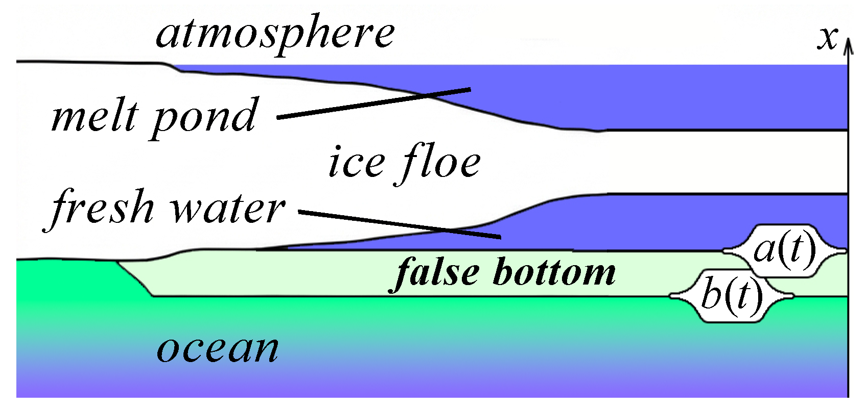
False bottoms, submerged ice layers that may form beneath summer sea ice at the interface between fresh meltwater and saline ocean water, provide a striking example of how small-scale phase-transition physics can affect large-scale ice–ocean exchange (Figure 1). From the mathematical modeling perspective, false-bottom evolution is a coupled nonlinear solidification problem with moving boundaries. In the present paper we analyze this dynamic using two complementary descriptions: a quasi-equilibrium mushy-layer theory that permits an exact analytical solution in integral form for a two-interface case, and a binary phase-field model that enables fully coupled numerical simulations with the heat transfer problem and solute concentration redistribution.

1.1. Physical Motivation for the Mathematical Model

The formation of ocean ice is of fundamental importance in physics and climate science, yet it remains challenging to model because of its nonlinearity and multiscale complexity. Late 19th century explorations and studies highlighted how sea-ice growth influences heat exchange between ocean and atmosphere; in 1889, Stefan formulated the classical moving-boundary phase-change problem (the Stefan problem), providing an early theoretical framework for solidification dynamics [3]. Subsequent climate analyses showed that a significant fraction of the Earth’s surface heat flux, on the order of 50% in high-latitude oceans, comes from the latent heat released during seawater freezing [4].
By the mid-20th century, solidification theory had expanded beyond Stefan’s single-phase model to address binary systems, e.g., saltwater or alloys; Scheil introduced analytical descriptions of solute partitioning during alloy solidification [5] with a mushy region (a porous two-phase zone of dendritic ice crystals bathed in brine), which forms when a liquid freezes non-isothermally. The development of casting technology extended the understanding of solidification velocity and solute diffusion and their impact on microstructures [6].
In parallel, advances in continuum mechanics led to treating mushy zones as continuum porous media, an approach later applied to sea-ice layers [7]. Thermodynamically consistent mushy-zone models were proposed in [8], enforcing coupled energy and salt conservation while respecting phase-equilibrium constraints. Fowler in 1985 explained the formation of chimneys or “freckles” in solidifying binary alloys via buoyancy-driven flow in the mush [9], emphasizing that even in diffusive regimes, fluid dynamics can induce channeling. The dynamics of binary solidification by solidifying aqueous solutions in the lab experiments show that a thin mushy layer can propagate with complex feedback between heat and salt diffusion [10], while the analytical solutions were provided in [11] for one-dimensional solidification.
By the last decade of the 20th century, the review of convection in mushy layers [12] unified knowledge from metallurgy, cryology, and fluid dynamics, and grounding common principles governing solidification patterns in metal castings and sea ice. Feltham et al. (2006) noted that sea ice is effectively a mushy layer, a reactive porous medium of ice and brine, and they used mushy-layer theory to model its thermodynamic behavior [13]. This historical evolution finally led to the discussion on the underwater ice growth phenomenon known as “false bottoms” which are thin ice plates forming below a melting ice floe, at the interface between cold, dilute meltwater and warmer seawater; see Figure 1.

1.2. False-Bottom Problem

The false-bottom structures have been a subject of intrigue since early polar expeditions. Anecdotal reports in the 1950s hinted at ice forming under summer melt pools, puzzling researchers at the time. Systematic observations during the AIDJEX program (Arctic Ice Dynamics Joint Experiment) provided some of the first documentation. In [14] it was reported “new ice” layers growing beneath Arctic pack ice in summer and autumn, which they attributed to freshwater from surface melt draining through the ice and refreezing underneath. In the 1960s, field measurements [15] confirmed that a significant fraction of meltwater can indeed escape the surface and accumulate below the ice; he observed fresh ice accretions in mass-balance studies of pack-ice floes, implicating subsurface refreezing in the summer ice budget. In [16], it was documented that there was a 20 cm yr 1 basal ice growth under the Ward Hunt Ice Shelf (Canada), (called “basement ice”) from fresh water lying beneath the shelf.
Controlled experiments and further field campaigns in the 1970s provided physical explanations for false bottoms. In [1], laboratory studies were conducted on under-ice melt ponds, reproducing the scenario of a fresh lens over seawater in an experimental tank. They observed rapid ice growth at the interface and identified the mechanism as a form of double-diffusive convection near the freezing point: the fresh water (lighter and at the freezing temperature) sits atop denser, slightly warmer salt water, leading to a convectively unstable interface. Cold fresh water descends and salt diffuses upward, effectively transferring heat downward and promoting freezing of the fresh layer and simultaneous melting at the bottom interface. Martin and Kauffman’s measurements of interface motion and temperature profiles confirmed a false bottom can thicken on the order of centimeters per day [1].
There is now strong evidence [17,18,19,20,21] that false bottoms form beneath summer sea ice and can significantly alter the structure and properties of the ice cover, e.g., by creating insulating voids or locally lifting the ice, thereby reducing the ocean heat flux to the original floe. The MOSAiC expedition (2019–2020) was the first to intentionally drift with sea ice for a full year, enabling detailed observations of summer processes such as under-ice meltwater layers and false-bottom formation [22]. During the MOSAiC summer phase, thin (0.1–1 m) freshwater layers persisted beneath melting ice for weeks, giving rise to false-bottom ice sheets at the interface with seawater. Drill-hole transects and ROV surveys indicated that these features were widespread, covering roughly 20% of the local under-ice area by late summer [23]. The presence of false bottoms altered the ice–ocean energy exchange by insulating the original ice, reducing ocean heat flux on the order of 5–10% [24].

1.3. Analytical Models

The formation of a false bottom involves a moving-boundary problem with two phase-change fronts: the upper interface, where fresh meltwater freezes onto the ice layer, and the lower interface, where the ice layer melts into the underlying seawater. Several studies have approximated similar two-front dynamics using sharp-interface models [25,26]. This approach has been applied successfully to the ice formation [27] and to the false-bottom dynamics [2] showing consistency with field observations [19]. The analytical solutions for mushy solidification problems make use of self-similar variables looking for an ansatz of the form ξ = z / α t (for some diffusivity α ), which implies that the characteristic thickness grows as α t .

1.4. Phase Field Methods

Originally developed for metallurgical microstructure simulation [28,29,30] based on the mean-field approach and on the Landau formalism introduced to the Allen–Cahn type of equation [31], phase-field (PF) models were applied to binary alloy solidification where mushy zones occur [30]. In PF the order parameter ϕ smoothly varies between ϕ = 1 in solids and ϕ = 0 in liquids. The evolution of ϕ is governed by partial differential equations derived from a thermodynamic potential, ensuring the interface motion arises naturally from free-energy minimization. Thermodynamic formulation of PF requires the total enthalpy and solute to be conserved [29,32], which is difficult to achieve in sharp-interface numerical models without manually imposing interface conditions.

1.5. Objectives and Scope of the Current Work

In the present work we perform a direct comparison between nonlinear analytical model of the formation of false bottom under ice floe in the summer [2] with the solution in integral form to the numerical solution of phase field model with temperature-dependent transport coefficients, solute redistribution and heat problem. The principal aim is a systematic cross-validation of two fundamentally different modeling paradigms, which are integral analytical mushy-layer theory and thermodynamically consistent phase-field simulations, under the same boundary conditions and parameter set.

2. The Nonlinear Analytical Model of “False Bottom” Evolution

In order to describe the nonlinear solidification dynamics of a false bottom, we employ a one-dimensional analytical model of the growing ice layer as a mushy zone of ice (solid phase) and sea water (liquid phase). This approach follows the quasi-equilibrium mushy-layer theory developed in prior works, e.g., Borisov’s model [33,34] and its extensions, solved analytically by Alexandrov et al. [25] for binary alloy solidification. There the exact solution was obtained for a unidirectional freezing problem with a mushy region, yielding explicit profiles for temperature, concentration, and solid fraction, as well as an algebraic relation for the solid fraction at the mush–solid interface.
Based on these points, we formulate the false-bottom problem with similar assumptions (as in [2,25]): (i) a quasi-steady temperature profile across the mushy zone; (ii) immediate local phase equilibration; and (iii) one-dimensional diffusive transport of heat and solute. A set of governing Equations (1)–(7) is provided below considering the conservation of energy and salt in the mushy layer and at its moving boundaries, followed by analytical solutions (8)–(14) that describe the evolution.
We specify the temperature and salinity fields inside the false bottom: under the quasi-equilibrium assumption, heat diffuses rapidly compared to the timescale of interface motion, so the temperature in the mushy layer can be approximated as linear in space at any given time. Accordingly, Equation (1) governs the evolution of salinity within the mushy zone (false bottom) by accounting for both diffusive transport and the effects of phase change:
τ [ ( 1 φ ) σ ] = ξ D σ ξ k σ φ τ , u s τ < ξ < u s τ + δ .
Here φ ( ξ , τ ) is the volume fraction of solid (ice) at position ξ and time τ within the mush, so ( 1 φ ) is the liquid fraction (brine porosity). Likewise σ ( ξ , τ ) is the salinity of the liquid in the pores (often taken nondimensionally, e.g., relative to the far-field salinity σ ). The left-hand side of Equation (1) represents the local rate of change of salt in the liquid portion of the mush. This changes due to two processes: (i) the diffusion of salt along the mushy layer, the first term on the right, and (ii) the redistribution of salt when liquid solidifies, the second term on the right). Physically, Equation (1) encapsulates constitutional freezing: as ice forms in the mush, salt is rejected or absorbed according to the partition ratio, and the excess salt diffuses away into the surrounding brine. This ensures salinity is redistributed within the mushy layer in step with ice crystallization. Equation (2) governs the temperature field θ in the mushy zone, assuming thermal diffusion is fast enough that the process is quasi-steady in time (no explicit θ / τ term):
ξ λ θ ξ + ρ L φ τ = 0 , u s τ < ξ < u s τ + δ .
Equation (3) imposes the phase equilibrium condition that couples the temperature and salinity in the two-phase region:
θ = θ 0 m σ , u s τ < ξ < u s τ + δ ,
where θ 0 is a reference freezing temperature (e.g., the melting point of pure water in the chosen units) and m is the liquidus slope (the rate at which the freezing point decreases with increasing salinity). This linear relation θ = θ m ( S ) (in dimensional terms) corresponds to the liquidus equation from the phase diagram T = T m ( S ) .
Equation (3) implies quasi-equilibrium assumption: the mushy zone is always at the phase boundary, with solid and liquid in thermodynamic equilibrium. Physically, this means that latent heat release has eliminated any thermal undercooling in the pores—the brine is as cold as it can be without freezing further. The temperature variable is eliminated from the mush equations: substituting the linear Equation (3) into Equation (2) effectively couples the heat and mass conservation laws into a single description.
The external thermal and solutal environment is defined with the Equation (4) in the far-field limit Equation (5):
θ s ξ = g s , ξ < u s τ ,
σ σ , ξ .
Far enough from the mushy zone the ocean salinity tends to σ , the ambient sea salinity, and the temperatures vary linearly with depth at fixed gradients g s and g . These serve as boundary conditions for solving the mushy-zone equations. We note that in Equation (4) diffusion in the solid ice is neglected which is a valid approximation since molecular salt diffusion in solid ice is practically zero, and the ice above is treated as a boundary with a fixed gradient rather than a time-evolving field, while in the phase-field model, diffusion in the solid phase is taken to be very small, but non-zero, in order to maintain continuity and numerical stability:
λ s g s λ θ ξ = ρ L ( 1 φ ) u s , ξ = u s τ ,
( 1 k ) ( 1 φ ) σ u s + D σ ξ = 0 , ξ = u s τ .
Equations (6) and (7) are written in the standard nondimensional quasi-equilibrium mushy-layer notation and are shown here to represent the structure of the energy and salt balances at the moving boundary ξ = u s τ . In the false-bottom setting, we apply analogous Stefan-type balances at each moving interface and rewrite them in dimensional variables using a ( t ) and b ( t ) and the mixture conductivity k i φ + k w ( 1 φ ) (see also Equations (11)–(14) below). The notational difference u s versus d a / d t reflects the quasi-stationary traveling-wave reduction (nearly constant interface speed over the considered interval) versus the time-dependent interface tracking used in the comparison. Finally, the latent-heat term is weighted by the phase fraction that actually undergoes phase change at the considered boundary (freezing of liquid into a mushy mixture vs. the solidification/melting of the residual liquid–solid within a mush). We also assume the convention is evaluated on the mushy side with the normal pointing from the mush, so the sign of the gradient is consistent throughout.
Under the above governing equations, one can obtain an exact analytical solution [2,35] for the steady growth of the false bottom in a diffusion-dominated regime. The solution assumes a quasi-stationary solidification: the mushy layer profiles attain a self-similar form moving with the interface velocities. In particular, the upper interface a ( t ) advances with a nearly constant speed u s , and the mushy zone reaches a steady thickness δ (or a slowly varying thickness that can be treated as approximately constant during early growth). These assumptions convert the partial differential system into an ODE boundary-value problem, which can be solved in closed form. Note that in the present paper we use these closed-form relations as the analytical reference for the comparison with the further PF simulations: a step-by-step reduction from the governing mushy-layer system to the integral relations is available in the primary derivations of the false-bottom theory and the underlying quasi-equilibrium mushy-layer solution as developed in [2,25].
The result is given by Equations (8)–(14) which describe the internal profiles of temperature, salinity, and solid fraction in the mush. We also keep in mind that while in (1)–(7) we follow the notation commonly used in the original quasi-equilibrium mushy-layer formulation, where, for example, θ denotes temperature and σ denotes salinity, starting from Equation (8) and throughout, we use the dimensional variables T and S for temperature and salinity, while the solute field in the PF model is denoted by the mass fraction c. Thus, the exact solution shows that the temperature in the mushy zone varies linearly with position between the two boundaries:
T m ( x , t ) = T a ( t ) ( x b ( t ) ) + T b ( t ) ( a ( t ) x ) a ( t ) b ( t ) .
Physically, a linear T-profile means there are no internal heat sources or sinks in the mush besides the phase change at the boundaries. In this case all latent heat release is balanced by conduction, resulting in a uniform gradient. By the equilibrium condition, T a and T b correspond to the liquidus temperatures of the interface salinities S a and S b respectively (see (10) below). Equation (8) thus provides an exact temperature profile across the false bottom, showing a smooth linear drop from the warmer upper interface a ( t ) to the colder lower interface b ( t ) , assuming T a > T b in typical scenarios.
Within the quasi-stationary self-similar reduction used to obtain the integral relations, the salinity solution yields an invariant: the product ( 1 φ ) S m becomes stationary in the reduced (moving-frame) description of the mushy layer [25], namely
t ( ( 1 φ ) S m ) = 0 , b ( t ) < x < a ( t ) .
Equation (9) should therefore be understood as a property of the quasi-stationary integral solution, steady in the moving frame, rather than as a general identity of the full time-dependent PDE system without these assumptions.
Physically, as the false bottom grows or evolves, the internal distribution of brine and solid adjusts such that the product of liquid fraction and salinity stays constant. If, for example, the solid fraction φ increases at some location, the liquid salinity S m there must drop proportionally to keep ( 1 φ ) S m fixed (the brine is being diluted exactly as pores fill with ice). This behavior is characteristic of self-similar solidification solutions. In practice, one can determine ( 1 φ ) S m as a function of x from the initial conditions or from integrating the steady-state form of Equation (1), and that profile then applies for all subsequent times until the assumptions break down.
Equation (10) restates the local equilibrium condition (3) in the dimensional variables of the solution,
T m ( x , t ) = m S m ( x , t ) , b ( t ) < x < a ( t )
We see that within the mushy layer, at any position x and time t, the temperature T m is exactly the freezing point corresponding to the local salinity S m . In this form, θ 0 from Equation (3) has been set to 0 by choosing the reference temperature as the melting point of pure ice so that T m = m S m ; one can always shift T by a constant without loss of generality. This equation emphasizes that the mush operates on the liquidus curve.
Equation (10) is used in practice to relate the interface temperatures and salinities, while the following (11) gives the rate of advance of the upper mush–ice interface, incorporating the effect of partial solid fraction at that boundary:
L V φ a d a d t = ( k i φ a + k w ( 1 φ a ) ) T m x .
The left side of Equation (11) represents the latent heat released per unit area per unit time as the interface moves, while the right-hand side represents the heat flux conducted away from the interface. Equation (11) therefore states that the latent heat released by freezing at the upper interface is carried off by thermal conduction into the surrounding material. It is a rearranged Stefan condition tailored to a mushy interface, compare to Equation (6) earlier. This equation yields the growth rate of the false-bottom’s top a ( t ) as a function of the prevailing heat flux: the stronger the thermal gradient into the cold ice above, the faster the freshwater freezes onto the false bottom. Furthermore
S a d a d t = D S m x
is the counterpart of Equation (7) in the final solution form (in dimensional variables). It equates the rate of salt advection by the moving interface to the diffusive salt flux at that interface.
Thus Equation (12) demands that any salt displaced by upward freezing is immediately diffused back into the mushy layer. In the limit that the upper interface is freezing pure water (initial freshwater lens) with S a 0 , the left side is nearly zero, which means there is no jump of salinity. Accordingly, the salinity gradient at the top of the mush a ( t ) adjusts to zero in that case. More generally, Equation (12) ensures a smooth salinity profile at the interface: it prevents a salinity discontinuity at x = a by expelling or absorbing salt via diffusion as the false bottom accretes fresh ice on top. This condition would be used together with Equation (11) to solve for the evolution of S a ( t ) and φ a ( t ) at the interface: it links the interface motion to the salinity gradient just below the interface, and thereby to the changing salinity of the pore brine at that boundary.
Equation (13) is the Stefan condition at the ice–ocean interface b ( t ) ; it balances the latent heat released by freezing with the heat fluxes at that boundary. The left-hand side here is the latent heat per unit area released as the mushy layer advances at velocity d a / d t , while the right-hand side represents the conductive heat flux out of the interface using the local mixture of ice and water with thermal conductivities k i and k w :
L V φ b d b d t = ( k i φ b + k w ( 1 φ b ) ) T m x + α h ρ w c w u ( T T b )
Here the last term is a standard bulk (Stanton-number type) parameterization of the turbulent ocean-side heat flux at the ice–ocean boundary: ρ w c w u sets the turbulent transport scale with u taken from the under-ice friction-velocity forcing used in the false-bottom datasets, while α h is a dimensionless transfer coefficient that lumps the unresolved boundary-layer physics into a single effective parameter. In this work we take α h = 0.0095 from the established parameter set used in the original false-bottom theory [2] based on AIDJEX/SHEBA data forcing in order to keep the analytical and PF comparisons under identical boundary exchange conditions.
Generally, one uses Equation (13) to find the rollback or advance rate of the lower interface b ( t ) given: a larger T (warmer ocean) or higher α h (more vigorous heat transfer) will increase the melting flux. Our analytical model’s inclusion of this convective term is a crucial adaptation for underwater ice formation—it further extends Alexandrov’s mushy-layer solution [2,35] by accounting for the finite heat flux from seawater.
The salt balance at the ice–ocean interface b ( t ) is given by
S b φ b d b d t = α s u ( S S b ) .
The left-hand side is the rate of salt pulling due to interface development (with S b the brine salinity at the interface and φ b the local solid fraction in the mushy zone). This is balanced by the convective salt flux, which carries away excess salt into the ocean, proportional to the flow velocity u and the salinity difference between the far-field water S and the interface brine S b .
To obtain the dynamics of the top a ( t ) and bottom b ( t ) boundary interfaces, we utilize the Alexandrov’s integral solution [2,35] with initial and boundary conditions defined with the experimental data on false bottom evolution taken from the AIDJEX and the SHEBA field experiments [19,36] (provided below in Section 3).

3. Phase Field Diffuse Interface Model of Water Solidification

In the present study, we use a one-dimensional phase-field (PF) model for an aqueous NaCl solution, formulated in terms of a solid–liquid order parameter φ ( x ) [ 0 , 1 ] ( φ = 0 liquid and φ = 1 solid), the solute mass-fraction field c ( x ) , and the temperature field T ( x ) . The free-energy density Equation (15) includes bulk and interfacial contributions and provides a temperature-dependent thermodynamic driving force for phase transformation, consistent with established PF formulations for binary systems [31,37] which is based on the thermodynamically consistent approach [38,39]. We consider the solid–liquid phase transition and latent heat release introduced with the heat capacity leap C p F T ( c , T ) dependent on the solute concentration and T [40,41]. The region of low solute concentrations of an aqueous NaCl solution (salinity of sea water S = 29.8 psu, which is equal to c = 2.98 wt% NaCl) has been investigated, and thus we neglect the chemical interaction contribution considering linear solidus and liquidus lines as well as the absence of additional chemical interactions in the liquid phase.
One can determine a complete PF free energy functional of a binary solution as
F ( ϕ , c , T ) = F 1 ( ϕ , c , T ) F 0 = V d V f ( ϕ , c , T ) + | γ ϕ ϕ | 2 2 + | γ c c | 2 2 .
Here one considers a certain deviation from the reference free energy F 0 , Equation (15), where V is the volume of the domain, γ ϕ is the gradient energy coefficient related to the solid–liquid interface energy, and γ c is the coefficient which defines the length scales of the compositional boundary [31,39]. Here the concentration c is treated as a mass fraction ( 0 c 1 ), which corresponds to 0–100 wt% NaCl; in particular, c = 0 denotes fresh water.
We consider only the slow phase-transitions and so the contributions of the non-equilibrium terms, such as first- and second-order fluxes of the order parameter, are vastly small. We extend and modify existing PF models [37,38,39,40] to properly account for the realistic Gibbs energies in the presence of a small temperature gradient.
The equilibrium contribution of the free energy density f ( ϕ , c , T ) could be written as
f ( ϕ , c , T ) = ( 1 c ) f A ( ϕ , T ) + c f B ( ϕ , T ) + R T ( 1 c ) ln ( 1 c ) + c ln c + c ( 1 c ) p ( ϕ ) M S ( c , T ) + ( 1 p ( ϕ ) ) M L ( c , T ) ,
where the separate contributions f A and f B are obtained from a thermodynamic database and are related to the free energy in Equation (16) by the limiting cases: f S ( c , T ) = f ( ϕ = 1 ; c ; T ) for the solid, and f L ( c , T ) = f ( ϕ = 0 ; c ; T ) for the liquid phase. Here f A corresponds to the fresh water, and f B is the saline composition at the eutectic point ( T e = 252 K, c e = 0.24 wt%):
f A ( ϕ , T ) = ( 1 p ( ϕ ) ) G H 2 O l i q u i d ( T ) + p ( ϕ ) G H 2 O c r y s t a l ( T ) + W g ( ϕ ) ; f B ( ϕ , T ) = ( 1 p ( ϕ ) ) [ G H 2 O l i q u i d ( T ) ( 1 c e ) + G N a C l a q . s o l . ( T ) c e ] +
p ( ϕ ) [ G H 2 0 c r y s t a l ( T ) ( 1 c e ) + G N a C l · 2 H 2 O c r y s t a l ( T ) c e ] + W g ( ϕ ) .
This form includes the Gibbs energies of liquid phase G H 2 O l i q u i d , which were implemented as a temperature-dependent Gibbs energy contributions, aqueous solutions of NaCl ions G N a C l a q . s o l . , and the ice G N a C l · 2 H 2 O c r y s t a l (see phase diagram and Gibbs energy coefficients for the NaCl + H2O system in [42]).
The function p ( ϕ ) is a phenomenological interpolation function with values p ( ϕ ϕ L = 0 ) = 0 and p ( ϕ ϕ S = 1 ) = 1 [38,39]. The g ( ϕ ) function is a wall of a simple double-well potential [31,37,39]:
p ( ϕ ) = ϕ 2 ( 3 2 ϕ ) ; g ( ϕ ) = ϕ 2 ( 1 ϕ ) 2 .
For the eutectic diluted aqueous solution one can assume the liquid phase to be ideal, which leads to M L = 0 in Equation (16). However, the description of the non-ideal mixture in the region of the higher concentration can be improved with the Redlich–Kister expansion with relevant coefficients [43]. A non-ideal solid is described using the empirical form of M S as [31,37]:
M S ( c , T ) = ( a 1 T a 2 ) ( 2 c 1 ) ( a 3 T + a 4 ) ,
where specific values of the constants a 1 a 4 are to be determined from thermodynamic conditions in the eutectic point. Specific values of coefficients a 1 , a 2 , a 3 , a 4 might be obtained from the conditions on the free energies at the eutectic point T = T e u t e c t i c , c = c e u t e c t i c , such as f L = f S , μ L = μ S and a common tangent construction (values are represented in Table 1).
A stable evolution of the entire system is given by the Lyapunov condition of a non-positive change of the total free energy Equation (15) in time from which one can obtain a dynamical equation as a functional derivative separately for conserved c and non-conserved ϕ order parameters [31,39]:
1 D ϕ ϕ t = δ F δ ϕ ; c t = · D c ( c ) δ F δ c ; T t = · k ( T ) C p ( c , T ) ρ ( T ) T .
Coupling PF with the heat transfer equation was provided with the introduction of the temperature variable T into PF model. At the same time, a response of the thermophysical properties is retrieved from the consideration of the phase transition as a finite leap of the heat capacity C p ( c , T ) [40,41]:
C p ( c , T ) = C p ( T ) + L v ( c ) σ C p 2 π exp ( T + m c ) 2 2 σ C p 2 ,
where composition-dependent melting temperature T m = m c followed from the liquidus slope m and current concentration; the smoothing coefficient σ C p = ( T m 273.15 ) / 10 Δ T 0.1 °C describes the width of the heat capacity leap associated with the latent heat of fusion. This implementation is based on the normalization of the finite leap on the enthalpy of fusion L v ( c ) . Such a leap describes the finite width of the liquidus–solidus range and allows one to introduce the mushy zone. The method with an effective heat capacity coefficient accounting C p ( T ) for the phase transition has proven effective for the modeling of the wide spectra of the heat transfer problems with high- and low-temperature gradients [40,41,44].
The concentration diffusion between solid and liquid phases has been introduced as a phase-dependent diffusion coefficient D c ( ϕ ) as a tanh-like step from D c ( ϕ = 0 ) = D c L to D c ( ϕ = 1 ) = D c S . In the present model we consider a temperature-dependent heat diffusivity k ( T ) , heat capacity C p ( T ) and density ρ ( T ) for a fixed composition of c [42]. The latent enthalpy of fusion of the composition of phases is defined as a linear mixture of H A and H B .
Numerical simulations were performed with the same boundary conditions as stated for analytical model Equations (13) and (14) with the constants (Table 1) and thermophysical properties obtained from thermodynamical data [42]. The single-dimensional task was prepared with a mesh size of = 0.1 mm for a domain with a length of 1 m. The presented task was solved using finite element method with the PARDISO direct solver in COMSOL Multiphysics 6.0 software [45] with the adaptive step for time integration. The segregated solver with fixed limits on concentration c and PF ϕ variables were utilized. All calculations were performed on a two-processor AMD Epyc-based computer.

4. Results and Discussion

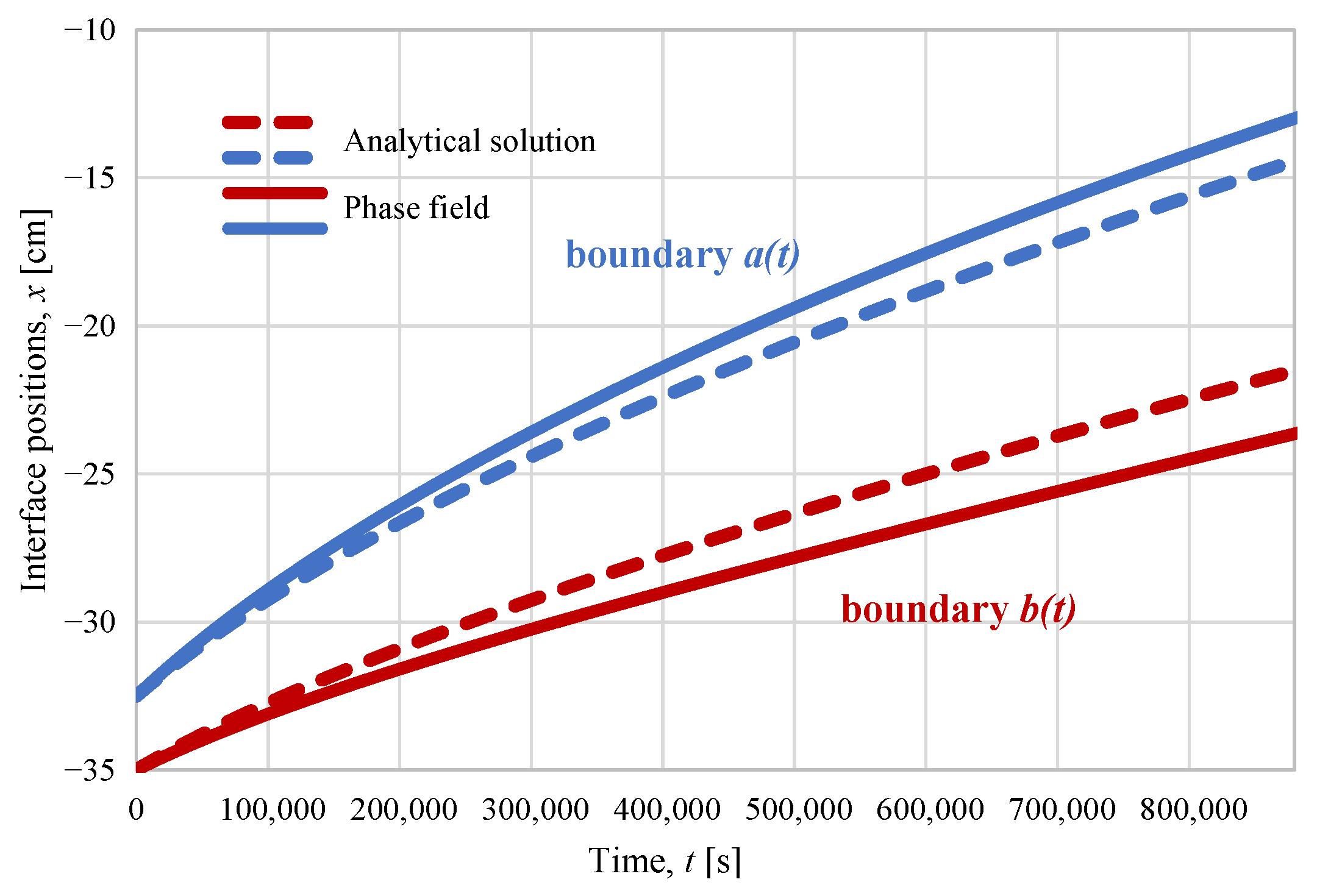
The comparison of the position of false-bottom moving boundaries for 10.25 days for the analytical model and PF simulations is provided in Figure 2. PF simulations were analyzed to extract the positions of interphase boundary, which is assumed to be at ϕ = 0.5 [46]. The fluctuations of the boundary conditions of heat flux (from the measurements of the friction velocity u [1,15,47]) smoothed and led to the expected upward migration of the false bottoms with relation to ablation under the ice floe demonstrated earlier by AIDJEX. One can find the slow thickening of the false bottom in Figure 2 which is prescribed with both analytical Equations (13) and (14) and PF Equation (21) models. The difference between the obtained data may be explained by the more accurate accounting of the heat released at the front in the PF model, which is also supported by the introduced full Gibbs energies. The rough linear liquidus line approximation of the analytical model has little effect on the resulted front position because the system exists in a narrow range of salinities, where the liquidus line is fairly straight (which is also reproduced in the PF). During periods of the thickening of false bottoms, there is a significant heat flux into the mushy layer [19] which is predicted by the analytical model for AIDJEX [19] with average value 12.9 W / m 2 . Such a flux forms a large driving force, which is naturally taken into account in PF model. However, the accuracy of the PF boundary position in the present formulation is limited by the smoothing coefficient σ C p Equation (22) and the width of the interphase boundary δ = 6 γ / W [39,48] which is controlled by the interphase barrier W and surface energy of liquid–solid interface γ . A mean difference in the positions between the models is 1.108 cm, i.e., approximately ≈6.5%, the maximum difference for a ( t ) is 1.43 cm, and 2.14 cm for b ( t ) ; the correlation coefficient is 0.999.
As a certain limitation point, it should be mentioned that both the analytical approach and the PF simulations considered here are one-dimensional (vertical) and therefore describe a horizontally averaged evolution of the false-bottom–mushy layer. Note that the lateral variability of the meltwater-lens thickness, as well as under-ice roughness, and spatial heterogeneity of near interface mixing, including double-diffusive effects, are not explicitly resolved: their net effect enters only through the prescribed forcing and bulk transfer coefficients (e.g., α h , α s ). The comparison presented in the current research should therefore be interpreted as a benchmark of the coupled thermodynamics and phase-change description and numerical implementation under prescribed boundary exchange, rather than as a full description of lateral variability in natural settings. In addition, the external forcing that controls the boundary exchange is highly variable in nature: atmospheric conditions (surface temperature and surface energy balance, which determine the conductive heat flux/temperature gradient in the ice above), as well as ocean-side conditions (e.g., T , S , and the under-ice friction velocity u ( t ) ) can change substantially on synoptic and tidal time scales. In the present work, these effects are represented by the prescribed representative values, which is sufficient for our main objective to develop the model comparison under similar boundary conditions rather than a case-specific reconstruction of all short-term environmental variability.
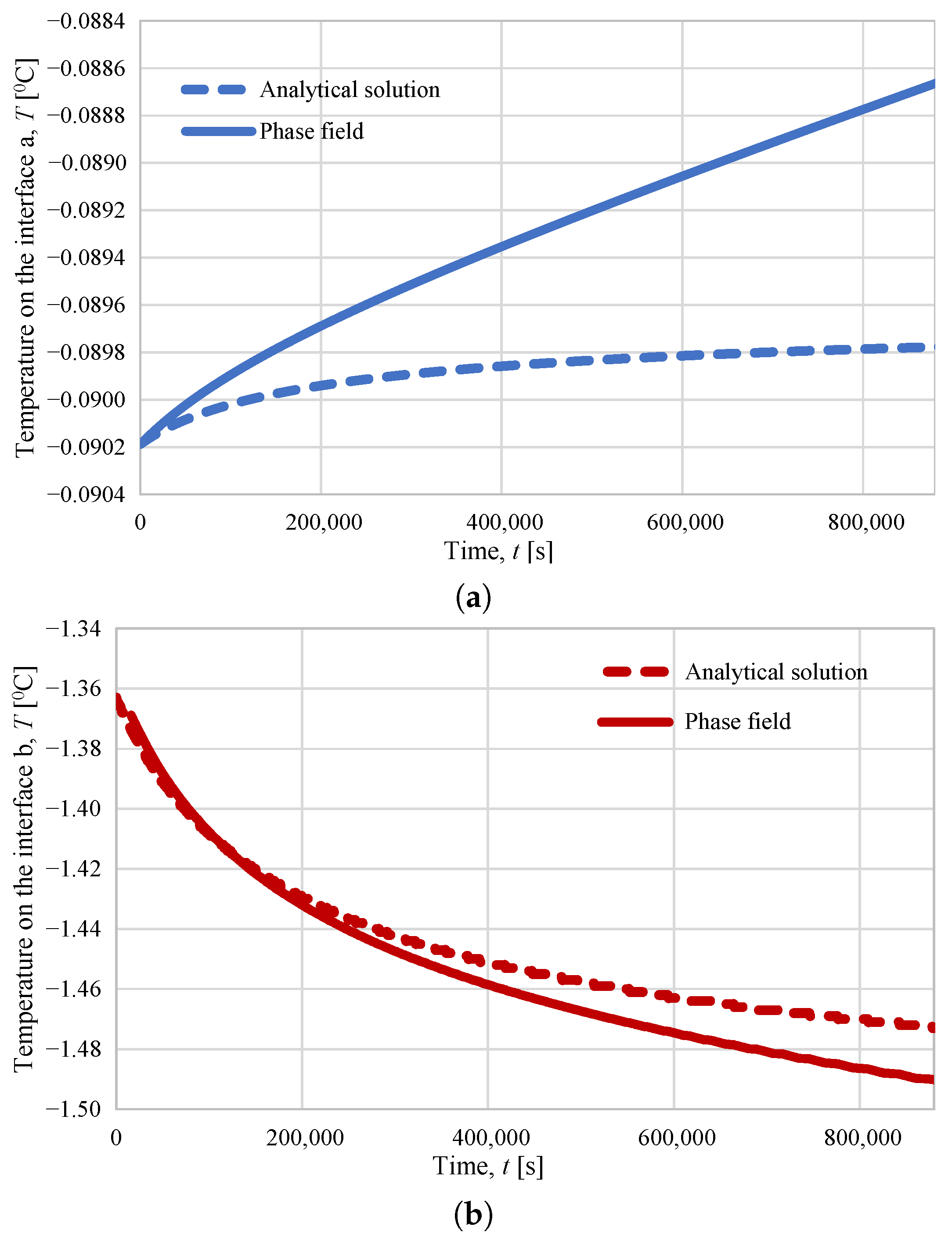
Obtained temperature variations for each moving boundary for top and bottom interfaces of the false bottom are provided in Figure 3. Although the far field temperature T can vary in natural conditions, the local false bottom boundaries temperatures control the dynamics of the ice formations. Obtained earlier, the physical properties of the mushy zone [2] as heat flux, solid fractions with a similar analytical model as provided in the present work were confirmed and allowed for quantitative agreement with the available observational data of false-bottom formation dynamics. Here, we rely on the fact that the developed analytical nonlinear model [2,35] of false-bottom dynamics accurately accounts for the physics of the process and allows for consistent quantitative estimates of the processes. Thus, we compare specific solutions with a more general PF model, taking into account the Gibbs energies of individual phases.
The temperature change shown in Figure 3a for the upper bottom boundary is shown for the phase field model and the analytical solution. The observed discrepancies are small in absolute values and comparable to the error in estimating the boundary position in the PF method. However, the observed difference in the curve shape is functional in nature. The difference in the provided solutions is caused by (i) the core assumption of the PF model which is the finite value of D c S in the solid phase and (ii) boundary conditions of the analytical model assumes that the flow of the dissolved component into fresh water above a ( t ) does not occur and the lower boundary has a fixed fraction of the solid phase ϕ b = 0.99 (almost solid). Together with the slow overall rise of the false bottom and its broadening, the fixed condition on ϕ b leads to an underestimation of the mobility of the upper boundary a ( t ) . In case of the PF model, the position of the upper boundary is controlled by the boundary conditions for the dissolved component (fresh water c = 0 at x ). Temperature T a at the crystallization front in the PF model does not reach a steady state because the flux of the solute component through the solid phase and phase boundary a ( t ) , so the upper zone of the solid phase of the false bottom continue to dilute.
In other words, for the upper interface Figure 3a, both approaches predict very close values of T a ( t ) on the considered time interval, with only a small deviation. Thus, at t 10 days the values differ by mean 5.592 × 10 4 °C (e.g., T a 0.0886 °C vs. 0.0898 °C), which corresponds to a relative difference of ≈0.6% when normalized by the PF value, with maximum difference 1.119 × 10 3 °C and correlation coefficient 0.952. The remaining difference in curvature is explained by model assumptions: in the analytical formulation, the solid fraction at the lower boundary is prescribed (Table 1), and solute transport into the fresh layer above a ( t ) is neglected, whereas in the PF simulations, a small but nonzero solute diffusivity in the solid/mushy phase allows gradual dilution and a slow shift of the local liquidus temperature; as a result, T a ( t ) in the PF model does not become perfectly stationary over the same interval.
In case of the boundary b ( t ) , see Figure 3b, solute transport is accounted for in both models, and the discrepancies are small. A mean difference is 9.084 × 10 3 °C (e.g., T b 1.47 °C vs. 1.49 °C), i.e., approximately ≈0.6%, the maximum difference is 1.838 × 10 2 °C and correlation coefficient is 0.998. The differences are most likely due to the specific way PF model accounts for the phase transition, Equation (22), with its jump in heat capacity [49]. We assume that heat transfer occurs significantly faster than the transfer of the dissolved component and the front movement, so the phase field ϕ and T equations are decoupled, simplifying the numerical simulations. However, we see differences from the simultaneously solved analytical equation in integral form, where the front’s response to concentration redistribution is relatively instantaneous. In the PF model, the T m shift along the liquidus line occurs solely due to concentration redistribution. It is important to note that, as noted above, the rate of concentration redistribution in the solid or mushy phase in the PF model is not zero [50]. In future work, we propose to validate our phase-field model against the kinetics of brine ice solidification using existing semi-analytical models, such as that of Zhen et al. [51], which has been precisely verified against cold-plate freezing experiments.
When discussing sensitivity to the turbulent heat-transfer coefficient α h , one should note that since the ocean-side heat flux in Equation (13) enters linearly through α h ρ w c w u ( T T b ) , uncertainty in α h primarily affects the predicted lower-interface evolution b ( t ) , with a monotonic response: increasing α h increases the oceanic heat supply and enhances melting at b ( t ) , while decreasing α h reduces it. The qualitative behavior of b ( t ) is robust under plausible variations of α h , while the main impact of α h is a controlled shift of the melting rate.

5. Conclusions

The formation of underwater ice layers, or “false bottoms”, exemplifies a complex, nonlinear solidification process where small-scale phase transitions significantly impact large-scale ice–ocean exchanges. The presented study bridges the gap between analytical theory and numerical phase field (PF) simulation, providing a cross-validated understanding of their dynamics.
Our comparative analysis demonstrates that the quasi-equilibrium mushy-layer model yields highly accurate, closed-form solutions for the growth rate of false bottoms under diffusion-dominated conditions, aligning well with field observations. Simultaneously, the advanced phase-field model, incorporating temperature-dependent mobility and full thermodynamic potentials, successfully captures the interface dynamics and heat redistribution controlled by solute flux. We find the general agreement between the analytical nonlinear model solved in integral form and phase field model in heat redistribution and phase boundaries’ dynamics. The PF model reveals the gradual brine drainage and non-steady thermal profiles, which emerge as the system evolves beyond the initial quasi-stationary regime.

Author Contributions

Conceptualization, I.N. and V.A.; methodology, I.N. and V.A.; software, I.N. and V.A.; validation, I.N. and V.A.; formal analysis, I.N. and V.A.; investigation, I.N. and V.A.; resources, I.N. and V.A.; data curation, I.N. and V.A.; writing—original draft preparation, I.N. and V.A.; writing—review and editing, I.N. and V.A.; visualization, I.N. and V.A.; supervision, I.N. and V.A.; project administration, I.N. and V.A.; funding acquisition, I.N. and V.A. All authors have read and agreed to the published version of the manuscript.

Funding

V. A. acknowledges financial support from the Russian Science Foundation, Russia (project no. 25-79-30012) https://rscf.ru/project/25-79-30012/ (accessed on 16 March 2026).

Data Availability Statement

The original contributions presented in this study are included in the article. Further inquiries can be directed to the corresponding author.

Conflicts of Interest

The authors declare no conflicts of interest.

Abbreviations

The following abbreviations are used in this manuscript:
PFPhase field
AIDJEXArctic Ice Dynamics Joint Experiment
SHEBASurface Heat Budget of the Arctic Ocean expedition
PDEPartial Differential Equation

References

  1. Martin, S.; Kauffman, P. The evolution of under-ice melt ponds, or double diffusion at the freezing point. J. Fluid Mech. 1974, 64, 507–528. [Google Scholar] [CrossRef] [Scilit]
  2. Alexandrov, D.V.; Nizovtseva, I.G. To the theory of underwater ice evolution, or nonlinear dynamics of “false bottoms”. Int. J. Heat Mass Transf. 2008, 51, 5204–5208. [Google Scholar] [CrossRef] [Scilit]
  3. Stefan, J. Über einige Probleme der Theorie der Wärmeleitung. Sitzungber. Wien Akad. Mat. Natur. 1889, 98, 473–484. [Google Scholar]
  4. Peixoto, J.P.; Oort, A.H. Physics of Climate; American Institute of Physics: New York, NY, USA, 1992. [Google Scholar]
  5. Scheil, E. Bemerkungen zur Schichtkristallbildung. Int. J. Mater. Res. 1942, 34, 70–72. [Google Scholar] [CrossRef] [Scilit]
  6. Flemings, M.C. Solidification Processing; McGraw-Hill Book Company: New York, NY, USA, 1974. [Google Scholar]
  7. Batchelor, G.K. Transport properties of two-phase materials with random structure. Annu. Rev. Fluid Mech. 1974, 6, 227–255. [Google Scholar] [CrossRef] [Scilit]
  8. Hills, R.; Loper, D.; Roberts, P. A thermodynamically consistent model of a mushy zone. Q. J. Mech. Appl. Math. 1983, 36, 505–539. [Google Scholar] [CrossRef] [Scilit]
  9. Fowler, A. The Formation of Freckles in Binary Alloys. IMA J. Appl. Math. 1985, 35, 159–174. [Google Scholar] [CrossRef] [Scilit]
  10. Huppert, H.; Worster, M. Dynamic solidification of a binary melt. Nature 1985, 314, 703–707. [Google Scholar] [CrossRef] [Scilit]
  11. Worster, M.G. Solidification of an alloy from a cooled boundary. J. Fluid Mech. 1986, 167, 481–501. [Google Scholar] [CrossRef] [Scilit]
  12. Worster, M.G. Convection in mushy layers. Annu. Rev. Fluid Mech. 1997, 29, 91–122. [Google Scholar] [CrossRef] [Scilit]
  13. Feltham, D.L.; Untersteiner, N.; Wettlaufer, J.S.; Worster, M.G. Sea ice is a mushy layer. Geophys. Res. Lett. 2006, 33, L14501. [Google Scholar] [CrossRef] [Scilit]
  14. Untersteiner, N.; Badgley, F. Preliminary results of thermal budget studies on Arctic pack ice during summer and autumn. Arctic Sea Ice 1958, 598, 88–92. [Google Scholar]
  15. Hanson, A.N. Studies of the mass budget of Arctic pack-ice floes. J. Glaciol. 1965, 5, 701–709. [Google Scholar] [CrossRef] [Scilit]
  16. Lyons, J.B.; Savin, S.M.; Tamburi, A.J. Basement ice, Ward Hunt Ice Shelf, Ellesmere Island, Canada. J. Glaciol. 1971, 10, 93–100. [Google Scholar] [CrossRef] [Scilit]
  17. Eicken, H. Structure of under-ice melt ponds in the central Arctic and their effect on, the sea-ice cover. Limnol. Oceanogr. 1994, 39, 682–693. [Google Scholar] [CrossRef] [Scilit]
  18. Eicken, H.; Krouse, H.R.; Kadko, D.; Perovich, D.K. Tracer studies of pathways and rates of meltwater transport through Arctic summer sea ice. J. Geophys. Res. Ocean. 2002, 107, 8046. [Google Scholar] [CrossRef] [Scilit]
  19. Notz, D.; McPhee, M.G.; Worster, M.G.; Maykut, G.; Schlünzen, A.; Heinke, K.; Eicken, H. Impact of underwater-ice evolution on Arctic summer sea ice. J. Geophys. Res. Ocean. 2003, 108, 3223–3228. [Google Scholar] [CrossRef] [Scilit]
  20. Coon, M.; Kwok, R.; Levy, G.; Pruis, M.; Schreyer, H.; Sulsky, D. Arctic Ice Dynamics Joint Experiment (AIDJEX) assumptions revisited and found inadequate. J. Geophys. Res. 2007, 112, C11S90. [Google Scholar] [CrossRef] [Scilit]
  21. Polashenski, C.; Perovich, D.; Richter-Menge, J.; Elder, B. Seasonal ice mass-balance buoys: Adapting tools to the changing Arctic. Ann. Glaciol. 2011, 52, 18–26. [Google Scholar] [CrossRef] [Scilit]
  22. Nicolaus, M.; Perovich, D.K.; Spreen, G.; Granskog, M.A.; von Albedyll, L.; Angelopoulos, M.; Anhaus, P.; Arndt, S.; Belter, H.J.; Bessonov, V.; et al. Overview of the MOSAiC expedition: Snow and sea ice. Elem. Sci. Anthr. 2022, 10, 000046. [Google Scholar] [CrossRef] [Scilit]
  23. Smith, M.M.; von Albedyll, L.; Raphael, I.A.; Lange, B.A.; Matero, I.; Salganik, E.; Webster, M.A.; Granskog, M.A.; Fong, A.; Lei, R.; et al. Quantifying false bottoms and under-ice meltwater layers beneath Arctic summer sea ice with fine-scale observations. Elem. Sci. Anthr. 2022, 10, 000116. [Google Scholar] [CrossRef] [Scilit]
  24. Salganik, E.; Katlein, C.; Lange, B.A.; Matero, I.; Lei, R.; Fong, A.A.; Fons, S.W.; Divine, D.; Oggier, M.; Castellani, G.; et al. Temporal evolution of under-ice meltwater layers and false bottoms and their impact on summer Arctic sea ice mass balance. Elem. Sci. Anthr. 2023, 11, 00035. [Google Scholar] [CrossRef] [Scilit]
  25. Alexandrov, D. Solidification with a quasiequilibrium mushy region: Exact analytical solution of nonlinear model. J. Cryst. Growth 2001, 222, 816–821. [Google Scholar] [CrossRef] [Scilit]
  26. Alexandrov, D.V.; Aseev, D.L.; Nizovtseva, I.G.; Huang, H.N.; Lee, D. Nonlinear dynamics of directional solidification with a mushy layer. Analytic solutions of the problem. Int. J. Heat Mass Transf. 2007, 50, 3616–3623. [Google Scholar] [CrossRef] [Scilit]
  27. Alexandrov, D.V.; Malygin, A.P.; Alexandrova, I.V. Solidification of leads: Approximate solutions of non-linear problem. Ann. Glaciol. 2006, 44, 118–122. [Google Scholar] [CrossRef] [Scilit]
  28. Karma, A.; Rappel, W.J. Quantitative phase-field modeling of dendritic growth in two and three dimensions. Phys. Rev. E 1998, 57, 4323–4349. [Google Scholar] [CrossRef] [Scilit]
  29. Boettinger, W.J.; Warren, J.A.; Beckermann, C.; Karma, A. Phase-field simulation of solidification. Annu. Rev. Mater. Res. 2002, 32, 163–194. [Google Scholar] [CrossRef] [Scilit]
  30. Warren, J.A.; Boettinger, W.J. Prediction of dendritic growth and microsegregation patterns in a binary alloy using the phase-field method. Acta Metall. Mater. 1995, 43, 689–703. [Google Scholar] [CrossRef] [Scilit]
  31. Provatas, N.; Elder, K. Phase-Field Methods in Materials Science and Engineering; Wiley-VCH Verlag GmbH & Co. KGaA: Weinheim, Germany, 2010; p. 312. [Google Scholar] [CrossRef] [Scilit]
  32. Echebarria, B.; Folch, R.; Karma, A.; Plapp, M. Quantitative phase-field model of alloy solidification. Phys. Rev. E 2004, 70, 061604. [Google Scholar] [CrossRef] [Scilit]
  33. Borisov, V.T. Theory of Metal-Ingot Two-Phase Zone; Metallurgiya: Moscow, Russia, 1987. [Google Scholar]
  34. Borisov, V.T. Crystallization of a Binary Alloy with Retention of Stability. Sov. Phys. Dokl. 1961, 6, 74–76. [Google Scholar]
  35. Alexandrov, D.V.; Nizovtseva, I.G. Nonlinear dynamics of the false bottom during seawater freezing. Dokl. Earth Sci. 2008, 419, 359–362. [Google Scholar] [CrossRef] [Scilit]
  36. McPhee, M.G. Turbulent stress at the ice/ocean interface and bottom surface hydraulic roughness during the SHEBA drift. J. Geophys. Res. Ocean. 2002, 107, SHE 11-1–SHE 11-15. [Google Scholar] [CrossRef] [Scilit]
  37. Kim, S.; Kim, W.T.; Suzuki, T. Phase-field model for binary alloys. Phys. Rev. E—Stat. Phys. Plasmas Fluids Relat. Interdiscip. Top. 1999, 60, 7186–7197. [Google Scholar] [CrossRef] [Scilit] [PubMed]
  38. Wang, S.L.; Sekerka, R.F.; Wheeler, A.A.; Murray, B.T.; Coriell, S.R.; Braun, R.J.; McFadden, G.B. Thermodynamically-consistent phase-field models for solidification. Phys. D Nonlinear Phenom. 1993, 69, 189–200. [Google Scholar] [CrossRef] [Scilit]
  39. Galenko, P.K.; Ankudinov, V.; Reuther, K.; Rettenmayr, M.; Salhoumi, A.; Kharanzhevskiy, E. Thermodynamics of rapid solidification and crystal growth kinetics in glass-forming alloys. Philos. Trans. R. Soc. A Math. Phys. Eng. Sci. 2019, 377, 20180205. [Google Scholar] [CrossRef] [Scilit]
  40. Nizovtseva, I.; Ankudinov, V.; Rahner, E.; Lippmann, S. Climate related phase transitions with moving boundaries by virtue of mushy zone investigation in Al–Cu: Experiment and phase-field modeling. Math. Methods Appl. Sci. 2024, 47, 6853–6867. [Google Scholar] [CrossRef] [Scilit]
  41. Gordeev, G.A.; Ankudinov, V.; Kharanzhevskiy, E.V.; Krivilyov, M.D. Numerical simulation of selective laser melting with local powder shrinkage using FEM with the refined mesh. Eur. Phys. J. Spec. Top. 2020, 229, 205–216. [Google Scholar] [CrossRef] [Scilit]
  42. Li, D.; Zeng, D.; Yin, X.; Han, H.; Guo, L.; Yao, Y. Phase diagrams and thermochemical modeling of salt lake brine systems. II. NaCl + H2O, KCl + H2O, MgCl2 + H2O and CaCl2 + H2O systems. Calphad Comput. Coupling Phase Diagrams Thermochem. 2016, 53, 78–89. [Google Scholar] [CrossRef] [Scilit]
  43. Fang, Y.; Liu, D.; Zhu, Y.; Galenko, P.; Lippmann, S. Observation of Pattern Formation during Electromagnetic Levitation Using High-Speed Thermography. Crystals 2022, 12, 1691. [Google Scholar] [CrossRef] [Scilit]
  44. Soundararajan, B.; Sofia, D.; Barletta, D.; Poletto, M. Review on modeling techniques for powder bed fusion processes based on physical principles. Addit. Manuf. 2021, 47, 102336. [Google Scholar] [CrossRef] [Scilit]
  45. COMSOL AB. COMSOL Multiphysics® v. 6.0; COMSOL AB: Stockholm, Sweden, 2022. [Google Scholar]
  46. Moelans, N.; Blanpain, B.; Wollants, P. An introduction to phase-field modeling of microstructure evolution. Calphad 2008, 32, 268–294. [Google Scholar] [CrossRef] [Scilit]
  47. McPhee, M.G. Turbulent heat flux in the upper ocean under sea ice. J. Geophys. Res. 1992, 97, 5365–5379. [Google Scholar] [CrossRef] [Scilit]
  48. Karma, A. Phase-Field Formulation for Quantitative Modeling of Alloy Solidification. Phys. Rev. Lett. 2001, 87, 115701. [Google Scholar] [CrossRef] [Scilit]
  49. Voller, V.; Cross, M. Accurate solutions of moving boundary problems using the enthalpy method. Int. J. Heat Mass Transf. 1981, 24, 545–556. [Google Scholar] [CrossRef] [Scilit]
  50. Notz, D.; Worster, M.G. Desalination processes of sea ice revisited. J. Geophys. Res. Ocean. 2009, 114, C05006. [Google Scholar] [CrossRef] [Scilit]
  51. Zhen, Z.; Song, M.; Cai, B.; Zhang, X.; Liu, Z.; Gao, R. Experimental and modeling studies on the growth characteristics of ice layers at different temperatures and salinities. Int. J. Heat Fluid Flow 2025, 115, 109868. [Google Scholar] [CrossRef] [Scilit]
Figure 1. A sketch of an under-ice fresh water pond [1,2] and a schematic diagram of the process with designated moving interface boundaries a ( t ) and b ( t ) .
Mathematics 14 01040 g001
Figure 2. Dynamics of the interface boundaries a ( t ) and b ( t ) (see Figure 1), given for the analytical integral solution of Equations (13) and (14) and the numerical solution of Equation (21).
Mathematics 14 01040 g002
Figure 3. Comparison of the temperatures T on interface boundaries: (a) T a on a ( t ) and (b) T b on b ( t ) , given for analytical integral solution of Equations (13) and (14) and numerical solution of Equation (21).
Mathematics 14 01040 g003
Table 1. Properties and model parameters used for the NaCl–H2O false-bottom problem analytical solution and phase-field simulations.
PropertyValueSourcePropertyValueSource
φ b (init) (-) 0.99 [2]u (cm/s)tabular data[2,19,36]
T (°C) 1.5 [2]m (°C/wt%)53[2]
L v (J/( cm 3 )) 308.16 [2] a ( 0 ) b ( 0 ) (cm) 2.5 [2]
k w (J/(cm c °C)) 5.86 × 10 3 [2] k i (J/(cm c °C)) 22.19 × 10 3 [2]
α h (-) 0.0095 [2] α h / α s (-)35[2]
S (psu)29.8[2] c (fraction wt%)2.98[2]
T e (K)252[42] c e (fraction wt%)24[42]
a 1 (-)36.191current work a 3 (-)4.125current work
a 2 (-)9054.897current work a 4 (-)−1031.373current work
Disclaimer/Publisher’s Note: The statements, opinions and data contained in all publications are solely those of the individual author(s) and contributor(s) and not of MDPI and/or the editor(s). MDPI and/or the editor(s) disclaim responsibility for any injury to people or property resulting from any ideas, methods, instructions or products referred to in the content.