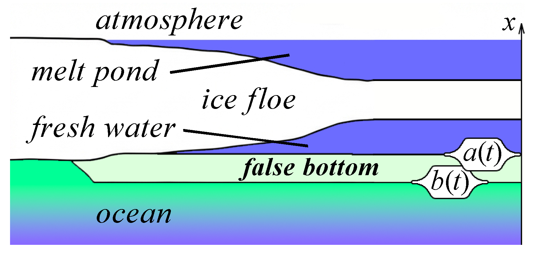
2. The Nonlinear Analytical Model of “False Bottom” Evolution
In order to describe the nonlinear solidification dynamics of a false bottom, we employ a one-dimensional analytical model of the growing ice layer as a mushy zone of ice (solid phase) and sea water (liquid phase). This approach follows the quasi-equilibrium mushy-layer theory developed in prior works, e.g., Borisov’s model [
33,
34] and its extensions, solved analytically by Alexandrov et al. [
25] for binary alloy solidification. There the exact solution was obtained for a unidirectional freezing problem with a mushy region, yielding explicit profiles for temperature, concentration, and solid fraction, as well as an algebraic relation for the solid fraction at the mush–solid interface.
Based on these points, we formulate the false-bottom problem with similar assumptions (as in [
2,
25]): (i) a quasi-steady temperature profile across the mushy zone; (ii) immediate local phase equilibration; and (iii) one-dimensional diffusive transport of heat and solute. A set of governing Equations (
1)–(
7) is provided below considering the conservation of energy and salt in the mushy layer and at its moving boundaries, followed by analytical solutions (
8)–(
14) that describe the evolution.
We specify the temperature and salinity fields inside the false bottom: under the quasi-equilibrium assumption, heat diffuses rapidly compared to the timescale of interface motion, so the temperature in the mushy layer can be approximated as linear in space at any given time. Accordingly, Equation (
1) governs the evolution of salinity within the mushy zone (false bottom) by accounting for both diffusive transport and the effects of phase change:
Here
is the volume fraction of solid (ice) at position
and time
within the mush, so
is the liquid fraction (brine porosity). Likewise
is the salinity of the liquid in the pores (often taken nondimensionally, e.g., relative to the far-field salinity
). The left-hand side of Equation (
1) represents the local rate of change of salt in the liquid portion of the mush. This changes due to two processes: (i) the diffusion of salt along the mushy layer, the first term on the right, and (ii) the redistribution of salt when liquid solidifies, the second term on the right). Physically, Equation (
1) encapsulates constitutional freezing: as ice forms in the mush, salt is rejected or absorbed according to the partition ratio, and the excess salt diffuses away into the surrounding brine. This ensures salinity is redistributed within the mushy layer in step with ice crystallization. Equation (
2) governs the temperature field
in the mushy zone, assuming thermal diffusion is fast enough that the process is quasi-steady in time (no explicit
term):
Equation (
3) imposes the phase equilibrium condition that couples the temperature and salinity in the two-phase region:
where
is a reference freezing temperature (e.g., the melting point of pure water in the chosen units) and
m is the liquidus slope (the rate at which the freezing point decreases with increasing salinity). This linear relation
(in dimensional terms) corresponds to the liquidus equation from the phase diagram
.
Equation (
3) implies quasi-equilibrium assumption: the mushy zone is always at the phase boundary, with solid and liquid in thermodynamic equilibrium. Physically, this means that latent heat release has eliminated any thermal undercooling in the pores—the brine is as cold as it can be without freezing further. The temperature variable is eliminated from the mush equations: substituting the linear Equation (
3) into Equation (
2) effectively couples the heat and mass conservation laws into a single description.
The external thermal and solutal environment is defined with the Equation (
4) in the far-field limit Equation (
5):
Far enough from the mushy zone the ocean salinity tends to
, the ambient sea salinity, and the temperatures vary linearly with depth at fixed gradients
and
. These serve as boundary conditions for solving the mushy-zone equations. We note that in Equation (
4) diffusion in the solid ice is neglected which is a valid approximation since molecular salt diffusion in solid ice is practically zero, and the ice above is treated as a boundary with a fixed gradient rather than a time-evolving field, while in the phase-field model, diffusion in the solid phase is taken to be very small, but non-zero, in order to maintain continuity and numerical stability:
Equations (
6) and (
7) are written in the standard nondimensional quasi-equilibrium mushy-layer notation and are shown here to represent the structure of the energy and salt balances at the moving boundary
. In the false-bottom setting, we apply analogous Stefan-type balances at each moving interface and rewrite them in dimensional variables using
and
and the mixture conductivity
(see also Equations (
11)–(
14) below). The notational difference
versus
reflects the quasi-stationary traveling-wave reduction (nearly constant interface speed over the considered interval) versus the time-dependent interface tracking used in the comparison. Finally, the latent-heat term is weighted by the phase fraction that actually undergoes phase change at the considered boundary (freezing of liquid into a mushy mixture vs. the solidification/melting of the residual liquid–solid within a mush). We also assume the convention is evaluated on the mushy side with the normal pointing from the mush, so the sign of the gradient is consistent throughout.
Under the above governing equations, one can obtain an exact analytical solution [
2,
35] for the steady growth of the false bottom in a diffusion-dominated regime. The solution assumes a quasi-stationary solidification: the mushy layer profiles attain a self-similar form moving with the interface velocities. In particular, the upper interface
advances with a nearly constant speed
, and the mushy zone reaches a steady thickness
(or a slowly varying thickness that can be treated as approximately constant during early growth). These assumptions convert the partial differential system into an ODE boundary-value problem, which can be solved in closed form. Note that in the present paper we use these closed-form relations as the analytical reference for the comparison with the further PF simulations: a step-by-step reduction from the governing mushy-layer system to the integral relations is available in the primary derivations of the false-bottom theory and the underlying quasi-equilibrium mushy-layer solution as developed in [
2,
25].
The result is given by Equations (
8)–(
14) which describe the internal profiles of temperature, salinity, and solid fraction in the mush. We also keep in mind that while in (1)–(7) we follow the notation commonly used in the original quasi-equilibrium mushy-layer formulation, where, for example,
denotes temperature and
denotes salinity, starting from Equation (
8) and throughout, we use the dimensional variables
T and
S for temperature and salinity, while the solute field in the PF model is denoted by the mass fraction
c. Thus, the exact solution shows that the temperature in the mushy zone varies linearly with position between the two boundaries:
Physically, a linear
T-profile means there are no internal heat sources or sinks in the mush besides the phase change at the boundaries. In this case all latent heat release is balanced by conduction, resulting in a uniform gradient. By the equilibrium condition,
and
correspond to the liquidus temperatures of the interface salinities
and
respectively (see (
10) below). Equation (
8) thus provides an exact temperature profile across the false bottom, showing a smooth linear drop from the warmer upper interface
to the colder lower interface
, assuming
in typical scenarios.
Within the quasi-stationary self-similar reduction used to obtain the integral relations, the salinity solution yields an invariant: the product
becomes stationary in the reduced (moving-frame) description of the mushy layer [
25], namely
Equation (
9) should therefore be understood as a property of the quasi-stationary integral solution, steady in the moving frame, rather than as a general identity of the full time-dependent PDE system without these assumptions.
Physically, as the false bottom grows or evolves, the internal distribution of brine and solid adjusts such that the product of liquid fraction and salinity stays constant. If, for example, the solid fraction
increases at some location, the liquid salinity
there must drop proportionally to keep
fixed (the brine is being diluted exactly as pores fill with ice). This behavior is characteristic of self-similar solidification solutions. In practice, one can determine
as a function of
x from the initial conditions or from integrating the steady-state form of Equation (
1), and that profile then applies for all subsequent times until the assumptions break down.
Equation (
10) restates the local equilibrium condition (
3) in the dimensional variables of the solution,
We see that within the mushy layer, at any position
x and time
t, the temperature
is exactly the freezing point corresponding to the local salinity
. In this form,
from Equation (
3) has been set to 0 by choosing the reference temperature as the melting point of pure ice so that
; one can always shift
T by a constant without loss of generality. This equation emphasizes that the mush operates on the liquidus curve.
Equation (
10) is used in practice to relate the interface temperatures and salinities, while the following (
11) gives the rate of advance of the upper mush–ice interface, incorporating the effect of partial solid fraction at that boundary:
The left side of Equation (
11) represents the latent heat released per unit area per unit time as the interface moves, while the right-hand side represents the heat flux conducted away from the interface. Equation (
11) therefore states that the latent heat released by freezing at the upper interface is carried off by thermal conduction into the surrounding material. It is a rearranged Stefan condition tailored to a mushy interface, compare to Equation (
6) earlier. This equation yields the growth rate of the false-bottom’s top
as a function of the prevailing heat flux: the stronger the thermal gradient into the cold ice above, the faster the freshwater freezes onto the false bottom. Furthermore
is the counterpart of Equation (
7) in the final solution form (in dimensional variables). It equates the rate of salt advection by the moving interface to the diffusive salt flux at that interface.
Thus Equation (
12) demands that any salt displaced by upward freezing is immediately diffused back into the mushy layer. In the limit that the upper interface is freezing pure water (initial freshwater lens) with
, the left side is nearly zero, which means there is no jump of salinity. Accordingly, the salinity gradient at the top of the mush
adjusts to zero in that case. More generally, Equation (
12) ensures a smooth salinity profile at the interface: it prevents a salinity discontinuity at
by expelling or absorbing salt via diffusion as the false bottom accretes fresh ice on top. This condition would be used together with Equation (
11) to solve for the evolution of
and
at the interface: it links the interface motion to the salinity gradient just below the interface, and thereby to the changing salinity of the pore brine at that boundary.
Equation (
13) is the Stefan condition at the ice–ocean interface
; it balances the latent heat released by freezing with the heat fluxes at that boundary. The left-hand side here is the latent heat per unit area released as the mushy layer advances at velocity
, while the right-hand side represents the conductive heat flux out of the interface using the local mixture of ice and water with thermal conductivities
and
:
Here the last term is a standard bulk (Stanton-number type) parameterization of the turbulent ocean-side heat flux at the ice–ocean boundary:
sets the turbulent transport scale with
u taken from the under-ice friction-velocity forcing used in the false-bottom datasets, while
is a dimensionless transfer coefficient that lumps the unresolved boundary-layer physics into a single effective parameter. In this work we take
from the established parameter set used in the original false-bottom theory [
2] based on AIDJEX/SHEBA data forcing in order to keep the analytical and PF comparisons under identical boundary exchange conditions.
Generally, one uses Equation (
13) to find the rollback or advance rate of the lower interface
given: a larger
(warmer ocean) or higher
(more vigorous heat transfer) will increase the melting flux. Our analytical model’s inclusion of this convective term is a crucial adaptation for underwater ice formation—it further extends Alexandrov’s mushy-layer solution [
2,
35] by accounting for the finite heat flux from seawater.
The salt balance at the ice–ocean interface
is given by
The left-hand side is the rate of salt pulling due to interface development (with
the brine salinity at the interface and
the local solid fraction in the mushy zone). This is balanced by the convective salt flux, which carries away excess salt into the ocean, proportional to the flow velocity
u and the salinity difference between the far-field water
and the interface brine
.
To obtain the dynamics of the top
and bottom
boundary interfaces, we utilize the Alexandrov’s integral solution [
2,
35] with initial and boundary conditions defined with the experimental data on false bottom evolution taken from the AIDJEX and the SHEBA field experiments [
19,
36] (provided below in
Section 3).
3. Phase Field Diffuse Interface Model of Water Solidification
In the present study, we use a one-dimensional phase-field (PF) model for an aqueous NaCl solution, formulated in terms of a solid–liquid order parameter
(
liquid and
solid), the solute mass-fraction field
, and the temperature field
. The free-energy density Equation (
15) includes bulk and interfacial contributions and provides a temperature-dependent thermodynamic driving force for phase transformation, consistent with established PF formulations for binary systems [
31,
37] which is based on the thermodynamically consistent approach [
38,
39]. We consider the solid–liquid phase transition and latent heat release introduced with the heat capacity leap
dependent on the solute concentration and
T [
40,
41]. The region of low solute concentrations of an aqueous NaCl solution (salinity of sea water
psu, which is equal to
wt% NaCl) has been investigated, and thus we neglect the chemical interaction contribution considering linear solidus and liquidus lines as well as the absence of additional chemical interactions in the liquid phase.
One can determine a complete PF free energy functional of a binary solution as
Here one considers a certain deviation from the reference free energy
, Equation (
15), where
V is the volume of the domain,
is the gradient energy coefficient related to the solid–liquid interface energy, and
is the coefficient which defines the length scales of the compositional boundary [
31,
39]. Here the concentration
c is treated as a mass fraction (
), which corresponds to 0–100 wt% NaCl; in particular,
denotes fresh water.
We consider only the slow phase-transitions and so the contributions of the non-equilibrium terms, such as first- and second-order fluxes of the order parameter, are vastly small. We extend and modify existing PF models [
37,
38,
39,
40] to properly account for the realistic Gibbs energies in the presence of a small temperature gradient.
The equilibrium contribution of the free energy density
could be written as
where the separate contributions
and
are obtained from a thermodynamic database and are related to the free energy in Equation (
16) by the limiting cases:
for the solid, and
for the liquid phase. Here
corresponds to the fresh water, and
is the saline composition at the eutectic point (
K,
wt%):
This form includes the Gibbs energies of liquid phase
, which were implemented as a temperature-dependent Gibbs energy contributions, aqueous solutions of NaCl ions
, and the ice
(see phase diagram and Gibbs energy coefficients for the NaCl + H
2O system in [
42]).
The function
is a phenomenological interpolation function with values
and
[
38,
39]. The
function is a wall of a simple double-well potential [
31,
37,
39]:
For the eutectic diluted aqueous solution one can assume the liquid phase to be ideal, which leads to
in Equation (
16). However, the description of the non-ideal mixture in the region of the higher concentration can be improved with the Redlich–Kister expansion with relevant coefficients [
43]. A non-ideal solid is described using the empirical form of
as [
31,
37]:
where specific values of the constants
are to be determined from thermodynamic conditions in the eutectic point. Specific values of coefficients
,
,
,
might be obtained from the conditions on the free energies at the eutectic point
,
, such as
,
and a common tangent construction (values are represented in
Table 1).
A stable evolution of the entire system is given by the Lyapunov condition of a non-positive change of the total free energy Equation (
15) in time from which one can obtain a dynamical equation as a functional derivative separately for conserved
c and non-conserved
order parameters [
31,
39]:
Coupling PF with the heat transfer equation was provided with the introduction of the temperature variable
T into PF model. At the same time, a response of the thermophysical properties is retrieved from the consideration of the phase transition as a finite leap of the heat capacity
[
40,
41]:
where composition-dependent melting temperature
followed from the liquidus slope
m and current concentration; the smoothing coefficient
°C describes the width of the heat capacity leap associated with the latent heat of fusion. This implementation is based on the normalization of the finite leap on the enthalpy of fusion
. Such a leap describes the finite width of the liquidus–solidus range and allows one to introduce the mushy zone. The method with an effective heat capacity coefficient accounting
for the phase transition has proven effective for the modeling of the wide spectra of the heat transfer problems with high- and low-temperature gradients [
40,
41,
44].
The concentration diffusion between solid and liquid phases has been introduced as a phase-dependent diffusion coefficient
as a tanh-like step from
to
. In the present model we consider a temperature-dependent heat diffusivity
, heat capacity
and density
for a fixed composition of
[
42]. The latent enthalpy of fusion of the composition of phases is defined as a linear mixture of
and
.
Numerical simulations were performed with the same boundary conditions as stated for analytical model Equations (
13) and (
14) with the constants (
Table 1) and thermophysical properties obtained from thermodynamical data [
42]. The single-dimensional task was prepared with a mesh size of
mm for a domain with a length of 1 m. The presented task was solved using finite element method with the PARDISO direct solver in COMSOL Multiphysics 6.0 software [
45] with the adaptive step for time integration. The segregated solver with fixed limits on concentration
c and PF
variables were utilized. All calculations were performed on a two-processor AMD Epyc-based computer.
4. Results and Discussion
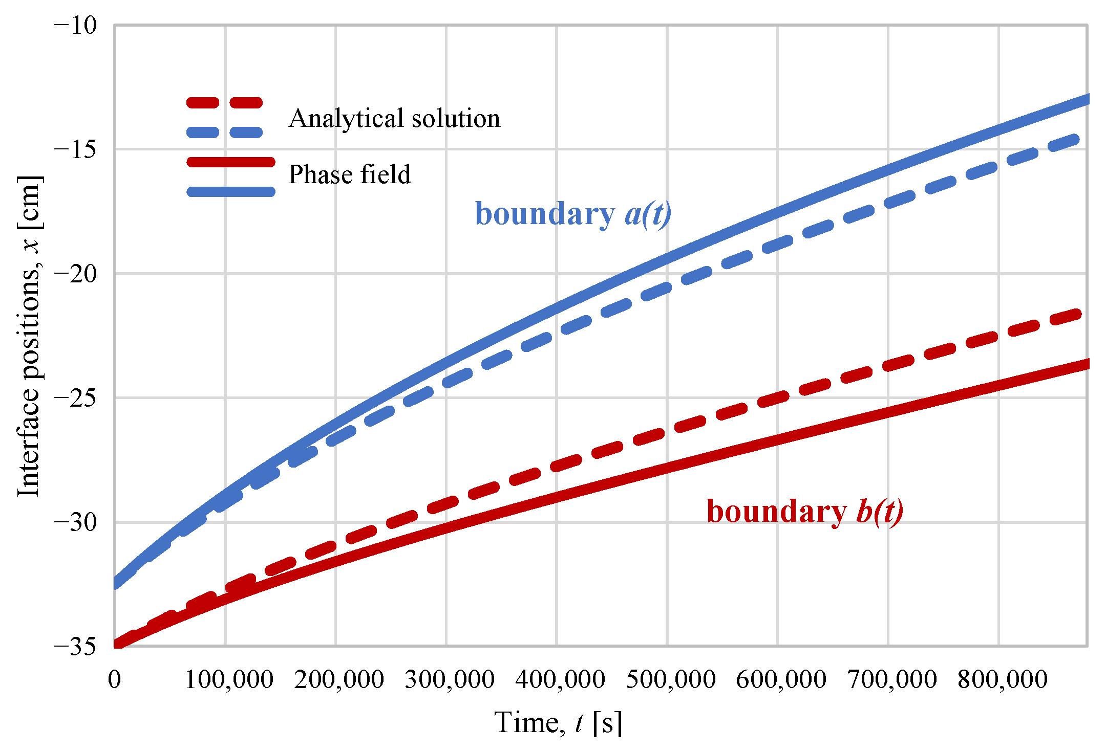
The comparison of the position of false-bottom moving boundaries for 10.25 days for the analytical model and PF simulations is provided in
Figure 2. PF simulations were analyzed to extract the positions of interphase boundary, which is assumed to be at
[
46]. The fluctuations of the boundary conditions of heat flux (from the measurements of the friction velocity
u [
1,
15,
47]) smoothed and led to the expected upward migration of the false bottoms with relation to ablation under the ice floe demonstrated earlier by AIDJEX. One can find the slow thickening of the false bottom in
Figure 2 which is prescribed with both analytical Equations (
13) and (
14) and PF Equation (
21) models. The difference between the obtained data may be explained by the more accurate accounting of the heat released at the front in the PF model, which is also supported by the introduced full Gibbs energies. The rough linear liquidus line approximation of the analytical model has little effect on the resulted front position because the system exists in a narrow range of salinities, where the liquidus line is fairly straight (which is also reproduced in the PF). During periods of the thickening of false bottoms, there is a significant heat flux into the mushy layer [
19] which is predicted by the analytical model for AIDJEX [
19] with average value 12.9
. Such a flux forms a large driving force, which is naturally taken into account in PF model. However, the accuracy of the PF boundary position in the present formulation is limited by the smoothing coefficient
Equation (
22) and the width of the interphase boundary
[
39,
48] which is controlled by the interphase barrier
W and surface energy of liquid–solid interface
. A mean difference in the positions between the models is 1.108 cm, i.e., approximately ≈6.5%, the maximum difference for
is 1.43 cm, and 2.14 cm for
; the correlation coefficient is 0.999.
As a certain limitation point, it should be mentioned that both the analytical approach and the PF simulations considered here are one-dimensional (vertical) and therefore describe a horizontally averaged evolution of the false-bottom–mushy layer. Note that the lateral variability of the meltwater-lens thickness, as well as under-ice roughness, and spatial heterogeneity of near interface mixing, including double-diffusive effects, are not explicitly resolved: their net effect enters only through the prescribed forcing and bulk transfer coefficients (e.g., , ). The comparison presented in the current research should therefore be interpreted as a benchmark of the coupled thermodynamics and phase-change description and numerical implementation under prescribed boundary exchange, rather than as a full description of lateral variability in natural settings. In addition, the external forcing that controls the boundary exchange is highly variable in nature: atmospheric conditions (surface temperature and surface energy balance, which determine the conductive heat flux/temperature gradient in the ice above), as well as ocean-side conditions (e.g., , , and the under-ice friction velocity ) can change substantially on synoptic and tidal time scales. In the present work, these effects are represented by the prescribed representative values, which is sufficient for our main objective to develop the model comparison under similar boundary conditions rather than a case-specific reconstruction of all short-term environmental variability.
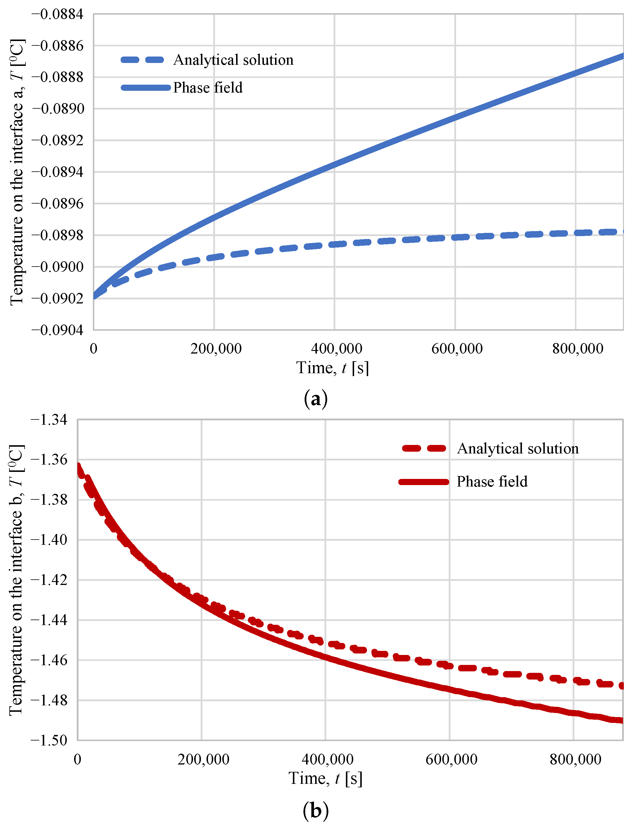
Obtained temperature variations for each moving boundary for top and bottom interfaces of the false bottom are provided in
Figure 3. Although the far field temperature
can vary in natural conditions, the local false bottom boundaries temperatures control the dynamics of the ice formations. Obtained earlier, the physical properties of the mushy zone [
2] as heat flux, solid fractions with a similar analytical model as provided in the present work were confirmed and allowed for quantitative agreement with the available observational data of false-bottom formation dynamics. Here, we rely on the fact that the developed analytical nonlinear model [
2,
35] of false-bottom dynamics accurately accounts for the physics of the process and allows for consistent quantitative estimates of the processes. Thus, we compare specific solutions with a more general PF model, taking into account the Gibbs energies of individual phases.
The temperature change shown in
Figure 3a for the upper bottom boundary is shown for the phase field model and the analytical solution. The observed discrepancies are small in absolute values and comparable to the error in estimating the boundary position in the PF method. However, the observed difference in the curve shape is functional in nature. The difference in the provided solutions is caused by (i) the core assumption of the PF model which is the finite value of
in the solid phase and (ii) boundary conditions of the analytical model assumes that the flow of the dissolved component into fresh water above
does not occur and the lower boundary has a fixed fraction of the solid phase
(almost solid). Together with the slow overall rise of the false bottom and its broadening, the fixed condition on
leads to an underestimation of the mobility of the upper boundary
. In case of the PF model, the position of the upper boundary is controlled by the boundary conditions for the dissolved component (fresh water
at
). Temperature
at the crystallization front in the PF model does not reach a steady state because the flux of the solute component through the solid phase and phase boundary
, so the upper zone of the solid phase of the false bottom continue to dilute.
In other words, for the upper interface
Figure 3a, both approaches predict very close values of
on the considered time interval, with only a small deviation. Thus, at
days the values differ by mean
°C (e.g.,
°C vs.
°C), which corresponds to a relative difference of ≈0.6% when normalized by the PF value, with maximum difference
°C and correlation coefficient 0.952. The remaining difference in curvature is explained by model assumptions: in the analytical formulation, the solid fraction at the lower boundary is prescribed (
Table 1), and solute transport into the fresh layer above
is neglected, whereas in the PF simulations, a small but nonzero solute diffusivity in the solid/mushy phase allows gradual dilution and a slow shift of the local liquidus temperature; as a result,
in the PF model does not become perfectly stationary over the same interval.
In case of the boundary
, see
Figure 3b, solute transport is accounted for in both models, and the discrepancies are small. A mean difference is
°C (e.g.,
°C vs.
°C), i.e., approximately ≈0.6%, the maximum difference is
°C and correlation coefficient is 0.998. The differences are most likely due to the specific way PF model accounts for the phase transition, Equation (
22), with its jump in heat capacity [
49]. We assume that heat transfer occurs significantly faster than the transfer of the dissolved component and the front movement, so the phase field
and
T equations are decoupled, simplifying the numerical simulations. However, we see differences from the simultaneously solved analytical equation in integral form, where the front’s response to concentration redistribution is relatively instantaneous. In the PF model, the
shift along the liquidus line occurs solely due to concentration redistribution. It is important to note that, as noted above, the rate of concentration redistribution in the solid or mushy phase in the PF model is not zero [
50]. In future work, we propose to validate our phase-field model against the kinetics of brine ice solidification using existing semi-analytical models, such as that of Zhen et al. [
51], which has been precisely verified against cold-plate freezing experiments.
When discussing sensitivity to the turbulent heat-transfer coefficient
, one should note that since the ocean-side heat flux in Equation (
13) enters linearly through
, uncertainty in
primarily affects the predicted lower-interface evolution
, with a monotonic response: increasing
increases the oceanic heat supply and enhances melting at
, while decreasing
reduces it. The qualitative behavior of
is robust under plausible variations of
, while the main impact of
is a controlled shift of the melting rate.