In this section, numerical experiments are conducted on the DFJSP using GP, PF-GP [
5], APF-GP-
[
6], and APF-GP-
to verify the effectiveness of the proposed method.
3.1. Experimental Setup
is determined by the weighted sum of the arrival time of the
-th job set and the makespan
of the schedule created by adding the
d-th job set, as shown in Equation (
7):
In the experiments, the number of job set arrivals is set to 30, and the
d-th job set is assumed to arrive at time
. This experimental setup is adopted to generate new job sets, representing dynamic changes, only after the previously scheduled processing has sufficiently progressed. This allows for the evaluation of both the performance of the generated schedules and the capability to respond to dynamic changes. The number of jobs in each set is defined as the number of jobs whose operations were all completed between the arrival of the previous job set and the arrival of the new one.
The number of machines capable of processing each operation,
, and the index of these machines,
, are determined as follows, where
and
are uniform random numbers in the range
, and
M is the total number of machines available simultaneously:
In this experiment, a scenario is considered where the characteristics of the arriving job sets vary with a cycle of 12. This is achieved by varying the maximum operation processing time
s and the variable
t, which determines the tightness of due dates, with cycles of 4 and 3, respectively, upon each job set arrival, as described below:
This approach can reproduce the scheduling of orders and production with mid-to-long-term cycles—such as seasonal patterns and market trends observed in actual production sites—as well as weekly and monthly production plans. Therefore, this paper conducts simulations using job sets possessing periodic characteristics. The processing time
of the operations of job
i in the newly arriving
d-th job set, the ready time (earliest start time)
, and the due date
are determined using uniform random numbers
as follows:
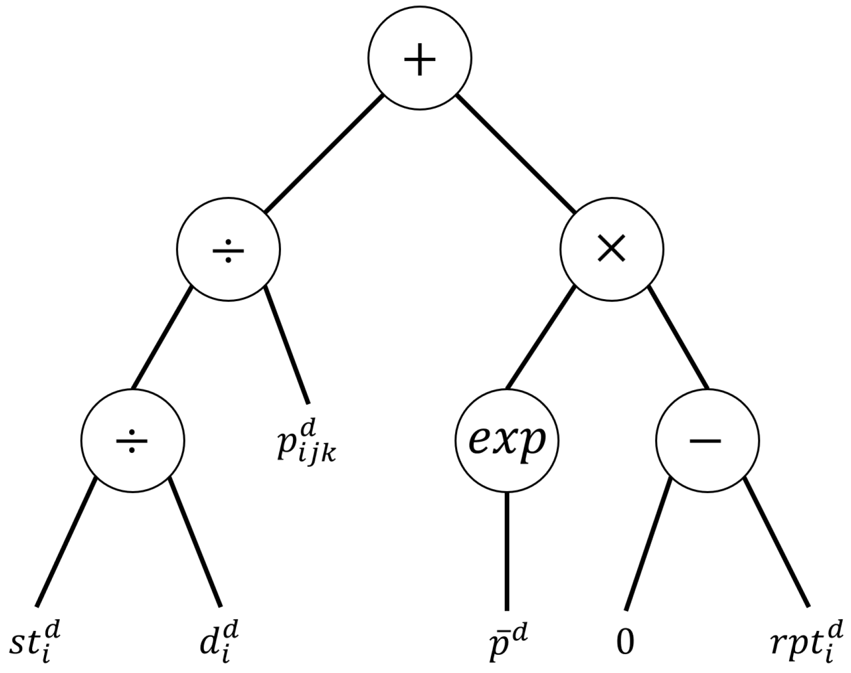
Each individual in GP uses the representation format of MTGP [
12]. For each generation, scheduling is performed using the best individual. If the objective function value
E obtained from the scheduling has not been improved for 30 consecutive generations during the search process, the solution is interpreted to have converged, and the search is terminated. The parameters used in this experiment are shown in
Table 2.
The experiments were conducted on a computer equipped with an 11th Gen Intel(R) Core(TM) i7-11700 processor, 16.0 GB RAM, and Intel(R) UHD Graphics 750. The software environment consisted of Windows 11, Python 3.10.9, and NumPy 1.25.2.
3.2. Numerical Results
To compare GP [
2], PF-GP [
5], APF-GP-
[
6], and APF-GP-
, ten trial runs were conducted for the scheduling problems with the number of jobs and operations shown in
Table 3.
Table 4,
Table 5,
Table 6 and
Table 7 show the experimental results for each method, including the average objective function value, the average makespan
, the total tardiness of all jobs
, the computation time, and the average total number of generations across ten trials. These tables also provide a comparison of the average objective function values between the proposed method and conventional GP and PF-GP. Wilcoxon rank-sum tests were performed at a significance level of 5%. In the comparison results, “+” indicates that the objective function value is significantly larger (worse) than the comparative target, “−” indicates that it is significantly smaller (better), and “≈” indicates no significant difference. Additionally,
Table 8 shows the ratio of the computation time for each scenario relative to that of PF-GP.
From
Table 4,
Table 5,
Table 6 and
Table 7, in Scenarios (10, 4), (10, 6), and (15, 6), PF-GP achieves better objective values than GP with approximately the same computation time. While APF-GP-
and APF-GP-
show worse objective values than PF-GP, they substantially reduce the computation time. Furthermore, APF-GP-
requires less computation time, whereas APF-GP-
provides better objective values.
Focusing solely on the objective values, PF-GP is significantly better than GP in Scenarios (10, 4) and (10, 6). While APF-GP-
is significantly worse than PF-GP in Scenarios (10, 6) and (15, 6), APF-GP-
is significantly worse only in Scenario (10, 6). In Scenario (10, 6), the objective function value obtained by APF-GP is inferior to that of PF-GP. This is because, in Scenario (10, 6), cases where tardiness occurs—which is heavily weighted and prioritized in Equation (
1)—are rare, and the makespan accounts for a larger proportion of the objective function value. APF-GP evaluates the increase in population size based on the degree of improvement in the objective function. Consequently, improvements in makespan, which have a smaller impact on the overall value, are given lower priority, leading the algorithm to prioritize reducing computational time in such cases. Therefore, it is considered that APF-GP prioritized computational time more than in other scenarios, resulting in objective function values significantly worse than those of PF-GP in Scenario (10, 6). Furthermore, when no tardiness occurs, the increase rate is switched to
. This explains why the differences in objective function values and computational times between APF-GP-
and APF-GP-
are smaller. These results suggest that APF-GP-
is more appropriate for scheduling in environments like Scenario (10, 6), where tardiness is unlikely to occur and the objective is to reduce computational time.
As shown in
Table 8, compared to PF-GP, APF-GP-
drastically reduces the computation time to approximately 35–
, and APF-GP-
reduces it to approximately 50–
.
3.3. Analysis of Population Increase Rates
To compare APF-GP- and APF-GP-, the relationship between the objective values and the number of evaluations for each scheduling task is analyzed. In the experiments in this section, to strictly compare the optimization results of the scheduling for each job set arrival, an experimental setup is employed where the state of the remaining jobs at the time of each job set arrival is kept identical. Specifically, to synchronize the uncompleted jobs at the time a new job set arrives, pre-processing is performed on the jobs based on a common rule obtained via PF-GP. A situation is set where a new job set arrives during this process. Subsequently, all uncompleted jobs, including the newly arrived ones, are rescheduled according to the same pre-defined rules. The repetition of this operation clarifies the performance difference between the two methods. This procedure standardizes the influence of remaining jobs across all trials at the time of a job set arrival, making it ideal for analyzing the impact of each individual arrival.
Ten trial runs were conducted for the scheduling problems given in
Table 3.
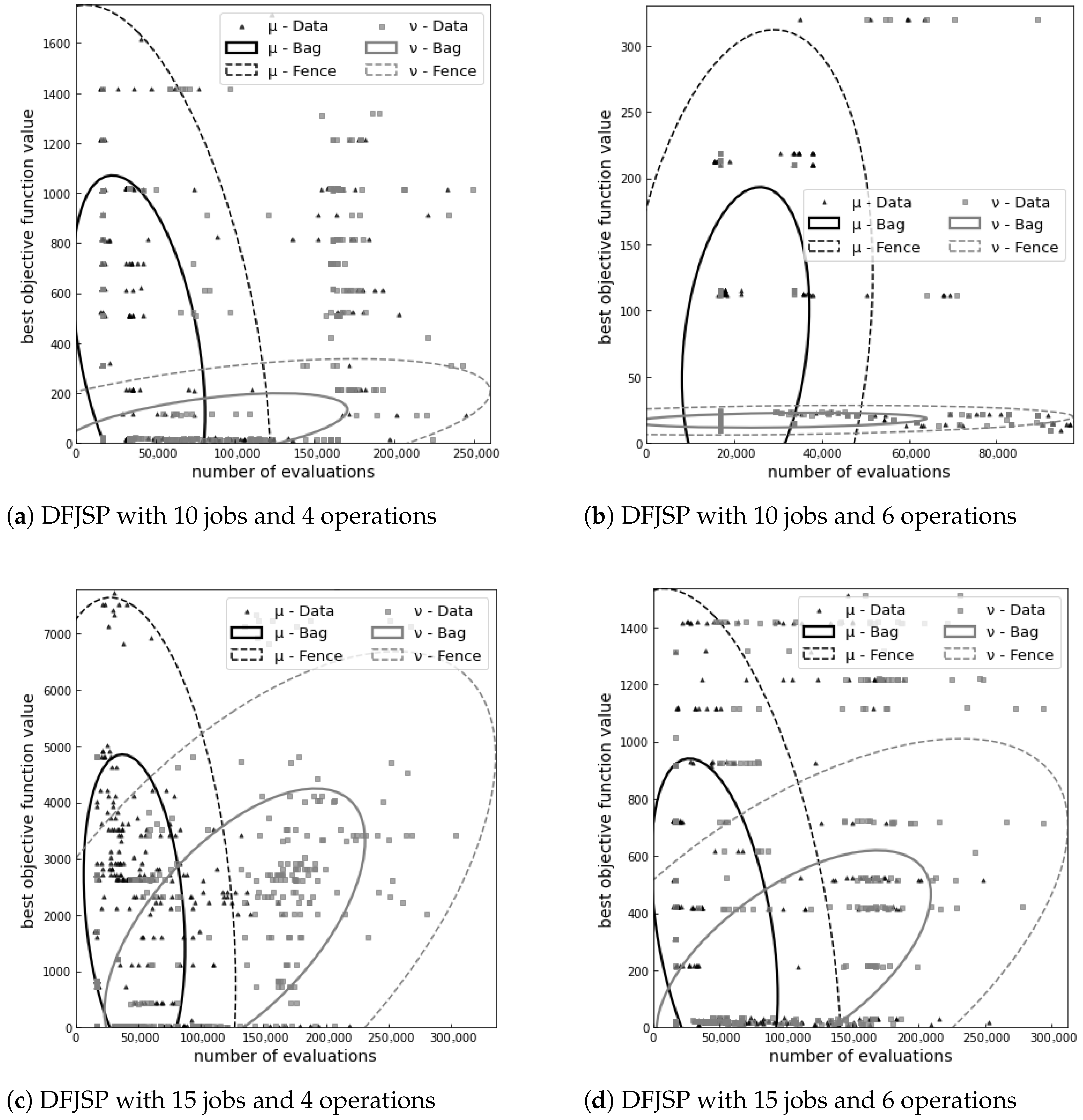
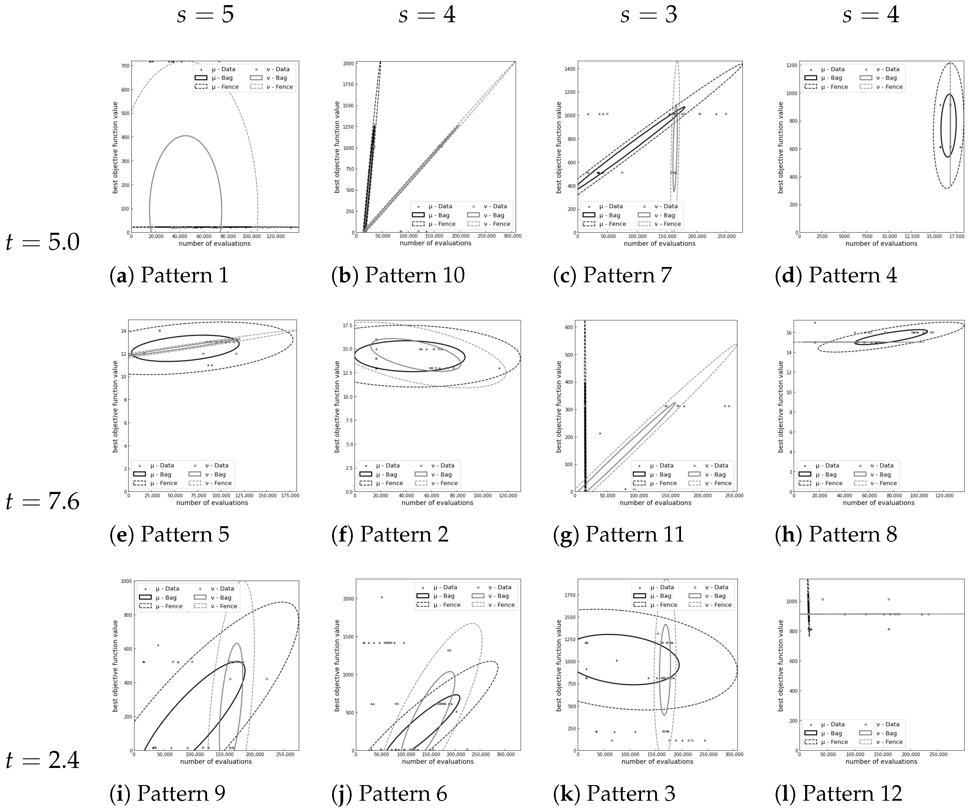
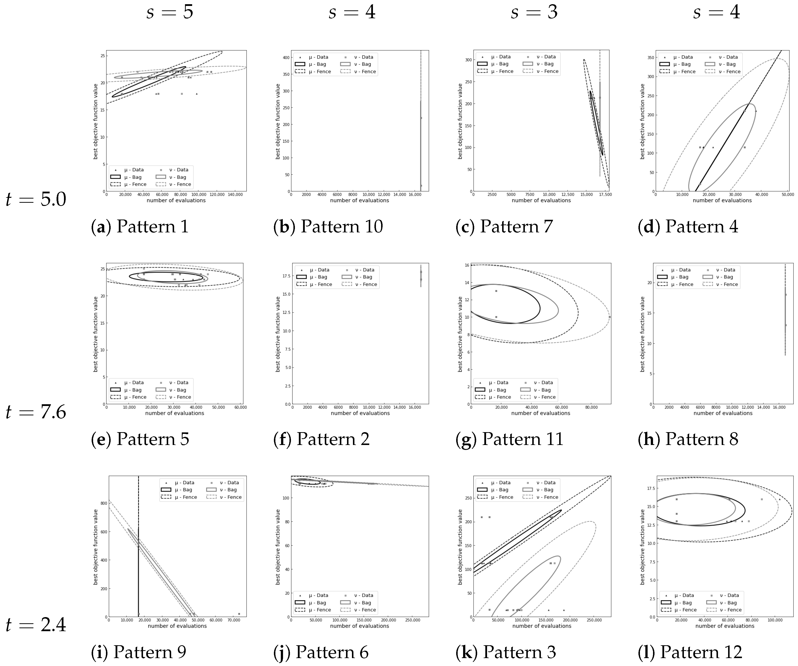
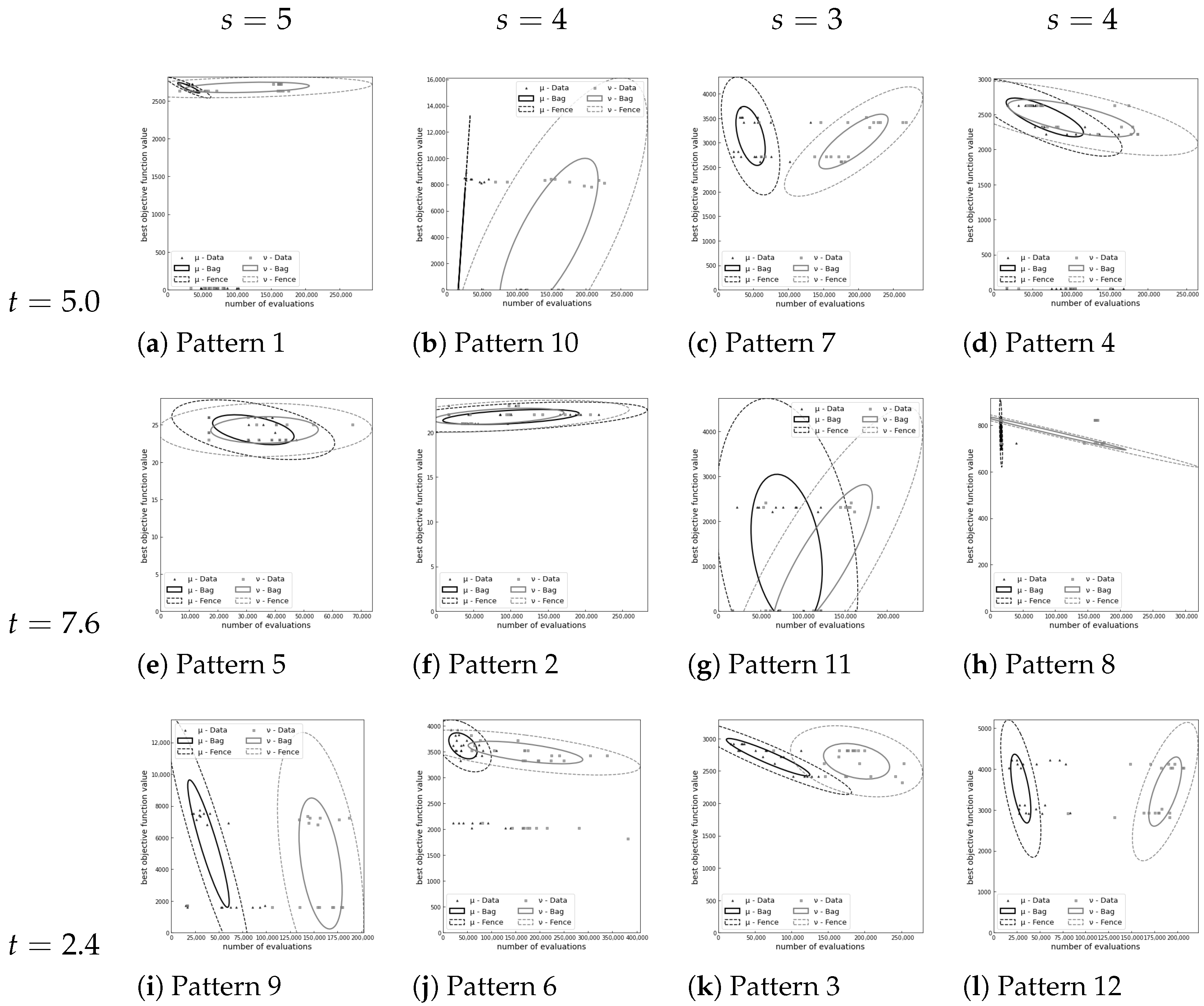
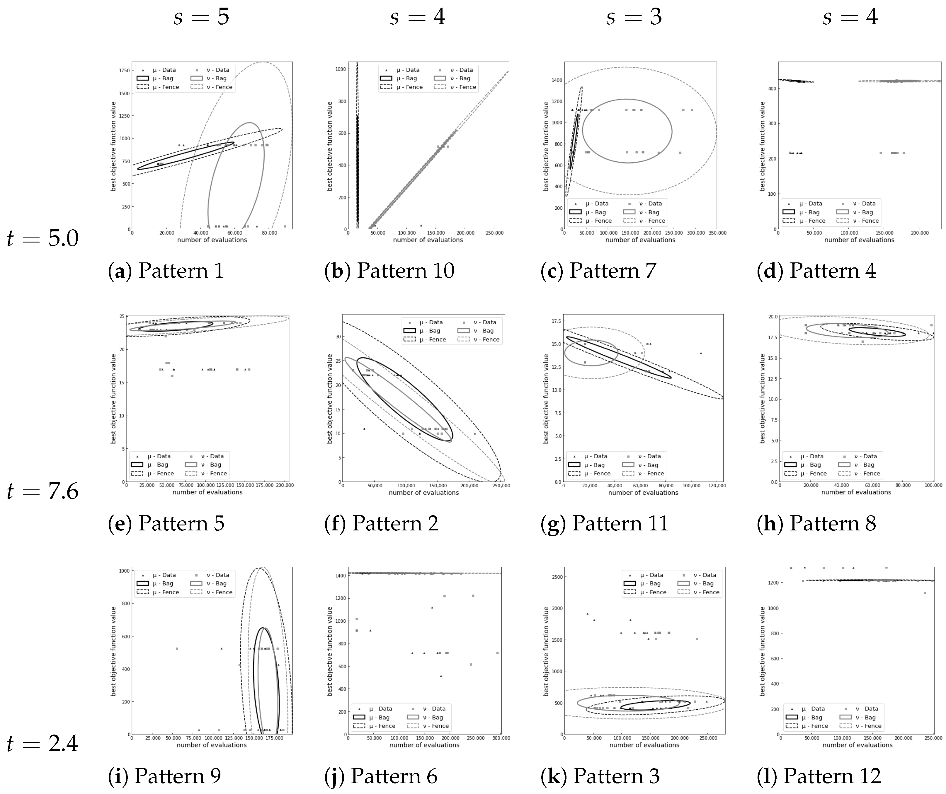
Figure 4 shows a Bagplot illustrating the relationship between the obtained best objective function values and the number of evaluations for each method. Here, the number of evaluations represents the frequency of creating a schedule using the DR obtained from an individual and calculating its fitness. Furthermore,
Figure 5,
Figure 6,
Figure 7 and
Figure 8 show the variations for each pattern of arriving job sets in the DFJSP. These figures present Bagplots categorized into 12 combinations of the maximum operation processing time
s and the due date tightness variable
t. A Bagplot visualizes the features of a data distribution by showing the central region and the range of outliers in two-dimensional data. The inner solid line indicates the central region containing the top 50% of data closest to the median, while the outer dotted line indicates the boundary for outliers, extending 1.5 times beyond the central region. The black lines represent the results for APF-GP-
, and the gray lines represent those for APF-GP-
.
From
Figure 4, it can be observed that APF-GP-
results in a larger number of evaluations and smaller objective values compared to APF-GP-
. Furthermore, while APF-GP-
tends to decrease the number of evaluations as the objective values increase, APF-GP-
tends to increase the number of evaluations as the objective values increase.
Figure 5,
Figure 6,
Figure 7 and
Figure 8 show that similar distributions are obtained regardless of whether APF-GP-
or APF-GP-
is used in cases where the range of objective values is small, such as in
Figure 5f,
Figure 6g,
Figure 7f and
Figure 8e. The variance in objective values is small when the due date tightness variable
t is 7.6, which makes tardiness less likely to occur. This variance is also small in
Figure 6, where the degree of freedom for operation selection is high relative to the given jobs. In contrast, in cases where the range of objective values is large, such as in
Figure 7i, APF-GP-
requires more evaluations than APF-GP-
. The range of objective values is large when the variable
t is 2.4, which makes tardiness more likely to occur. This range is also large in
Figure 5, where the degree of freedom for operation selection is low. It is observed that the larger the range of objective values, the greater the difference in the number of evaluations tends to be.
These results suggest that by using APF-GP-, the proposed method resolves the issue where APF-GP- fails to appropriately increase the population size when the range of objective values is large, which prevents sufficient solution search. Consequently, it can be concluded that the objective values were improved.
3.4. Experiments with Larger-Scale Scenarios
The scheduling problems presented in
Table 3 involve a relatively small number of operations. Therefore, it is necessary to verify whether consistent results can be obtained in larger scheduling problems involving jobs with more operations than those in the previous experiments. To this end, numerical experiments with 10 trials are conducted for the larger-scale scheduling problems shown in
Table 9.
The experimental results obtained using each method are shown in
Table 10.
Table 10 shows that APF-GP can reduce computation time even in complex scheduling problems with more operations. Comparing the performance within APF-GP, APF-GP-
achieves shorter computation time, while APF-GP-
yields better objective function values. These results are consistent with those obtained for the scheduling problems in
Table 3. This suggests that APF-GP remains effective for scheduling problems with a larger number of operations and that APF-GP-
can improve the objective function values compared to APF-GP-
.