Article

Genetic Programming with Adaptive Population Restructuring for Dynamic Flexible Job Shop Scheduling

Graduate School of Advanced Science and Engineering, Hiroshima University, Higashihiroshima 739-8527, Japan
*
Author to whom correspondence should be addressed.
Mathematics 2026, 14(6), 1000; https://doi.org/10.3390/math14061000
Submission received: 23 January 2026 / Revised: 6 March 2026 / Accepted: 12 March 2026 / Published: 16 March 2026
(This article belongs to the Special Issue Metaheuristic Algorithms, 2nd Edition)

Abstract

In the dynamic flexible job shop scheduling problem (DFJSP) where the environment changes irregularly, priority rules are used to calculate priorities for each job and machine, determining the processing order. To achieve efficient scheduling, it is necessary to select appropriate priority rules that match the problem’s characteristics whenever the environment changes. To address such problems, Genetic Programming (GP) has been proposed to derive mathematically expressed priority rules. Various GP-based methods exist, among which Population-based Fluctuation GP (PF-GP) is an efficient technique that reuses individuals adapted to problem characteristics. However, optimizing the DFJSP using PF-GP requires significant computational cost. Therefore, methods have been developed to adaptively change the population size for more efficient resource utilization. This paper modifies the adaptive population size change into a population growth method designed to balance scheduling performance and computational efficiency in the DFJSP. By applying this proposed method to various scheduling problems, this paper investigates its effectiveness. Furthermore, this paper compares population growth methods and demonstrates that the proposed method addresses conventional issues in existing population adjustment techniques, enabling the more efficient utilization of computational resources.

1. Introduction

A scheduling problem is a combinatorial optimization problem that determines the processing order of jobs and is applied to determining efficient production processes and work schedules. Among various scheduling problems, the dynamic flexible job shop scheduling problem (DFJSP) can model complex production processes involving environmental changes during the execution of the schedule, such as problem constraints and the set of jobs to be processed. Therefore, it maintains high fidelity to practical scheduling problems. In general, for dynamic scheduling problems, methods have been considered that assign priorities to each operation constituting a job using priority rules such as Dispatching Rules (DRs) and perform scheduling based on those priorities [1].
As a method for automatically generating priority rules, Genetic Programming (GP) [2], which can generate priority rules expressed as mathematical formulas through a tree structure, is superior to other priority rule generation methods because it can flexibly respond to dynamic environments and the resulting rules are highly interpretable [3]. Among various GP methods, such as Island GP (IGP) [3], which manages multiple populations to achieve both intensive search and individual diversity, and Population-Selection-based GP/IGP [4], which performs genetic operations by reusing preserved populations, Population-based Fluctuation GP (PF-GP) has been shown to perform efficient solution searches for dynamic scheduling problems [5]. PF-GP searches for solutions using a set of individuals selected from an environment where the number of populations fluctuates.
In the DFJSP, the computational cost is high because two types of rules are required: machine assignment and job selection. In general, the number of individuals required for an efficient solution search varies depending on the target problem. It has been shown that the computational efficiency of PF-GP can be improved by adaptively adjusting the population size [6] based on the concept of Population Resizing on Fitness Improvement GA (PRoFIGA) [7], which performs optimization while adjusting the number of individuals in the population according to changes in fitness.
In the DFJSP, the scale of the objective function to be optimized varies depending on the characteristics of the job sets, resulting in different magnitudes of fitness. However, conventional methods do not take this into account, and the judgment criteria for population size adjustment are not always appropriate, often leading to a failure to increase the population size adequately. To address this issue, this paper proposes a modification to accommodate varying fitness scales across different job sets. Furthermore, the effectiveness of the proposed method is verified through numerical experiments on various scheduling problems.
The structure of this paper is as follows. Section 2 introduces conventional research on the DFJSP and evolutionary computation methods, then proposes an improvement to PF-GP using an adaptive population. Section 3 conducts comparative experiments using the conventional and proposed methods to verify the usefulness of the proposed method. Finally, Section 4 provides the conclusion of this paper and discusses future work.

2. Materials and Methods

2.1. Dynamic Scheduling Problems

A dynamic scheduling problem is a type of problem where real-time events, such as the arrival of new job sets or machine failures, occur intermittently, requiring scheduling to be performed each time. Many practical scheduling problems are dynamic, involve complex relationships between operations and machines, and require the efficient execution of optimal scheduling. In the dynamic flexible job shop scheduling problem (DFJSP), there are multiple machines capable of processing a single operation. The processing order of operations for each job is predetermined, and two or more operations of the same job cannot be processed simultaneously. An operation is processed by only one machine at a time, each machine can process only one job at a time, and the processing of a job cannot be interrupted. Furthermore, this paper only considers the arrival of new job sets as the real-time event for the DFJSP. The variables related to the DFJSP are shown in Table 1.
In the DFJSP, each time a new job set arrives, the objective function E given by Equation (1) is used to evaluate the schedule. The evaluation is based on the weighted sum of the makespan C max d = max { C i d | i = 1 , 2 , , L d } , which is the total time required to process all unprocessed jobs, and the total tardiness i = 1 L d T i d .
minimize E = C max d + W T × i = 1 L d T i d
where W T is the weight for tardiness. Furthermore, each schedule is evaluated by the fitness F defined by Equation (2).
F = 1 E

2.2. Evolutionary Computation Methods and Scheduling Problems

2.2.1. Optimization of Dynamic Scheduling Problems Using GP

In the optimization of scheduling problems using Genetic Algorithms (GAs), the processing order of jobs and operations, as well as the machines to be used, is determined based on the priority held by each individual. On the other hand, when using GP, an individual represents a priority rule called a Dispatching Rule (DR) for determining priorities. For this reason, in dynamic scheduling problems, when a new job set arrives, the priorities can be determined using a previously acquired DR. GP is suitable for dynamic scheduling problems because it does not require the re-initialization of individuals every time a new job set arrives, as is the case when using GAs.
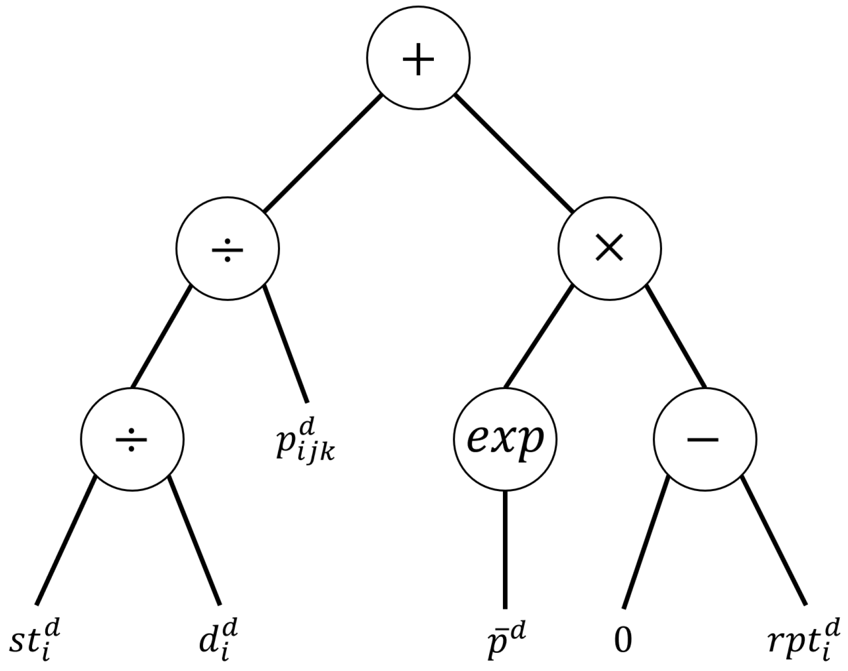
When using GP, each individual is represented by a tree structure, as shown in Figure 1, using nodes selected from terminal sets consisting of several indicators for jobs and operations and function sets consisting of arithmetic operations and selection functions.
The individual shown in Figure 1 represents the priority P I i j k of operation o i j d and the k-th capable machine, given by
P I i j k = s t i d / d i d p i j k d + exp { p ¯ d } · ( 0 r p t i d )
where processing is performed in descending order of priority. The DR is evaluated based on the objective function value in Equation (1) for the resulting schedule.
In GP, optimizing scheduling problems incurs higher computational costs as the problems become more complex; thus, various methods have been explored to mitigate these costs. F. Zhang et al. [8] achieved efficient exploration with a smaller population size by simultaneously evolving populations of different sizes, thereby utilizing DRs with distinct characteristics acquired by each population. X. Chen et al. [9] realized early convergence in multi-objective scheduling problems by concurrently evolving multiple populations, each focused on optimizing a single objective. Y. Mei et al. [10] achieved efficient exploration using a broad terminal set by adjusting the usage frequency of features based on their importance.
Furthermore, in dynamic scheduling problems, the optimal rule changes with the arrival of each job set. While it has been demonstrated that performing re-optimization upon job arrival can lead to more efficient results [11], few studies have focused on re-optimizing using GP. In most GP-based approaches, optimization is performed using a single acquired DR, which requires low computational cost but results in limited optimization performance. Therefore, it is necessary to develop methods that achieve efficient re-optimization by effectively utilizing previously acquired DRs during the subsequent search process.

2.2.2. Population Resizing on Fitness Improvement GA

In PRoFIGA [7], if the fitness is improved during the search process, a further improvement in the solution can be expected, and the population size is increased to improve the diversity of the population. If the fitness is not improved for a short period, an intensive search should be performed in the neighborhood of the individual with the best fitness, and the population size is then reduced by deleting a certain number of low-fitness individuals. If the fitness is not improved for a long period, the entire population is considered to have fallen into a local optimum, so the population size is increased. As described above, PRoFIGA is an algorithm that achieves efficient solution search by adaptively adjusting the population size based on changes in the scale of fitness.
Let F n e w d , F p r e d , and F i n i d be the fitness of the best individual in the current population, the fitness of the best individual in the previous generation during the evolutionary process, and the fitness of the best individual in the initial generation, respectively. When the maximum population size is P m a x and the current population size is P c u r d , the increase rate μ d of the population size used for the solution search at the d-th job set arrival, when PRoFIGA increases the number of individuals, is determined by Equation (4).
μ d = r · ( P m a x P c u r d ) · F n e w d F p r e d F i n i d , r ( 0 , 1 )
In PRoFIGA, the use of elitism in the reproduction process prevents a decrease in fitness in the subsequent generation, ensuring that Equation (4) does not take a negative value.
On the other hand, when decreasing the population size, the population size is multiplied by ( 1 ξ ) , where ξ ( 0 , 1 ) is the reduction coefficient.

2.2.3. Optimization of DFJSP Using GP

In the optimization of the DFJSP, a combination of a routing rule (RR), which selects a machine to process each operation, and a sequencing rule (SR), which determines the processing order of operations on each machine, must be selected. In the conventional DR generation framework using a tree structure, expressing both the RR and SR in a single tree structure leads to a complex structure, making solution search difficult [12]. To avoid such problems, several methods have been proposed, such as Cooperative Coevolution GP (CCGP) [13], which performs scheduling using a DR generated by combining individuals selected from two independently evolving populations corresponding to the RR and SR, and Multi-Tree GP (MTGP) [12], which uses individuals with two tree structures corresponding to the RR and SR.

2.3. PF-GP with Adaptive Population Resizing

Adaptive Population-based Fluctuation GP (APF-GP) [6], which incorporates the population resizing mechanism of PRoFIGA [7] into PF-GP [5] for the DFJSP, has achieved a moderate reduction in computational costs [6]. However, this reduction in APF-GP [6] is accompanied by a decline in solution performance. This paper aims to reduce computational costs while mitigating this performance degradation by improving the population resizing method of conventional APF-GP.

2.3.1. Overview of PF-GP

In PF-GP [5], each time a new job set arrives, two populations are chosen for genetic operations: one is the Selected population adapted to the characteristics of the job sets, and the other is the Base population used across all solution searches. The number of populations is adaptively adjusted based on the characteristics of the job set. If it is determined that no population fits the scheduling problem, a new population is generated, and genetic operations are performed on both this new population and the Base population. Furthermore, if multiple populations are judged to fit a job set with the same characteristics, they are integrated. As described above, PF-GP achieves efficient solution search by adjusting the number of populations.

2.3.2. Overview of APF-GP

APF-GP [6] adjusts the population size based on changes in the scale of fitness, similarly to PRoFIGA [7]. The increase rate of the population size is determined by Equation (4). However, if the total tardiness of the best individual in the current generation ( i = 1 L j T i ) n e w and that of the best individual in the previous generation during the evolutionary process ( i = 1 L j T i ) p r e are both zero (i.e., ( i = 1 L j T i ) n e w = ( i = 1 L j T i ) p r e = 0 ), the increase rate given by Equation (5) is used, where F p r e d is used instead of F i n i d .
μ d = r · ( P m a x P c u r d ) · F n e w d F p r e d F p r e d , r ( 0 , 1 )
By changing the increase rate to use only the fitness of the best individuals whose tardiness is zero, the population size can be adjusted while excluding the influence of tardiness, which has a minimum value of zero and cannot be improved further [6]. The change in the growth rate when switching from μ to μ falls within the expected range of variation observed when the fitness improves at the growth rate μ .

2.3.3. Revision of Population Resizing Rules

When using the increase rate μ d given by Equation (4), if the range of reachable fitness becomes narrow, the difference in fitness ( F n e w d F p r e d ) becomes smaller compared to F i n i d . Consequently, depending on the characteristics of the job set, it becomes difficult to increase the population size appropriately. For this reason, adjusting the increase rate μ d by Equation (4) is not necessarily appropriate for dynamic scheduling problems where the range of fitness can change significantly due to the arrival of new job sets. To address this issue, this paper uses the increase rate ν d given by Equation (6).
ν d = r · ( P m a x P c u r d ) · F n e w d F p r e d F n e w d F i n i d , r ( 0 , 1 )
By using the ratio of ( F n e w d F p r e d ) to the fitness difference ( F n e w d F i n i d ) , the influence of the scale of fitness can be reduced, and appropriate population resizing can be achieved. Even when the range of fitness becomes narrow, adjusting the computational cost based on the degree of improvement is expected to result in better DRs, although the computational costs may increase.
In this paper, let APF-GP using the growth rate μ d be defined as APF-GP- μ and APF-GP using the growth rate ν d be referred to as APF-GP- ν .

2.3.4. Reuse of Existing Populations

Compared to a newly and randomly generated population, reusing an existing population is expected to lead to the discovery of good solutions with less search effort, as it is considered to be fitted to some extent even for new job sets. For this reason, APF-GP deletes half of the individuals in a population through tournament selection [6]. This paper also adopts this population resizing mechanism.

2.3.5. The Structure of the Proposed Method

The algorithm of the proposed method is described below. Let N p be the initial population size for a newly generated population, N d be the number of Selected populations upon the arrival of the d-th job set, and N 0 be the number of initially Selected populations. Furthermore, the Base population is divided into two types: a Storage Base population for preserving obtained individuals and a Search Base population that selects individuals from the storage to be used in the solution search.
The fitting condition for individuals in a population is defined as W × α d , where W is a weight, and α d is a fitness criterion. This criterion α d is determined by the best objective function value obtained through a low-cost GP search on the current job set. In this low-cost search, the population size is set to N p / 10 , and the termination condition is defined as the state where the objective function value has not been updated for 10 consecutive generations. Threshold parameters β and γ are introduced to determine the suitability of population integration. Specifically, β is used to verify whether the data size is sufficient for the evaluation in Step 3-2-3, while γ assesses whether different populations are fitted to job sets with similar characteristics. Additionally, the population size is increased using δ when a solution stagnates for an extended period to prevent the search from falling into a local optimum.
Step 1 
Generate N p individuals for the Storage Base population and N 0 · N p individuals for the Selected population using the Ramped half-and-half method. Set d = 0 and proceed to Step 2.
Step 2 
When a new job set arrives, set d = d + 1 and proceed to Step 3.
Step 3 
If d N 0 , choose the d-th Selected population from those generated in Step 1 and proceed to Step 4-1. If d > N 0 , calculate the objective function values for all individuals against the unprocessed job set. A population is judged to fit the unprocessed job set if 10% or more of its individuals satisfy the fitting condition. Proceed to Step 3-1 if one population is judged as fitted, to Step 3-2 if multiple populations are fitted, and to Step 3-3 if zero populations are fitted.
Step 3-1 
Choose the population judged as fitted and proceed to Step 4-2.
Step 3-2 
 
Step 3-2-1 
Let p b e s t d be the population containing the individual with the smallest objective function value from Equation (1) among those judged as fitted, and let P d be the set of fitted populations excluding p b e s t d . Proceed to Step 3-2-2.
Step 3-2-2 
If P d , randomly select and remove one population p f i t d from P d , then proceed to Step 3-2-3. If P d = , choose population p b e s t d and proceed to Step 4-2.
Step 3-2-3 
Let d s t be the larger value between the arrival counts of the job sets when p b e s t d and p f i t d were respectively generated. If d d s t β , proceed to Step 3-2-4; otherwise, return to Step 3-2-2.
Step 3-2-4 
Let C m p b e s t d and C m p f i t d be the proportions of individuals satisfying the fitting condition for populations p b e s t d and p f i t d at each job set arrival from the d s t -th to the d-th arrival ( m = d s t , d s t 1 , , d ). If the correlation coefficient between C m p b e s t d and C m p f i t d is greater than or equal to γ , integrate the two populations p b e s t d and p f i t d using tournament selection. If it is less than γ , no integration is performed. Return to Step 3-2-2.
Step 3-3 
Generate a new population consisting of N p individuals, set it as the Selected population, increment the population count N d = N d + 1 , and proceed to Step 4-1.
Step 4 
 
Step 4-1 
Duplicate all individuals from the Storage Base population to form the Search Base population. Using these duplicated individuals and those in the Selected population as the initial population, proceed to Step 5.
Step 4-2 
Select N p / 2 individuals from the Storage Base population using roulette wheel selection based on the fitness Equation (2) to form the Search Base population. Similarly, select N p / 2 individuals from the Selected population via roulette wheel selection to serve as its initial individuals, and proceed to Step 5.
Step 5 
Perform genetic operations—reproduction, crossover, and mutation—independently on the Search Base population and the Selected population. For the reproduction operation within the Selected population, the individual with the highest fitness in the Search Base population is copied to replace one individual in the Selected population. Proceed to Step 6.
Step 6 
Compare the fitness of the current population with that of the previous generation. If the current fitness has improved, proceed to Step 6-1. If the fitness has stagnated without improvement and the number of stagnated generations exceeds δ , proceed to Step 6-1. If the number of stagnated generations is δ or fewer, proceed to Step 6-2.
Step 6-1 
If the tardiness of the best individuals in the current and previous generations is non-zero, increase the number of individuals using the increase rates μ d and ν d . If the tardiness of both best individuals is zero, increase the number of individuals using the rate μ d . When increasing the population size, new individuals are generated using the Ramped half-and-half method. Proceed to Step 7.
Step 6-2 
Reduce the number of individuals used for the solution search by setting the reproduction size to ( 1 ξ ) times the original size. Proceed to Step 7.
Step 7 
If the termination condition is met, randomly select up to N p / 2 unique individuals from the Search Base population and replace individuals in the Storage Base population such that its total size becomes N p . For the Selected population, store all individuals from the search process and return to Step 2. If the termination condition is not met, return to Step 5.
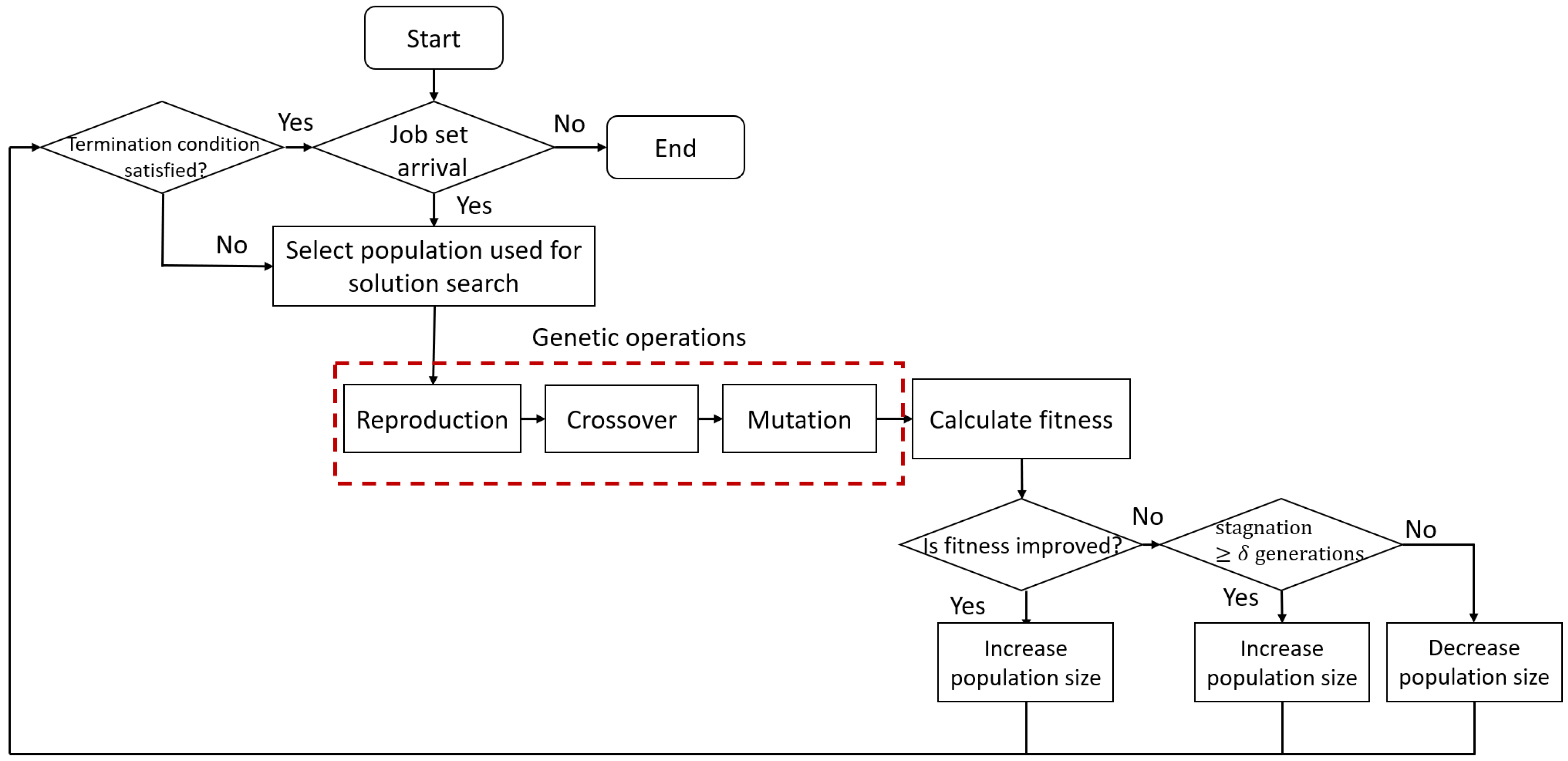
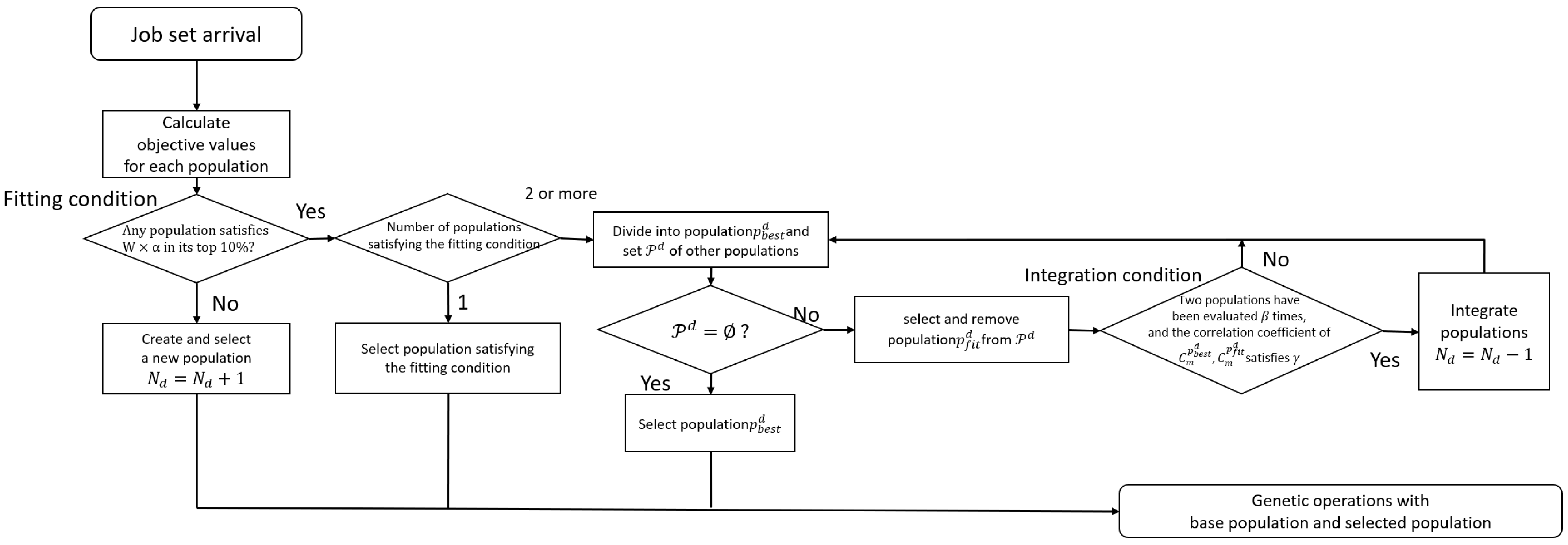
The overall flowchart of the proposed method is shown in Figure 2, and the flowchart for population selection is shown in Figure 3.

2.3.6. Parameter Tuning Methodology

APF-GP utilizes parameters W , β , and γ related to the behavior of the number of populations, as well as parameters r , ξ , and δ governing the adjustment of population size. Each parameter significantly impacts exploration performance and computational costs; therefore, careful design is required according to the specific problem being addressed. This section provides guidelines for tuning these parameters.
By tuning the parameters related to the behavior of the number of populations, the adaptability to the characteristics of job sets is determined. A larger value of W makes the existing populations more likely to be judged as adapted. Since the excessive generation of new populations consumes significant computational costs, it is crucial to adjust W such that it is not excessively small. A larger value of β allows for the integration judgment to be made by considering a larger amount of data. This parameter should be adjusted according to constraints on computational costs and the expected frequency of rescheduling. γ represents the threshold for the correlation coefficient; it is generally desirable to use a value of 0.7 or higher, which indicates a strong positive correlation.
By tuning the parameters related to the behavior of population size adjustment, the degree of increase and decrease in the number of individuals within a population is determined. The parameters r and ξ adjust the growth and reduction rates of the population size, respectively. In this paper, these were tuned with reference to [7,14]. For r, the growth rate must be appropriately adjusted based on the maximum population size and the magnitude of fitness values. By tuning the parameters related to the behavior of population size adjustment, the degree of increase and decrease in the number of individuals within a population is determined. A larger value of δ extends the number of generations during which the population size can be reduced, thereby enabling an intensive search over a longer period. Conversely, if δ is set too small, APF-GP tends to increase the population size more frequently, which diminishes the expected reduction in computational cost. Therefore, δ should be adjusted in accordance with time constraints and the number of search iterations.

3. Results

In this section, numerical experiments are conducted on the DFJSP using GP, PF-GP [5], APF-GP- μ [6], and APF-GP- ν to verify the effectiveness of the proposed method.

3.1. Experimental Setup

R T d is determined by the weighted sum of the arrival time of the ( d 1 ) -th job set and the makespan C max d of the schedule created by adding the d-th job set, as shown in Equation (7):
R T d = R T d 1 + 0.8 × C max d , R T 0 = 0
In the experiments, the number of job set arrivals is set to 30, and the d-th job set is assumed to arrive at time R T d . This experimental setup is adopted to generate new job sets, representing dynamic changes, only after the previously scheduled processing has sufficiently progressed. This allows for the evaluation of both the performance of the generated schedules and the capability to respond to dynamic changes. The number of jobs in each set is defined as the number of jobs whose operations were all completed between the arrival of the previous job set and the arrival of the new one.
The number of machines capable of processing each operation, m i j d , and the index of these machines, d m i j k , are determined as follows, where a 1 and a 2 are uniform random numbers in the range [ 0 , 1 ) , and M is the total number of machines available simultaneously:
m i j d = a 1 M + 1 , m i j d Z
d m i j k d = a 2 M + 1 , m i j k d m i j k d , m i j k d Z
In this experiment, a scenario is considered where the characteristics of the arriving job sets vary with a cycle of 12. This is achieved by varying the maximum operation processing time s and the variable t, which determines the tightness of due dates, with cycles of 4 and 3, respectively, upon each job set arrival, as described below:
s : 5 4 3 4 5 4
t : 5.0 7.6 2.4 5.0 7.6 2.4
This approach can reproduce the scheduling of orders and production with mid-to-long-term cycles—such as seasonal patterns and market trends observed in actual production sites—as well as weekly and monthly production plans. Therefore, this paper conducts simulations using job sets possessing periodic characteristics. The processing time p i j k d of the operations of job i in the newly arriving d-th job set, the ready time (earliest start time) s t i d , and the due date d i d are determined using uniform random numbers a 3 , a 4 , a 5 [ 0 , 1 ] as follows:
p i j k d = a 3 ( s 1 ) + 1
s t i d = a 4 p ¯ d + s t j d
d i d = s t i d + p ¯ d ( 1 + a 5 t )
Each individual in GP uses the representation format of MTGP [12]. For each generation, scheduling is performed using the best individual. If the objective function value E obtained from the scheduling has not been improved for 30 consecutive generations during the search process, the solution is interpreted to have converged, and the search is terminated. The parameters used in this experiment are shown in Table 2.
The experiments were conducted on a computer equipped with an 11th Gen Intel(R) Core(TM) i7-11700 processor, 16.0 GB RAM, and Intel(R) UHD Graphics 750. The software environment consisted of Windows 11, Python 3.10.9, and NumPy 1.25.2.

3.2. Numerical Results

To compare GP [2], PF-GP [5], APF-GP- μ [6], and APF-GP- ν , ten trial runs were conducted for the scheduling problems with the number of jobs and operations shown in Table 3.
Table 4, Table 5, Table 6 and Table 7 show the experimental results for each method, including the average objective function value, the average makespan C max , the total tardiness of all jobs T i , the computation time, and the average total number of generations across ten trials. These tables also provide a comparison of the average objective function values between the proposed method and conventional GP and PF-GP. Wilcoxon rank-sum tests were performed at a significance level of 5%. In the comparison results, “+” indicates that the objective function value is significantly larger (worse) than the comparative target, “−” indicates that it is significantly smaller (better), and “≈” indicates no significant difference. Additionally, Table 8 shows the ratio of the computation time for each scenario relative to that of PF-GP.
From Table 4, Table 5, Table 6 and Table 7, in Scenarios (10, 4), (10, 6), and (15, 6), PF-GP achieves better objective values than GP with approximately the same computation time. While APF-GP- μ and APF-GP- ν show worse objective values than PF-GP, they substantially reduce the computation time. Furthermore, APF-GP- μ requires less computation time, whereas APF-GP- ν provides better objective values.
Focusing solely on the objective values, PF-GP is significantly better than GP in Scenarios (10, 4) and (10, 6). While APF-GP- μ is significantly worse than PF-GP in Scenarios (10, 6) and (15, 6), APF-GP- ν is significantly worse only in Scenario (10, 6). In Scenario (10, 6), the objective function value obtained by APF-GP is inferior to that of PF-GP. This is because, in Scenario (10, 6), cases where tardiness occurs—which is heavily weighted and prioritized in Equation (1)—are rare, and the makespan accounts for a larger proportion of the objective function value. APF-GP evaluates the increase in population size based on the degree of improvement in the objective function. Consequently, improvements in makespan, which have a smaller impact on the overall value, are given lower priority, leading the algorithm to prioritize reducing computational time in such cases. Therefore, it is considered that APF-GP prioritized computational time more than in other scenarios, resulting in objective function values significantly worse than those of PF-GP in Scenario (10, 6). Furthermore, when no tardiness occurs, the increase rate is switched to μ . This explains why the differences in objective function values and computational times between APF-GP- μ and APF-GP- ν are smaller. These results suggest that APF-GP- μ is more appropriate for scheduling in environments like Scenario (10, 6), where tardiness is unlikely to occur and the objective is to reduce computational time.
As shown in Table 8, compared to PF-GP, APF-GP- μ drastically reduces the computation time to approximately 35– 55 % , and APF-GP- ν reduces it to approximately 50– 75 % .

3.3. Analysis of Population Increase Rates

To compare APF-GP- μ and APF-GP- ν , the relationship between the objective values and the number of evaluations for each scheduling task is analyzed. In the experiments in this section, to strictly compare the optimization results of the scheduling for each job set arrival, an experimental setup is employed where the state of the remaining jobs at the time of each job set arrival is kept identical. Specifically, to synchronize the uncompleted jobs at the time a new job set arrives, pre-processing is performed on the jobs based on a common rule obtained via PF-GP. A situation is set where a new job set arrives during this process. Subsequently, all uncompleted jobs, including the newly arrived ones, are rescheduled according to the same pre-defined rules. The repetition of this operation clarifies the performance difference between the two methods. This procedure standardizes the influence of remaining jobs across all trials at the time of a job set arrival, making it ideal for analyzing the impact of each individual arrival.
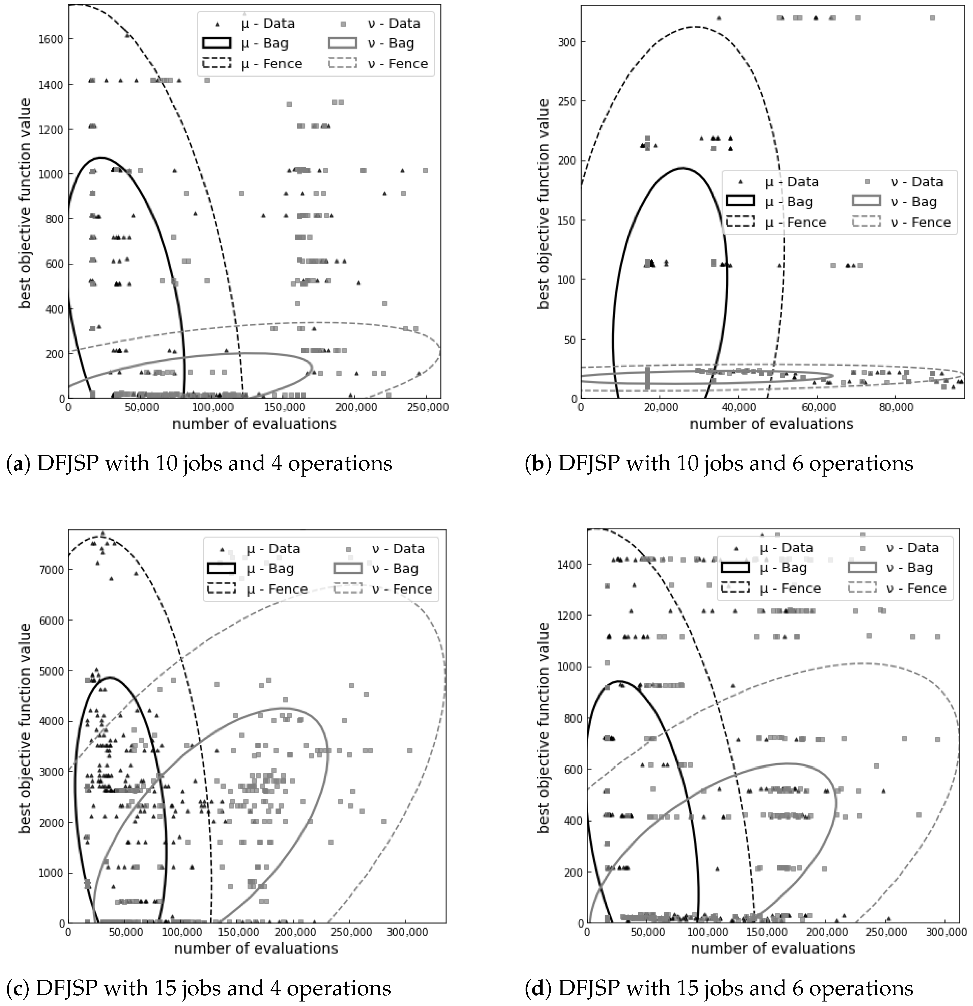
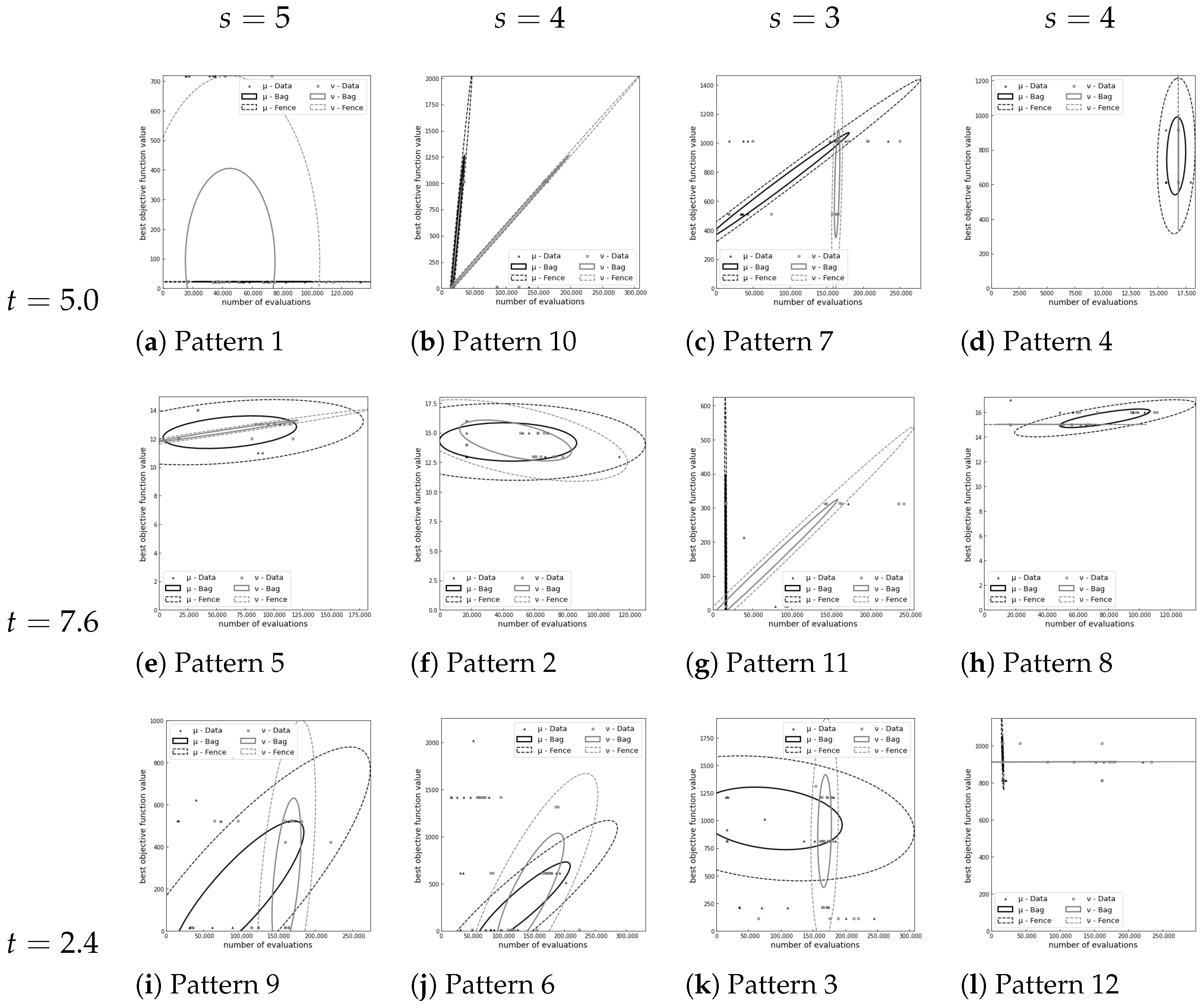
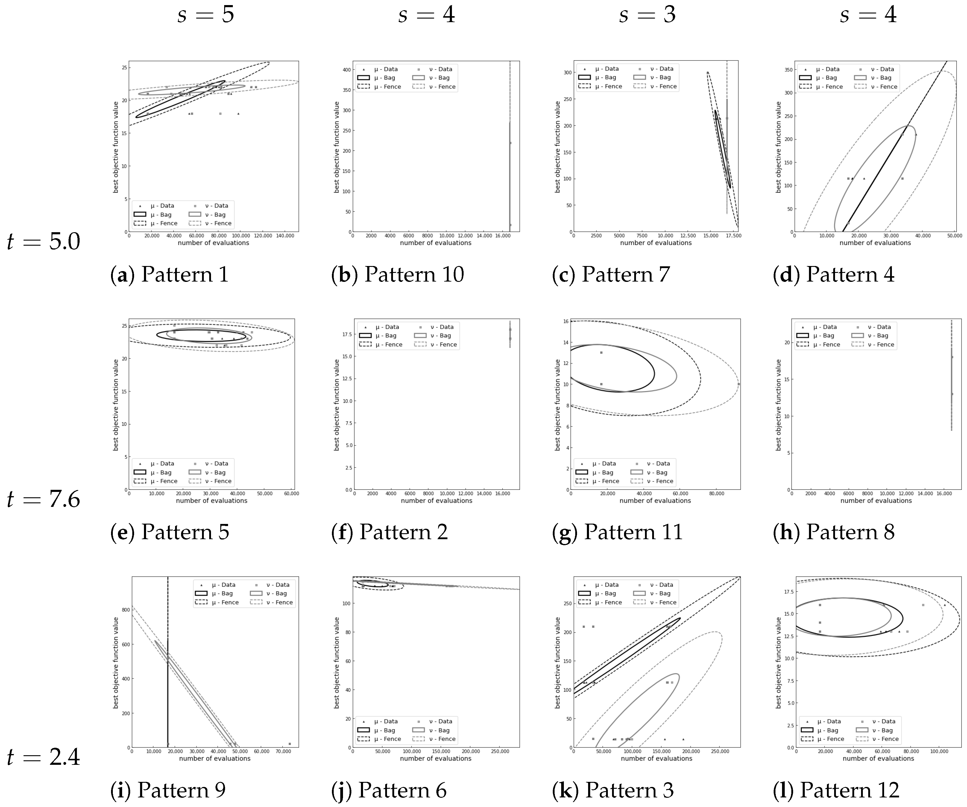
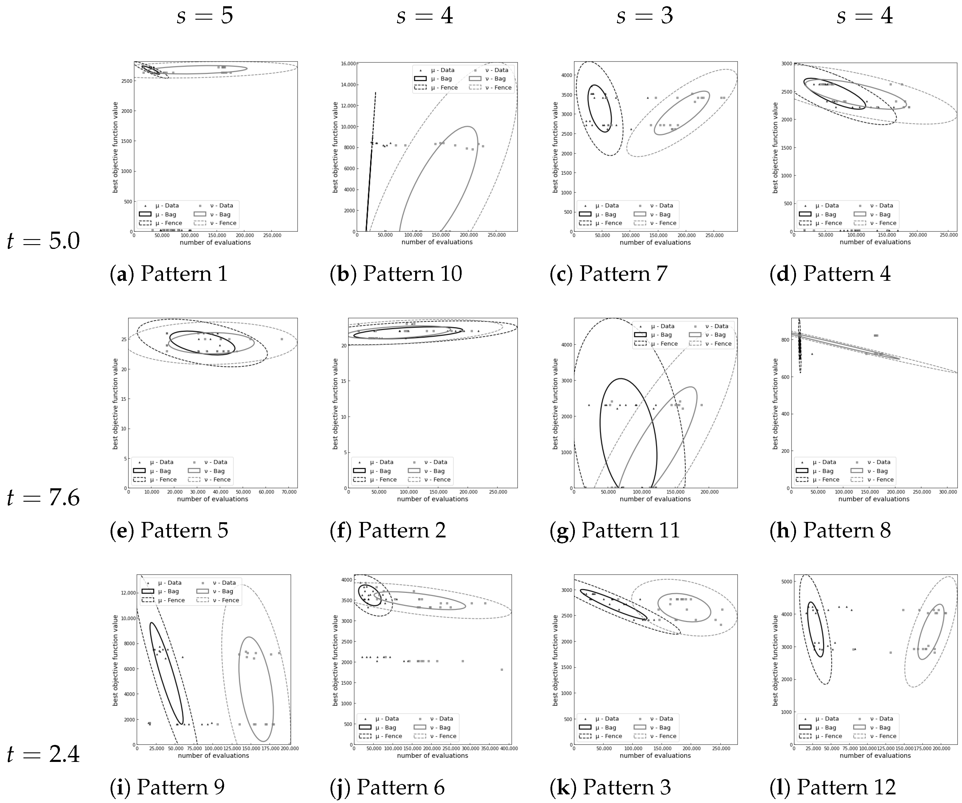
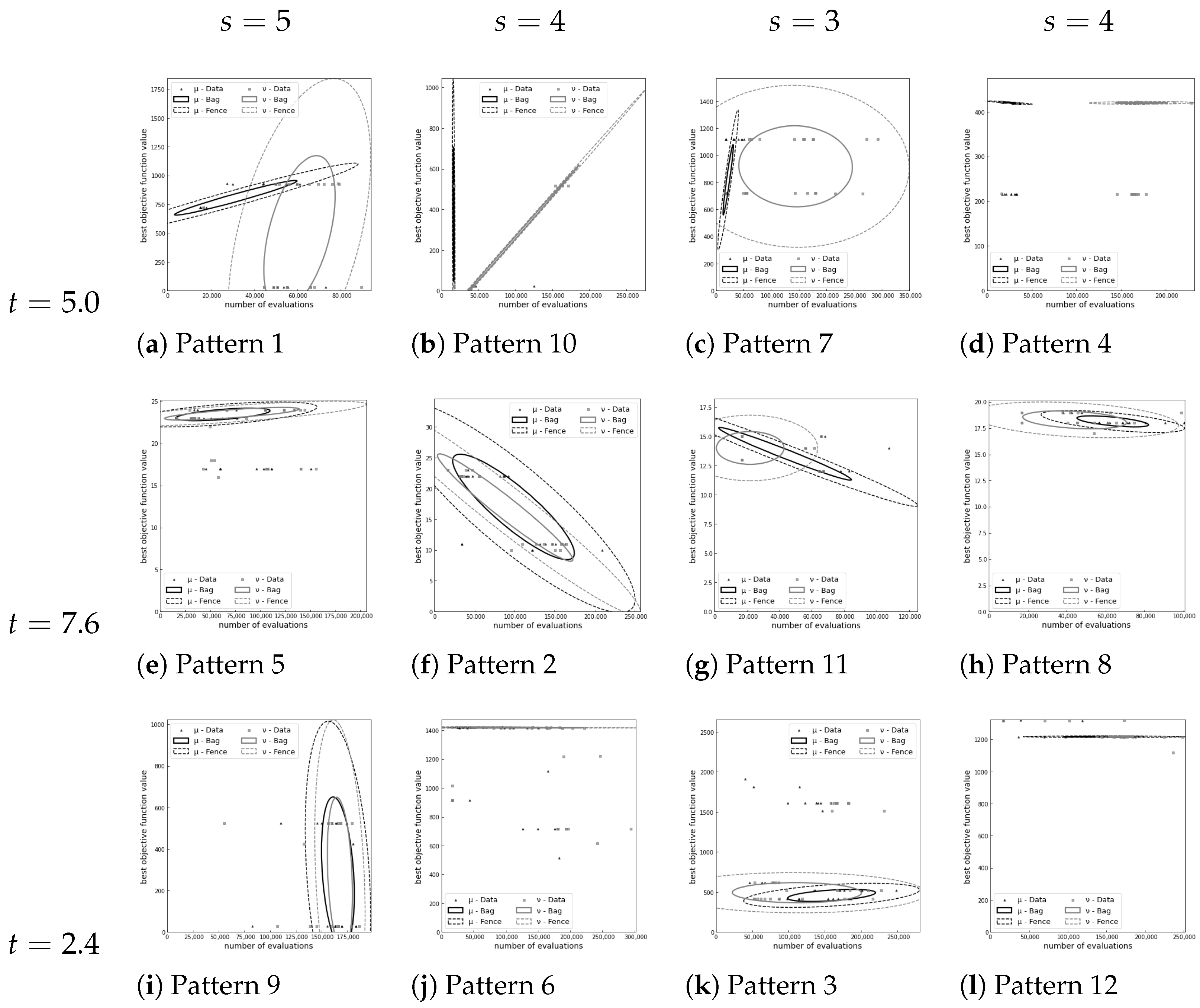
Ten trial runs were conducted for the scheduling problems given in Table 3. Figure 4 shows a Bagplot illustrating the relationship between the obtained best objective function values and the number of evaluations for each method. Here, the number of evaluations represents the frequency of creating a schedule using the DR obtained from an individual and calculating its fitness. Furthermore, Figure 5, Figure 6, Figure 7 and Figure 8 show the variations for each pattern of arriving job sets in the DFJSP. These figures present Bagplots categorized into 12 combinations of the maximum operation processing time s and the due date tightness variable t. A Bagplot visualizes the features of a data distribution by showing the central region and the range of outliers in two-dimensional data. The inner solid line indicates the central region containing the top 50% of data closest to the median, while the outer dotted line indicates the boundary for outliers, extending 1.5 times beyond the central region. The black lines represent the results for APF-GP- μ , and the gray lines represent those for APF-GP- ν .
From Figure 4, it can be observed that APF-GP- ν results in a larger number of evaluations and smaller objective values compared to APF-GP- μ . Furthermore, while APF-GP- μ tends to decrease the number of evaluations as the objective values increase, APF-GP- ν tends to increase the number of evaluations as the objective values increase.
Figure 5, Figure 6, Figure 7 and Figure 8 show that similar distributions are obtained regardless of whether APF-GP- μ or APF-GP- ν is used in cases where the range of objective values is small, such as in Figure 5f, Figure 6g, Figure 7f and Figure 8e. The variance in objective values is small when the due date tightness variable t is 7.6, which makes tardiness less likely to occur. This variance is also small in Figure 6, where the degree of freedom for operation selection is high relative to the given jobs. In contrast, in cases where the range of objective values is large, such as in Figure 7i, APF-GP- ν requires more evaluations than APF-GP- μ . The range of objective values is large when the variable t is 2.4, which makes tardiness more likely to occur. This range is also large in Figure 5, where the degree of freedom for operation selection is low. It is observed that the larger the range of objective values, the greater the difference in the number of evaluations tends to be.
These results suggest that by using APF-GP- ν , the proposed method resolves the issue where APF-GP- μ fails to appropriately increase the population size when the range of objective values is large, which prevents sufficient solution search. Consequently, it can be concluded that the objective values were improved.

3.4. Experiments with Larger-Scale Scenarios

The scheduling problems presented in Table 3 involve a relatively small number of operations. Therefore, it is necessary to verify whether consistent results can be obtained in larger scheduling problems involving jobs with more operations than those in the previous experiments. To this end, numerical experiments with 10 trials are conducted for the larger-scale scheduling problems shown in Table 9.
The experimental results obtained using each method are shown in Table 10.
Table 10 shows that APF-GP can reduce computation time even in complex scheduling problems with more operations. Comparing the performance within APF-GP, APF-GP- μ achieves shorter computation time, while APF-GP- ν yields better objective function values. These results are consistent with those obtained for the scheduling problems in Table 3. This suggests that APF-GP remains effective for scheduling problems with a larger number of operations and that APF-GP- ν can improve the objective function values compared to APF-GP- μ .

4. Discussion

This paper verifies the effectiveness of APF-GP, a variant of PF-GP that adjusts the population size during the search based on the PRoFIGA concept, through numerical experiments using multiple dynamic flexible job shop scheduling problems. The results demonstrated that APF-GP reduced computational costs compared to conventional methods: to approximately 35– 55 % for APF-GP- μ and 50– 75 % for APF-GP- ν . Furthermore, the employment of APF-GP- ν successfully addresses the issue in APF-GP- μ where the number of evaluations becomes excessively small when the fitness range is narrow. This confirms that APF-GP- ν enables evaluations with an appropriate count tailored to the complexity of the scheduling problem. However, in scenarios with small objective function values, APF-GP- ν does not improve search performance, suggesting that APF-GP- μ is preferable in such cases. Consequently, APF-GP- μ is superior when prioritizing a further reduction in computational costs or when dealing with scenarios featuring small objective function values. In contrast, APF-GP- ν is suitable for complex problems where maintaining optimization performance while achieving time reductions is required.
Future work should include a more detailed analysis of the characteristics associated with different increase rates, conducting experiments in larger-scale scenarios, verifying reproducibility and stability, performing comparative evaluations with other GP-based variants, and establishing a methodology for parameter tuning.

Author Contributions

Conceptualization, T.H.; methodology, M.U. and S.S.; software, M.U.; validation, T.H., and S.S.; data curation, M.U.; writing—original draft preparation, M.U.; writing—review and editing, T.H.; supervision, T.H. and S.S.; project administration, T.H. All authors have read and agreed to the published version of the manuscript.

Funding

This research received no external funding.

Data Availability Statement

The original contributions presented in this study are included in the article. Further inquiries can be directed to the corresponding author.

Conflicts of Interest

The authors declare no conflicts of interest.

References

  1. Kaweegitbundit, P.; Eguchi, T. Flexible job shop scheduling using genetic algorithm and heuristic rules. J. Adv. Mech. Des. Syst. Manuf. 2016, 10, 1–18. [Google Scholar] [CrossRef] [Scilit]
  2. Koza, J.R.; Rice, J.P. Genetic Programming: The Movie; MIT Press: Cambridge, MA, USA, 1992. [Google Scholar]
  3. Hayashida, T.; Nishizaki, I.; Sekizaki, S.; Mochida, H. Development of an island model distributed genetic algorithm with different evolutionary rules. IEEJ Trans. Electron. Inf. Syst. 2021, 141, 1430–1436. [Google Scholar]
  4. Hayashida, T.; Hirotani, D.; Nishizaki, I.; Sekizaki, S.; Maeda, I. Parallel distributed genetic programming using long-term memory for dynamic scheduling problems. Trans. Inst. Syst. Control Inf. Eng. 2022, 35, 93–100. [Google Scholar]
  5. Urabe, M.; Hayashida, T.; Sekizaki, S.; Nishizaki, I. Improvement of population-adjustment genetic programming for dynamic scheduling problems. In Proceedings of the 2024 IEEE SMC Hiroshima Chapter Workshop for Young Researchers, Hiroshima, Japan; IEEE: Piscataway, NJ, USA, 2024; pp. 1–8. [Google Scholar]
  6. Urabe, M.; Hayashida, T.; Sekizaki, S. Proposal of genetic programming with adaptive structural population change for dynamic scheduling problems. In Proceedings of the 2025 IEEE SMC Hiroshima Chapter Workshop for Young Researchers, Hiroshima, Japan; IEEE: Piscataway, NJ, USA, 2025; pp. 5–10. [Google Scholar]
  7. Eiben, A.E.; Marchiori, E.; Valko, V.A. Evolutionary algorithms with on-the-fly population size adjustment. In Parallel Problem Solving from Nature—PPSN VII, Proceedings of the 7th International Conference, Granada, Spain; Springer: Berlin/Heidelberg, Germany, 2004; Volume 7, pp. 41–50. [Google Scholar]
  8. Zhang, F.; Mei, Y.; Nguyen, S.; Zhang, M. Collaborative Multifidelity-Based Surrogate Models for Genetic Programming in Dynamic Flexible Job Shop Scheduling. IEEE Trans. Cybern. 2022, 52, 8142–8156. [Google Scholar] [CrossRef] [Scilit] [PubMed]
  9. Chen, X.; Li, J.; Wang, Z.; Chen, Q.; Gao, K.; Pan, Q. Optimizing Dynamic Flexible Job Shop Scheduling Using an Evolutionary Multi-Task Optimization Framework and Genetic Programming. IEEE Trans. Evol. Comput. 2025, 29, 1502–1516. [Google Scholar] [CrossRef] [Scilit]
  10. Mei, Y.; Nguyen, S.; Xue, B.; Zhang, M. An Efficient Feature Selection Algorithm for Evolving Job Shop Scheduling Rules With Genetic Programming. IEEE Trans. Emerg. Top. Comput. Intell. 2017, 1, 339–353. [Google Scholar] [CrossRef] [Scilit]
  11. Shen, X.N.; Yao, X. Mathematical modeling and multi-objective evolutionary algorithms applied to dynamic flexible job shop scheduling problems. Inf. Sci. 2015, 298, 198–224. [Google Scholar] [CrossRef] [Scilit]
  12. Zhang, F.; Mei, Y.; Zhang, M. Genetic programming with multi-tree representation for dynamic flexible job shop scheduling. In Proceedings of AI 2018: Advances in Artificial Intelligence, Sydney, Australia; Springer: Cham, Switzerland, 2018; pp. 472–484. [Google Scholar]
  13. Yska, D.; Mei, Y.; Zhang, M. Genetic programming hyper-heuristic with cooperative coevolution for dynamic flexible job shop scheduling. In Genetic Programming, Proceedings of the 21st European Conference, EuroGP 2018, Parma, Italy; Springer: Cham, Switzerland, 2018; pp. 306–321. [Google Scholar]
  14. Rajakumar, B.R.; George, A. APOGA: An Adaptive Population Pool Size based Genetic Algorithm. AASRI Procedia 2013, 4, 288–296. [Google Scholar] [CrossRef] [Scilit]
Figure 1. An example of an individual in GP.
Mathematics 14 01000 g001
Figure 2. Flowchart of proposed method.
Mathematics 14 01000 g002
Figure 3. Flowchart of population selection with population resizing.
Mathematics 14 01000 g003
Figure 4. Bagplots showing the relationship between the number of evaluations and best objective function value.
Mathematics 14 01000 g004
Figure 5. Bagplots for each job arrival pattern in Scenario (10, 4).
Mathematics 14 01000 g005
Figure 6. Bagplots for each job arrival pattern in Scenario (10, 6).
Mathematics 14 01000 g006
Figure 7. Bagplots for each job arrival pattern in Scenario (15, 4).
Mathematics 14 01000 g007
Figure 8. Bagplots for each job arrival pattern in Scenario (15, 6).
Mathematics 14 01000 g008
Table 1. The variables related to the DFJSP.
MNumber of machines
dNumber of job set arrivals
L d Number of jobs at the d-th job set arrival
J i d i-th job at the d-th job set arrival ( i = 1 , 2 , , L d )
N i d Number of operations of J i d
o i j d j-th operation of J i d ( j = 1 , 2 , , N i d )
m i j d Number of machines capable of processing o i j d
d m i j k d k-th machine capable of processing o i j d ( k = 1 , 2 , , m i j d )
p i j k d Processing time of o i j d on machine d m i j k d
s t j d Arrival time of the d-th job set
s t i d Ready time of J i d
d i d Due date of J i d
C d Completion time of J i d
T d Tardiness of J i d
r p n i d Number of remaining operations of J i d
r p t i d Remaining processing time of J i d
p ¯ d Average processing time per job in the d-th job set
n i q i j k Number of waiting operations at machine d m i j k d
m w t i j k Total processing time of waiting operations at machine d m i j k d
w i q i j k Current processing stage of the job at machine d m i j k d
Table 2. Parameters of PF-GP.
ParameterValue
Initial number of populations6 (including Base population)
Maximum number of populations25 (including Base population)
Crossover probability0.8
Mutation probability0.1
Selection methodRoulette wheel selection, elitism
Initial individual generationRamped half-and-half method
Maximum tree depth8
Terminal set for routing rules4 types ( n i q i j k , w i q i j k , m w t i j k , p i j k d )
Terminal set for sequencing rules8 types ( p i j k d , p ¯ d , d i d , s t i d , r p t i j d , r p n i j d , 1 , 0 )
Function set6 types ( + , , × , / , max , exp )
β 5
γ 0.7
δ 10
W1.5
Maximum population size7500
Minimum population size100
Increase rate adjustment parameter r0.1
Population reduction parameter ξ 20 %
Table 3. The scenarios of the scheduling problems used in the experiments.
Scenario(10, 4)(10, 6)(15, 4)(15, 6)
Number of jobs in each set1015
Number of operations per job4646
Number of machines4646
Table 4. Experimental results for Scenario (10, 4).
MethodObjective Values C max T i Time [s]Total GenerationsSig. Diff. (GP)Sig. Diff. (PF-GP)
GP 244.4 14.77 2.30 11,6071024 +
PF-GP 226.3 14.60 2.12 11,5481011
APF-GP- μ 234.7 14.73 2.20 6459988
APF-GP- ν 227.0 14.66 2.12 7761995
Table 5. Experimental results for Scenario (10, 6).
MethodObjective Values C max T i Time [s]Total GenerationsSig. Diff. (GP)Sig. Diff. (PF-GP)
GP 66.0 16.37 0.50 14,299929 +
PF-GP 63.6 16.31 0.47 14,791920
APF-GP- μ 66.4 16.39 0.50 5570881+
APF-GP- ν 66.1 16.39 0.50 7334889+
Table 6. Experimental results for Scenario (15, 4).
MethodObjective Values C max T i Time [s]Total GenerationsSig. Diff. (GP)Sig. Diff. (PF-GP)
GP 1104.9 20.88 10.84 24,8981206
PF-GP 1154.3 20.96 11.33 25,4431227
APF-GP- μ 1210.3 21.31 11.89 99161144+
APF-GP- ν 1116.9 20.93 10.96 18,0441171
Table 7. Experimental results for Scenario (15, 6).
MethodObjective Values C max T i Time [s]Total GenerationsSig. Diff. (GP)Sig. Diff. (PF-GP)
GP 333.3 18.97 3.14 32,3421122
PF-GP 322.3 18.92 3.03 34,2511106
APF-GP- μ 343.6 19.30 3.24 15,6631092+
APF-GP- ν 325.4 19.10 3.06 25,6031095
Table 8. Computation time ratio relative to PF-GP for each scenario (%).
Scenario(10, 4)(10, 6)(15, 4)(15, 6)
PF-GP 100.0 100.0 100.0 100.0
APF-GP- μ 55.9 37.7 39.0 45.7
APF-GP- ν 67.2 49.6 70.9 74.8
Table 9. Scenarios of larger-scale scheduling problems used in experiments.
Scenario(10, 10)
Number of jobs in each set10
Number of operations per job10
Number of machines4
Table 10. Experimental results for Scenario (10, 10).
MethodObjective Values C max T i Time [s]Total GenerationsSig. Diff. (GP)Sig. Diff. (PF-GP)
GP 525.6 32.0 4.94 33,4161240
PF-GP 536.4 32.0 5.04 34,5171238
APF-GP- μ 552.8 32.4 5.20 14,2761175+
APF-GP- ν 539.8 32.2 5.08 22,4941171
Disclaimer/Publisher’s Note: The statements, opinions and data contained in all publications are solely those of the individual author(s) and contributor(s) and not of MDPI and/or the editor(s). MDPI and/or the editor(s) disclaim responsibility for any injury to people or property resulting from any ideas, methods, instructions or products referred to in the content.