Adaptive Ensemble Weight Optimization for Natural Gas Consumption Forecasting: A Hybrid Stochastic–Deep Learning Framework Applied to the Czech Market

Abstract

The transition towards data-driven energy management requires predictive frameworks capable of handling the nonlinear and non-stationary nature of natural gas consumption. Traditional static models often struggle to adapt to rapid regime shifts in liberalized markets. To address this forecasting problem, this study proposes a convex ensemble weight optimization framework. Moving beyond simple model averaging, we formulate the ensemble weighting problem as a constrained convex optimization task on the unit simplex. We utilize the Frank–Wolfe algorithm (Conditional Gradient) to dynamically optimize the weights of a heterogeneous set of base learners, including SARIMAX, XGBoost, N-HiTS, and Temporal Fusion Transformers (TFTs). Our results on the Czech gas market dataset demonstrate that this mathematically grounded approach achieves a Mean Absolute Percentage Error (MAPE) of 4.25%, which compares favorably to individual models such as N-HiTS (5.31%) and static averaging (6.74%). While the accuracy gain over greedy ensemble selection is marginal, the proposed convex formulation offers improved stability and interpretability, which are practical advantages for operational deployment.

1. Introduction

Accurate forecasting of natural gas consumption is an essential element of energy security and economic efficiency, particularly in countries with high import dependence and seasonal demand variability, such as the Czech Republic. The liberalization of energy markets has encouraged data-driven decision-making, where the ability to predict daily demand fluctuations directly impacts the financial stability of market participants [1]. In the context of recent European energy market fluctuations and the transition to renewable sources, the volatility of consumption patterns has increased, rendering traditional static forecasting models insufficient [2]. As noted by [3], static models struggle to capture concept drift in residential consumption, creating a need for adaptive forecasting frameworks.

The current literature focuses heavily on the development of complex individual architectures, ranging from Gradient Boosting Machines (GBMs) [4,5] to Recurrent Neural Networks (RNNs) [6]. However, the “No Free Lunch” theorem implies that no single model is universally superior across all temporal regimes. While ensemble learning offers a pathway to mitigate this limitation [7], standard approaches often rely on simple averaging or heuristic meta-learners that lack theoretical convergence guarantees.

This paper addresses this gap by shifting the research focus from the development of individual predictors to the operational research problem of optimal forecast combination. The primary hypothesis of this study is that the daily prediction task can be modeled as a decision-making process where a meta-learner dynamically assigns weights to a portfolio of diverse algorithms. Formulating this problem as a constrained convex optimization task on the unit simplex provides regularization that enhances stability compared to unconstrained or greedy approaches.

Unlike black-box stacking methods, this proposed framework provides mathematical transparency, with the derived weights reflecting the instantaneous reliability of each base learner. This formulation bridges the gap between data-driven machine learning ensembles and the constraint satisfaction techniques of operations research. By mapping the forecasting problem onto the unit simplex, we substitute heuristic tuning with geometrical convergence guarantees.

The contribution of this study is threefold:

• Mathematical Formulation: We frame the ensemble weighting problem as a constrained convex optimization task on a simplex, minimizing a regularized loss function that reflects the asymmetry of balancing costs [8].
• Algorithmic Solution: We apply the Frank–Wolfe algorithm [9] and Ensemble Selection methods [10] to solve this optimization problem efficiently in a rolling window production environment.
• Empirical Validation: We provide a comprehensive validation on real-world Czech gas consumption data. We conduct an ablation study to quantify the contribution of each ensemble component and justify the choice of hyperparameters based on the physical properties of the natural gas market.

The remainder of this paper is organized as follows: Section 2 reviews the literature and identifies a research gap in the development of theoretically grounded ensemble methods. Section 3 details the proposed methodology and provides physical justifications for the chosen parameters. Section 4 presents the empirical results, including an ablation study. Section 5 discusses the operational implications, including computational complexity, and Section 6 concludes this work.

2. Literature Review

The forecasting of energy consumption has experienced a gradual transition from traditional econometric approaches to artificial intelligence methods. This section reviews the evolution of these methodologies, summarizing their contributions and limitations in the context of natural gas markets. To provide a precise positioning of our work, we present a comparative analysis of related approaches in Table 1.

2.1. Statistical and Econometric Models

Historically, statistical linear models such as ARIMA and its seasonal variants (SARIMAX) were the industry standard. However, forecasting natural gas consumption involves capturing complex nonlinear dependencies on meteorological factors, which linear models often fail to address adequately. Methods such as Multivariate Adaptive Regression Splines (MARS) have been proposed to better handle these nonlinearities than traditional regression [2]. Additive models like Prophet have also been employed successfully to model distinct multiple seasonalities and holiday effects [11], while smoothed physical variables are often utilized in statistical distributions [12].

2.2. Tree-Based Ensemble Methods and Machine Learning Approaches

To address the limitations of linear models, machine learning algorithms gained prominence. Gradient boosting frameworks (such as XGBoost) became highly popular due to their sparsity awareness and scalability for tabular data [4]. Random Forests have also demonstrated effectiveness for short-term load forecasting, showing a degree of resilience to non-stationarity [13]. Other studies have leveraged large-scale smart meter data mining to improve these models [14].

2.3. Classical Machine Learning

Beyond tree-based models, classical machine learning methods remain relevant for energy forecasting due to their interpretability and steady performance under limited data conditions. Support Vector Regression (SVR) and regularized linear models (such as ElasticNet) are frequently utilized to prevent overfitting in highly dimensional feature spaces where input variables are strongly correlated.

2.4. Deep Learning Architectures

In recent years, deep learning has offered strong results for complex time series. Long Short-Term Memory (LSTM) networks are widely used to model temporal sequences [6]. More recently, Transformer-based architectures have drawn attention. The Temporal Fusion Transformer (TFT) [15] introduces a multi-head attention mechanism combined with variable selection networks. Another notable development is N-HiTS [16], which reduces computational complexity using hierarchical blocks. Hybrid approaches, combining tree-based ensembles with deep learning, have also shown promising accuracy [17,18].

2.5. Ensemble Learning Taxonomy

Ensemble methods generally fall into three categories [19]: Bagging/Boosting (e.g., XGBoost [4]), Meta-Learning/Stacking [20], and Convex Weight Optimization. While Bagging and Stacking are powerful, they often lack interpretability. Our work adopts Convex Weight Optimization, using the Frank–Wolfe algorithm to dynamically optimize weights over the unit simplex.

It is important to note that optimization algorithms have found broader applications in machine learning beyond simple weighting. Techniques such as Genetic Algorithms (GAs) and Particle Swarm Optimization (PSO) have been extensively used for feature selection and hyperparameter tuning in energy forecasting [2]. However, these meta-heuristic approaches often lack convergence guarantees and require tuning of their own parameters. In contrast, convex optimization methods, such as the Frank–Wolfe algorithm used in this study, offer theoretical guarantees of convergence to a global optimum for convex objectives [9].

Table 1. Comparative analysis of related works in energy forecasting.

Category	References	Methodology	Key Advantages	Limitations
Statistical Models	Taylor and Letham [11]	Prophet (Additive Model)	Handles missing data, outliers, and holidays well.	Fails to capture complex nonlinear interactions.
	Smajla et al. [12]	Statistical Distribution Analysis	Effective use of smoothed temperature ($T_{eff}$).	Limited by simplified physical assumptions.
	Özmen [2]	MARS, CMARS	Modeling of nonlinearities in gas consumption.	Computational complexity in high dimensions.
	Box et al. [21]	ARIMA/SARIMAX	Theoretical interpretability, seasonality handling.	Linear assumption limits accuracy in volatile markets.
Tree-Based ML	Chen and Guestrin [4]	XGBoost	Scalability, sparsity awareness.	Requires extensive hyperparameter tuning.
	Svoboda et al. [14]	Smart Meter Data Mining	Insights from large-scale granular data collection.	Requires high-quality, dense historical data.
	Dudek [13]	Random Forest	Resilient to overfitting, handles non-stationarity.	Poor extrapolation outside training range.
Classical ML	Sharma et al. [22]	SVR, KNN, and other classical ML	Stable performance under limited data, strong interpretability.	Struggles with extreme nonlinearities compared to Deep Learning.
Deep Learning	Lim et al. [15]	Temporal Fusion Transformers	Interpretable attention mechanisms, multi-horizon.	High computational resource requirements.
	Zhao et al. [17]	Hybrid EL-VMD-Transformer	High accuracy by combining ensembles and DL.	Complex architecture, hard to deploy operationally.
	Panapakidis and Dagoumas [18]	Wavelet + GA-ANFIS	Hybrid approach handling signal non-stationarity.	High complexity of the multi-stage pipeline.
	Li and Sun [20]	EMLP (Adaptive MLP)	Adaptive weight correction within NN ensemble.	Weights optimized heuristically, not globally convex.
Ensemble Modelling	Marziali et al. [23]	Countrywide Ensembling	Proves ensembles outperform base learners (Italy).	Limited to standard averaging or simple regression.
	Liu et al. [24]	STL-based Hybrid Ensemble	Integrates STL decomposition with bagging for multi-scale price forecasting.	Univariate dataset, ignores exogenous factors (weather) and nonlinear meta-learners.
	Caruana et al. [10]	Ensemble Selection	Greedy optimization, creates reliable ensembles.	Can get stuck in local optima.
	This Study	Convex Optimization (FW)	Global convergence, sparsity, projection-free.	Requires convexity of the loss function.

Table 1. Comparative analysis of related works in energy forecasting.

Category	References	Methodology	Key Advantages	Limitations
Statistical Models	Taylor and Letham [11]	Prophet (Additive Model)	Handles missing data, outliers, and holidays well.	Fails to capture complex nonlinear interactions.
	Smajla et al. [12]	Statistical Distribution Analysis	Effective use of smoothed temperature ($T_{eff}$).	Limited by simplified physical assumptions.
	Özmen [2]	MARS, CMARS	Modeling of nonlinearities in gas consumption.	Computational complexity in high dimensions.
	Box et al. [21]	ARIMA/SARIMAX	Theoretical interpretability, seasonality handling.	Linear assumption limits accuracy in volatile markets.
Tree-Based ML	Chen and Guestrin [4]	XGBoost	Scalability, sparsity awareness.	Requires extensive hyperparameter tuning.
	Svoboda et al. [14]	Smart Meter Data Mining	Insights from large-scale granular data collection.	Requires high-quality, dense historical data.
	Dudek [13]	Random Forest	Resilient to overfitting, handles non-stationarity.	Poor extrapolation outside training range.
Classical ML	Sharma et al. [22]	SVR, KNN, and other classical ML	Stable performance under limited data, strong interpretability.	Struggles with extreme nonlinearities compared to Deep Learning.
Deep Learning	Lim et al. [15]	Temporal Fusion Transformers	Interpretable attention mechanisms, multi-horizon.	High computational resource requirements.
	Zhao et al. [17]	Hybrid EL-VMD-Transformer	High accuracy by combining ensembles and DL.	Complex architecture, hard to deploy operationally.
	Panapakidis and Dagoumas [18]	Wavelet + GA-ANFIS	Hybrid approach handling signal non-stationarity.	High complexity of the multi-stage pipeline.
	Li and Sun [20]	EMLP (Adaptive MLP)	Adaptive weight correction within NN ensemble.	Weights optimized heuristically, not globally convex.
Ensemble Modelling	Marziali et al. [23]	Countrywide Ensembling	Proves ensembles outperform base learners (Italy).	Limited to standard averaging or simple regression.
	Liu et al. [24]	STL-based Hybrid Ensemble	Integrates STL decomposition with bagging for multi-scale price forecasting.	Univariate dataset, ignores exogenous factors (weather) and nonlinear meta-learners.
	Caruana et al. [10]	Ensemble Selection	Greedy optimization, creates reliable ensembles.	Can get stuck in local optima.
	This Study	Convex Optimization (FW)	Global convergence, sparsity, projection-free.	Requires convexity of the loss function.

Recent hybrid approaches, such as the EL-VMD-Transformer-ResLSTM proposed by [17], demonstrate that combining tree-based ensembles with deep learning yields strong results. Similarly, ref. [23] confirmed, using Italian data, that ensemble strategies consistently outperform individual predictors.

Despite the efficacy of individual models, the “No Free Lunch” theorem suggests that no single model performs best under all conditions. As illustrated in Table 1, a gap exists in current methodologies. While deep learning models (TFT; N-HiTS) offer high accuracy, they suffer from opacity and high resource demands. Conversely, statistical models offer interpretability but lack the capacity to model complex nonlinearities. Most existing ensemble approaches rely on heuristic weighting or greedy selection, which do not guarantee global optimality.

Our study proposes a convex optimization framework that mathematically combines the diverse strengths of these base learners. By guaranteeing convergence on the unit simplex, we offer a solution that is interpretable and performs well, addressing the limitations identified in prior works.

3. Materials and Methods

To address the non-stationarity of gas consumption, we propose a modular ensemble framework. This structure ensures a clear separation between prediction generation, temporal adaptation, and weight optimization.

3.1. Layer 1: Base Learners (The Prediction Pool)

The first layer consists of a heterogeneous library of 15 algorithms. Diversity is necessary for ensemble success. Therefore, we deliberately selected models with distinct inductive biases. The complete set of base learners follows the established taxonomy.

3.1.1. Applied Statistical and Econometric Models

To ensure the ensemble is grounded in established statistical theory, we included the following:

• SARIMAX: The Seasonal AutoRegressive Integrated Moving Average with exogenous factors explicitly models seasonal components and the impact of external variables, such as temperature. Version of statsmodels used 0.14.6.
• ARX (Robust): An AutoRegressive model with exogenous variables focusing purely on linear dependencies between past consumption and current weather drivers. Version of statsmodels used 0.14.6.
• Prophet: An additive regression model that is reliable against missing data and shifts in the trend. Version of prophet used 1.2.1.

3.1.2. Applied Tree-Based Ensemble Methods and Machine Learning Approaches

Gradient boosting decision trees are highly effective for tabular data. We employed four distinct implementations to maximize diversity:

• XGBoost: A scalable implementation of gradient boosting that utilizes a sparsity-aware algorithm. Version of xgboost used 2.1.3.
• LightGBM: A gradient boosting framework designed to be efficient, utilizing a leaf-wise growth strategy. Version of lightgbm used 4.6.0.
• CatBoost: A high-performance library employing ordered boosting to overcome prediction shift [25]. Version of catboost used 1.2.8.
• ExtraTrees: A bagging method similar to Random Forest but with more randomness in the split selection to reduce variance. Version of scikit-learn used 1.8.

3.1.3. Applied Classical Machine Learning

We diversified the pool with classical regression and instance-based algorithms:

• Support Vector Regression (SVR): Effective in high-dimensional spaces and less prone to overfitting. Version of scikit-learn used 1.8.
• K-Nearest Neighbors (KNN): A nonparametric method predicting consumption based on the average of the k most similar historical days in the feature space. Version of scikit-learn used 1.8.
• ElasticNet: A linear regression model combining $L_1$ and $L_2$ priors. Version of scikit-learn used 1.8.
• Bayesian Ridge: A probabilistic approach introducing a prior probability distribution over the model parameters. Version of scikit-learn used 1.8.

3.1.4. Applied Deep Learning Architectures

Neural networks are employed to capture complex, nonlinear temporal dependencies:

• Temporal Fusion Transformers (TFTs): An attention-based architecture that combines high-performance multi-horizon forecasting with insights into temporal dynamics. Versions of libraries used: pytorch-lightning 2.6.0 and pytorch-forecasting 1.5.0.
• N-HiTS: A model that solves the forecasting problem using multi-rate signal sampling and hierarchical interpolation. Versions of libraries used: pytorch-lightning 2.6.0 and pytorch-forecasting 1.5.0.
• Long Short-Term Memory (LSTM): A recurrent neural network utilizing stacked layers to model the sequential nature of gas demand. Versions of libraries used: pytorch-lightning 2.6.0 and pytorch-forecasting 1.5.0.
• NeuralProphet: A hybrid framework combining the interpretability of statistical models with the scalability of deep learning. Version of neuralprophet used 0.9.0.

Each model i generates an independent forecast ${\widehat{y}}_{i,t}$.

3.2. Layer 2: Temporal Weighting Strategy

The second layer constitutes the adaptive memory of the system, addressing the challenge of concept drift where the statistical properties of the target variable change over time. In energy markets, such shifts are frequent due to seasonality or sudden meteorological events. Standard ensemble methods often assume that all historical data points are equally relevant (${\omega }_t=1$), leading to slow adaptation.

To mitigate this, we introduce a temporal weighting mechanism directly into the convex optimization objective in Equation (1). The objective minimizes a weighted sum of losses over the historical window H, prioritizing recent observations. Formally, the constrained optimization problem is defined by the objective function in Equation (1a), subject to the simplex constraints defined in Equation (1b,1c)

$$\begin{array}{cc}\hfill & \underset{w}{min}J\left(w\right)=\sum _{t=1}^H{\omega }_t·\mathcal{L}\left(y_t,\sum _{i=1}^N{w}_i{\widehat{y}}_{i,t}\right)\hfill \end{array}$$

(1a)

$$\begin{array}{cc}\hfill & \mathrm{s}.\mathrm{t}.\sum _{i=1}^N{w}_i=1,\hfill \end{array}$$

(1b)

$$\begin{array}{cc}\hfill & w_i\ge 0(w\in {\Delta }_N)\hfill \end{array}$$

(1c)

where $w={[w_1,\dots ,w_N]}^T$ is the vector of weights for the N base learners, and $J\left(w\right)$ represents the global cost function. The parameter H denotes the length of the historical training window, while ${\omega }_t$ assigns a temporal importance weight to each observation t. The term $\mathcal{L}(y_t,{\widehat{y}}_{ens,t})$ is the convex loss function. Finally, the constraints ensure the solution lies on the unit simplex.

We evaluate two distinct weighting kernels:

• Exponential Decay: A continuous forgetting factor defined as ${\omega }_t={\lambda }^{H-t}$, where $\lambda \in (0,1]$. This method can sometimes be overly aggressive in discarding useful information.
• Recency-Weighted Heuristic: Observations $t\in T_{recent}$ (the most recent week) are assigned a weight ${\omega }_t=3$, while older observations retain ${\omega }_t=1$.

The utilization of the weighting factor is based on the meteorological dynamics of Central Europe. Synoptic weather systems typically persist for 3 to 5 days. By weighting the most recent week more heavily, the model captures the inertia of the current weather regime. This approximates a Bayesian prior in which the current regime is three times as informative as the climatological average. The weighting factor ${\omega }_{high}=3$ is adopted as an expert-standard value based on domain knowledge from a Czech energy company. This value was obtained after a set of experiments with different values of ${\omega }_{high}$.

3.3. Layer 3: Ensemble Optimizer (Frank–Wolfe)

The third layer solves the constrained convex optimization problem to find the optimal weight vector w. We employ the Frank–Wolfe (Conditional Gradient) algorithm [26], a projection-free first-order optimization method. The choice of Frank–Wolfe over Projected Gradient Descent (PGD) is driven by two theoretical advantages:

• Computational Efficiency: In standard PGD, every iteration requires a projection onto the probability simplex ${\Delta }_N$ with complexity $\mathcal{O}(NlogN)$. Frank–Wolfe replaces this with a Linear Minimization Oracle (LMO), which reduces the complexity to $\mathcal{O}\left(N\right)$.
• Sparsity of Solutions: Frank–Wolfe updates the solution by iteratively moving towards a vertex of the simplex. This property naturally encourages sparsity, selecting a compact subset of the most relevant models.

The procedure is outlined in Algorithm 1.

To evaluate the practical utility of the proposed optimization, we benchmark the Frank–Wolfe approach against three established alternative strategies. These methods were deliberately selected to represent different methodological approaches to the forecast combination problem, specifically exact analytical solving, discrete greedy search, and online learning:

• Non-Negative Least Squares (NNLS): This method provides an exact analytical solution to the prediction problem by minimizing the squared error subject only to non-negativity constraints. While it mathematically guarantees the lowest error on the training window, it lacks structural regularization. This often leads to overfitting in noisy environments, distinguishing it from the iterative, sparsity-inducing procedure of Frank–Wolfe.
• Ensemble Selection (Greedy Optimization): A standard discrete heuristic proposed by [10]. Instead of calculating continuous weights, this algorithm iteratively adds the model that minimizes the ensemble’s overall error to the active pool. It serves as a highly effective baseline that avoids complex quadratic programming, though its greedy nature may cause it to settle in local minima and produce abrupt weight changes.
• Contextual Bandits (LinUCB): To contrast our batch-based rolling window approach with an online learning paradigm, we implemented a Linear Upper Confidence Bound (LinUCB) algorithm. This agent selects a single model at each time step based on the current meteorological context, treating forecast errors as negative rewards. This comparison tests whether immediate, context-aware selection is preferable to continuous portfolio weighting.

Algorithm 1 Frank–Wolfe for Ensemble Weights Optimization

Require:       Inputs:       1: Matrix of predictions $P\in {\mathbb{R}}^{H\times N}$       2: Vector of actual values $y\in {\mathbb{R}}^H$       3: Sample weights $\omega \in {\mathbb{R}}^H$       Parameters:       1: K: Number of iterations (set to 500)       2: $ϵ$: Tolerance parameter Ensure: Optimized weight vector $w^{\left(K\right)}\in {\Delta }_N$   1: Initialization: Set uniform weights $w^{\left(0\right)}\leftarrow {[1/N,\dots ,1/N]}^T$   2: for  $k=0,1,\dots ,K-1$  do   3:     Compute gradient $\nabla f\left(w^{\left(k\right)}\right)$ based on weighted loss   4:     Linear Minimization Oracle (LMO): Find vertex $s^{\left(k\right)}$ with the smallest gradient:   5:         $s^{\left(k\right)}\leftarrow arg{min}_{s\in {\Delta }_N}\langle s,\nabla f\left(w^{\left(k\right)}\right)\rangle$   6:     Calculate step size: $\gamma \leftarrow {\displaystyle \frac{2}{k+2}}$   7:     Update weights: $w^{(k+1)}\leftarrow (1-\gamma )w^{\left(k\right)}+\gamma s^{\left(k\right)}$   8:  end for   9:  return  $w^{\left(K\right)}$

Theoretical Considerations on Loss Functions

We selected the Mean Absolute Percentage Error (MAPE) as the primary evaluation metric over the Mean Absolute Error (MAE) to facilitate a consistent comparison of forecasting performance across different seasons. Natural gas consumption exhibits strong seasonality, with winter volumes being substantially higher than summer volumes. Because MAE is a scale-dependent metric, it inherently produces larger error values during the winter peak, even if the relative accuracy of the model remains stable. By normalizing the error relative to the actual daily consumption, MAPE provides a scale-independent measure. This allows for an objective evaluation of the ensemble’s adaptability across both high-demand and low-demand periods within the test year.

From a mathematical perspective, a clear distinction must be made between the evaluation metric and the loss function utilized during the iterative weight updates. While MAPE is used for hyperparameter tuning and final evaluation due to its scale independence, it presents numerical challenges for gradient-based algorithms because the absolute value function is not differentiable at zero, a well-documented theoretical property of this metric [27].

To ensure computational stability and rigorous convergence, the Frank–Wolfe algorithm in the third layer optimizes a smooth surrogate loss function, specifically the Weighted Mean Squared Error. The weighted quadratic objective is continuously differentiable everywhere and strictly convex. This property guarantees that the analytical gradient calculated at each iteration is exact. It allows the Linear Minimization Oracle to reliably find the optimal descent direction without the need for subgradient approximations, preserving the theoretical global convergence guarantees of the algorithm for smooth functions [9]. The strategy of optimizing a stable quadratic function for internal weight allocation while evaluating the overall framework using a percentage-based metric represents a pragmatic and mathematically sound approach in applied forecasting.

3.4. Data Engineering Pipeline

The primary dataset consists of daily gas consumption series in the Czech Republic [1] combined with weather data from the ERA5 reanalysis model [28]. A critical preprocessing step is the calculation of effective temperature ($T_{eff}$) as shown in Equation (2), which accounts for the thermal inertia of buildings:

$$T_{eff,t}=0.5·T_t+0.5·T_{eff,t-1}$$

(2)

where $T_t$ is the daily mean air temperature, and $T_{eff,t-1}$ is the effective temperature of the previous day. This recursive filter smooths out rapid temperature fluctuations that do not immediately impact building heating demand. The utility of such temperature smoothing for reducing forecasting errors has been empirically validated by [12] on European gas distribution networks.

Beyond temperature transformations, we constructed a feature set to capture the multiscale seasonality and autoregressive nature of gas consumption. The feature engineering process resulted in the following categories of predictors:

• Calendar Features: To capture human-driven cycles, we generated boolean flags for weekends and public holidays specific to the Czech Republic, distinguishing standard working days from non-working days. To model annual seasonality continuously, we employed cyclical encoding, transforming the day of the year into sine and cosine components.
• Lagged Variables: Autoregressive features are necessary for time series forecasting. We included consumption lags corresponding to the previous day, two days prior, one week, and two weeks. These lags capture the immediate dependency and the strong weekly periodicity inherent in energy consumption data.
• Meteorological Interactions: In addition to effective temperature, we utilized raw air temperature, apparent temperature, and wind speed. For each of these meteorological variables, we generated lagged features (one-day and two-day lags) and rolling window statistics (three-day and seven-day moving averages). These rolling features help the models distinguish between short-term weather shocks and longer-term climatic trends.

Data Partitioning

To ensure a reliable evaluation aligned with the regulatory gas year structure, the dataset was partitioned chronologically into three subsets:

• The Training Set (1 July 2016 to 30 September 2024): This historical period allows the base learners to capture seasonal patterns and structural dependencies spanning multiple years.
• The Validation Set (1 October 2024 to 30 November 2024): This period of two months was selected to simulate a production environment where model calibration prioritizes the most recent market regime. While the internal parameters are learned from the entire history, hyperparameter tuning was restricted to the period immediately preceding the test phase. This choice ensures that model sensitivity is calibrated to the current onset of the heating season. It avoids averaging performance across older and potentially irrelevant historical regimes, such as the years before the energy crisis. The use of the TPE algorithm ensures efficient convergence even within this focused validation window.
• The Test Set (1 December 2024 to 30 September 2025): This subset provides an independent evaluation on unseen data across the full winter peak and the subsequent spring and summer decline.

Although limited to a single gas year, this period provides a thorough climatological evaluation. Meteorological analysis based on the standards of the market operator [1] confirms that the test set encompasses significant temperature anomalies. These temperatures fluctuate both above and below the historical normal of thirty years. The data includes episodes of deep freezing events typical of continental winters as well as unseasonably warm spells. This effectively tests the adaptability of the model to sudden shifts within a single heating season.

3.5. Experimental Setup and Feasibility Testing

The computational framework was developed in Python 3.11. To ensure transparency and reproducibility, we utilized established open-source libraries for the implementation of the base models. Statistical models were implemented using the statsmodels and prophet libraries. Tree ensemble methods utilized the official xgboost, lightgbm, and catboost packages. Classical machine learning algorithms were built using the scikit learn library [29]. Deep learning architectures, including Temporal Fusion Transformers and N-HiTS, were implemented via the PyTorch Forecasting library [30].

All experiments were conducted on a standard workstation equipped with an Intel Core i7 processor and 16 gigabytes of RAM. We intentionally avoided GPU acceleration to demonstrate the operational feasibility of the framework in standard computing environments. This hardware limitation was chosen to reflect the practical conditions often faced by smaller energy forecasting teams, proving that the proposed ensemble methodology does not require expensive computational clusters for daily deployment.

Hyperparameter optimization for each base learner was conducted using the Tree Parzen Estimator algorithm implemented in the hyperopt library (version 0.2.7) to efficiently search the parameter space. The defined search spaces and the final configurations for the base learners are detailed in

Table 2. Configuration of search spaces and hyperparameters for the base learners.

Model	Library	Hyperparameter Search Space/Configuration
SARIMAX	statsmodels	Order: (1, 1, 1), Seasonal Order: (1, 0, 0, 7)
Prophet	prophet	Additive regressors: is_working_day, temperature_2m
XGBoost	xgboost	$lr$: 0.01–0.2, $\mathit{max\_depth}$: 3–10, $\mathit{n\_estimators}$: 200–1000
LightGBM	lightgbm	$lr$: 0.01–0.2, $\mathit{num\_leaves}$: 20–100, $\mathit{n\_estimators}$: 200–1000
CatBoost	catboost	$lr$: 0.01–0.2, $depth$: 4–10, $iterations$: 300–1000
ExtraTrees	sklearn	$\mathit{n\_estimators}$: 100–1000, $\mathit{max\_depth}$: 5–30,
		$\mathit{min\_samples\_split}$: 2–10
SVR	sklearn	C: 0.1–100, $\gamma$: scale/auto/0.1/0.01
KNN	sklearn	$\mathit{n\_neighbors}$: 3–30
ElasticNet	sklearn	$\alpha$: 0.1
BayesianRidge	sklearn	Standard probabilistic configuration
TFT	pytorch forecast	$\mathit{hidden\_size}$: 64, $\mathit{attn\_heads}$: 4, $dropout$: 0.1,
		$lr$: 0.005, $epochs$: 100
N-HiTS	pytorch forecast	$lr$: 0.001, $\mathit{weight\_decay}$: 0.01, $\mathit{backcast\_loss}$: 0.0, $epochs$: 100
LSTM	pytorch	$\mathit{hidden\_dim}$: 64, $layers$: 2, $dropout$: 0.2, $lr$: 0.005, $epochs$: 80
NeuralProphet	neuralprophet	$\mathit{n\_lags}$: 7, $\mathit{n\_forecasts}$: 1, $seasonality$: Yearly/Weekly,
		$lr$: 0.01, $epochs$: 30
Frank–Wolfe	Custom	$\mathit{max\_iter}$: 500, $objective$: Weighted MSE

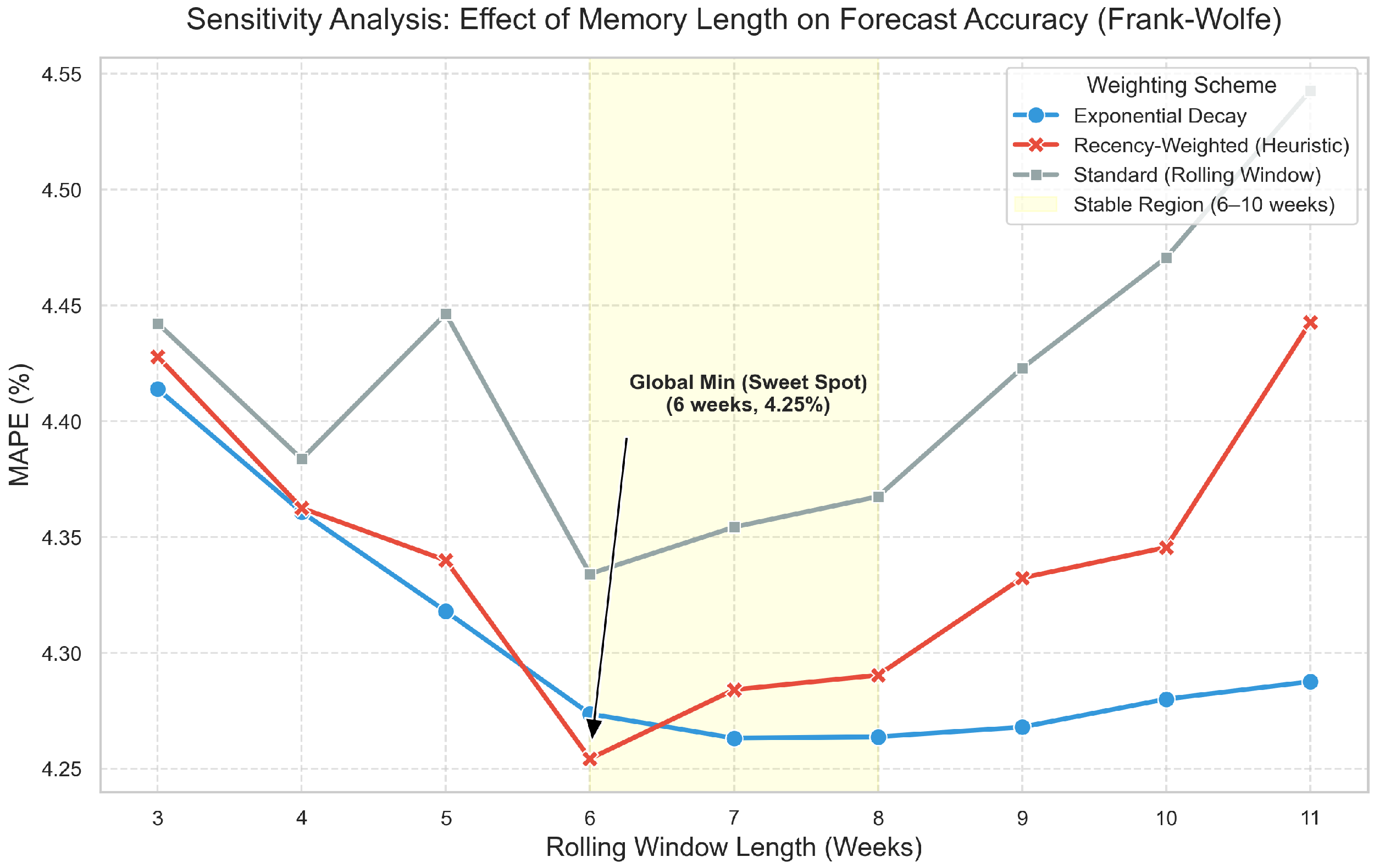
. To determine the optimal length of the historical window H, we evaluate various sizes ranging from 3 to 11 weeks. The specific window size that achieves the lowest error on the validation set is subsequently selected for the final evaluation on the test set. This empirical approach ensures a proper balance between gathering sufficient statistical history and maintaining adaptability to new weather regimes.

4. Results

The proposed methodology was evaluated on an independent test set spanning a full year to ensure reliable results across different seasons.

4.1. Base Model Performance

The performance of individual models varied significantly as shown in

Table 3. Performance of individual base learners (sorted by MAPE).

Model	MAE (MWh)	RMSE (MWh)	MAPE (%)
N-HiTS	10,253	13,893	5.31
Temporal Fusion Transformer (TFT)	10,050	13,321	5.43
CatBoost	13,798	18,447	7.37
LightGBM	13,437	17,888	7.35
Support Vector Regression (SVR)	14,726	20,483	7.74
XGBoost	14,560	19,338	7.76
ExtraTrees	15,117	19,453	8.32
ARX (Robust)	14,946	18,659	9.17
Bayesian Ridge	14,852	18,451	9.18
ElasticNet	17,071	20,510	10.67
NeuralProphet	17,963	22,245	11.74
KNN	21,115	26,519	12.37
LSTM	21,293	26,591	12.91
SARIMAX	18,840	25,071	13.05
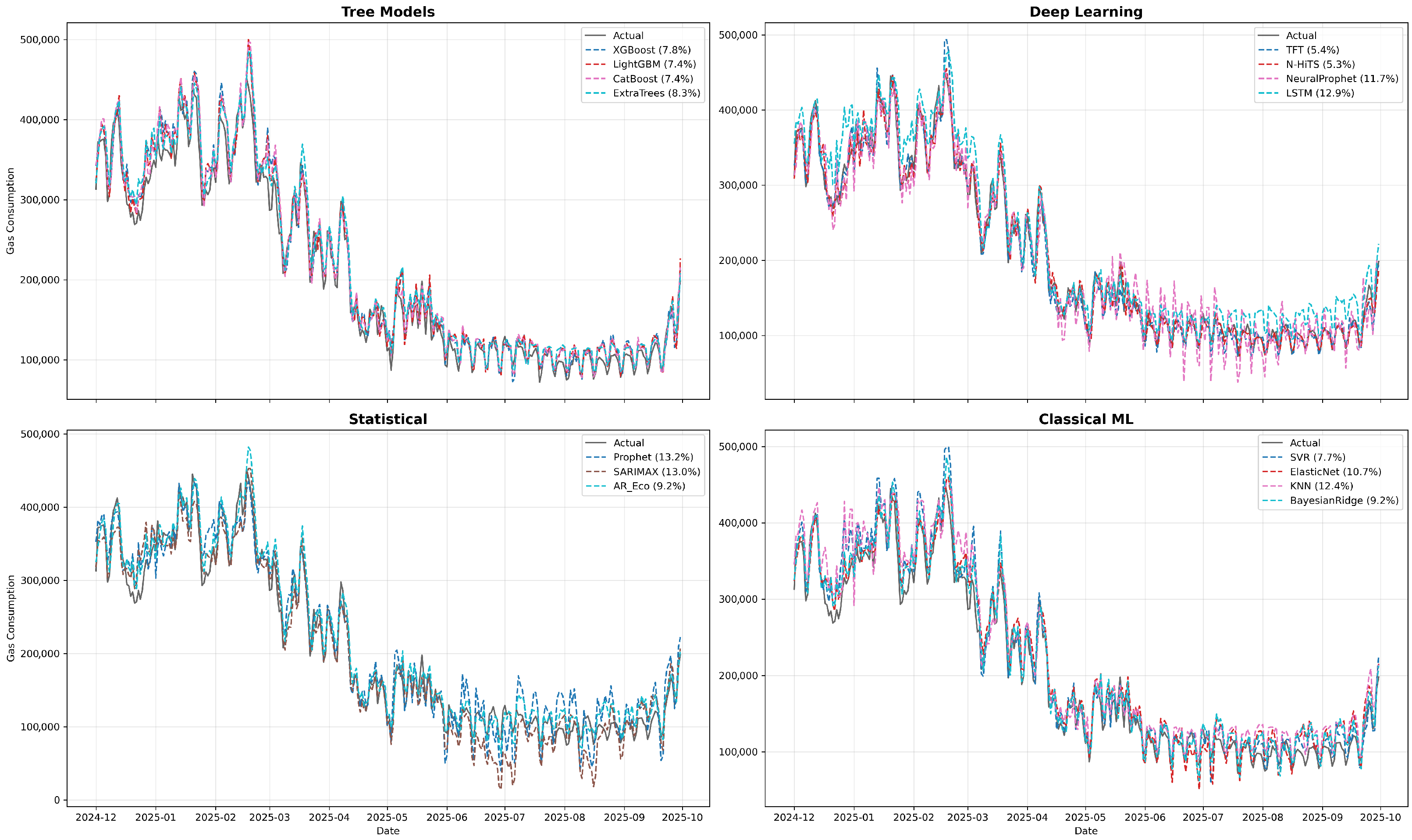
Prophet	19,161	24,113	13.15

. The N-HiTS model emerged as the best single predictor with a Mean Absolute Percentage Error (MAPE) of 5.31%. It was closely followed by the Temporal Fusion Transformer (TFT) at 5.43%. Tree-based models including CatBoost, XGBoost, and LightGBM yielded MAPEs ranging from 7.35% to 7.76%.

A visual comparison of the predictions from base model groups with actual consumption is shown in Figure 1.

4.2. Ensemble Optimization Results

The application of dynamic weighting strategies yielded measurable improvements.

Table 4. Comparison of optimal ensemble strategies (six week window).

Strategy	MAE	RMSE	MAPE (%)
Frank–Wolfe (6 weeks, Weighted)	8235	11,375	4.25
Ensemble Selection (6 weeks, Weighted)	8279	11,447	4.26
Ensemble Selection (6 weeks, Exponential)	8202	11,260	4.26
Frank–Wolfe (6 weeks, Exponential)	8221	11,345	4.27
NNLS (6 weeks, Weighted)	9000	12,379	4.66
Benchmarks:
Best Single Model (N-HiTS)	10,253	13,893	5.31
Contextual Bandit (Online)	10,050	13,321	5.43
Simple Ensemble Average	11,723	14,897	6.74

summarizes the performance of different optimization strategies using a history window of six weeks. This window length proved to be optimal in our extended analysis.

The optimized ensemble achieved a MAPE of 4.25%. This result reduces the error by more than one percentage point relative to the best single model and by 2.5 percentage points compared to static averaging. Our extended analysis identified that a lookback window of six weeks provides an ideal balance for these calculations. As visualized in Figure 2, model stability increases up to six weeks before data drift begins to negatively affect the results. To validate the temporal weighting strategy, we compared our proposed recency-weighted heuristic against a standard exponential decay. The weighted approach performed slightly better, achieving 4.25% compared to the 4.27% error rate of the exponential decay within the Frank–Wolfe framework.

When evaluated against alternative optimization strategies, the Frank–Wolfe algorithm consistently outperformed the standard non-negative least squares approach. This advantage can be attributed to the iterative nature of the Frank–Wolfe algorithm, which acts as an effective regularization technique against overfitting. Finally, we recorded the execution times to assess the computational complexity and operational feasibility of the framework. Training the deep learning base learners required approximately two to four hours on the standard workstation. In contrast, the Frank–Wolfe ensemble optimization across the entire test set took less than five seconds. This indicates that once the base predictions are available, the dynamic weight adaptation introduces negligible overhead.

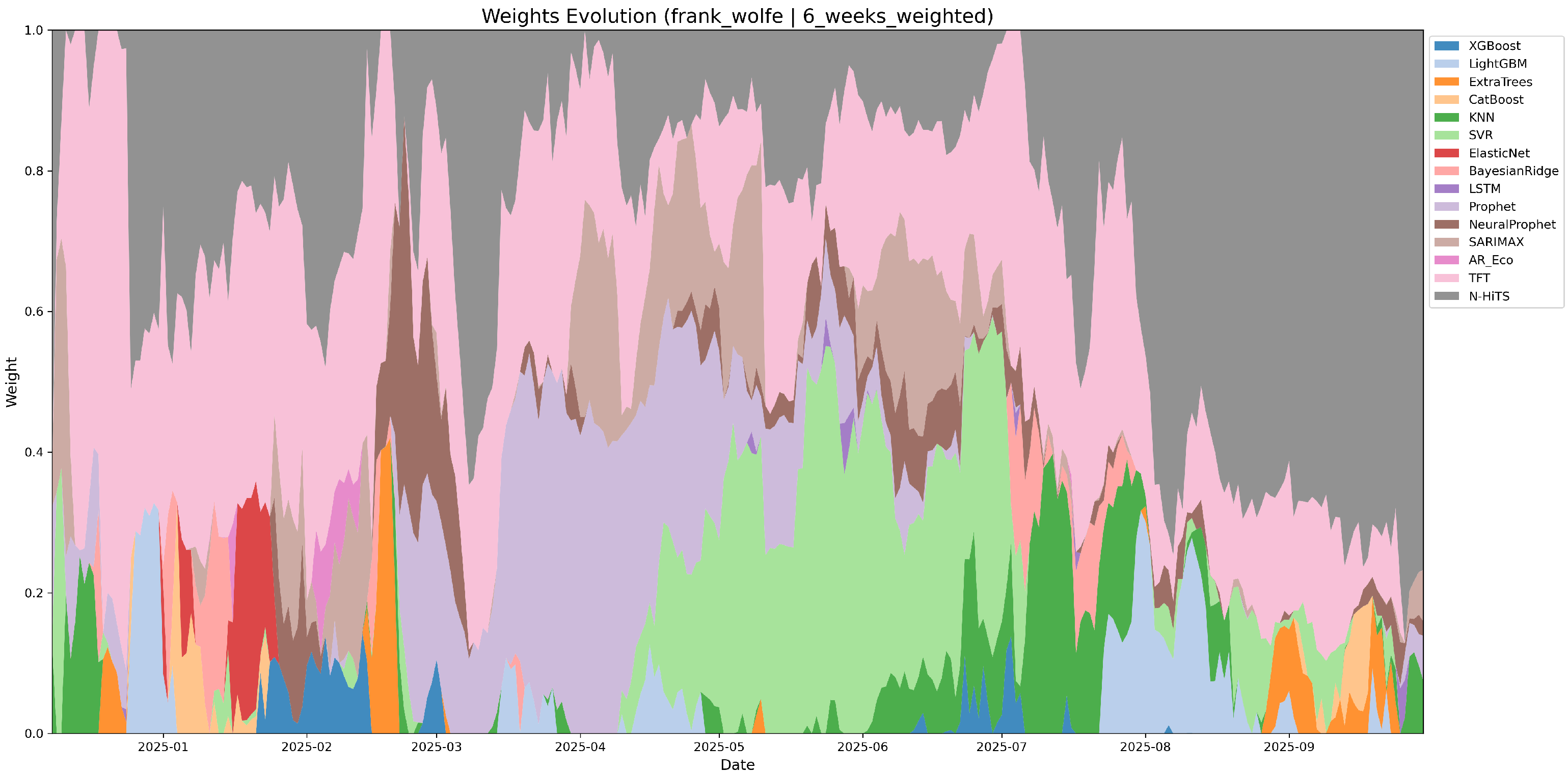
Figure 3 illustrates the evolution of weights for the winning strategy. The system dynamically reallocates weights to mitigate the failure of any single predictor.

To complement the visualization and address the interpretability of the dynamic weight allocation,

Table 5. Average weight allocation ($\overline{w}$) assigned by the Frank–Wolfe optimizer (recency-weighted strategy). Models with negligible weights (<1%) are aggregated.

Model Family	Base Learner	Avg.Weight (%)
Deep Learning	N-HiTS	29.3%
	TFT	27.5%
	NeuralProphet	3.6%
Classical ML	SVR	10.0%
	KNN	4.7%
	BayesianRidge	1.5%
	ElasticNet	1.0%
Statistical	Prophet	9.2%
	SARIMAX	5.7%
Tree-Based	LightGBM	3.1%
	XGBoost	1.4%
	ExtraTrees	1.3%
	CatBoost	1.2%
Other	Others (aggregated)	0.6%

presents the average weight contribution of the top performing base learners over the test period. The Frank–Wolfe algorithm inherently promotes sparsity. Out of 15 available models, it relies heavily on a smaller subset and effectively filters out noise from weaker predictors.

4.3. Statistical Significance Testing

To determine whether the observed improvements in forecast accuracy are statistically significant or artifacts of stochastic variation, we conducted nonparametric testing. The purpose of making these different comparisons is to rigorously evaluate whether the continuous convex optimization method statistically differentiates itself from both discrete heuristics and individual base learners. To ensure an equitable evaluation, all implemented ensemble solution methods and the best single models were compared across all tests over the entire test set. A significance level of 5% ($\alpha =0.05$) was used for all tests.

4.3.1. Diebold–Mariano Test

We employed the Diebold–Mariano test to compare the proposed Frank–Wolfe strategy with the second best alternative, which is Ensemble Selection. The null hypothesis states that both forecasting methods have equal predictive accuracy. The test statistic was calculated based on the Mean Absolute Error differential series in Equation (3):

$$d_t=|e_{1,t}|-|e_{2,t}|$$

(3)

where $e_{1,t}$ and $e_{2,t}$ denote the forecast errors of the primary model and the benchmark model at time t, respectively. The results yielded a test statistic of $-1.11$ with a p-value of $0.2669$. Consequently, we fail to reject the null hypothesis at the established 5% significance level. This confirms the observation that the raw accuracy difference between the best ensemble strategies is marginal. While the proposed method does not statistically outperform Ensemble Selection in raw accuracy, its practical preference is justified by computational stability and sparsity properties rather than error reduction.

4.3.2. Friedman Test and Pairwise Significance

To assess the hierarchy of methods, we followed the methodology recommended by [31] for comparing algorithms over multiple datasets. We employed the nonparametric Friedman test to detect global differences, followed by a Nemenyi post hoc analysis for pairwise comparisons. Furthermore, to evaluate the specific significance of the improvement relative to the best baseline, we used the Diebold–Mariano test [32].

The Friedman test rejected the null hypothesis of equal performance with a p-value below $0.001$.

Table 6. Pairwise statistical significance (Nemenyi Test, $\alpha =0.05$).

Comparison Pair (A vs. B)	p-Value	Significant	Winner
Frank–Wolfe vs. Ensemble Selection	0.998	No	Draw
Frank–Wolfe vs. N-HiTS (Best Single)	<0.01	Yes	Frank–Wolfe
Frank–Wolfe vs. XGBoost	<0.001	Yes	Frank–Wolfe
Frank–Wolfe vs. Simple Averaging	<0.001	Yes	Frank–Wolfe
N-HiTS vs. XGBoost	<0.05	Yes	N-HiTS

synthesizes the pairwise statistical significance between the proposed Frank–Wolfe ensemble and key benchmarks.

The results confirm that while the difference between the two sophisticated ensemble methods (FW and ES) is not statistically significant, both form a statistically superior cluster compared to individual state-of-the-art models and simple averaging.

4.3.3. Ablation Study

To isolate the contribution of the proposed optimization framework, we performed an ablation study comparing the complete Frank–Wolfe ensemble against simplified baselines.

Table 7. Ablation study quantifying the impact of ensemble components on forecast accuracy (MAPE).

Component Level	Method Description	MAPE (%)	Rel. Improvement
1. Baseline	Best Single Model (N-HiTS)	5.31%	−
2. Naïve Comb.	Simple Ensemble Average (Mean)	6.74%	−26.9%
3. Standard Opt.	NNLS (Rolling Window)	4.60%	+13.4%
4. Dynamic Opt.	Frank–Wolfe (Rolling Window)	4.33%	+18.5%
5. Proposed	Frank–Wolfe + Temporal Weighting	4.25%	+20.0%

demonstrates the incremental gain from each component of the proposed methodology.

The results indicate that simple averaging actually deteriorates performance due to the inclusion of weaker learners. The introduction of convex optimization restores performance. However, the most notable leap in accuracy is achieved by making the optimization dynamic and context aware.

5. Discussion

The empirical results support the premise that applying operations research methods to prediction weighting provides a transparent and controllable mechanism for improving forecast accuracy. The evaluated six week weighted window serves as a highly effective heuristic for the Czech gas market.

Although the difference in accuracy between the Frank–Wolfe approach and Ensemble Selection is statistically negligible, the continuous optimization method offers distinct advantages for production environments. A granular inspection of the weight evolution reveals a critical operational difference rooted in the mathematical nature of the algorithms. Ensemble Selection is a discrete greedy algorithm that selects models from a finite set. This leads to abrupt weight changes where the algorithm suddenly shifts confidence from one model to another based on marginal short term gains. In contrast, the Frank–Wolfe algorithm operates in a continuous space on the unit simplex. It produces smooth and gradual weight reallocations. This behavior avoids the sudden jumps typical of greedy heuristics. For a market operator, this smoothness minimizes operational risk and transaction costs associated with abrupt daily shifts in trading strategies. This practical benefit justifies the preference for the convex optimization approach despite the parity in raw accuracy.

This observation aligns with the forecast combination puzzle discussed by [33], where sophisticated weighting schemes often yield only marginal gains over simple averages due to estimation noise. Our results demonstrate that the primary value of convex optimization lies not merely in error reduction but in the stability and sparsity of the solution. Furthermore, unlike opaque automated machine learning solutions, the proposed framework maintains high interpretability. The weight vector directly represents the confidence in each underlying model. It effectively treats the forecast as an investment portfolio.

A critical consideration for operational deployment is computational complexity, addressing the limitations of current solution methods. Training deep learning architectures like N-HiTS or Temporal Fusion Transformers requires significant computational resources. The training phase for these neural networks has a high time complexity and typically requires hardware acceleration for frequent recalibration. In contrast, the proposed Frank–Wolfe weight optimization acts as a lightweight meta learner. The Linear Minimization Oracle at each iteration of the Frank–Wolfe algorithm has a time complexity of $\mathcal{O}\left(N\right)$, where N is the number of base learners. For a historical window of length H and K iterations, the total complexity of the weight update step is strictly bounded by $\mathcal{O}(K·N·H)$. Because N and H are very small in our daily forecasting setup, the optimization converges in a matter of seconds on a standard central processing unit. This allows market operators to update the ensemble weights daily with virtually no additional computational cost, successfully decoupling the heavy base model training phase from the rapid daily adaptation phase.

Finally, it is worth noting the performance of statistical baselines. The Prophet model was included primarily as a representative benchmark for generalized additive models. The observed performance difference relative to deep learning models suggests that the default additive assumptions require extensive manual feature engineering to fully capture the changing variance in gas demand. Conversely, the gradient boosting and deep learning approaches demonstrated a greater capacity to autonomously extract these nonlinear dependencies from the same meteorological inputs.

6. Conclusions

This study reformulated the daily natural gas consumption forecasting task from a model selection problem to a constrained convex optimization problem on the unit simplex. By applying the Frank–Wolfe algorithm, we established a mathematical framework that guarantees convergence to a global optimum for convex loss functions. This approach addresses the lack of theoretical grounding found in many standard heuristic ensembles.

6.1. Synthesis of Empirical and Theoretical Findings

Our results demonstrate that dynamic convex optimization offers measurable improvements over both individual base models and static ensemble techniques. The proposed framework achieved a Mean Absolute Percentage Error of 4.25%, which represents a statistically significant improvement over the best single deep learning model at 5.31% and the simple ensemble average at 6.74%.

The ablation study quantified the sources of this improvement. Transitioning from static weights to time-varying weights yielded a relative accuracy gain of approximately 9%, indicating that adapting to concept drift is as important as initial model selection. Furthermore, we showed that the optimal lookback window of six weeks reflects the quasi stationarity period of seasonal consumption patterns. Similarly, the recency weighted heuristic aligns with the physical inertia of synoptic weather systems in Central Europe, acting as an effective Bayesian prior for the optimization process.

While the Diebold–Mariano test indicated parity in raw accuracy between the Frank–Wolfe optimization and the greedy Ensemble Selection method, the convex approach is preferred for operational deployment. Unlike greedy algorithms that select from discrete sets, the Frank–Wolfe algorithm operates in continuous space. It produces sparse and stable weight vectors that minimize transaction costs in daily decision making.

6.2. Limitations and Future Research Directions

The validity of these findings is bound by the specific regulatory and climatic context of the Czech Republic and the use of retrospective reanalysis data. Operational implementation would introduce additional uncertainty caused by errors in numerical weather predictions. In addition, the computational cost of retraining deep learning base learners remains a limitation for high frequency updates.

Future research will extend this framework in four primary directions:

• Data Availability: The study is validated on a test set spanning a single gas year. While this captures a complete seasonal cycle including transitions between heating and non-heating periods, testing on multiple years is necessary to evaluate the methodology against long term climatic anomalies such as extremely mild winters.
• Online Learning: Replacing the batch based rolling window with fully online algorithms, such as weighted linear bandits, could reduce computational complexity per step and improve real time adaptation.
• Probabilistic Forecasting: Generalizing the loss function from a point estimate metric to quantile regression will allow the generation of conformal prediction intervals. These intervals are essential for risk aware bidding strategies.
• Multi Energy Coupling: Incorporating renewable energy generation as exogenous variables will help capture the increasing cross commodity correlations in modern energy grids.

References

- OTE, a.s. Metodika Teplotního Přepočtu TDD pro rok 2023. 2025. Available online: https://www.ote-cr.cz/ (accessed on 15 November 2025).
- Özmen, A.; Yılmaz, Y.; Weber, G.-W. Natural gas consumption forecast with MARS and CMARS models for residential users. Energy Econ. 2018, 70, 357–381. [Google Scholar] [CrossRef] [Scilit]
- Potočnik, P.; Soldo, B.; Šimunović, G.; Šarić, T.; Jeromen, A.; Govekar, E. Comparison of static and adaptive models for short-term residential natural gas forecasting in Croatia. Appl. Energy 2014, 129, 94–103. [Google Scholar] [CrossRef] [Scilit]
- Chen, T.; Guestrin, C. XGBoost: A Scalable Tree Boosting System. In Proceedings of the 22nd ACM SIGKDD International Conference on Knowledge Discovery and Data Mining; ACM: New York, NY, USA, 2016; pp. 785–794. [Google Scholar] [CrossRef] [Scilit]
- Ke, G.; Meng, Q.; Finley, T.; Wang, T.; Chen, W.; Ma, W.; Ye, Q.; Liu, T.-Y. LightGBM: A Highly Efficient Gradient Boosting Decision Tree. Adv. Neural Inf. Process. Syst. 2017, 30, 3149–3157. Available online: https://dl.acm.org/doi/10.5555/3294996.3295074 (accessed on 15 November 2025).
- Wang, J.Q.; Du, Y.; Wang, J. LSTM based long-term energy consumption prediction with periodicity. Energy 2020, 197, 117197. [Google Scholar] [CrossRef] [Scilit]
- Oliveira, M.; Torgo, L. Ensembles for time series forecasting. In Asian Conference on Machine Learning; PMLR: Cambridge, MA, USA, 2015; pp. 360–370. [Google Scholar]
- Boyd, S.; Vandenberghe, L. Convex Optimization; Cambridge University Press: Cambridge, UK, 2004. [Google Scholar] [CrossRef] [Scilit]
- Jaggi, M. Revisiting Frank-Wolfe: Projection-Free Sparse Convex Optimization. In Proceedings of the 30th International Conference on Machine Learning; ACM: New York, NY, USA, 2013; pp. 427–435. Available online: https://dl.acm.org/doi/10.5555/3042817.3042867 (accessed on 15 November 2025).
- Caruana, R.; Niculescu-Mizil, A.; Crew, G.; Ksikes, A. Ensemble selection from libraries of models. In Proceedings of the 21st International Conference on Machine Learning; ACM: New York, NY, USA, 2004; p. 18. [Google Scholar]
- Taylor, S.J.; Letham, B. Forecasting at Scale. Am. Stat. 2018, 72, 37–45. [Google Scholar] [CrossRef] [Scilit]
- Smajla, I.; Vulin, D.; Sedlar, D.K. Short-term forecasting of natural gas consumption by determining the statistical distribution of consumption data. Energy Rep. 2023, 10, 2352–2360. [Google Scholar] [CrossRef] [Scilit]
- Dudek, G. A Comprehensive Study of Random Forest for Short-Term Load Forecasting. Energies 2021, 15, 7547. [Google Scholar] [CrossRef] [Scilit]
- Svoboda, R.; Kotik, V.; Platos, J. Short-term natural gas consumption forecasting from long-term data collection. Energy 2021, 218, 119430. [Google Scholar] [CrossRef] [Scilit]
- Lim, B.; Arik, S.O.; Loeff, N.; Pfister, T. Temporal Fusion Transformers for Interpretable Multi-horizon Time Series Forecasting. Int. J. Forecast. 2021, 37, 1748–1764. [Google Scholar] [CrossRef] [Scilit]
- Challu, C.; Olivares, K.G.; Oreshkin, B.N.; Ramirez, F.G.; Canseco, M.M.; Dubrawski, A. N-HiTS: Neural Hierarchical Interpolation for Time Series Forecasting. In Proceedings of the AAAI Conference on Artificial Intelligence; Association for the Advancement of Artificial Intelligence: Washington, DC, USA, 2023; Volume 37, pp. 6989–6997. [Google Scholar] [CrossRef] [Scilit]
- Zhao, M.; Guo, G.; Fan, L.; Han, L.; Yu, Q.; Wang, Z. Short-term natural gas load forecasting based on EL-VMD-Transformer-ResLSTM. Sci. Rep. 2024, 14, 20343. [Google Scholar] [CrossRef] [Scilit]
- Panapakidis, I.P.; Dagoumas, A.S. Day-ahead natural gas demand forecasting based on the combination of wavelet transform and ANFIS/genetic algorithm/neural network model. Energy 2017, 118, 231–245. [Google Scholar] [CrossRef] [Scilit]
- Wu, H.; Levinson, D. The Ensemble Approach to Forecasting: A Review and Synthesis. Transp. Res. Part C Emerg. Technol. 2021, 132, 103357. [Google Scholar] [CrossRef] [Scilit]
- Li, F.; Sun, M. EMLP: Short-term gas load forecasting based on ensemble multilayer perceptron with adaptive weight correction. Math. Biosci. Eng. 2021, 18, 1590–1608. [Google Scholar] [CrossRef] [Scilit] [PubMed]
- Box, G.E.P.; Jenkins, G.M.; Reinsel, G.C.; Ljung, G.M. Time Series Analysis: Forecasting and Control, 5th ed.; John Wiley & Sons: Hoboken, NJ, USA, 2015. [Google Scholar] [CrossRef] [Scilit]
- Sharma, V.; Cali, Ü.; Sardana, B.; Kuzlu, M.; Banga, D.; Pipattanasomporn, M. Data-driven short-term natural gas demand forecasting with machine learning techniques. J. Pet. Sci. Eng. 2021, 206, 108979. [Google Scholar] [CrossRef] [Scilit]
- Marziali, A.; Fabbiani, E.; De Nicolao, G. Ensembling methods for countrywide short-term forecasting of gas demand. Int. J. Oil, Gas Coal Technol. 2021, 26, 184–201. [Google Scholar] [CrossRef] [Scilit]
- Liu, Y.; Jiang, Z.; Leng, W. A Study on Predicting Natural Gas Prices Utilizing Ensemble Model. Sustainability 2025, 17, 8514. [Google Scholar] [CrossRef] [Scilit]
- Prokhorenkova, L.; Gusev, G.; Vorobev, A.; Dorogush, A.V.; Gulin, A. CatBoost: Unbiased Boosting with Categorical Features. Adv. Neural Inf. Process. Syst. 2018, 31, 6639–6649. [Google Scholar] [CrossRef] [Scilit]
- Frank, M.; Wolfe, P. An algorithm for quadratic programming. Nav. Res. Logist. Q. 1956, 3, 95–110. [Google Scholar] [CrossRef] [Scilit]
- De Myttenaere, A.; Golden, B.; Le Grand, B.; Rossi, F. Mean absolute percentage error for regression models. Neurocomputing 2016, 192, 38–48. [Google Scholar] [CrossRef] [Scilit]
- Zippenfenig, P. Zenodo, Version 1.4.0; Open-Meteo.com Weather API [Computer Software]. Zenodo; CERN: Geneva, Switzerland, 2023. [CrossRef]
- Pedregosa, F.; Varoquaux, G.; Gramfort, A.; Michel, V.; Thirion, B.; Grisel, O.; Blondel, M.; Prettenhofer, P.; Weiss, R.; Dubourg, V.; et al. Scikit-learn: Machine Learning in Python. J. Mach. Learn. Res. 2011, 12, 2825–2830. [Google Scholar] [CrossRef] [Scilit]
- Paszke, A.; Gross, S.; Massa, F.; Lerer, A.; Bradbury, J.; Chanan, G.; Killeen, T.; Lin, Z.; Gimelshein, N.; Antiga, L.; et al. PyTorch: An Imperative Style, High-Performance Deep Learning Library. Adv. Neural Inf. Process. Syst. 2019, 32, 8026–8037. [Google Scholar] [CrossRef] [Scilit]
- Demšar, J. Statistical comparisons of classifiers over multiple data sets. J. Mach. Learn. Res. 2006, 7, 1–30. Available online: https://dl.acm.org/doi/10.5555/1248547.1248548 (accessed on 15 November 2025).
- Diebold, F.X.; Mariano, R.S. Comparing predictive accuracy. J. Bus. Econ. Stat. 2002, 20, 134–144. [Google Scholar] [CrossRef] [Scilit]
- Elliott, G.; Liao, J. Combining Forecasts-On Why Averaging beats Optimal Linear Weights; University of California: San Diego, CA, USA, 2025. [Google Scholar]