Diverse Jacobi Elliptic Function Solutions and Dynamical Behaviors for a High-Order KdV Type Wave Equation via Extended F-Expansion Method

Abstract

This paper focuses on a high-order Korteweg–de Vries wave equation. The extended F-expansion method, a modified form of Kudryashov’s auxiliary equation approach, is employed to construct Jacobi elliptic function solutions for this equation. Three distinct families of solutions are obtained, including solitary waves, breathers, dark/bright solitons, bright–dark interaction solitons, and rogue-like solutions. To better illustrate the complex nonlinear dynamics of the high-order Korteweg–de Vries wave equation, representative solutions are selected, and their moduli are visualized using Maple software through three-dimensional, two-dimensional, and contour plots.

1. Introduction

Nowadays, the task of finding exact solutions to nonlinear partial differential equations has attracted increasing attention. These equations serve as fundamental mathematical tools for describing complex nonlinear physical phenomena, with applications spanning diverse fields, including engineering, applied mathematics, chemistry, biology, mechanics, and physics. For this reason, studying the explicit solutions of nonlinear evolution equations (NLEEs) holds a key position in mathematical physics and in the development of many physical models.

As a representative example, a generalized Korteweg–de Vries type equation has the following form:

$$\begin{array}{cc}\hfill {\varphi }_t& +{\varphi }_x+\alpha \varphi {\varphi }_x+\beta {\varphi }_{xxx}+{\rho }_1{\alpha }^2{\varphi }^2{\varphi }_x+\alpha \beta \left({\rho }_2\varphi {\varphi }_{xxx}+{\rho }_3{\varphi }_x{\varphi }_{xx}\right)\hfill \\ \hfill & +{\rho }_4{\alpha }^3{\varphi }^3{\varphi }_x+{\alpha }^2\beta \left({\rho }_5{\varphi }^2{\varphi }_{xxx}+{\rho }_6\varphi {\varphi }_x{\varphi }_{xx}+{\rho }_7{\varphi }_x^3\right)=0,\hfill \end{array}$$

(1)

where $\alpha ={\displaystyle \frac{3A}{2}}$, $\beta ={\displaystyle \frac{B}{6}}$, ${\rho }_1=-{\displaystyle \frac{1}{6}}$, ${\rho }_2={\displaystyle \frac{5}{3}}$, ${\rho }_3={\displaystyle \frac{23}{6}}$, ${\rho }_4={\displaystyle \frac{1}{8}}$, ${\rho }_5={\displaystyle \frac{7}{18}}$, ${\rho }_6={\displaystyle \frac{79}{36}}$, ${\rho }_7={\displaystyle \frac{45}{36}}$. This equation was derived by Fokas [1] in 1995 based on physical and asymptotic analyses. By incorporating higher-order nonlinear terms and dispersive correction terms, it can more accurately describe a rich variety of nonlinear wave phenomena. These include the propagation of high-amplitude water waves in deep water or coastal regions, internal gravity waves in stratified fluids within fluid dynamics, the formation and interaction of solitons in intense ion-acoustic waves in plasma physics, and the evolution of ultra-short optical pulses in fibers for nonlinear optics. Additionally, by treating the ${\rho }_i$$(i=1,2,\dots ,7)$ as free unknowns and neglecting all higher-order correction terms, the classical KdV equation can be obtained:

$$\begin{array}{c}\hfill {\varphi }_t+{\varphi }_x+\alpha \varphi {\varphi }_x+\beta {\varphi }_{xxx}=0.\end{array}$$

(2)

when $\alpha =6$ and $\beta =1$, this equation reduces to the standard form of the KdV equation [2], which was first derived by D. J. Korteweg and G. de Vries in 1895 to model the propagation of long water waves in shallow rectangular channels:

$$\begin{array}{c}\hfill {\varphi }_t+{\varphi }_x+6\varphi {\varphi }_x+{\varphi }_{xxx}=0.\end{array}$$

(3)

In this paper, based on Fokas’s assumption that $O\left(\beta \right)<O\left(\alpha \right)$, a high-order Korteweg–de Vries equation (HOKdV) is considered. This equation is obtained by neglecting two high-order infinitesimal terms of $O\left({\alpha }^3,{\alpha }^2\beta \right)$ to derive its explicit solutions:

$$\begin{array}{c}\hfill {\varphi }_t+{\varphi }_x+\alpha \varphi {\varphi }_x+\beta {\varphi }_{xxx}+{\rho }_1{\alpha }^2{\varphi }^2{\varphi }_x+\alpha \beta \left({\rho }_2\varphi {\varphi }_{xxx}+{\rho }_3{\varphi }_x{\varphi }_{xx}\right)=0,\end{array}$$

(4)

where ${\rho }_i$$(i=1,2,3)$ are regarded as free parameters. The equation was initially derived in [3] via the bi-Hamiltonian system approach.

Over the past few decades, a wide range of approaches have been successively proposed for solving the KdV equation, each with unique advantages and inherent limitations. The inverse scattering transform [4], renowned for its mathematical rigor, offers a powerful framework for constructing multi-soliton solutions, yet its applicability is restricted to completely integrable systems due to its inherent complexity. The Hirota method [5] reformulates the KdV equation via a bilinear transformation, which simplifies the algebraic construction of multi-soliton solutions. Despite its elegance, this approach faces constraints when dealing with complex boundary conditions or nonlocal formulations. The homogeneous balance method [6] determines the structure of solutions by balancing the highest-order linear and nonlinear terms. While efficient for constant-coefficient KdV-type equations, its reliance on empirically chosen balancing parameters restricts its broader use. The Jacobi elliptic function method [7] broadens the scope of solvable KdV equation cases by introducing periodic and hyperbolic function assumptions. It is effective for deriving periodic and solitary wave solutions, but the associated computations are intensive, and only specific solution forms can be obtained. The tanh-function method [8] has a simple form and is easy to implement, efficiently constructing solitary wave solutions for the KdV equation. However, it is limited to solutions expressed in terms of hyperbolic functions and struggles with variable-coefficient or nonlocal equations. The exp-function method [9] is straightforward and applicable to various nonlinear equations, but it often yields formal solutions with limited physical interpretation. The Lax pair method [10] can rigorously verify the complete integrability of the KdV equation and construct its multi-soliton solutions. Nevertheless, it lacks universality and is technically challenging to apply to non-integrable or complex nonlinear systems. The F-expansion method [11] is universal and straightforward, systematically yielding periodic wave solutions and soliton solutions for the KdV equation. However, it depends on known solutions of the auxiliary equation, and its application scope is constrained by the form of the nonlinear equation.

In this paper, an improved variant of Kudryashov’s auxiliary equation approach [12,13,14,15] is adopted as the primary tool to conduct an in-depth investigation of the HOKdV Equation (4). First formulated in the late 1980s, this mathematical technique experienced a revival via Kudryashov’s reintroduction in 2011. Separately, the extended F-expansion method, an analytical scheme put forward by Engui Fan [16], takes Jacobi elliptic functions as its fundamental theoretical basis [17,18,19]. This particular approach exhibits notable efficacy in deriving a wide range of elliptic function solutions for NLEEs. Compared with early methods for solving the KdV equation, the extended F-expansion method introduces solution forms with combined positive and negative power terms and a more general elliptic auxiliary equation, enabling it to obtain various explicit solutions and apply to more general nonlinear equations. To gain a comprehensive and systematic understanding of the targeted equation system, it is necessary to derive a diverse set of explicit solutions for the HOKdV Equation (4), followed by the use of graphical visualization techniques to characterize the intricate dynamical properties exhibited by these solutions within the complex plane.

The remainder of this paper is structured as follows: In Section 2, we provide a concise overview of the F-expansion method, which serves as a key analytical tool for addressing the HOKdV Equation (4). In Section 3, we construct three distinct sets of solutions and derive the associated Jacobi elliptic solutions, dark/bright solitons, breathers, and solitary waves. In Section 4, we select several representative and noteworthy solutions, generating three-dimensional, two-dimensional, and contour plots to investigate their intricate dynamical behavior. Finally, Section 5 presents the concluding remarks of this work.

2. Extended F-Expansion Technique

In this section, a concise overview is presented of the extended F-expansion technique, a modified version of Kudryashov’s auxiliary equation method. For a nonlinear partial differential equation:

$$\begin{array}{c}\hfill F\left(u,u_t,u_{x_1},u_{x_1{x}_1},u_{x_1{x}_2},u_{t{x}_1},\dots \right)=0,\end{array}$$

(5)

the following traveling wave transformation is considered:

$$\begin{array}{c}\hfill u\left(x_1,x_2,\dots ,t\right)=\varphi \left(s\right),s={\alpha }_1{x}_1+{\alpha }_2{x}_2+\dots -\beta t,\end{array}$$

(6)

where ${\alpha }_j,j=1,2,\dots$ and $\beta$ are undetermined constants. Substituting transformation (6) into Equation (5) reduces the nonlinear partial differential equation to an ordinary differential equation:

$$\begin{array}{c}\hfill G\left(\varphi ,{\varphi }^{\prime },{\varphi }^{\prime \prime },{\varphi }^{\prime \prime \prime },\dots \right)=0.\end{array}$$

(7)

Once the undetermined coefficients in the transformation (6) are fixed, the solutions to Equation (7) can be obtained. Furthermore, the solution to Equation (7) can be assumed to take the form [20,21]:

$$\begin{array}{c}\hfill \varphi \left(s\right)=A_0+\sum _{i=1}^N\left[A_i{f}^i\left(s\right)+B_i{f}^{-i}\left(s\right)\right],\end{array}$$

(8)

where $A_0,A_i,B_i,i=1,2,\dots ,N$ are undetermined constants, and N is determined via the homogenous balance principle. More precisely, if the degree of $\varphi \left(s\right)$ is defined as $O\left(\varphi \right(s\left)\right)$, the homogeneous balance principle for Equation (7) can be expressed as follows [22,23]:

$$\begin{array}{c}\hfill N+q=O\left({\displaystyle \frac{{\mathrm{d}}^q\varphi }{\mathrm{d}{\eta }^q}}\right)=O\left({\varphi }^p{\left({\displaystyle \frac{{\mathrm{d}}^q\varphi }{\mathrm{d}{\eta }^q}}\right)}^m\right)=Np+m(N+p),\end{array}$$

(9)

where $q,p,m$ are integers.This implies that the nonlinear term and the highest-order derivative term must share the same degree. Additionally, $f\left(s\right)$ satisfies the differential equation given below [24,25]:

$$\begin{array}{c}\hfill {\left({\displaystyle \frac{\mathrm{d}f\left(s\right)}{\mathrm{d}\eta }}\right)}^2={\mu }_0+{\mu }_{1}f\left(s\right)+{\mu }_2{f}^2\left(s\right)+{\mu }_3{f}^3\left(s\right)+{\mu }_4{f}^4\left(s\right),\end{array}$$

(10)

where ${\mu }_i,i=1,2,\dots ,4$ are constants.

By applying Kudryashov’s auxiliary equation method [26,27], the general solution to Equation (10) can be expressed in terms of Jacobi elliptic function in the following form:

$$\begin{array}{c}\hfill f\left(s\right)={\displaystyle \frac{f_1\left(f_3-f_2\right)s{n}^2\left[\frac{1}{2}\left(s-s_0\right)\sqrt{{\mu }_0\left(f_1-f_3\right)\left(f_4-f_2\right)};S\right]+f_2\left(f_1-f_3\right)}{\left(f_3-f_2\right)s{n}^2\left[\frac{1}{2}\left(s-s_0\right)\sqrt{{\mu }_4\left(f_1-f_3\right)\left(f_4-f_2\right)};S\right]+\left(f_1-f_3\right)}},\end{array}$$

(11)

where S represents the modulus of the Jacobi elliptic function, satisfying the following equation:

$$\begin{array}{c}\hfill S^2={\displaystyle \frac{\left(f_1-f_4\right)\left(f_1-f_3\right)}{\left(f_4-f_2\right)\left(f_3-f_2\right)}}.\end{array}$$

(12)

Here, $f_i,i=1,2,\dots ,4$ are roots of the following algebraic equation:

$$\begin{array}{c}\hfill {\mu }_0+{\mu }_{1}f\left(s\right)+{\mu }_2{f}^2\left(s\right)+{\mu }_3{f}^3\left(s\right)+{\mu }_4{f}^4\left(s\right)=0.\end{array}$$

(13)

In Equation (11), Jacobi elliptic functions represent a class of doubly periodic meromorphic functions defined over the complex plane, which are generalizations of trigonometric and hyperbolic functions. The modulus parameter S is the core parameter that determines their properties. Furthermore, $sn$ denotes the Jacobi sine elliptic function, one of the three fundamental Jacobi elliptic functions, alongside $cn$ and $dn$. They are doubly periodic on the complex plane; however, when the independent variable takes real values, this double periodicity manifests as single-periodic oscillations along the spatial or temporal direction, corresponding to the periodic wave solutions of the nonlinear equation.

The extended F-expansion technique can be viewed as a modified version of Kudryashov’s auxiliary equation method. The key distinction between the two approaches is that the extended F-expansion method leverages Equation (8) and Equation (10) to determine the values of undetermined coefficients, namely ${\alpha }_j,\beta ,A_0,A_i,B_i,i=1,2,\dots ,N,j=1,2,\dots$, and then substitutes these into Equation (6) to derive explicit solutions for Equation (5).

Equation (10), also referred to as the general elliptic equation, admits several special cases. When ${\mu }_0\ne 0$, ${\mu }_1\ne 0$, ${\mu }_2\ne 0$, ${\mu }_3\ne 0$ and ${\mu }_4\ne 0$, there exist three parameters $h_1$, $h_2$ and $h_3$ such that [28]

$$\begin{array}{cc}\hfill {\left({\displaystyle \frac{\mathrm{d}f\left(s\right)}{\mathrm{d}\eta }}\right)}^2& ={\mu }_0+{\mu }_{1}f\left(s\right)+{\mu }_2{f}^2\left(s\right)+{\mu }_3{f}^3\left(s\right)+{\mu }_4{f}^4\left(s\right)\hfill \\ \hfill & ={\left(h_1+h_{2}f\left(s\right)+h_3{f}^2\left(s\right)\right)}^2.\hfill \end{array}$$

(14)

Equation (14) is also known as the generalized Riccati equation [29] and it holds if and only if the following relations are satisfied:

$$\begin{array}{c}\hfill {\mu }_0=h_1^2,{\mu }_1=2h_1{h}_2,{\mu }_3=2h_2{h}_3,{\mu }_4=h_3^2,\end{array}$$

(15)

and the following constraint should exist between $h_1$, $h_2$ and $h_3$ parameters:

$$\begin{array}{c}\hfill h_2^2=-2h_1{h}_3,h_1{h}_3<0.\end{array}$$

(16)

When ${\mu }_0={\mu }_1=0$, the general elliptic equation reduces to the following auxiliary ordinary differential equation [30]:

$$\begin{array}{c}\hfill {\left({\displaystyle \frac{\mathrm{d}f\left(s\right)}{\mathrm{d}\eta }}\right)}^2={\mu }_2{f}^2\left(s\right)+{\mu }_3{f}^3\left(s\right)+{\mu }_4{f}^4\left(s\right).\end{array}$$

(17)

When ${\mu }_2={\mu }_4=0$, the general elliptic equation simplifies to

$$\begin{array}{c}\hfill {\left({\displaystyle \frac{\mathrm{d}f\left(s\right)}{\mathrm{d}\eta }}\right)}^2={\mu }_0+{\mu }_{1}f\left(s\right)+{\mu }_3{f}^3\left(s\right).\end{array}$$

(18)

When ${\mu }_1={\mu }_3=0$, the general elliptic equation simplifies to the elliptic equation:

$$\begin{array}{c}\hfill {\left({\displaystyle \frac{\mathrm{d}f\left(s\right)}{\mathrm{d}\eta }}\right)}^2={\mu }_0+{\mu }_2{f}^2\left(s\right)+{\mu }_4{f}^4\left(s\right).\end{array}$$

(19)

In this scenario, Equation (19) can yield multiple solutions for $f\left(s\right)$, depending on the specific values assigned to ${\mu }_0$, ${\mu }_2$ and ${\mu }_4$ as detailed in

Table 1. Jacobi elliptic solutions depending on the values of ${\mu }_0,{\mu }_2$ and ${\mu }_4$.

	${\mathsf{\mu }}_0$	${\mathsf{\mu }}_2$	${\mathsf{\mu }}_4$	f
1	1	$-\left(1+m^2\right)$	$m^2$	$\mathrm{sn}$
2	$1-m^2$	$2m^2-1$	$-m^2$	$\mathrm{cn}$
3	$m^2-1$	$2-m^2$	$-1$	$\mathrm{dn}$
4	$m^2$	$-\left(1+m^2\right)$	1	$\mathrm{ns}$
5	$-m^2$	$2m^2-1$	$1-m^2$	$\mathrm{nc}$
6	$-1$	$2-m^2$	$m^2-1$	$\mathrm{nd}$
7	1	$2-m^2$	$1-m^2$	$\mathrm{sc}$
8	1	$2m^2-1$	$-m^2\left(1-m^2\right)$	$\mathrm{sd}$
9	$m^2\left(1-m^2\right)$	$2m^2-1$	1	$-\mathrm{ds}$
10	$-{\displaystyle \frac{{\left(1-m^2\right)}^2}{4}}$	${\displaystyle \frac{m^2+1}{2}}$	$-{\displaystyle \frac{1}{4}}$	$m\mathrm{cn}\mp$ dn
11	${\displaystyle \frac{1}{4}}$	${\displaystyle \frac{-2m^2+1}{2}}$	${\displaystyle \frac{1}{4}}$	$\mathrm{nc}\mp \mathrm{cs}$
12	${\displaystyle \frac{1-m^2}{4}}$	${\displaystyle \frac{m^2+1}{2}}$	${\displaystyle \frac{1-m^2}{4}}$	$\mathrm{nc}\mp \mathrm{sc}$
13	${\displaystyle \frac{m^4}{4}}$	${\displaystyle \frac{m^2-2}{2}}$	${\displaystyle \frac{1}{4}}$	$\mathrm{ns}\mp \mathrm{ds}$
14	${\displaystyle \frac{m^4}{4}}$	${\displaystyle \frac{m^2-2}{2}}$	${\displaystyle \frac{m^2}{4}}$	$\mathrm{sn}\mp \mathrm{icn}$
15	${\displaystyle \frac{1}{4}}$	${\displaystyle \frac{m^2-2}{2}}$	${\displaystyle \frac{m^2}{4}}$	${\displaystyle \frac{\mathrm{sn}}{1\mp \mathrm{dn}}}$
16	${\displaystyle \frac{m^2-1}{4}}$	${\displaystyle \frac{m^2+1}{2}}$	${\displaystyle \frac{m^2-1}{4}}$	${\displaystyle \frac{\mathrm{dn}}{1\mp m\mathrm{sn}}}$
17	${\displaystyle \frac{1-m^2}{4}}$	${\displaystyle \frac{m^2+1}{2}}$	${\displaystyle \frac{1-m^2}{4}}$	${\displaystyle \frac{\mathrm{cn}}{1\mp \mathrm{sn}}}$
18	${\displaystyle \frac{1}{4}}$	${\displaystyle \frac{m^2+1}{2}}$	${\displaystyle \frac{{\left(1-m^2\right)}^2}{4}}$	${\displaystyle \frac{\mathrm{sn}}{\mathrm{dn}\mp \mathrm{cn}}}$

[31]. Here, m represents the modulus of Jacobi elliptic functions $(0<m<1)$. As m approaches 1 or 0, the Jacobi elliptic functions converge hyperbolic or trigonometric functions respectively [25,28], as illustrated in

Table 2. Jacobi elliptic functions approaching to hyperbolic or trigonometric functions.

	f	$\mathit{m}\to 1$	$\mathit{m}\to 0$
1	$\mathrm{sn}\omega$	$tanh\omega$	$sin\omega$
2	$\mathrm{cn}\omega$	$\mathrm{sech}\omega$	$cos\omega$
3	$\mathrm{dn}\omega$	$\mathrm{sech}\omega$	1
4	$\mathrm{sc}\omega$	$sinh\omega$	$tan\omega$
5	$\mathrm{sd}\omega$	$sinh\omega$	$sin\omega$
6	$\mathrm{cd}\omega$	1	$cos\omega$
7	$\mathrm{ns}\omega$	$coth\omega$	$csc\omega$
8	$\mathrm{nc}\omega$	$cosh\omega$	$sec\omega$
9	$\mathrm{nd}\omega$	$cosh\omega$	1
10	$\mathrm{cs}\omega$	$\mathrm{csch}\omega$	$cot\omega$
11	$\mathrm{ds}\omega$	$\mathrm{csch}\omega$	$csc\omega$
12	$\mathrm{dc}\omega$	1	$sec\omega$

.

Substituting Equation (8) into Equation (7) and employing Equation (10) along with its derivatives transforms the ordinary differential Equation (7) into a polynomial equation about $f^k\left(\eta \right),k=0,\pm 1,\pm 2,\dots$. By collecting different coefficients of $f^k\left(\eta \right)$ and equating them to zero, a system of linear equations is constructed for the undetermined coefficients ${\alpha }_j,\beta ,A_0,A_i,B_i,i=1,2,\dots ,N,j=1,2,\dots$. Substituting the values obtained from Table 1 and Table 2 into Equation (8) allows us to determine the structure of $\varphi \left(\eta \right)$, and thus the solutions of Equation (7) are ultimately derived.

Given the complexity of Equation (4), the extended F-expansion technique employed in this study is based on the elliptic Equation (19).

3. Exact Solutions of the HOKdV Equation Using F-Expansion Method

To derive the explicit solutions of the HOKdV equation, the following transformation is considered [32]:

$$\begin{array}{c}\hfill \varphi \left(x,t\right)=u\left(s\right),s=x-ct,\end{array}$$

(20)

where c is inverse velocity. Substituting Equation (20) into Equation (4), the following result is accomplished:

$$\begin{array}{c}\hfill -c{u}^{\prime }+u^{\prime }+\alpha u{u}^{\prime }+\beta u^{\prime \prime \prime }+{\rho }_1{\alpha }^2{u}^2{u}^{\prime }+\alpha \beta \left({\rho }_{2}u{u}^{\prime \prime \prime }+{\rho }_3{u}^{\prime }{u}^{\prime \prime }\right)=0.\end{array}$$

(21)

Integrating both sides of Equation (21) with respect to s and setting the integration constant to R, we obtain

$$\begin{array}{c}\hfill \left(1-c\right)u+{\displaystyle \frac{1}{2}}\alpha u^2+\beta u^{\prime \prime }+{\displaystyle \frac{1}{3}}{\rho }_1{\alpha }^2{u}^3+\alpha \beta \left[{\rho }_{2}u{u}^{\prime \prime }+{\displaystyle \frac{1}{2}}\left({\rho }_3-{\rho }_2\right){\left(u^{\prime }\right)}^2\right]+R=0.\end{array}$$

(22)

Based on the homogeneous balance principle (9), the structure of $u\left(s\right)$ can be assumed as follows:

$$\begin{array}{c}\hfill u\left(s\right)=A_0+A_{1}f\left(s\right)+B_1{f}^{-1}\left(s\right).\end{array}$$

(23)

Substituting Equation (23) into Equation (22) and using Equation (19), a linear system of equations about $A_0,A_1,B_1,\alpha ,\beta ,{\rho }_1,{\rho }_2,{\rho }_3,c$ and R is constructed. With the assistance of Maple software, three distinct sets of solutions are obtained and analyzed in this work.

Case 1:

$$\begin{array}{cc}\hfill & A_0=-{\displaystyle \frac{2\beta {\mu }_2{\rho }_3+3}{6{\rho }_1\alpha }},A_1={\displaystyle \frac{\sqrt{-6{\beta }^2{\mu }_2{\mu }_4{\rho }_3^2-54\beta {\mu }_4{\rho }_1-9\beta {\mu }_4{\rho }_3}}{3{\rho }_1\alpha }}\hfill \\ \hfill & B_1=0,c={\displaystyle \frac{8{\beta }^2{\mu }_2^2{\rho }_3^2+36\beta {\mu }_2{\rho }_1+6\beta {\mu }_2{\rho }_3+36{\rho }_1-9}{36{\rho }_1}},{\rho }_2=-{\displaystyle \frac{{\rho }_3}{3}}.\hfill \end{array}$$

(24)

Case 2:

$$\begin{array}{cc}\hfill & A_0=-{\displaystyle \frac{2\beta {\mu }_2{\rho }_3+3}{6{\rho }_1\alpha }},A_1=0,c={\displaystyle \frac{8{\beta }^2{\mu }_2^2{\rho }_3^2+36\beta {\mu }_2{\rho }_1+6\beta {\mu }_2{\rho }_3+36{\rho }_1-9}{36{\rho }_1}},{\rho }_2=-{\displaystyle \frac{{\rho }_3}{3}}\hfill \\ \hfill & B_1={\displaystyle \frac{\sqrt{-3\beta {\mu }_4{\rho }_3\left(40{\beta }^3{\mu }_2^3{\rho }_3^3+216{\beta }^2{\mu }_2^2{\rho }_3{\rho }_1+108{\beta }^2{\mu }_2^2{\rho }_3^2+648R{\rho }_1^2\alpha +324\beta {\mu }_2{\rho }_1+54\beta {\mu }_2{\rho }_3-27\right)}}{36\beta {\mu }_4{\rho }_3{\rho }_1\alpha }}.\hfill \end{array}$$

(25)

Case 3:

$$\begin{array}{cc}\hfill & A_1=\sqrt{{\displaystyle \frac{{\mu }_0}{{\mu }_4}}}\omega ,B_1=\omega ,c={\displaystyle \frac{A_0\alpha +2}{2}},{\mu }_2=-{\displaystyle \frac{96{\mu }_4\omega A_1\left(12\beta {\mu }_0{A}_0-{\omega }^2\alpha \right)}{A_0^2\left(A_0^2\alpha -6R\right)}}\hfill \\ \hfill & {\rho }_1=-{\displaystyle \frac{1}{2A_0\alpha }},{\rho }_2=-{\displaystyle \frac{12\beta {\mu }_0{A}_0-{\omega }^2\alpha }{12A_0^2\alpha \beta {\mu }_0}},{\rho }_3={\displaystyle \frac{12\beta {\mu }_0{A}_0-{\omega }^2\alpha }{4A_0^2\alpha \beta {\mu }_0}}.\hfill \end{array}$$

(26)

where $\omega ={\displaystyle \frac{\sqrt{A_0}}{2\sqrt{\alpha {\mu }_4}}}\sqrt{24\beta {\mu }_0{\mu }_4+\sqrt{{\mu }_0{\mu }_4\left(A_0^2{\alpha }^2+576{\beta }^2{\mu }_0{\mu }_4-6R\alpha \right)}}$.

First, let us focus on Case 1. Through the utilization of Table 1 and Table 2, a series of explicit solutions to Equation (4) are developed as follows.

Case 1,1: When ${\mu }_0=1-m^2,{\mu }_2=2m^2-1,{\mu }_4=-m^2$, a Jacobi elliptic solution with $f=\mathrm{cn}$ is obtained as follows:

$$\begin{array}{c}\hfill {\varphi }_{1,1}=-{\displaystyle \frac{2\beta {\rho }_3{\mu }_2+3}{6{\rho }_1\alpha }}+{\displaystyle \frac{\sqrt{6{\beta }^2{\mu }_2{\mu }_4{\rho }_3^2+54\beta {\mu }_4{\rho }_1+9\beta {\mu }_4{\rho }_3}·\mathrm{cn}\left(x-ct,m\right)}{3{\rho }_1\alpha }},\end{array}$$

(27)

where $0<m<1$. The corner mark of $\varphi$ denotes solutions in different cases. For instance, ${\varphi }_{1,1}$ represents the first kind of solution based on Case 1. When the modulus m approaches 1, the Jacobi elliptic function “$\mathrm{cn}$” converges to “$\mathrm{sech}$”, leading to the formation of a bright soliton:

$$\begin{array}{cc}\hfill {\varphi }_{1,1.1}=& -{\displaystyle \frac{2\beta {\rho }_3{\mu }_2+3}{6{\rho }_1\alpha }}+{\displaystyle \frac{1}{3{\rho }_1\alpha }}\sqrt{6{\beta }^2{\mu }_2{\mu }_4{\rho }_3^2+54\beta {\mu }_4{\rho }_1+9\beta {\mu }_4{\rho }_3}\hfill \\ \hfill & ·\mathrm{sech}{\displaystyle \frac{\left(8{\beta }^2{\mu }_2^2{\rho }_3^2+36\beta {\mu }_2{\rho }_1+6\beta {\mu }_2{\rho }_3+36{\rho }_1-9\right)t-x}{36{\rho }_1}},\hfill \end{array}$$

(28)

where the corner mark “$1,1.1$” denotes the hyperbolic function solution corresponding to the Jacobi elliptic solution ${\varphi }_{1,1}$ when the modulus m approaches 1. When the modulus m approaches 0, the Jacobi elliptic function “$\mathrm{cn}$” converges to “cos”, leading to the formation of a solitary wave:

$$\begin{array}{cc}\hfill {\varphi }_{1,1.2}=& -{\displaystyle \frac{2\beta {\rho }_3{\mu }_2+3}{6{\rho }_1\alpha }}+{\displaystyle \frac{1}{3{\rho }_1\alpha }}\sqrt{6{\beta }^2{\mu }_2{\mu }_4{\rho }_3^2+54\beta {\mu }_4{\rho }_1+9\beta {\mu }_4{\rho }_3}\hfill \\ \hfill & ·cos{\displaystyle \frac{\left(8{\beta }^2{\mu }_2^2{\rho }_3^2+36\beta {\mu }_2{\rho }_1+6\beta {\mu }_2{\rho }_3+36{\rho }_1-9\right)t-x}{36{\rho }_1}}.\hfill \end{array}$$

(29)

Similarly, the corner mark “$1,1.2$” denotes the trigonometric function solution corresponding to the Jacobi elliptic solution ${\varphi }_{1,1}$ when modulus m approaches 0. The meaning of the corner mark for each “$\varphi$” is not repeatedly emphasized in the subsequent discussion.

Case 1,2: When ${\mu }_0=m^2\left(1-m^2\right),{\mu }_2=2m^2-1,{\mu }_4=1$, a Jacobi elliptic solution with $f=-\mathrm{ds}$ is obtained as follows:

$$\begin{array}{c}\hfill {\varphi }_{1,2}=-{\displaystyle \frac{2\beta {\rho }_3{\mu }_2+3}{6{\rho }_1\alpha }}+{\displaystyle \frac{\sqrt{-6{\beta }^2{\mu }_2{\rho }_3^2-54\beta {\rho }_1-9\beta {\rho }_3}·\mathrm{ds}\left(x-ct,m\right)}{3{\rho }_1\alpha }},\end{array}$$

(30)

when the modulus m approaches 1, the Jacobi elliptic function “$-\mathrm{ds}$” converges to “$-\mathrm{csch}$”, leading to the formation of breathers:

$$\begin{array}{cc}\hfill {\varphi }_{1,2.1}=& -{\displaystyle \frac{2\beta {\rho }_3{\mu }_2+3}{6{\rho }_1\alpha }}+{\displaystyle \frac{1}{3{\rho }_1\alpha }}\sqrt{-6{\beta }^2{\mu }_2{\rho }_3^2-54\beta {\rho }_1-9\beta {\rho }_3}\hfill \\ \hfill & ·\mathrm{csch}\left({\displaystyle \frac{8{\beta }^2{\mu }_2^2{\rho }_3^2+36\beta {\mu }_2{\rho }_1+6\beta {\mu }_2{\rho }_3+36{\rho }_1-9}{36{\rho }_1}}t-x\right),\hfill \end{array}$$

(31)

when the modulus m appraoches 0, the Jacobi elliptic function “$-\mathrm{ds}$” converges to “$-\csc$”, leading to the formation of a rogue-like solution:

$$\begin{array}{cc}\hfill {\varphi }_{1,2.2}=& -{\displaystyle \frac{2\beta {\rho }_3{\mu }_2+3}{6{\rho }_1\alpha }}+{\displaystyle \frac{1}{3{\rho }_1\alpha }}\sqrt{-6{\beta }^2{\mu }_2{\rho }_3^2-54\beta {\rho }_1-9\beta {\rho }_3}\hfill \\ \hfill & ·csc\left({\displaystyle \frac{8{\beta }^2{\mu }_2^2{\rho }_3^2+36\beta {\mu }_2{\rho }_1+6\beta {\mu }_2{\rho }_3+36{\rho }_1-9}{36{\rho }_1}}t-x\right).\hfill \end{array}$$

(32)

Case 1,3: When ${\mu }_0={\displaystyle \frac{m^4}{4}},{\mu }_2={\displaystyle \frac{m^2-2}{2}},{\mu }_4={\displaystyle \frac{m^2}{4}}$, a Jacobi elliptic solution with $f=\mathrm{sn}\mp \mathrm{icn}$ is obtained as follows:

$$\begin{array}{c}\hfill {\varphi }_{1,3}=-{\displaystyle \frac{2\beta {\rho }_3{\mu }_2+3}{6{\rho }_1\alpha }}+{\displaystyle \frac{2\sqrt{-6{\beta }^2{\mu }_2{\mu }_4{\rho }_3^2-54\beta {\rho }_1{\mu }_4-9\beta {\mu }_4{\rho }_3}}{3{\rho }_1\alpha }}·\left(\mathrm{sn}\left(x-ct,m\right)\mp \mathrm{icn}\left(\mathrm{x}-\mathrm{ct},\mathrm{m}\right)\right),\end{array}$$

(33)

when the modulus m approaches 1, the Jacobi elliptic function “$\mathrm{sn}\mp \mathrm{icn}$” converges to “$\tanh \mp \mathrm{isech}$”, leading to the formation of a dark soliton:

$$\begin{array}{cc}\hfill {\varphi }_{1,3.1}=& -{\displaystyle \frac{2\beta {\rho }_3{\mu }_2+3}{6{\rho }_1\alpha }}+{\displaystyle \frac{2\sqrt{-6{\beta }^2{\mu }_2{\mu }_4{\rho }_3^2-54\beta {\rho }_1{\mu }_4-9\beta {\mu }_4{\rho }_3}}{3{\rho }_1\alpha }}\hfill \\ \hfill & ·\left(tanh{\displaystyle \frac{\left(8{\beta }^2{\mu }_2^2{\rho }_3^2+36\beta {\mu }_2{\rho }_1+6\beta {\mu }_2{\rho }_3+36{\rho }_1-9\right)t-x}{36{\rho }_1}}\right.\hfill \\ \hfill & \mp \mathrm{isech}{\displaystyle \frac{\left(8{\beta }^2{\mu }_2^2{\rho }_3^2+36\beta {\mu }_2{\rho }_1+6\beta {\mu }_2{\rho }_3+36{\rho }_1-9\right)t-36{\rho }_{1}x}{36{\rho }_1}}),\hfill \end{array}$$

(34)

when the modulus m approaches 0, the Jacobi elliptic function $\mathrm{sn}\mp \mathrm{icn}$” converges to “$\sin \mp \mathrm{icos}$”, leading to the formation of a solitary wave:

$$\begin{array}{cc}\hfill {\varphi }_{1,3.2}=& -{\displaystyle \frac{2\beta {\rho }_3{\mu }_2+3}{6{\rho }_1\alpha }}+{\displaystyle \frac{2\sqrt{-6{\beta }^2{\mu }_2{\mu }_4{\rho }_3^2-54\beta {\rho }_1{\mu }_4-9\beta {\mu }_4{\rho }_3}}{3{\rho }_1\alpha }}\hfill \\ \hfill & ·\left(sin{\displaystyle \frac{\left(8{\beta }^2{\mu }_2^2{\rho }_3^2+36\beta {\mu }_2{\rho }_1+6\beta {\mu }_2{\rho }_3+36{\rho }_1-9\right)t-x}{36{\rho }_1}}\right.\hfill \\ \hfill & \mp \mathrm{i}cos{\displaystyle \frac{\left(8{\beta }^2{\mu }_2^2{\rho }_3^2+36\beta {\mu }_2{\rho }_1+6\beta {\mu }_2{\rho }_3+36{\rho }_1-9\right)t-36{\rho }_{1}x}{36{\rho }_1}}).\hfill \end{array}$$

(35)

In summary,

Table 3. Explicit solutions in Case 1 for different values of modulus m.

	Solution	$\mathit{m}\to 1$	$\mathit{m}\to 0$
1	${\varphi }_{1,1}$	Bright soliton	Solitary wave
2	${\varphi }_{1,2}$	Breathers	Rogue-like solution
3	${\varphi }_{1,3}$	Dark soliton	Solitary wave

presents a comprehensive list of all cases corresponding to the various explicit solutions derived under Case 1.

Now, let us focus on Case 2. Through the utilization of Table 1 and Table 2, various explicit solutions of Equation (4) can be established as follows.

Case 2,1: When ${\mu }_0=1-m^2,{\mu }_2=2m^2-1,{\mu }_4=-m^2$, a Jacobi elliptic solution with $f=\mathrm{cn}$ is obtained as follows:

$$\begin{array}{c}\hfill {\varphi }_{2,1}=-{\displaystyle \frac{2\beta {\rho }_3{\mu }_2+3}{6{\rho }_1\alpha }}-{\displaystyle \frac{\sqrt{40{\beta }^3{\mu }_2^3{\rho }_3^3+216{\rho }_3{\mu }_2^2{\beta }^2\left({\rho }_1+\frac{{\rho }_3}{2}\right)+324{\mu }_2\beta \left({\rho }_1+\frac{{\rho }_3}{6}\right)+648R{\rho }_1^2\alpha -27}}{12{\rho }_1\alpha \sqrt{3\beta {\mu }_4{\rho }_3}·\mathrm{cn}\left(x-ct,m\right)}},\end{array}$$

(36)

when the modulus m approaches 1, the Jacobi elliptic function “$\mathrm{cn}$” converges to “$\mathrm{sech}$”, leading to the formation of a dark solitary wave:

$$\begin{array}{c}\hfill {\varphi }_{2,1.1}=-{\displaystyle \frac{2\beta {\rho }_3{\mu }_2+3}{6{\rho }_1\alpha }}-{\displaystyle \frac{\sqrt{40{\beta }^3{\mu }_2^3{\rho }_3^3+216{\rho }_3{\mu }_2^2{\beta }^2\left({\rho }_1+\frac{{\rho }_3}{2}\right)+324{\mu }_2\beta \left({\rho }_1+\frac{{\rho }_3}{6}\right)+648R{\rho }_1^2\alpha -27}}{12{\rho }_1\alpha \sqrt{3\beta {\mu }_4{\rho }_3}·\mathrm{sech}\left(\frac{8{\beta }^2{\mu }_2^2{\rho }_3^2+36\beta {\mu }_2{\rho }_1+6\beta {\mu }_2{\rho }_3+36{\rho }_1-9}{36{\rho }_1}t-x\right)}},\end{array}$$

(37)

when the modulus m approaches 0, the Jacobi elliptic function “$\mathrm{cn}$” converges to “$\cos$”, leading to the formation of a bright–dark interaction rogue-like solution:

$$\begin{array}{c}\hfill {\varphi }_{2,1.2}=-{\displaystyle \frac{2\beta {\rho }_3{\mu }_2+3}{6{\rho }_1\alpha }}-{\displaystyle \frac{\sqrt{40{\beta }^3{\mu }_2^3{\rho }_3^3+216{\rho }_3{\mu }_2^2{\beta }^2\left({\rho }_1+\frac{{\rho }_3}{2}\right)+324{\mu }_2\beta \left({\rho }_1+\frac{{\rho }_3}{6}\right)+648R{\rho }_1^2\alpha -27}}{12{\rho }_1\alpha \sqrt{3\beta {\mu }_4{\rho }_3}·cos\left(\frac{8{\beta }^2{\mu }_2^2{\rho }_3^2+36\beta {\mu }_2{\rho }_1+6\beta {\mu }_2{\rho }_3+36{\rho }_1-9}{36{\rho }_1}t-x\right)}}.\end{array}$$

(38)

Case 2,2: When ${\mu }_0=m^2\left(1-m^2\right),{\mu }_2=2m^2-1,{\mu }_4=1$, a Jacobi elliptic solution with $f=-\mathrm{ds}$ is obtained as follows:

$$\begin{array}{c}\hfill {\varphi }_{2,2}=-{\displaystyle \frac{2\beta {\rho }_3{\mu }_2+3}{6{\rho }_1\alpha }}+{\displaystyle \frac{\sqrt{27-40{\beta }^3{\mu }_2^3{\rho }_3^3-216{\rho }_3{\mu }_2^2{\beta }^2\left({\rho }_1+\frac{{\rho }_3}{2}\right)-324{\mu }_2\beta \left({\rho }_1+\frac{{\rho }_3}{6}\right)-648R{\rho }_1^2\alpha }}{12{\rho }_1\alpha \sqrt{3\beta {\rho }_3}·\mathrm{ds}\left(x-ct,m\right)}},\end{array}$$

(39)

When the modulus m approaches 1, the Jacobi elliptic function “$-\mathrm{ds}$” converges to “$-\mathrm{csch}$”, and the solution tends to infinity:

$$\begin{array}{c}\hfill {\varphi }_{2,2.1}=-{\displaystyle \frac{2\beta {\rho }_3{\mu }_2+3}{6{\rho }_1\alpha }}+{\displaystyle \frac{\sqrt{27-40{\beta }^3{\mu }_2^3{\rho }_3^3-216{\rho }_3{\mu }_2^2{\beta }^2\left({\rho }_1+\frac{{\rho }_3}{2}\right)-324{\mu }_2\beta \left({\rho }_1+\frac{{\rho }_3}{6}\right)-648R{\rho }_1^2\alpha }}{12{\rho }_1\alpha \sqrt{3\beta {\rho }_3}·\mathrm{csch}\left(\frac{8{\beta }^2{\mu }_2^2{\rho }_3^2+36\beta {\mu }_2{\rho }_1+6\beta {\mu }_2{\rho }_3+36{\rho }_1-9}{36{\rho }_1}t-x\right)}},\end{array}$$

(40)

when the modulus m approaches 0, the Jacobi elliptic function “$-\mathrm{ds}$” converges to “$-\csc$",leading to the formation of a solitary wave:

$$\begin{array}{c}\hfill {\varphi }_{2,2.2}=-{\displaystyle \frac{2\beta {\rho }_3{\mu }_2+3}{6{\rho }_1\alpha }}+{\displaystyle \frac{\sqrt{27-40{\beta }^3{\mu }_2^3{\rho }_3^3-216{\rho }_3{\mu }_2^2{\beta }^2\left({\rho }_1+\frac{{\rho }_3}{2}\right)-324{\mu }_2\beta \left({\rho }_1+\frac{{\rho }_3}{6}\right)-648R{\rho }_1^2\alpha }}{12{\rho }_1\alpha \sqrt{3\beta {\rho }_3}·csc\left(\frac{8{\beta }^2{\mu }_2^2{\rho }_3^2+36\beta {\mu }_2{\rho }_1+6\beta {\mu }_2{\rho }_3+36{\rho }_1-9}{36{\rho }_1}t-x\right)}}.\end{array}$$

(41)

Case 2,3: When ${\mu }_0=-m^2,{\mu }_2=2m^2-1,{\mu }_4=1-m^2$, a Jacobi elliptic solution with $f=\mathrm{nc}$ is obtained as follows:

$$\begin{array}{c}\hfill {\varphi }_{2,3}=-{\displaystyle \frac{2\beta {\rho }_3{\mu }_2+3}{6{\rho }_1\alpha }}+{\displaystyle \frac{\sqrt{27-40{\beta }^3{\mu }_2^3{\rho }_3^3-216{\rho }_3{\mu }_2^2{\beta }^2\left({\rho }_1+\frac{{\rho }_3}{2}\right)-324{\mu }_2\beta \left({\rho }_1+\frac{{\rho }_3}{6}\right)-648R{\rho }_1^2\alpha }}{12{\rho }_1\alpha \sqrt{3\beta {\rho }_3{\mu }_4}·\mathrm{nc}\left(x-ct,m\right)}},\end{array}$$

(42)

when the modulus m approaches 1, the Jacobi elliptic function “$\mathrm{nc}$” converges to “$\cosh$”, leading to the formation of a bright soliton:

$$\begin{array}{c}\hfill {\varphi }_{2,3.1}=-{\displaystyle \frac{2\beta {\rho }_3{\mu }_2+3}{6{\rho }_1\alpha }}+{\displaystyle \frac{\sqrt{27-40{\beta }^3{\mu }_2^3{\rho }_3^3-216{\rho }_3{\mu }_2^2{\beta }^2\left({\rho }_1+\frac{{\rho }_3}{2}\right)-324{\mu }_2\beta \left({\rho }_1+\frac{{\rho }_3}{6}\right)-648R{\rho }_1^2\alpha }}{12{\rho }_1\alpha \sqrt{3\beta {\rho }_3{\mu }_4}·cosh\left(\frac{8{\beta }^2{\mu }_2^2{\rho }_3^2+36\beta {\mu }_2{\rho }_1+6\beta {\mu }_2{\rho }_3+36{\rho }_1-9}{36{\rho }_1}t-x\right)}},\end{array}$$

(43)

when the modulus m approaches 0, the Jacobi elliptic function “$\mathrm{nc}$” converges to “$\sec$”, leading to the formation of a solitary wave:

$$\begin{array}{c}\hfill {\varphi }_{2,3.2}=-{\displaystyle \frac{2\beta {\rho }_3{\mu }_2+3}{6{\rho }_1\alpha }}+{\displaystyle \frac{\sqrt{27-40{\beta }^3{\mu }_2^3{\rho }_3^3-216{\rho }_3{\mu }_2^2{\beta }^2\left({\rho }_1+\frac{{\rho }_3}{2}\right)-324{\mu }_2\beta \left({\rho }_1+\frac{{\rho }_3}{6}\right)-648R{\rho }_1^2\alpha }}{12{\rho }_1\alpha \sqrt{3\beta {\rho }_3{\mu }_4}·sec\left(\frac{8{\beta }^2{\mu }_2^2{\rho }_3^2+36\beta {\mu }_2{\rho }_1+6\beta {\mu }_2{\rho }_3+36{\rho }_1-9}{36{\rho }_1}t-x\right)}}.\end{array}$$

(44)

In summary,

Table 4. Explicit solutions in Case 2 for different values of modulus m.

	Solution	$\mathit{m}\to 1$	$\mathit{m}\to 0$
1	${\varphi }_{2,1}$	Dark solitary wave	Bright–dark interaction rogue-like solution
2	${\varphi }_{2,2}$	Limits to infinite	Solitary wave
3	${\varphi }_{2,3}$	Bright soliton	Solitary wave

presents a comprehensive list of all cases corresponding to the various explicit solutions derived under Case 2.

Eventually, attention is directed to Case 3. Through the utilization of Table 1 and Table 2, various explicit solutions of Equation (4) can be established as follows.

Case 3,1: When ${\mu }_0=m^2\left(1-m^2\right),{\mu }_2=2m^2-1,{\mu }_4=1$, a Jacobi elliptic solution with $f=-\mathrm{ds}$ is obtained as follows:

$$\begin{array}{cc}\hfill {\varphi }_{3,1}=& A_0+{\displaystyle \frac{{\mu }_0{A}_0\sqrt{24\beta {\mu }_0+\sqrt{A_0^2{\alpha }^2{\mu }_0+576{\beta }^2{\mu }_0^2-6R\alpha {\mu }_0}}·\mathrm{sn}\left(x-ct,m\right)}{2\sqrt{\alpha A_0}}}\hfill \\ \hfill & +{\displaystyle \frac{A_0\sqrt{24\beta {\mu }_0+\sqrt{A_0^2{\alpha }^2{\mu }_0+576{\beta }^2{\mu }_0^2-6R\alpha {\mu }_0}}}{2\sqrt{\alpha A_0}·\mathrm{sn}\left(x-ct,m\right)}},\hfill \end{array}$$

(45)

when the modulus m approaches 1, the Jacobi elliptic function “$-\mathrm{ds}$” converges to “$-\mathrm{csch}$”, leading to the formation of a two-dark soliton:

$$\begin{array}{cc}\hfill {\varphi }_{3,1.1}=& A_0+{\displaystyle \frac{{\mu }_0{A}_0\sqrt{24\beta {\mu }_0+\sqrt{A_0^2{\alpha }^2{\mu }_0+576{\beta }^2{\mu }_0^2-6R\alpha {\mu }_0}}·\mathrm{csch}\left(\frac{A_0\alpha +2}{2}\right)t-x}{2\sqrt{\alpha A_0}}}\hfill \\ \hfill & +{\displaystyle \frac{A_0\sqrt{24\beta {\mu }_0+\sqrt{A_0^2{\alpha }^2{\mu }_0+576{\beta }^2{\mu }_0^2-6R\alpha {\mu }_0}}}{2\sqrt{\alpha A_0}·\mathrm{csch}\left(\frac{A_0\alpha +2}{2}t-x\right)}},\hfill \end{array}$$

(46)

when the modulus m approaches 0, the Jacobi elliptic function “$-\mathrm{ds}$” converges to “$-\csc$”, leading to the formation of a multipeak rogue-like solution:

$$\begin{array}{cc}\hfill {\varphi }_{3,1.2}=& A_0+{\displaystyle \frac{{\mu }_0{A}_0\sqrt{24\beta {\mu }_0+\sqrt{A_0^2{\alpha }^2{\mu }_0+576{\beta }^2{\mu }_0^2-6R\alpha {\mu }_0}}·csc\left(\frac{A_0\alpha +2}{2}t-x\right)}{2\sqrt{\alpha A_0}}}\hfill \\ \hfill & +{\displaystyle \frac{A_0\sqrt{24\beta {\mu }_0+\sqrt{A_0^2{\alpha }^2{\mu }_0+576{\beta }^2{\mu }_0^2-6R\alpha {\mu }_0}}}{2\sqrt{\alpha A_0}·csc\left(\frac{A_0\alpha +2}{2}t-x\right)}}.\hfill \end{array}$$

(47)

Case 3,2: When ${\mu }_0={\displaystyle \frac{m^4}{4}},{\mu }_2={\displaystyle \frac{m^2-2}{2}},{\mu }_4={\displaystyle \frac{m^2}{4}}$, a Jacobi elliptic solution with $f=\mathrm{sn}\mp \mathrm{icn}$ is obtained as follows:

$$\begin{array}{cc}\hfill {\varphi }_{3,2}=& A_0+{\displaystyle \frac{A_0\sqrt{24\beta {\mu }_0+\sqrt{256{\beta }^2{\mu }_0^2+A_0^2{\alpha }^2-6R\alpha }}·\left(\mathrm{sn}\left(x-ct,m\right)\mp \mathrm{icn}\left(x-ct,m\right)\right)}{2\sqrt{\alpha A_0}}}\hfill \\ \hfill & +{\displaystyle \frac{A_0\sqrt{24\beta {\mu }_0+\sqrt{256{\beta }^2{\mu }_0^2+A_0^2{\alpha }^2-6R\alpha }}}{2\sqrt{\alpha A_0}·\left(\mathrm{sn}\left(x-ct,m\right)\mp \mathrm{icn}\left(x-ct,m\right)\right)}},\hfill \end{array}$$

(48)

when the modulus m approaches 1, the Jacobi elliptic function “$\mathrm{sn}\mp \mathrm{icn}$” converges to “$m\tanh \mp \mathrm{isech}$”, leading to the formation of a dark soliton:

$$\begin{array}{cc}\hfill {\varphi }_{3,2.1}=& A_0+{\displaystyle \frac{A_0\sqrt{24\beta {\mu }_0+\sqrt{256{\beta }^2{\mu }_0^2+A_0^2{\alpha }^2-6R\alpha }}·\left(\tanh \left(\frac{A_0\alpha +2}{2}t-x\right)\mp \mathrm{i}\mathrm{sech}\left(\frac{A_0\alpha +2}{2}t-x\right)\right)}{2\sqrt{\alpha A_0}}}\hfill \\ \hfill & +{\displaystyle \frac{A_0\sqrt{24\beta {\mu }_0+\sqrt{256{\beta }^2{\mu }_0^2+A_0^2{\alpha }^2-6R\alpha }}}{2\sqrt{\alpha A_0}·\left(\tanh \left(\frac{A_0\alpha +2}{2}t-x\right)\mp \mathrm{i}\mathrm{sech}\left(\frac{A_0\alpha +2}{2}t-x\right)\right)}},\hfill \end{array}$$

(49)

when the modulus m approaches 0, the Jacobi elliptic function “$\mathrm{sn}\mp \mathrm{icn}$” converges to “$m\sin \mp \mathrm{icos}$”, leading to the formation of a solitary wave:

$$\begin{array}{cc}\hfill {\varphi }_{3,2.2}=& A_0+{\displaystyle \frac{A_0\sqrt{24\beta {\mu }_0+\sqrt{256{\beta }^2{\mu }_0^2+A_0^2{\alpha }^2-6R\alpha }}·\left(sin\left(\frac{A_0\alpha +2}{2}t-x\right)\mp \mathrm{i}cos\left(\frac{A_0\alpha +2}{2}t-x\right)\right)}{2\sqrt{\alpha A_0}}}\hfill \\ \hfill & +{\displaystyle \frac{A_0\sqrt{24\beta {\mu }_0+\sqrt{256{\beta }^2{\mu }_0^2+A_0^2{\alpha }^2-6R\alpha }}}{2\sqrt{\alpha A_0}·\left(sin\left(\frac{A_0\alpha +2}{2}t-x\right)\mp \mathrm{i}cos\left(\frac{A_0\alpha +2}{2}t-x\right)\right)}}.\hfill \end{array}$$

(50)

Case 3,3: When ${\mu }_0={\displaystyle \frac{1}{4}},{\mu }_2={\displaystyle \frac{m^2-2}{2}},{\mu }_4={\displaystyle \frac{m^2}{4}}$, a Jacobi elliptic solution with $f={\displaystyle \frac{\mathrm{sn}}{1\mp \mathrm{dn}}}$ is obtained as follows:

$$\begin{array}{cc}\hfill {\varphi }_{3,3}=& A_0-{\displaystyle \frac{A_0\sqrt{12\beta {\mu }_4+\sqrt{64{\beta }^2{\mu }_4^2+A_0^2{\alpha }^2{\mu }_4-6R\alpha {\mu }_4}}·\mathrm{sn}\left(x-ct,m\right)}{4{\mu }_4\sqrt{2\alpha A_0}·\left(1\mp \mathrm{dn}\left(x-ct,m\right)\right)}}\hfill \\ \hfill & -{\displaystyle \frac{A_0\sqrt{12\beta {\mu }_4+\sqrt{64{\beta }^2{\mu }_4^2+A_0^2{\alpha }^2{\mu }_4-6R\alpha {\mu }_4}}·\left(1\mp \mathrm{dn}\left(x-ct,m\right)\right)}{2\sqrt{\alpha A_0{\mu }_4}·\mathrm{sn}\left(x-ct,m\right)}},\hfill \end{array}$$

(51)

when the modulus m approaches 1, the Jacobi elliptic function “${\displaystyle \frac{\mathrm{sn}}{1\mp \mathrm{dn}}}$” converges to “${\displaystyle \frac{\tanh }{1\mp \mathrm{sech}}}$”, leading to the formation of a bright–dark soliton:

$$\begin{array}{cc}\hfill {\varphi }_{3,3.1}=& A_0-{\displaystyle \frac{A_0\sqrt{12\beta {\mu }_4+\sqrt{64{\beta }^2{\mu }_4^2+A_0^2{\alpha }^2{\mu }_4-6R\alpha {\mu }_4}}·\tanh \left(\frac{A_0\alpha +2}{2}t-x\right)}{4{\mu }_4\sqrt{2\alpha A_0}·\left(1\mp \mathrm{sech}\left(\frac{A_0\alpha +2}{2}t-x\right)\right)}}\hfill \\ \hfill & -{\displaystyle \frac{A_0\sqrt{12\beta {\mu }_4+\sqrt{64{\beta }^2{\mu }_4^2+A_0^2{\alpha }^2{\mu }_4-6R\alpha {\mu }_4}}·\left(1\mp \mathrm{sech}\left(\frac{A_0\alpha +2}{2}t-x\right)\right)}{2\sqrt{\alpha A_0{\mu }_4}·\tanh \left(\frac{A_0\alpha +2}{2}t-x\right)}},\hfill \end{array}$$

(52)

when the modulus m approaches 1, the Jacobi elliptic function “${\displaystyle \frac{\mathrm{sn}}{1\mp \mathrm{dn}}}$” converges to “${\displaystyle \frac{sin}{1\mp 1}}$”, leading to the formation of a multipeak rogue-like solution:

$$\begin{array}{cc}\hfill {\varphi }_{3,3.2}=& A_0-{\displaystyle \frac{A_0\sqrt{12\beta {\mu }_4+\sqrt{64{\beta }^2{\mu }_4^2+A_0^2{\alpha }^2{\mu }_4-6R\alpha {\mu }_4}}·sin\left(\frac{A_0\alpha +2}{2}t-x\right)}{8{\mu }_4\sqrt{2\alpha A_0}}}\hfill \\ \hfill & -{\displaystyle \frac{2A_0\sqrt{12\beta {\mu }_4+\sqrt{64{\beta }^2{\mu }_4^2+A_0^2{\alpha }^2{\mu }_4-6R\alpha {\mu }_4}}}{2\sqrt{\alpha A_0{\mu }_4}·sin\left(\frac{A_0\alpha +2}{2}t-x\right)}}.\hfill \end{array}$$

(53)

In summary,

Table 5. Explicit solutions in Case 3 for different values of modulus m.

	Solution	$\mathit{m}\to 1$	$\mathit{m}\to 0$
1	${\varphi }_{3,1}$	Two-dark soliton	Multipeak rogue-like solution
2	${\varphi }_{3,2}$	Dark soliton	Solitary wave
3	${\varphi }_{3,3}$	Bright–dark soliton	Multipeak rogue-like solution

presents a comprehensive list of all cases corresponding to the various explicit solutions derived under Case 3.

4. Graphical Results

In Section 3, three distinct cases of solutions are obtained via the extended F-expansion method, with the corresponding Jacobi elliptic solutions summarized in Table 3, Table 4 and Table 5. This section examines the structural features of the explicit solutions derived above. To clearly illustrate the features and behavior of these solutions, specific values are carefully selected for the relevant parameters, and some typical solutions are plotted in this section, as shown in Figure 1, Figure 2, Figure 3, Figure 4, Figure 5, Figure 6, Figure 7, Figure 8, Figure 9 and Figure 10. The HOKdV Equation (4) supports a rich variety of complex wave patterns, each change highlighting their diversity and complexity. Three-dimensional visualizations add depth and a more tangible perspective to these wave patterns, while two-dimensional plots primarily emphasize the wave surface profiles. Both two- and three-dimensional representations are employed to offer a more comprehensive perspective, and contour plots are utilized to highlight the intensity gradients and localized energy distributions within the wave fields.

4.1. Soliton Solutions

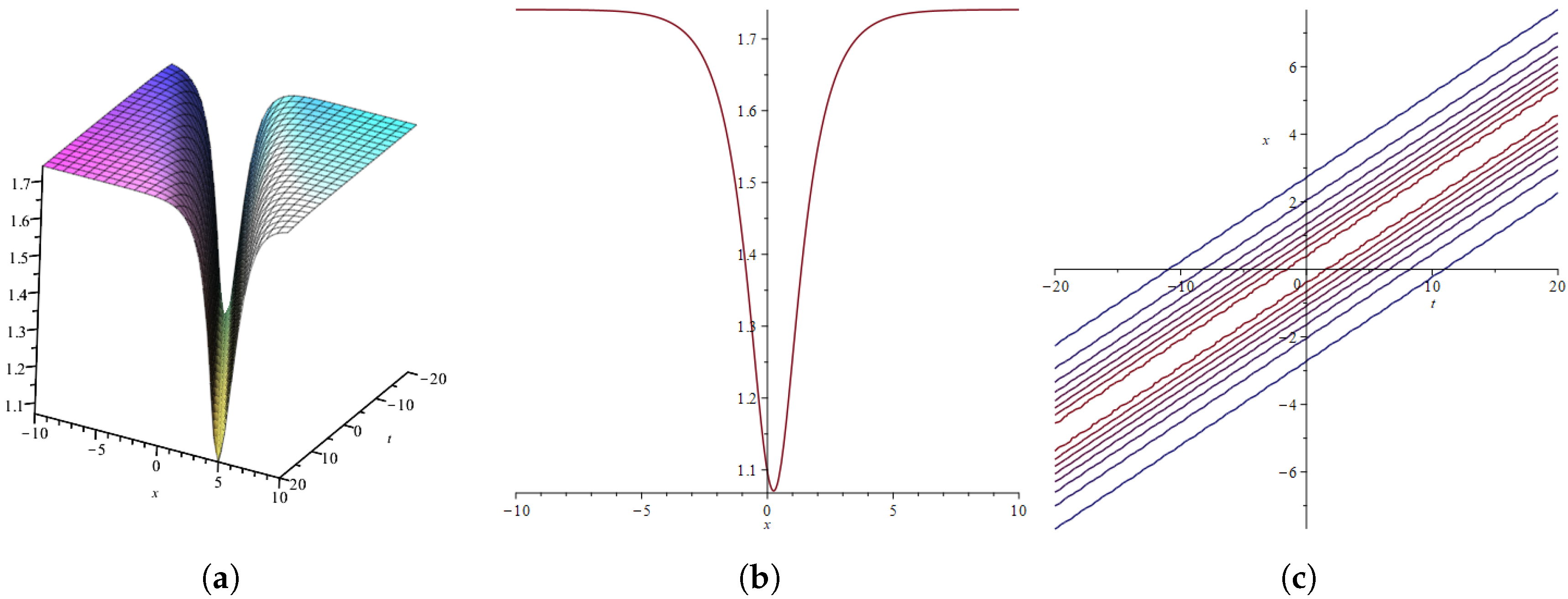
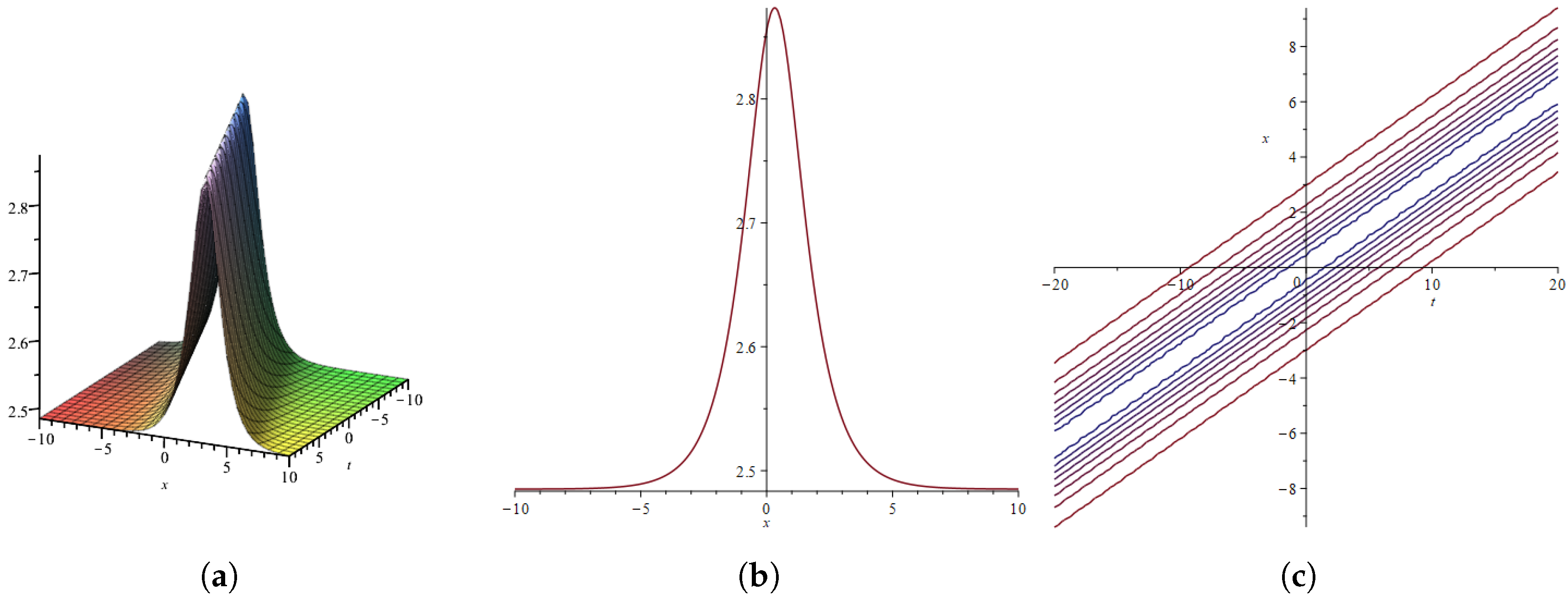
A diverse range of soliton types can be observed across different NLEE systems. For the HOKdV Equation (4), soliton solutions are present in all cases considered in this study. For instance, dark solitons (see Figure 1) are generated in ${\varphi }_{1,3.1}$ and ${\varphi }_{3,2.1}$, while bright solitons (see Figure 2) are obtained in ${\varphi }_{1,1.1}$ and ${\varphi }_{2,3.1}$. Additionally, special solitons are constructed, including the two-dark soliton in ${\varphi }_{3,1.1}$ (see Figure 3) and the bright–dark soliton in ${\varphi }_{3,3.1}$ (see Figure 4). A bright soliton is characterized as a localized wave packet with positive amplitude that remains stable within a nonlinear medium, while a dark soliton exhibits negative amplitude. A bright–dark soliton denotes the coexistence of both bright and dark soliton profiles within the same dynamical system. Finally, the two-dark soliton solution obtained here presents an interaction region rather than a full collision. As illustrated in Figure 3b, the amplitude and waveform of ${\varphi }_{3,1.1}$ remain invariant over time.

4.2. Solitary Waves and Breathers

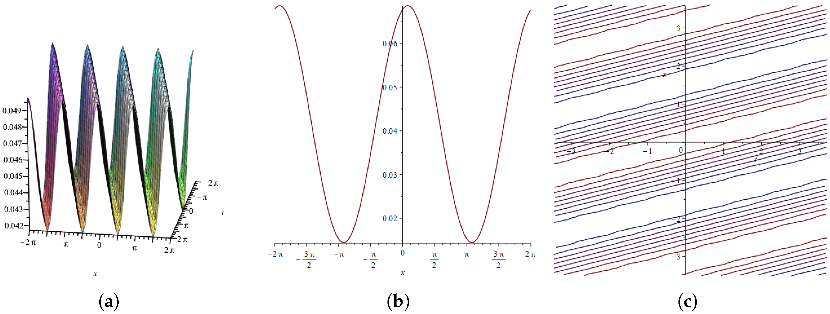
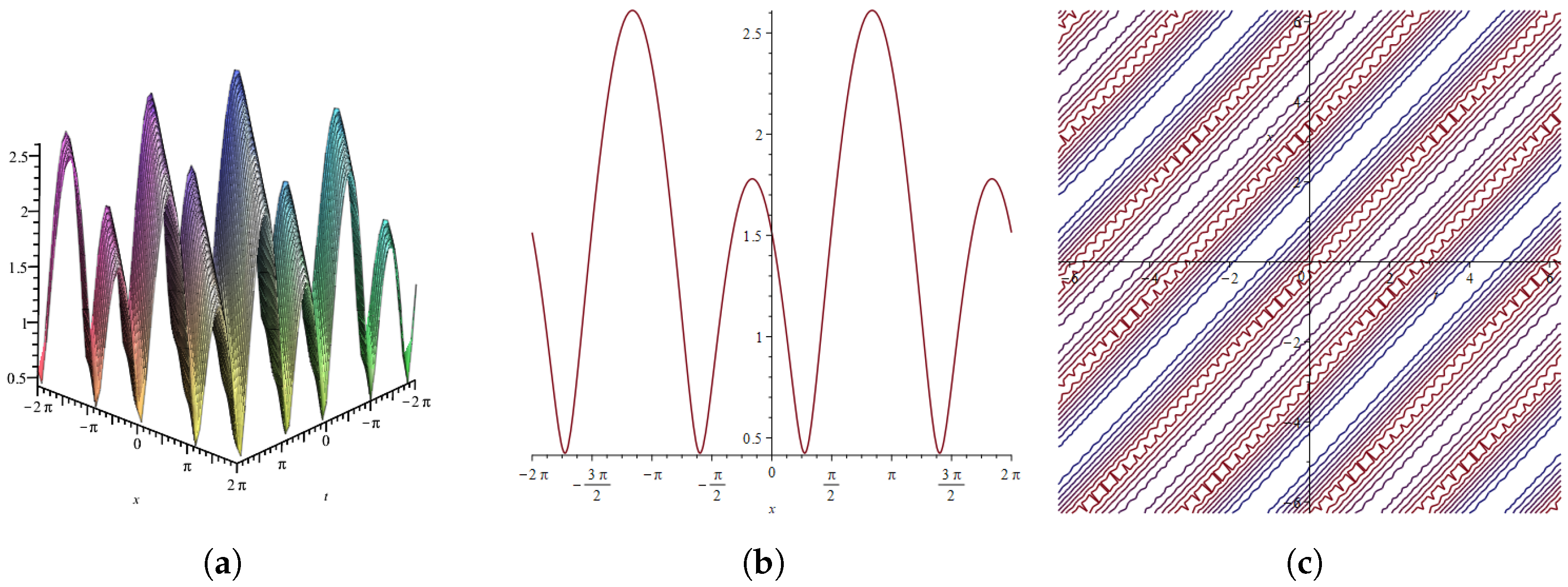
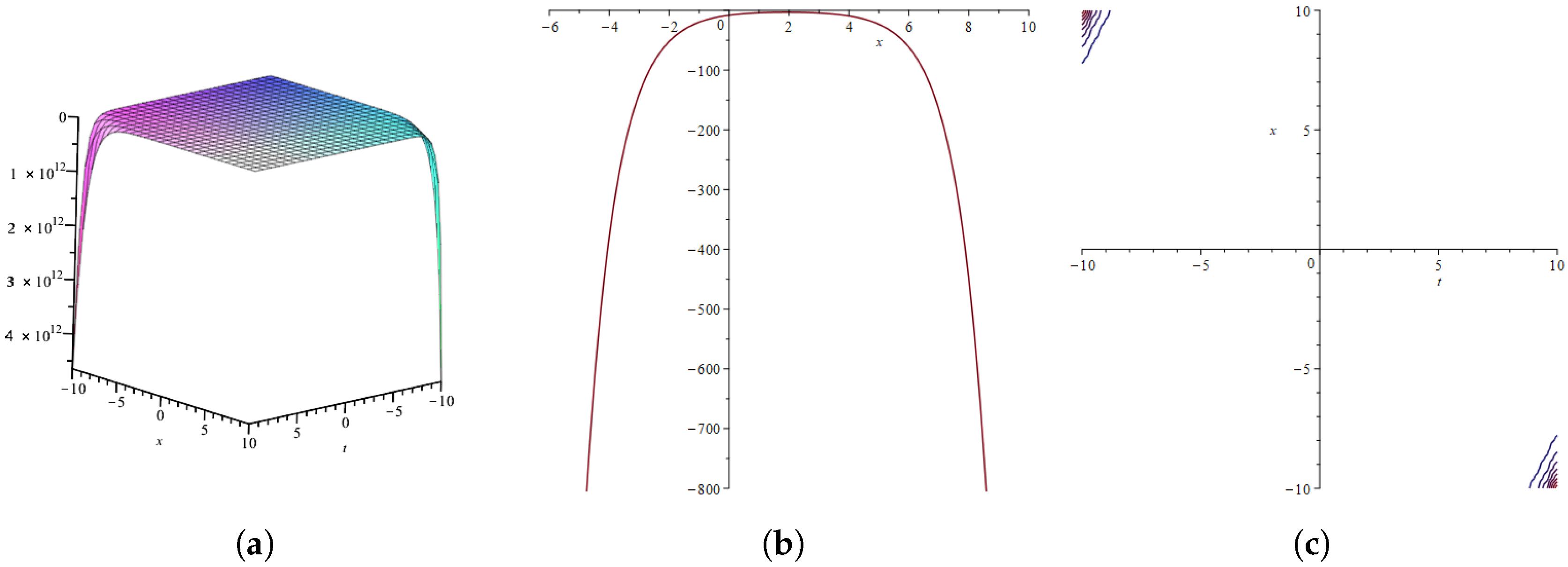
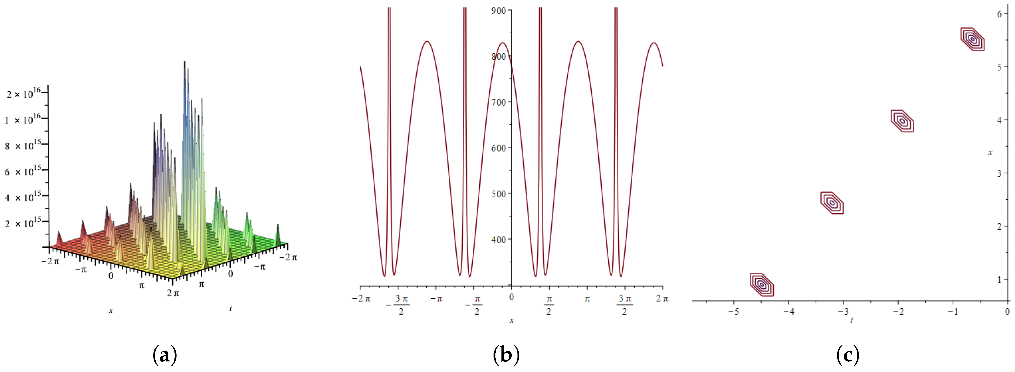
In addition to solitons, a variety of other solution types for the HOKdV Equation (4) are obtained in this work. In ${\varphi }_{1,1.2}$, ${\varphi }_{1,3.2}$, ${\varphi }_{2,2.2}$, ${\varphi }_{2,3.2}$ and ${\varphi }_{3,2.2}$, solitary wave solutions are obtained (see Figure 5 and Figure 6).These solutions are characterized by continuous, periodic waveforms with constant amplitude over time. In ${\varphi }_{2,1.1}$, a dark solitary wave is obtained (see Figure 7). In ${\varphi }_{1,2.1}$, breathers are obtained (see Figure 8), and the solution can be characterized as a set of periodic peaks or troughs, generally with uniform amplitude.

4.3. Other Intriguing Solutions

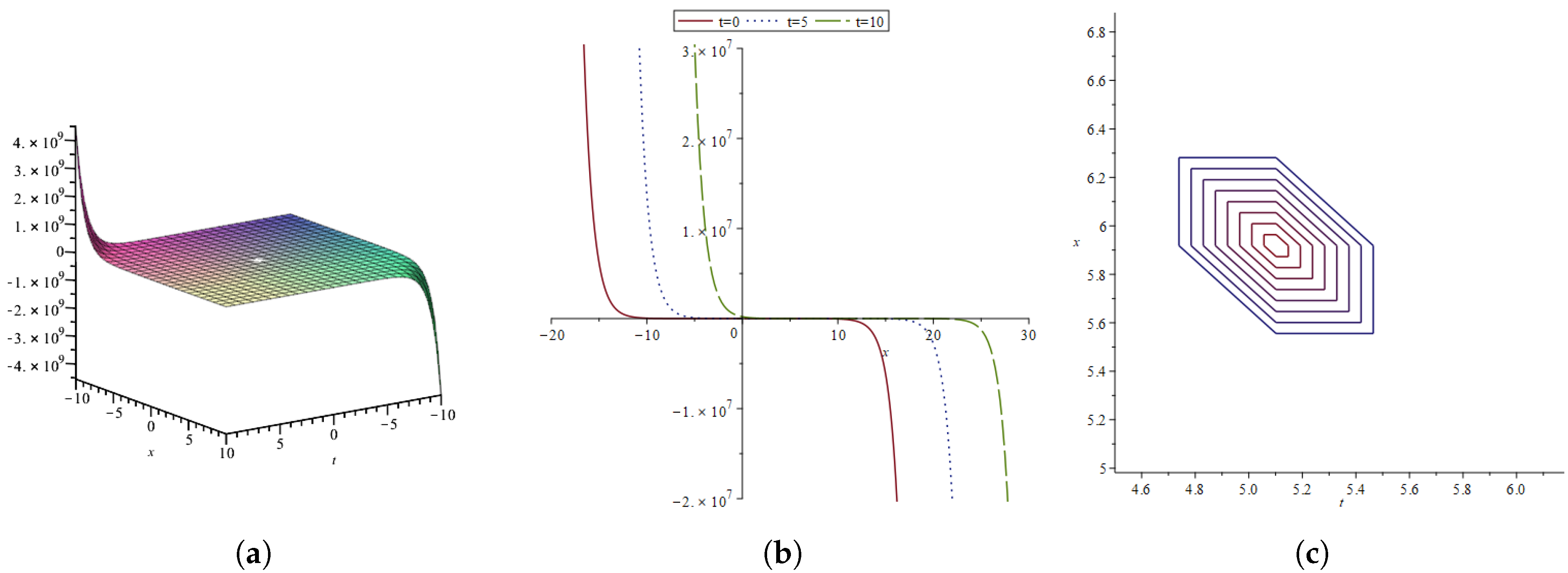
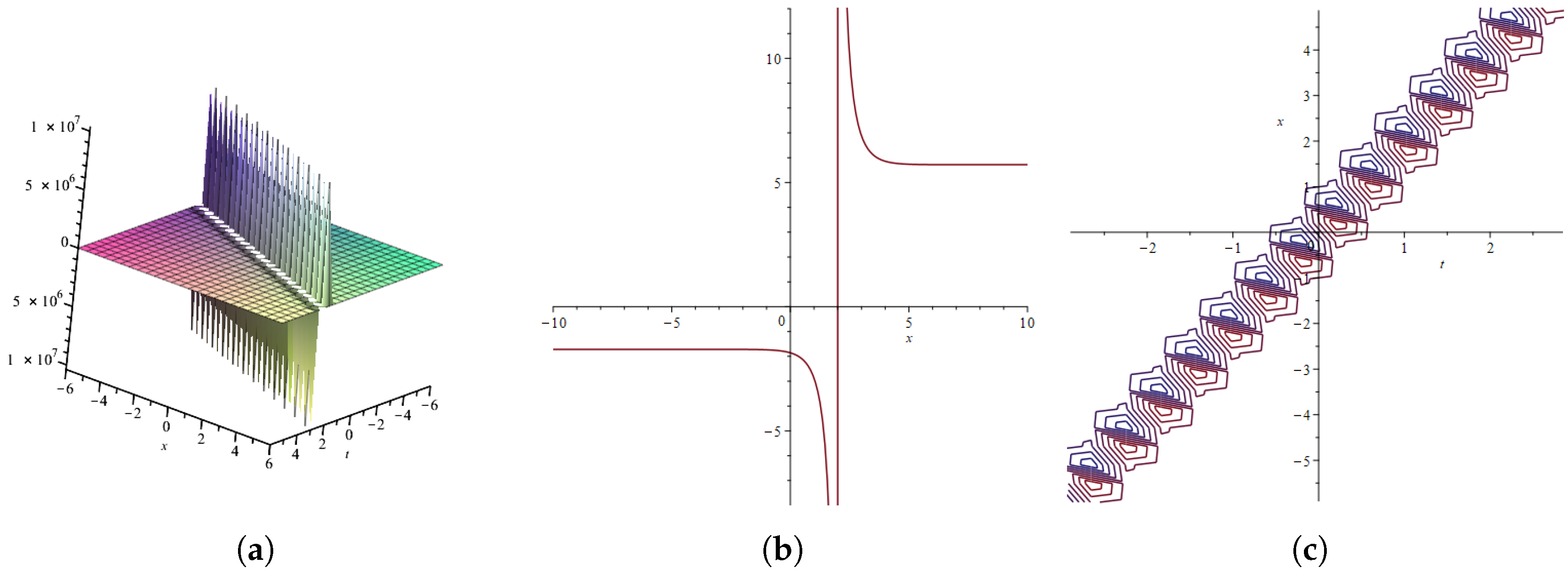
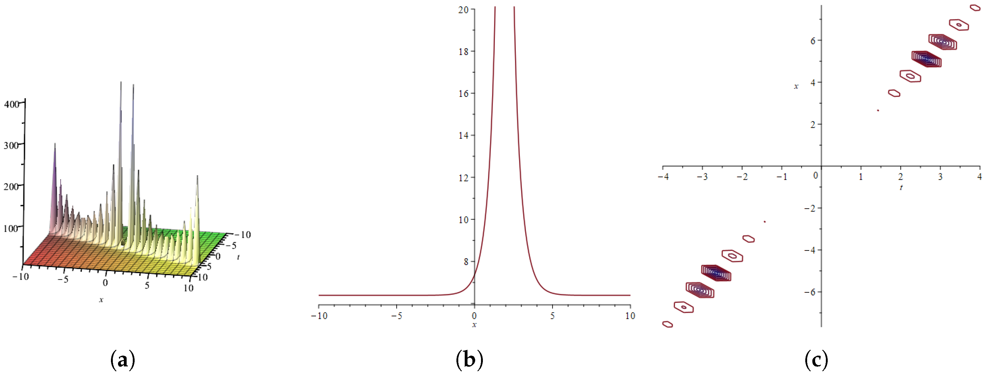
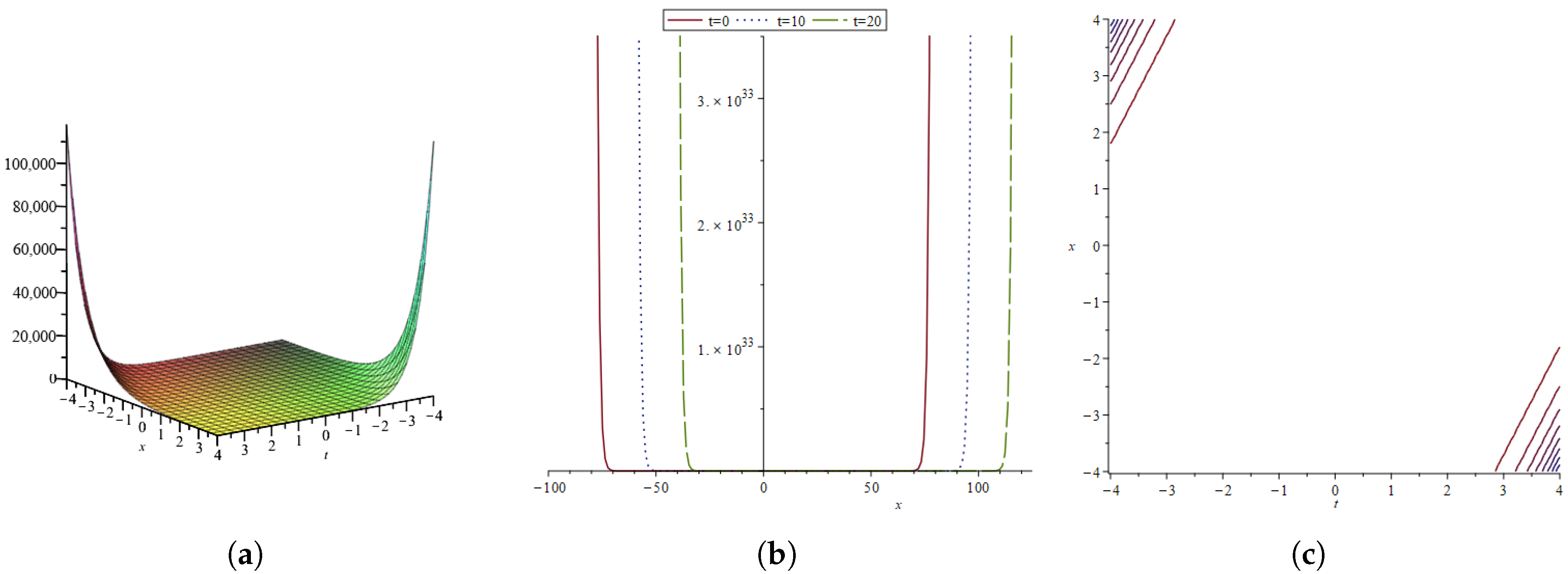
Furthermore, several solutions developed in this work exhibit interesting dynamical behaviors. Rogue-like solutions are characterized by large-amplitude localized bursts. Although their profiles do not fully match those of typical rogue wave solutions, their evolutionary patterns are highly similar. These solutions correspond to ${\varphi }_{1,2.2}$, ${\varphi }_{2,1.2}$, ${\varphi }_{3,1.2}$ and ${\varphi }_{3,3.2}$. Among these, ${\varphi }_{3,1.2}$ and ${\varphi }_{3,3.2}$ are multipeak rogue-like solutions (see Figure 9). In addition, the solution corresponding to ${\varphi }_{2,2.1}$ approaches infinity and can be regarded as extremely deep, wide and stable troughs (see Figure 10).

5. Conclusions

This paper centers on the HOKdV equation, a critical model for describing complex nonlinear wave dynamics in physical systems, and systematically investigates its exact solutions and dynamic behaviors via the extended F-expansion method.

As a preliminary and essential step, the transformation (20) is first employed to reduce the HOKdV Equation (4) to a one-dimensional ordinary differential system. Through the homogeneous balance principle (9) in conjunction with the elliptic Equation (19), the structure of Jacobi elliptic solutions for this ODE system is determined using Table 1 and Table 2 and Equation (23), establishing a rigorous mathematical foundation for subsequent solution derivation.

Three sets of Jacobi elliptic solutions are further derived by directly solving Equation (22), with the corresponding Jacobi elliptic solutions summarized in Table 3, Table 4 and Table 5. As the modulus m of Jacobi elliptic functions tends to 0 or 1, a variety of explicit solutions for Equation (22) are obtained. Via the transformation (20), corresponding explicit solutions for the HOKdV Equation (4) are constructed, encompassing dark/bright solitons, solitary waves, breathers, as well as intriguing solutions like rogue-like solutions and two-dark solitons. To characterize the nonlinear dynamics of these solutions, several representative cases are selected and visualized in three-dimensional, two-dimensional and contour plots, which offer intuitive insight into the intricate propagation characteristics governed by the HOKdV equation.

In contrast to methods such as the integral bifurcation method [33] employed in previous studies, this work, based on Kudryashov’s auxiliary equation method, provides a more unified and systematic framework for constructing Jacobi elliptic function solutions, with a greater emphasis on establishing a complete Jacobi elliptic solution hierarchy and its corresponding dynamical analysis. Furthermore, while other methods have yielded a range of solutions including soliton solutions, breather solutions, blow-up periodic wave solutions, and smooth soliton solutions, this paper generates new solution types such as dark solitary waves, rogue-like solutions and two-dark solitons, offering a complementary perspective on the solution landscape of the equation.

These results establish a theoretical foundation for understanding dynamic mechanisms in high-order nonlinear wave equations, and expand the methodological framework for solving exact solutions of nonlinear evolution equations. The construction of the Jacobi elliptic function solution system and its dynamic analysis not merely enriches the understanding of nonlinear wave propagation laws, but it also offers important references for the research on related nonlinear phenomena in fields such as fluid mechanics, plasma physics, and optics. Future research may attempt to apply the extended F-expansion method to a wider range of high-order nonlinear partial differential equations, advancing the development of nonlinear science theory and its applications.

References

1. Fokas, A.S. On a class of physically important integrable equations. Phys. D Nonlinear Phenom. 1995, 87, 145–150. [Google Scholar] [CrossRef]
2. Korteweg, D.J.; De Vries, G. XLI. On the change of form of long waves advancing in a rectangular canal, and on a new type of long stationary waves. Lond. Edinb. Dublin Philos. Mag. J. Sci. 1895, 39, 422–443. [Google Scholar] [CrossRef]
3. Fuchssteiner, B.; Fokas, A.S. Symplectic structures, their bäcklund transformations and hereditary symmetries. Phys. D Nonlinear Phenom. 1981, 4, 47–66. [Google Scholar] [CrossRef]
4. Gardner, C.S.; Greene, J.M.; Kruskal, M.D.; Miura, R.M. Method for solving the korteweg-devries equation. Phys. Rev. Lett. 1967, 19, 1095. [Google Scholar] [CrossRef]
5. Hirota, R. Exact solution of the korteweg—de vries equation for multiple collisions of solitons. Phys. Rev. Lett. 1971, 27, 1192. [Google Scholar] [CrossRef]
6. Wang, M.; Zhou, Y.; Li, Z. Application of a homogeneous balance method to exact solutions of nonlinear equations in mathematical physics. Phys. Lett. A 1996, 216, 67–75. [Google Scholar] [CrossRef]
7. Liu, S.; Fu, Z.; Liu, S.; Zhao, Q. Jacobi elliptic function expansion method and periodic wave solutions of nonlinear wave equations. Phys. Lett. A 2001, 289, 69–74. [Google Scholar] [CrossRef]
8. Malfliet, W.; Hereman, W. The tanh method: I. exact solutions of nonlinear evolution and wave equations. Phys. Scr. 1996, 54, 563. [Google Scholar] [CrossRef]
9. He, J.-H.; Wu, X.-H. Exp-function method for nonlinear wave equations. Chaos Solitons Fractals 2006, 30, 700–708. [Google Scholar] [CrossRef]
10. Lax, P.D. Integrals of nonlinear equations of evolution and solitary waves. Commun. Pure Appl. Math. 1968, 21, 467–490. [Google Scholar] [CrossRef]
11. Wang, M.; Li, X. Applications of f-expansion to periodic wave solutions for a new hamiltonian amplitude equation. Chaos Solitons Fractals 2005, 24, 1257–1268. [Google Scholar] [CrossRef]
12. Kudryashov, N.A. Exact solutions of the generalized kuramoto-sivashinsky equation. Phys. Lett. A 1990, 147, 287–291. [Google Scholar] [CrossRef]
13. Kudryashov, N. On types of nonlinear nonintegrable equations with exact solutions. Phys. Lett. A 1991, 155, 269–275. [Google Scholar] [CrossRef]
14. Kudryashov, N.A. Simplest equation method to look for exact solutions of nonlinear differential equations. Chaos Solitons Fractals 2005, 24, 1217–1231. [Google Scholar] [CrossRef]
15. Kudryashov, N.A. One method for finding exact solutions of nonlinear differential equations. Commun. Nonlinear Sci. Numer. 2012, 17, 2248–2253. [Google Scholar] [CrossRef]
16. Fan, E. Uniformly constructing a series of explicit exact solutions to nonlinear equations in mathematical physics. Chaos Solitons Fractals 2003, 16, 819–839. [Google Scholar] [CrossRef]
17. Armitage, J.V.; Eberlein, W.F. Elliptic Functions; Cambridge University Press: Cambridge, UK, 2006; Volume 67. [Google Scholar]
18. Lawden, D.F. Elliptic Functions and Applications; Springer Science & Business Media: Berlin/Heidelberg, Germany, 2013; Volume 80. [Google Scholar]
19. Bender, C.M.; Orszag, S.A. Advanced Mathematical Methods for Scientists and Engineers I: Asymptotic Methods and Perturbation Theory; Springer Science & Business Media: Berlin/Heidelberg, Germany, 2013. [Google Scholar]
20. Silambarasan, R.; Nisar, K.S. Doubly periodic solutions and non-topological solitons of 2 + 1- dimension wazwaz kaur boussinesq equation employing jacobi elliptic function method. Chaos Solitons Fractals 2023, 175, 113997. [Google Scholar] [CrossRef]
21. Ren, Y.-J.; Zhang, H.-Q. A generalized f-expansion method to find abundant families of jacobi elliptic function solutions of the (2 + 1)-dimensional nizhnik–novikov–veselov equation. Chaos Solitons Fractals 2006, 27, 959–979. [Google Scholar] [CrossRef]
22. Yan, Z. Jacobi elliptic function solutions of nonlinear wave equations via the new sinh-gordon equation expansion method. J. Phys. A Math. Gen. 2003, 36, 1961. [Google Scholar] [CrossRef]
23. Yan, Z. Abundant families of jacobi elliptic function solutions of the (2 + 1)-dimensional integrable davey–stewartson-type equation via a new method. Chaos Solitons Fractals 2003, 18, 299–309. [Google Scholar] [CrossRef]
24. Kudryashov, N.A. General solution of the traveling wave reduction for the perturbed chen-lee-liu equation. Optik 2019, 186, 339–349. [Google Scholar] [CrossRef]
25. Kudryashov, N.A. Model of propagation pulses in an optical fiber with a new law of refractive indices. Optik 2021, 248, 168160. [Google Scholar] [CrossRef]
26. Kudryashov, N.A. First integrals and solutions of the traveling wave reduction for the triki–biswas equation. Optik 2019, 185, 275–281. [Google Scholar] [CrossRef]
27. Kudryashov, N.A. First integrals and general solution of the traveling wave reduction for schrödinger equation with anti-cubic nonlinearity. Optik 2019, 185, 665–671. [Google Scholar] [CrossRef]
28. Yomba, E. The extended fan’s sub-equation method and its application to kdv–mkdv, bkk and variant boussinesq equations. Phys. Lett. A 2005, 336, 463–476. [Google Scholar] [CrossRef]
29. Xie, F.; Zhang, Y.; Lü, Z. Symbolic computation in non-linear evolution equation: Application to (3 + 1)-dimensional kadomtsev–petviashvili equation. Chaos Solitons Fractals 2005, 24, 257–263. [Google Scholar] [CrossRef]
30. Sirendaorejil; Jiong, S. Auxiliary equation method for solving nonlinear partial differential equations. Phys. Lett. A 2003, 309, 387–396. [Google Scholar] [CrossRef]
31. Farooq, A.; Khan, M.I.; Ma, W.X. Exact solutions for the improved mkdv equation with conformable derivative by using the jacobi elliptic function expansion method. Opt. Quantum Electron. 2024, 56, 542. [Google Scholar] [CrossRef]
32. He, Y.; Zhao, Y.-M.; Long, Y. New exact solutions for a higher-order wave equation of kdv type using extended f-expansion method. Math. Probl. Eng. 2013, 2013, 128970. [Google Scholar] [CrossRef]
33. Rui, W. Exact solutions of a high-order nonlinear wave equation of korteweg-de vries type under newly solvable conditions. In Abstract and Applied Analysis; Wiley Online Library: Hoboken, NJ, USA, 2014; Volume 2014, p. 714214. [Google Scholar]
Figure 1. (a) Three-dimensional surface plot, (b) two-dimensional plot and (c) contour plot for the dark soliton ϕ 1 , 3.1 by selecting ρ 1 = 0.8 , ρ 3 = 1 , α = β = 0.8 , t = 1 .
Mathematics 14 00886 g001
Figure 2. (a) Three-dimensional surface plot, (b) two-dimensional plot and (c) contour plot for the bright soliton ϕ 2 , 3.1 by selecting ρ 1 = 1 , ρ 3 = 1.2 , α = β = 0.8 , R = 1 , t = 1 .
Mathematics 14 00886 g002
Figure 3. (a) Three-dimensional surface plot, (b) two-dimensional plot and (c) unilateral contour plot for the two-dark soliton ϕ 3 , 1.1 by selecting A 0 = 0.8 , R = 2 , α = 0.4 , β = 0.6 , t = 1 .
Mathematics 14 00886 g003
Figure 4. (a) Three-dimensional surface plot, (b) two-dimensional plot and (c) contour plot for the bright–dark soliton ϕ 3 , 3.1 by selecting A 0 = 2 , R = 1 , α = 1 , β = 0.6 , t = 1 .
Mathematics 14 00886 g004
Figure 5. (a) Three-dimensional surface plot, (b) two-dimensional plot and (c) contour plot for the solitary wave ϕ 1 , 1.2 by selecting ρ 1 = 1 , ρ 3 = 2 , α = β = 0.8 , t = 1 .
Mathematics 14 00886 g005
Figure 6. (a) Three-dimensional surface plot, (b) two-dimensional plot and (c) contour plot for the solitary wave ϕ 3 , 2.2 by selecting A 0 = 0.6 , R = 2 , α = 0.2 , β = 1 , t = 1 .
Mathematics 14 00886 g006
Figure 7. (a) Three-dimensional surface plot, (b) two-dimensional plot and (c) contour plot for the dark solitary wave ϕ 2 , 1.1 by selecting ρ 1 = 1 , ρ 3 = 1.2 , α = β = 0.8 , R = 1 , t = 1 .
Mathematics 14 00886 g007
Figure 8. (a) Three-dimensional surface plot, (b) two-dimensional plot and (c) contour plot for the breathers ϕ 1 , 2.1 by selecting ρ 1 = 0.2 , ρ 3 = 1 , α = 0.6 , β = 0.8 , t = 1 .
Mathematics 14 00886 g008
Figure 9. (a) Three-dimensional surface plot, (b) two-dimensional plot and (c) contour plot for the rogue-like solution ϕ 3 , 3.2 by selecting A 0 = 2 , R = 1 , α = 0.2 , β = 0.8 , t = 1 .
Mathematics 14 00886 g009
Figure 10. (a) Three-dimensional surface plot, (b) two-dimensional plot and (c) contour plot for the solution tends to infinity ϕ 2 , 2.1 by selecting ρ 1 = 0.4 , ρ 3 = 1.2 , α = 0.6 , β = 0.8 , t = 0 , 10 , 20 .
Mathematics 14 00886 g010