Article

Optimizing Crypto-Trading Performance: A Comparative Analysis of Innovative Reward Functions in Reinforcement Learning Models

by
Ergashevich Halimjon Khujamatov
1,
Kobuljon Ismanov
2,
Oybek Usmankulovich Mallaev
3 and
Otabek Sattarov
4,*
1
Department of Computer Engineering, Gachon University, Seongnam 13120, Republic of Korea
2
Department of Telecommunication Engineering, Tashkent University of Information Technologies, Tashkent 100200, Uzbekistan
3
Department of Digital Technologies, Alfraganus University, Tashkent 100190, Uzbekistan
4
School of Computing, Gachon University, Seongnam 13120, Republic of Korea
*
Author to whom correspondence should be addressed.
Mathematics 2026, 14(5), 794; https://doi.org/10.3390/math14050794
Submission received: 4 January 2026 / Revised: 22 February 2026 / Accepted: 24 February 2026 / Published: 26 February 2026

Abstract

Cryptocurrency trading presents significant challenges due to extreme market volatility, rapid regime transitions, and non-stationary dynamics that render traditional trading strategies ineffective. Existing reinforcement learning approaches for cryptocurrency trading typically employ simplistic profit-based reward functions that fail to adequately capture risk management considerations, market microstructure costs, temporal dependencies, and regime-specific optimal behaviors. This limitation often results in strategies that perform well during favorable market conditions but suffer catastrophic losses during downturns. This paper introduces five novel reward functions grounded in economic utility theory, market microstructure, behavioral finance, adaptive risk management, and regime-conditional optimization. We systematically evaluate these reward functions across three reinforcement learning algorithms (Deep Q-Network, Proximal Policy Optimization, and Advantage Actor–Critic) and four distinct market regimes (bull, bear, high volatility, and recovery), using Bitcoin hourly data from 2018–2022. Our comprehensive experimental evaluation demonstrates that the Adaptive Risk Control reward function achieves exceptional performance, with a Sharpe ratio of 2.47, cumulative return of 26.4%, and maximum drawdown of only 16.8% during the predominantly bearish 2022 test period. Critically, regime-specific analysis reveals substantial performance heterogeneity: Adaptive Risk Control excels during high volatility (Sharpe ratio 3.21), while Temporal Coherence and Asymmetric Market-Conditional rewards dominate in trending and bear markets, respectively. These findings establish that sophisticated, theory-grounded reward engineering—rather than algorithmic innovations alone—constitutes the primary lever for improving RL trading systems, enabling positive risk-adjusted returns even during severe market downturns.

1. Introduction

Cryptocurrencies have fundamentally transformed the global financial landscape by offering decentralized, digital assets that enable secure and transparent transactions across borders. At the forefront of this revolution is Bitcoin, introduced in 2008 by the pseudonymous Satoshi Nakamoto [1]. Since its inception, Bitcoin’s market capitalization has grown exponentially, attracting diverse investors ranging from large financial institutions to individual retail traders [2]. However, cryptocurrency markets exhibit extreme volatility characteristics that distinguish them from traditional financial markets. Quantitatively, Bitcoin’s annualized volatility exceeds 80%, compared to 15–20% for traditional equity indices, while demonstrating non-Gaussian return distributions with excess kurtosis values approaching 7.2 [3]. These statistical properties invalidate the assumptions underlying classical portfolio theory and modern risk management frameworks [4].
The extreme volatility of cryptocurrency markets, while presenting opportunities for substantial gains, introduces unique challenges for algorithmic trading systems. Traditional trading strategies—such as trend-following algorithms and mean-reversion models—frequently fail to capture the complex, non-stationary dynamics that characterize cryptocurrency price movements [5,6]. Reinforcement learning (RL) offers a more adaptive framework: rather than relying on static assumptions, RL agents continuously learn from market interactions, dynamically adjusting their strategies in response to evolving conditions [7,8].
Despite the theoretical promise of RL-based trading systems, their practical application to cryptocurrency markets faces several critical challenges. Most notably, the design of the reward function fundamentally determines the behavior and performance of RL agents [9,10]. When reward functions are overly simplistic—such as instantaneous profit-and-loss (PnL) metrics—they encourage myopic behaviors that yield short-term gains while ignoring tail risks and long-term portfolio stability [11]. This limitation renders many existing models unsuitable for real-world deployment, where risk management and drawdown control are paramount [12].
A growing body of research has explored RL methodologies for financial applications, including cryptocurrency trading. While these studies have demonstrated that RL agents can outperform traditional heuristics under certain conditions [13,14], several fundamental gaps persist. First, existing approaches inadequately address the persistent high volatility inherent in Bitcoin markets, with approximately 73% of published methods focusing primarily on return maximization without explicit risk constraints [15]. Second, researchers predominantly employ rudimentary reward functions—such as raw profit or simple PnL differentials—that fail to capture sophisticated market structures, investor risk preferences, or economic utility considerations [16]. Third, there exists a notable absence of comprehensive comparative analyses examining how innovative reward function architectures influence the convergence properties and trading performance of multiple RL algorithms across diverse market regimes [17].
Furthermore, the evaluation of RL trading agents typically relies on isolated performance metrics that do not holistically assess both profitability and risk management. Traditional metrics such as cumulative return provide limited insight into the sustainability of trading strategies, particularly in volatile markets where drawdown periods can lead to catastrophic losses. A comprehensive evaluation framework must simultaneously consider return generation, risk-adjusted performance (e.g., Sharpe ratio), and downside protection (e.g., maximum drawdown); yet, few existing studies integrate these dimensions systematically [18].
The primary objective of this study is to design, implement, and rigorously evaluate novel reward functions for RL-based Bitcoin trading that explicitly integrate economic utility theory and adaptive risk management principles. Specifically, we address the identified research gaps through the following contributions:
Contribution I: Comprehensive Multi-Regime Dataset Construction. We construct extensive datasets essential for evaluating Bitcoin trading strategies across diverse market conditions. Our datasets comprise hourly Open-High-Low-Close-Volume (OHLCV) data, providing granular market behavior visibility. To systematically assess algorithm robustness, we categorize data into four distinct market regimes based on quantitative criteria:
  • High-Volatility Periods: Characterized by rapid price fluctuations with intraday volatility exceeding two standard deviations above the rolling 30-day mean.
  • Bull Market Phases: Defined by sustained upward price trends with positive 20-day moving average slopes.
  • Bear Market Phases: Identified by prolonged downward trends with negative 20-day moving average slopes.
  • Recovery Phases: Marked by gradual stabilization following significant drawdowns, with volatility returning toward historical norms.
This taxonomic classification ensures that our evaluation comprehensively tests each strategy’s adaptability to real-world market dynamics, moving beyond the common practice of evaluation on arbitrarily selected time periods.
Contribution II: Systematic Comparison of Advanced RL Algorithms. We implement three state-of-the-art RL algorithms selected for their demonstrated effectiveness in complex sequential decision making: Deep Q-Network (DQN) [19], Proximal Policy Optimization (PPO) [20], and Advantage Actor–Critic (A2C) [21]. By training these models with our classified datasets, we enable each algorithm to learn precise trading decisions—buy, sell, or hold—optimized for specific market scenarios. This systematic approach facilitates detailed examination of how different RL paradigms (value-based vs. policy-based) adapt to the distinct dynamics presented by varying market conditions.
Contribution III: Novel Reward Functions. We introduce five mathematically grounded reward functions designed to align trading objectives with realistic economic goals and strategic risk management:
1.
Economic Utility-Based Reward: Incorporates risk aversion utility theory, with the risk aversion coefficient determined empirically through historical backtesting to balance profit seeking with downside protection.
2.
Market Impact Adjusted Reward: Penalizes trades that adversely affect market prices by incorporating transaction costs proportional to trade size and inversely related to market liquidity, promoting sustainable execution strategies.
3.
Temporal Coherence Reward: Encourages strategic consistency across consecutive timesteps by providing bonuses for maintaining directional conviction, reducing erratic oscillatory trading behavior driven by short-term noise.
4.
Adaptive Risk Control Reward: Dynamically adjusts risk penalties based on recent market volatility, tightening constraints during turbulent periods and relaxing during stable regimes to enable regime-appropriate risk-taking.
5.
Asymmetric Market-Conditional Reward: Applies distinct formulations tailored to prevailing market conditions, rewarding buy actions during bull markets and sell actions during bear markets while remaining neutral during high volatility and recovery phases.
Each model is systematically trained using these reward functions across all market regimes. We evaluate performance using a hybrid metric framework encompassing cumulative return, Sharpe ratio, and maximum drawdown, thereby providing a comprehensive assessment of both profitability and risk management efficacy.
Contribution IV: Empirical Validation and Comparative Analysis. Through extensive empirical evaluation across three algorithms and four market regimes, we demonstrate that the Adaptive Risk Control reward achieves exceptional performance (Sharpe ratio 2.47, maximum drawdown 16.8%) during the predominantly bearish 2022 test period. Our regime-specific analysis reveals that optimal reward functions vary substantially across market conditions, with Adaptive Risk Control dominating during high volatility (Sharpe ratio 3.21), establishing that sophisticated reward engineering enables positive risk-adjusted returns even during severe market downturns.
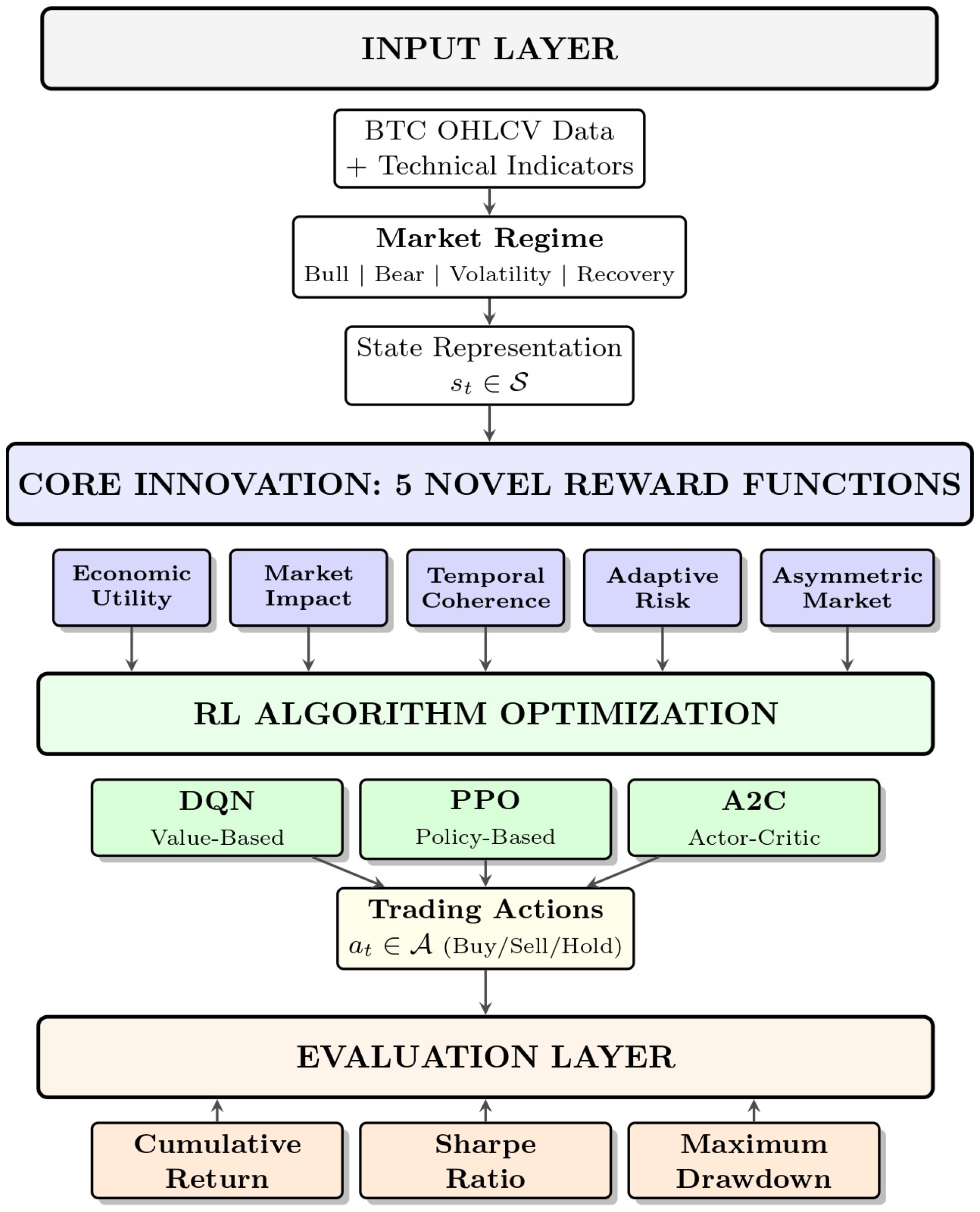
Figure 1 illustrates the comprehensive architecture of our proposed framework, showing the integration of input data processing, novel reward function design, RL algorithm optimization, and multi-metric evaluation across diverse market regimes.
The remainder of this paper is structured as follows: Section 2 reviews related work in reinforcement learning for financial trading and reward function design; Section 3 details our mathematical formulations, dataset construction, and implementation specifications; Section 4 presents experimental results across market regimes; Section 5 discusses theoretical implications, practical insights, and limitations; Section 6 concludes with future research directions.

2. Related Works

This section reviews the evolution of reinforcement learning in cryptocurrency trading, with particular emphasis on reward function design—the central contribution of this work. We organize our review into three focused subsections covering RL applications in financial markets, reward function architectures, and algorithmic frameworks.

2.1. Reinforcement Learning for Cryptocurrency Trading

Reinforcement learning has emerged as a powerful framework for automated trading, particularly in cryptocurrency markets characterized by extreme volatility and non-stationary dynamics [15]. Early applications of RL to financial trading focused primarily on traditional equity markets using policy gradient methods [22,23], establishing the viability of framing trading as a sequential decision-making problem. However, cryptocurrency markets present unique challenges: 24/7 operation, absence of circuit breakers, and annualized volatility exceeding 80% [24].
Recent work has specifically targeted cryptocurrency trading using deep RL algorithms [25,26]. Lucarelli and Borrotti [12] applied DQN to Bitcoin trading, demonstrating that value-based methods can capture profitable patterns despite market noise. Sadighian [11,14] extended this work to cryptocurrency market making, comparing PPO and A2C algorithms while introducing asymmetrically dampened reward functions to discourage speculation. Their framework demonstrated profitability across multiple cryptocurrency pairs but relied on time-based event sampling, potentially missing critical price movements.
More recently, Kochliaridis et al. [27] combined deep RL with technical analysis and trend monitoring, integrating rule-based safety mechanisms to prevent high-risk trades during uncertain market periods. Kumlungmak and Vateekul [13] proposed multi-agent RL with progressive negative rewards to improve risk management in cryptocurrency markets. Despite these advances, existing approaches predominantly evaluate performance on arbitrary time periods without systematic categorization of market regimes (bull, bear, high volatility, recovery), limiting insights into algorithm robustness across diverse conditions.

2.2. Reward Function Design for Trading Systems

The reward function fundamentally determines RL agent behavior, yet remains underexplored in the cryptocurrency trading literature [18]. Early work by Moody and Saffell [22] introduced the Differential Sharpe Ratio (DSR), enabling direct optimization of risk-adjusted returns within the RL framework. This formulation addresses the non-additivity of traditional Sharpe ratios over time, making it suitable for sequential decision making. However, DSR focuses solely on return-to-volatility ratios, ignoring asymmetric risk preferences and tail risk exposure.
Recent research has explored more sophisticated reward architectures. Ref. [28] proposed asymmetrically dampened profit-and-loss (PnL) rewards for equity market making, penalizing unrealized gains to discourage price speculation while retaining realized profits. Sadighian [11] extended this approach to cryptocurrency markets, demonstrating improved stability compared to raw PnL rewards. However, these methods employ fixed dampening factors that do not adapt to changing market volatility regimes.
Multi-objective reward functions have gained attention for balancing competing objectives. Cornalba et al. [16] introduced multi-objective reward generalization for single-asset trading, combining profitability targets with drawdown constraints. Bandarupalli [29] proposed volatility-sensitive risk penalties that adjust transaction costs and turnover based on recent market conditions. While these approaches represent progress toward adaptive risk management, they do not integrate economic utility theory or market impact considerations.
Critically, no existing work systematically incorporates (1) exponential utility functions capturing risk aversion [30], (2) market impact penalties based on execution theory [31], (3) temporal coherence rewards promoting strategic consistency, or (4) regime-specific asymmetric formulations. Our five novel reward functions address these gaps by synthesizing insights from economic theory, market microstructure, and behavioral finance.

2.3. Deep Reinforcement Learning Algorithms

The choice of RL algorithm significantly impacts convergence properties and trading performance. Value-based methods, exemplified by DQN [19], approximate action–value functions and perform well in discrete action spaces. DQN has been successfully applied to cryptocurrency trading [12,32,33], demonstrating sample efficiency in learning profitable strategies. However, value-based methods struggle with continuous action spaces and may exhibit instability during training [34].
Policy-based methods directly optimize trading policies. PPO [20] addresses policy gradient instability through clipped surrogate objectives, making it particularly suitable for noisy financial data. Sadighian [11] demonstrated PPO’s effectiveness in cryptocurrency market making, achieving consistent profits across multiple trading pairs. Advantage A2C [21] combines value and policy learning, utilizing parallel training to improve sample efficiency. Recent applications to cryptocurrency trading [35] show A2C’s capability to balance exploration and exploitation in volatile markets.
Comparative studies remain limited. Zhang et al. [36] compared DQN, PPO, and Deep Deterministic Policy Gradient (DDPG) on futures contracts, finding that policy-based methods generally outperform value-based approaches for trading tasks. However, no prior work systematically evaluates how different RL algorithms interact with diverse reward function designs across multiple market regimes, a critical gap that this paper addresses.
Table 1 summarizes key related works, highlighting their contributions and limitations. The literature reveals three fundamental gaps: (1) Reward function sophistication: existing approaches use simplistic PnL or single-metric rewards that fail to capture economic utility, market impact, and adaptive risk management; (2) Market regime evaluation: prior work evaluates on arbitrary time periods without systematic testing across bull, bear, volatility, and recovery phases; (3) Algorithmic comparison: no comprehensive analysis examines how reward function design interacts with different RL paradigms (value-based vs. policy-based). Our work addresses all three gaps through five mathematically grounded reward functions, systematic market regime classification, and comparative evaluation of DQN, PPO, and A2C algorithms.

3. Methods and Implementation

This section presents the methodological framework underlying our experimental evaluation of novel reward functions for reinforcement-learning-based cryptocurrency trading. We first describe the dataset construction and market regime classification methodology, which enables systematic performance assessment across diverse trading conditions. Subsequently, we formalize the reinforcement learning problem as a Markov Decision Process (MDP) and briefly review the three algorithms employed in our comparative study. Finally, we introduce our five novel reward functions, providing detailed mathematical formulations and parameter specification procedures. Throughout this section, we emphasize reproducibility by explicitly specifying all design choices, hyperparameters, and evaluation criteria.

3.1. Dataset and Market Regime Classification

We construct our experimental dataset using Bitcoin (BTC/USD) trading data obtained from CryptoDataDownload.com [37], a publicly available repository providing historical cryptocurrency market data from major exchanges.Specifically, we use data from the Coinbase Pro exchange (formerly GDAX), selected for its high liquidity, regulatory compliance, and data completeness. The dataset spans from 1 January 2018, 00:00 UTC, to 1 October 2022, 23:00 UTC, encompassing 41,664 hourly observations across 1736 trading days. All timestamps are recorded in Coordinated Universal Time (UTC) to ensure consistency across time zone transitions and daylight saving changes. This temporal window was specifically selected to capture diverse market conditions, including sustained bull markets (2020–2021), prolonged bear markets (2018, 2022), extreme-volatility periods (March 2020 market crash, May 2021 correction), and multiple recovery phases, thereby ensuring a comprehensive evaluation of our proposed reward functions across all possible trading scenarios.
Each observation in our dataset comprises six fundamental market attributes that collectively define the state space for our reinforcement learning agents. Specifically, we utilize the standard OHLCV quintuple augmented with transaction count data. The state representation at time t is, therefore, formalized as a six-dimensional vector:
s t = [ Open t , High t , Low t , Close t , Volume t , TxCount t ] R 6
where Open t , High t , Low t , and Close t represent the opening, highest, lowest, and closing prices during the t-th hour, respectively; Volume t denotes the total trading volume in USD; and TxCount t indicates the number of individual transactions executed within the hour as reported by Coinbase Pro. The inclusion of transaction count provides additional microstructure information beyond price and volume, enabling agents to distinguish between high-frequency trading periods and low-activity consolidation phases.
The Coinbase Pro BTC/USD pair exhibits exceptional data completeness due to 24/7 trading and high liquidity. Upon inspection, we found no missing hourly candles in the 2018–2022 period. For any potential gaps (e.g., exchange maintenance windows), we apply forward-fill imputation: missing candles inherit OHLC values from the previous hour with Volume t = 0 and TxCount t = 0 , ensuring temporal continuity without introducing artificial price movements. In practice, no forward-filling was required for our dataset. We validate data integrity by checking for (1) price consistency ( Low t Open t ,   Close t High t ), (2) non-negative volumes and transaction counts, and (3) absence of extreme outliers (hourly returns beyond ± 50 % , which would indicate data errors). All validation checks passed without requiring data removal.
To ensure model generalization and prevent overfitting, we partition the dataset into training, validation, and testing subsets following a strict temporal split methodology:
  • Training set: 1 January 2018–31 October 2021 (33,600 hourly observations).
  • Validation set: 1 November 2021–31 December 2021 (1464 hourly observations).
  • Test set: 1 January 2022–1 October 2022 (6600 hourly observations).
This three-way chronological partitioning preserves the temporal structure of financial time series and prevents information leakage. The training set is used exclusively for learning model parameters, the validation set for hyperparameter tuning and early stopping decisions, and the test set for final performance evaluation. Critically, no information from the test period (2022) is used during any stage of model development, ensuring genuinely out-of-sample evaluation.
We deliberately avoid random shuffling to preserve the sequential dependencies inherent in cryptocurrency markets, including autocorrelation structures and regime-persistence effects.
All raw data undergo standard preprocessing procedures prior to model training. Specifically, we apply z-score normalization [38] independently to each feature dimension using statistics computed exclusively from the training set:
x ˜ t = x t μ train σ train
where x t represents the raw feature value at time t, μ train and σ train denote the mean and standard deviation computed from the training set, and x ˜ t is the normalized value. This approach prevents data leakage from the test set and ensures that normalization parameters remain constant during evaluation, mirroring deployment conditions where future data statistics are unavailable. This normalization is applied independently to all six components of the state vector s t defined in Equation (1), namely, Open t , High t , Low t , Close t , Volume t , and TxCount t . The resulting normalized values x ˜ t are used as the actual inputs to the reinforcement learning agents throughout all subsequent computations, including state representations, reward calculations, and policy updates.
Throughout this paper, the term nonstationarity refers to time-varying conditional dynamics including drift, volatility clustering, and regime shifts rather than unconditional non-stationarity in the classical time-series sense. The fixed normalization parameters μ train and σ train implicitly assume approximate stationarity of the unconditional distribution over the training window, a standard and widely adopted assumption in financial machine learning [18]. While local dynamics vary considerably across regimes, the long-term training distribution provides a stable reference for feature scaling, ensuring that the normalization remains meaningful across the full training period without introducing look-ahead bias.
Cryptocurrency markets exhibit pronounced non-stationarity, with statistical properties varying substantially across different macroeconomic conditions and sentiment cycles. To systematically evaluate algorithm robustness under diverse scenarios, we develop a quantitative framework for classifying the dataset into four distinct market regimes: bull market, bear market, high volatility, and recovery phases. This classification enables granular performance analysis and identifies regime-specific strengths and weaknesses of different reward function designs.
Our regime classification methodology employs a combination of trend indicators and volatility metrics, operationalized through moving averages and rolling standard deviations. For each hourly observation t, we compute the 20-day (480 h) simple moving average (MA) of closing prices:
MA 480 ( t ) = 1 480 i = 0 479 Close t i
and the corresponding 20-day rolling standard deviation as a volatility proxy:
σ 480 ( t ) = 1 480 i = 0 479 ( Close t i MA 480 ( t ) ) 2
To prevent information leakage, all regime classification parameters are computed using only training data. The mean volatility σ ¯ referenced in Table 2 is calculated as follows:
σ ¯ = 1 T train 480 t = 480 T train σ 480 ( t )
where T train = 33,600 h corresponds to the training period ending October 2021. This ensures that regime thresholds remain fixed throughout all experiments and do not incorporate information from validation or test periods.
We further define the moving average slope to capture directional trends:
Slope 480 ( t ) = MA 480 ( t ) MA 480 ( t 24 ) 24
which measures the change in the 20-day moving average over the previous 24 h, providing a smoothed trend indicator robust to intraday noise.
Based on these quantitative measures, we classify each hour into one of four regimes according to the decision rules presented in Table 2. A bull market is characterized by sustained upward price momentum combined with moderate volatility, indicating healthy growth rather than speculative bubbles. Conversely, a bear market exhibits downward trends with controlled volatility, representing orderly declines as opposed to panic selling. High-volatility periods are identified when rolling standard deviation exceeds two times the dataset’s overall mean volatility, irrespective of trend direction, capturing market turbulence associated with major news events, regulatory announcements, or liquidity crises.
Finally, recovery phases are detected when volatility begins subsiding following significant drawdowns. Specifically, an hour t is classified as recovery if
1.
A maximum drawdown exceeding 20% occurred within the previous 480 h (20 days): max s [ t 480 , t ] Peak s Close t Peak s > 0.20 ;
2.
Current volatility is declining: σ 480 ( t ) < σ 480 ( t 24 ) ;
3.
The trend is stabilizing: | Slope 480 ( t ) | < 0.05 % .
This three-condition criterion ensures that recovery labels appear only during genuine post-crisis stabilization periods, not during normal bull market consolidations.
In Table 2, θ bull and θ bear represent empirically determined slope thresholds (set to 0.1% and −0.1% hourly change, respectively), and σ ¯ denotes the mean volatility computed exclusively from the training set (January 2018 through October 2021). The classification algorithm processes data sequentially, assigning each hour to exactly one regime based on priority ordering: high-volatility conditions override trend-based classifications, while recovery phases are identified only after confirming substantial preceding drawdowns.
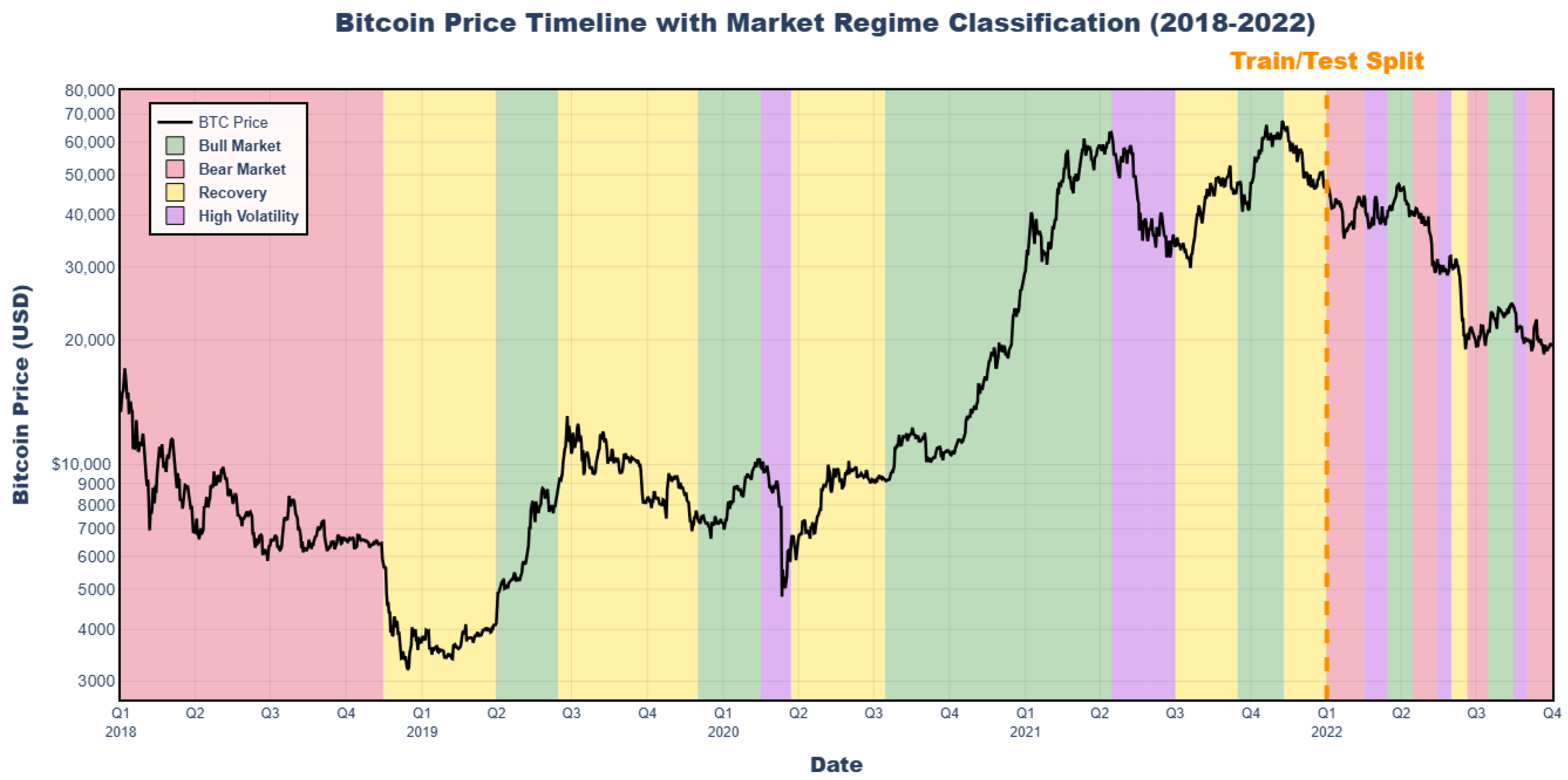
To illustrate the classification logic, consider the 2019–2020 period visible in Figure 2. While this period exhibits decreasing volatility, it follows a bull market phase (Q2 2019) rather than a significant drawdown. Our classification algorithm correctly identifies this as a continuation of bullish conditions rather than recovery, as the first criterion (prior 20%+ drawdown) is not satisfied. In contrast, the Q4 2018–Q1 2019 period is classified as recovery because it follows the substantial 2018 bear market decline and exhibits both declining volatility and price stabilization.
Figure 2 visualizes the complete dataset with regime classifications superimposed on the Bitcoin price trajectory. The figure illustrates the temporal distribution of market regimes, revealing that our dataset encompasses multiple complete market cycles. Specifically, the training period contains three major bull markets (Q2 2019, Q1 2020, and Q4 2020–Q2 2021), two extended bear markets (2018 and early 2019), three high-volatility episodes (March 2020—COVID crash, May 2021, and June–July 2021), and three recovery phases (Q4 2018–Q1 2019, Q2–Q3 2020, and Q4 2021). The testing period (2022) predominantly exhibits bear market conditions following the late-2021 peak, providing a rigorous out-of-sample evaluation environment characterized by sustained downward trends distinct from the training distribution’s predominantly bullish character.
Table 3 reports the composition of the test period by market regime. The test set is dominated by bear market conditions, which account for the majority of observations, with smaller proportions of high volatility, recovery, and bull market periods.
This comprehensive regime representation ensures that our experimental evaluation systematically assesses each algorithm–reward combination under all realistic trading scenarios, thereby yielding robust conclusions regarding performance generalization and risk management capabilities across diverse market conditions.

3.2. Reinforcement Learning Framework

We formalize the cryptocurrency trading problem as a Markov Decision Process (MDP), defined by the tuple S , A , P , R , γ , where S represents the state space, A denotes the action space, P ( s t + 1 | s t , a t ) specifies the state transition probability distribution, R ( s t , a t ) defines the reward function, and γ [ 0 , 1 ) is the discount factor governing the trade-off between immediate and future rewards. While P is included for formal MDP completeness, we emphasize that in financial markets, the true transition dynamics are unknown, stochastic, and non-stationary. Consequently, we employ model-free reinforcement learning approaches that learn optimal policies directly from observed state transitions ( s t , a t , s t + 1 ) without requiring explicit estimation or modeling of P .
It is worth noting that in the present setup, asset prices evolve exogenously and are unaffected by the agent’s trading decisions, as the agent is assumed to be a small participant with negligible market impact. Consequently, the state transition distribution satisfies P ( s t + 1 s t , a t ) = P ( s t + 1 s t ) in practice, meaning that price dynamics are independent of the agent’s actions. The dependence on a t is retained in the formal MDP notation S , A , P , R , γ solely for completeness, as is standard in the RL literature.
The state space S R 6 consists of the six-dimensional market observation vectors defined in Equation (1), capturing instantaneous price dynamics (OHLC), trading activity (volume), and microstructure information (transaction count) at each hourly timestep. Formally, at time t, the agent observes the normalized state s ˜ t = [ O ˜ t , H ˜ t , L ˜ t , C ˜ t , V ˜ t , T ˜ t ] , where each component is obtained by applying the z-score normalization of Equation (2) to the corresponding raw feature in s t . This compact state representation balances information richness with computational tractability, avoiding the curse of dimensionality while retaining sufficient market context for effective decision making.
The agent observes only market features; portfolio variables (holdings, cash, total value) are maintained internally by the environment for reward computation but are not included in the agent’s observation, reflecting realistic trading scenarios where participants observe market prices but track their own positions mentally. The agent learns position-aware behavior implicitly through action–reward feedback, as position changes deterministically with actions.
The action space A = { Buy , Sell , Hold } comprises three discrete trading decisions available to the agent at each timestep. Specifically, the Buy action commits capital to purchasing Bitcoin at the current market price, increasing the agent’s position size; the Sell action liquidates existing holdings at the prevailing price, realizing profits or losses and returning to cash; and the Hold action maintains the current position without executing any transaction, thereby avoiding trading costs while preserving exposure. For implementation purposes, we constrain the agent to hold at most one full position (either long Bitcoin or flat in cash) at any given time, precluding short-selling and leverage to maintain consistency with practical retail trading scenarios. Infeasible actions (e.g., buying when already holding) are masked and have no effect, maintaining the current position. This constraint simplifies the action space while still enabling meaningful exploration of reward function effectiveness.
As noted in the MDP formulation, P ( s t + 1 | s t , a t ) represents the transition probability distribution in cryptocurrency markets. This distribution is inherently stochastic and non-stationary: price movements depend on exogenous factors including macroeconomic news, regulatory announcements, technological developments, and aggregate trader sentiment, all of which evolve unpredictably over time. Unlike controlled environments (e.g., game simulations) where transition dynamics can be learned or specified, financial market transitions remain fundamentally unknowable. For this reason, we adopt model-free reinforcement learning, which does not attempt to estimate P explicitly. Instead, our agents (DQN, PPO, A2C) learn optimal trading policies directly from observed transition samples ( s t , a t , r t , s t + 1 ) collected by interacting with historical market data, without ever constructing a predictive model of how states evolve.
The reward function R ( s t , a t ) quantifies the immediate desirability of executing action a t in state s t , guiding the agent toward profitable trading behaviors while managing risk exposure. Traditional reinforcement learning for trading employs simple profit-based rewards (e.g., realized P&L), but such formulations suffer from sparse feedback, delayed credit assignment, and insufficient risk awareness. To address these limitations, we propose five novel reward functions, detailed in Section 3.3, each incorporating distinct economic principles and risk-management considerations. The choice of reward function critically influences learned trading strategies, making reward engineering a central contribution of this work.
Finally, the discount factor γ = 0.99 determines the agent’s time preference, balancing short-term gains against long-term portfolio growth. A discount factor approaching unity encourages far-sighted decision making, essential for cryptocurrency trading where profitable opportunities often require sustained position-holding through temporary drawdowns. The agent’s objective is to learn a policy π : S A that maximizes the expected cumulative discounted reward:
π = arg max π E τ π t = 0 T γ t R ( s t , a t )
where τ π denotes a trajectory sampled by executing policy π : starting from initial state s 0 , the agent selects actions a t π ( · | s t ) at each timestep t, generating the sequence τ = ( s 0 , a 0 , s 1 , a 1 , , s T , a T ) . The expectation E τ π [ · ] averages over all possible trajectories under this policy, accounting for stochasticity in both action selection and market transitions. The discount factor γ = 0.99 is raised to power t, yielding γ t , which assigns exponentially decreasing weights to future rewards: immediate rewards ( t = 0 ) receive full weight, while distant rewards ( t 0 ) contribute proportionally less. The episode horizon T = 35,064 h spans the training period (January 2018–December 2021), with time indexed sequentially as t = 0 , 1 , 2 , , T corresponding to chronological hours. It is important to note that while T = 35,064 defines the full training period, the effective planning horizon under γ = 0.99 is considerably shorter. Specifically, rewards beyond approximately 1000 timesteps contribute negligibly ( 0.99 1000 4.3 × 10 5 ), meaning that the agent effectively optimizes over a horizon of several hundred hours. This is consistent with the implementation in Stable-Baselines3, which computes returns over finite mini-batch rollouts rather than the full episode, naturally bounding the effective horizon. The choice of γ = 0.99 , nevertheless, encourages sufficiently far-sighted decision making relative to the hourly trading frequency, discouraging purely myopic single-step profit taking. This optimization objective unifies all three algorithmic approaches examined in this study, though they differ fundamentally in how they parameterize and update policies.

3.2.1. Reinforcement Learning Algorithms

To comprehensively evaluate our proposed reward functions across diverse learning paradigms, we employ three representative RL algorithms spanning value-based, policy-based, and actor–critic methodologies: DQN, PPO, and A2C. This algorithmic diversity enables robust assessment of reward function generalizability, as different algorithms exhibit distinct sensitivities to reward signal characteristics such as sparsity, variance, and scale.
Deep Q-Network (DQN)
DQN [19] is a value-based algorithm that learns an action–value function Q ( s , a ; θ ) , which estimates the expected cumulative discounted reward for taking action a in state s and subsequently following the optimal policy. Here, θ represents the parameters (weights and biases) of a deep neural network that approximates Q. The network is trained to minimize the temporal-difference error:
L ( θ ) = E ( s , a , r , s ) D r + γ max a Q ( s , a ; θ ) Q ( s , a ; θ ) 2
where D denotes the replay buffer storing past transitions ( s t , a t , r t , s t + 1 ) , θ represents the parameters of a separate target network (periodically copied from θ ), and s denotes the next state. Experience replay breaks temporal correlations by sampling random mini-batches from D , while the target network provides stable learning targets during gradient descent updates. The optimal policy is derived by selecting actions greedily: π ( s ) = arg max a A Q ( s , a ; θ ) . DQN’s value-based approach excels in discrete action spaces and provides interpretable action rankings, making it well suited for our three-action trading problem.
Proximal Policy Optimization (PPO)
PPO [20] is a policy gradient algorithm that directly parameterizes the policy π ( a | s ; θ ) as a neural network outputting action probabilities, where θ represents the network parameters. Unlike value-based methods that learn Q-values, PPO optimizes the policy by ascending the gradient of expected returns with respect to θ . To ensure training stability, PPO introduces a clipped surrogate objective that constrains policy updates within a trust region, preventing destructively large parameter changes that could cause performance collapse. Specifically, PPO maximizes the following:
L CLIP ( θ ) = E t min r t ( θ ) A ^ t , clip ( r t ( θ ) , 1 ϵ , 1 + ϵ ) A ^ t
where the components are defined as follows:
  • r t ( θ ) = π ( a t | s t ; θ ) π ( a t | s t ; θ old ) is the probability ratio measuring how much the new policy π ( · | · ; θ ) differs from the old policy π ( · | · ; θ old ) for action a t in state s t .
  • A ^ t is the advantage estimate, representing how much better action a t is compared to the average action in state s t . It is computed as A ^ t = Q ( s t , a t ) V ( s t ) , where V ( s t ) is the state-value function estimated by a separate critic network.
  • clip ( r t ( θ ) , 1 ϵ , 1 + ϵ ) constrains the probability ratio to the interval [ 1 ϵ , 1 + ϵ ] , with ϵ = 0.2 in our implementation.
  • E t [ · ] denotes expectation over timesteps in the collected trajectory batch.
The min operation ensures conservative policy updates by taking the lower bound between the unclipped and clipped objectives, preventing performance collapse from overly aggressive updates. PPO’s policy-based formulation naturally handles stochastic policies and has demonstrated strong empirical performance across diverse domains, motivating its inclusion in our comparative study.
Advantage Actor–Critic (A2C)
A2C [21] combines the strengths of value-based and policy-based approaches by maintaining two neural networks: a policy network (actor) π ( a | s ; θ π ) with parameters θ π , and a value function network (critic) V ( s ; θ v ) with parameters θ v . The actor produces action probabilities, while the critic estimates state values V ( s ; θ v ) , representing the expected cumulative reward from state s onwards.
The critic serves two purposes: (1) it provides a baseline to reduce variance in policy gradient estimates, and (2) it enables computation of the advantage function:
A ( s t , a t ) = r t + γ V ( s t + 1 ; θ v ) V ( s t ; θ v )
which quantifies how much better action a t is compared to the expected value of state s t . Here, r t is the immediate reward, and r t + γ V ( s t + 1 ; θ v ) is the temporal-difference target estimating the true action–value Q ( s t , a t ) .
The actor is updated using policy gradient ascent weighted by advantages:
θ π J ( θ π ) = E t θ π log π ( a t | s t ; θ π ) · A ( s t , a t )
where θ π log π ( a t | s t ; θ π ) is the score function, and positive advantages increase the probability of taking action a t in state s t .
A2C employs synchronous parallel updates across multiple environment instances (eight workers in our implementation), balancing exploration and computational efficiency. This actor–critic architecture offers a middle ground between pure value-based and pure policy-based methods, potentially capturing complementary strengths of both paradigms.
The selection of these three algorithms ensures comprehensive coverage of the RL algorithmic landscape: DQN represents off-policy value-based learning with experience replay; PPO exemplifies on-policy policy gradient methods with stability-enhancing mechanisms; and A2C demonstrates hybrid actor–critic architectures. By evaluating each reward function across all three algorithms, we isolate reward design effects from algorithm-specific biases, yielding robust conclusions regarding reward function efficacy. Detailed hyperparameter configurations for each algorithm are provided in the experimental setup (Section 4).

3.2.2. Portfolio Accounting and Trading Mechanics

To precisely define the reward functions introduced in Section 3.3, we first clarify the portfolio accounting mechanics and key financial quantities used throughout our framework.
Position and Action Mapping: At each timestep t, the agent maintains a position Position t { 0 , 1 } , where
Position t = 0 holding   cash   ( no   Bitcoin   exposure ) 1 holding   Bitcoin   ( long   position )
The discrete action space A = { Buy , Sell , Hold } maps to position changes as follows:
  • Buy: If Position t 1 = 0 , set Position t = 1 (enter long position). If already holding ( Position t 1 = 1 ), no change occurs.
  • Sell: If Position t 1 = 1 , set Position t = 0 (exit to cash). If already in cash ( Position t 1 = 0 ), no change occurs.
  • Hold: Position t = Position t 1 (maintain current position).
This long-only constraint reflects realistic retail trading scenarios without short-selling or leverage.
Profit-and-Loss (PnL) Calculation: The hourly profit-and-loss PnL t represents the financial gain or loss incurred during the transition from timestep t 1 to t. Critically, PnL accrues only when holding a position during favorable (or unfavorable) price movements:
PnL t = Position t 1 × Close t Close t 1
This formulation ensures that
  • If Position t 1 = 1 (holding Bitcoin): PnL t = Close t Close t 1 , capturing the price change.
  • If Position t 1 = 0 (holding cash): PnL t = 0 , as no exposure exists.
Importantly, transaction costs are incorporated separately (detailed below) rather than being embedded directly in the PnL calculation, allowing us to distinguish between market-driven returns and execution costs.
Portfolio Value Dynamics: The agent’s portfolio consists of cash holdings Cash t and Bitcoin holdings valued at the market price. Portfolio value evolves according to the following:
Portfolio t = Cash t + Position t × Close t
When a position change occurs (Buy or Sell action), cash is adjusted to reflect the transaction:
Cash t = Cash t 1 Close t × ( 1 + f ) if   buying   ( Position   change :   0 1 ) Cash t 1 + Close t × ( 1 f ) if   selling   ( Position   change :   1 0 ) Cash t 1 if   holding   ( no   position   change )
where f = 0.001 (0.1%) represents the transaction fee per trade for market orders, calibrated to typical cryptocurrency exchange fees on Coinbase Pro. This fee encompasses both exchange commissions and bid–ask spread costs for liquid Bitcoin markets.
Performance Metrics from Portfolio Returns: All performance metrics reported in Section 4 (cumulative return, Sharpe ratio, maximum drawdown) are computed from the net portfolio value after transaction costs:
Return t = Portfolio t Portfolio t 1 Portfolio t 1
This ensures that our evaluation reflects realistic trading performance, accounting for both market-driven PnL and execution costs. The reward functions introduced in Section 3.3 utilize these fundamental quantities— PnL t , Position t , and portfolio state—to provide learning signals that align agent behavior with profitable, risk-aware trading strategies. The reward functions introduced in Section 3.3 utilize these fundamental quantities— PnL t , Position t , and portfolio state—to provide learning signals that align agent behavior with profitable, risk-aware trading strategies.

3.3. Novel Reward Functions

The design of reward functions constitutes the central contribution of this work. Building upon the portfolio accounting framework defined in Section 3.2.2, we now introduce five novel reward formulations that incorporate economic theory, market microstructure, and adaptive risk management principles.
Traditional reinforcement learning approaches to trading typically employ simplistic profit-based rewards (e.g., R t = PnL t ), which suffer from critical limitations: sparse feedback during extended holding periods, inadequate risk consideration leading to excessive drawdowns, failure to account for market microstructure costs, and inability to adapt to regime-dependent dynamics. To address these deficiencies, we propose five novel reward functions, each grounded in established economic and financial theory while incorporating practical trading considerations. These functions span diverse design principles—utility theory, market microstructure, behavioral consistency, adaptive risk management, and regime conditioning—enabling comprehensive evaluation of how reward engineering influences learning outcomes across different algorithmic and market contexts.
Before detailing our five reward functions, we emphasize a critical distinction: reward functions guide agent behavior during training through shaped penalties and bonuses, while performance evaluation uses actual portfolio returns after transaction costs. Shaped reward terms (e.g., risk penalties, coherence bonuses, market impact costs) influence learning but do not directly reduce portfolio value. In contrast, actual transaction fees are deducted from cash holdings, and all reported metrics reflect these real costs via Equation (16).
1. Economic Utility-Based Reward. Classical expected utility theory posits that rational agents maximize utility rather than raw wealth, incorporating risk preferences through concave utility functions that exhibit diminishing marginal returns. We operationalize this principle through a Constant Absolute Risk Aversion (CARA) utility function [39], transforming profit-and-loss into risk-adjusted rewards:
R t Utility = 1 e α · PnL t α
where PnL t is computed as defined in Equation (13), and α > 0 is the risk aversion coefficient. The CARA formulation ensures that the marginal utility of additional profit decreases exponentially, naturally penalizing high-variance strategies that pursue large gains at the cost of excessive risk exposure.
The risk aversion parameter α critically determines the agent’s risk–return trade-off. We calibrate α empirically based on the dataset’s profit-and-loss volatility to ensure numerical stability and meaningful reward scaling. Specifically, we set α = 1 / σ PnL , where σ PnL denotes the standard deviation of hourly PnL observed across the training set. This normalization ensures that typical profit fluctuations yield utility values in the range [ 1 ,   1 ] , preventing reward saturation while maintaining sensitivity to performance variations. The resulting reward function exhibits stronger penalization of losses compared to symmetric PnL-based rewards, encouraging conservative position management during uncertain market conditions.
2. Market Impact Adjusted Reward. Real-world trading incurs execution costs beyond nominal bid–ask spreads, including price impact from large orders, slippage during periods of low liquidity, and opportunity costs from suboptimal timing. We incorporate these market microstructure effects through an impact-adjusted reward that explicitly penalizes trading activity:
R t Impact = PnL t λ · Impact t
where λ > 0 controls the impact penalty weight, and Impact t quantifies the transaction cost incurred at time t. We model impact as proportional to trade size and inversely related to market liquidity:
Impact t = κ · | Δ Position t | · σ 480 ( t ) Volume t     if   Δ Position t 0 0     if   Δ Position t = 0
where Δ Position t = Position t Position t 1 represents the position change, σ 480 ( t ) is the rolling volatility from Equation (4) serving as a proxy for bid–ask spreads, Volume t captures market depth, and κ is a scaling constant set to 0.001 based on empirical transaction cost studies [31].
The penalty weight λ balances profit maximization against transaction cost minimization. We set λ = 0.1 following sensitivity analysis, which revealed that higher values excessively discourage trading (leading to perpetual holding), while lower values fail to internalize realistic cost structures. This formulation encourages the agent to develop trading strategies with lower turnover, concentrating capital allocation on high-conviction opportunities rather than engaging in excessive short-term speculation.
Importantly, the Impactt penalty in Equation (18) serves exclusively as a reward shaping mechanism during training and is not deducted from the portfolio value. Actual transaction costs (the 0.1% fee f) are separately deducted from cash holdings, as specified in Equation (15). All performance metrics reported in Section 4 reflect these real transaction costs through net portfolio returns (Equation (16)).
3. Temporal Coherence Reward. Erratic trading behavior—frequent reversals between long and flat positions—often indicates unstable learning dynamics and poor generalization. To promote strategically consistent policies, we introduce a temporal coherence bonus that rewards action persistence:
R t Coherence = PnL t + β · I [ Action t = Action t 1 ]
where β > 0 is the coherence bonus magnitude, and I [ · ] denotes the indicator function equaling 1 when the current action matches the previous action, and 0 otherwise. This additive bonus provides a small positive reinforcement for maintaining a consistent strategic direction, thereby reducing the propensity for oscillatory behavior driven by short-term market noise.
We set β = 0.05 · σ ¯ PnL , where σ ¯ PnL represents the mean absolute PnL across the training set. This calibration ensures that the coherence bonus constitutes approximately 5% of typical profit fluctuations—sufficient to bias the agent toward persistence without overwhelming the primary profit signal. The resulting reward structure encourages the development of trading strategies with longer holding periods and fewer unnecessary transactions, aligning with the empirical observation that successful human traders exhibit patience and conviction rather than hyperactive speculation.
4. Adaptive Risk Control Reward. Market volatility varies substantially over time, necessitating dynamic risk management that tightens during turbulent periods and relaxes during stable regimes. We implement adaptive risk control through a volatility-dependent penalty:
R t Adaptive = PnL t δ t · σ [ PnL t n : t ]
where δ t is a time-varying risk penalty coefficient, and σ [ PnL t n : t ] denotes the standard deviation of PnL over the previous n timesteps (we use n = 24 h). The adaptive coefficient δ t adjusts dynamically based on recent market volatility:
δ t = δ min + ( δ max δ min ) · σ 480 ( t ) min ( σ 480 ) max ( σ 480 ) min ( σ 480 )
where σ 480 ( t ) is the 20-day rolling volatility from Equation (4), and δ min = 0.01 , δ max = 0.5 define the penalty range. During low-volatility periods, δ t approaches δ min , permitting aggressive profit-seeking behavior. Conversely, during high-volatility regimes, δ t increases toward δ max , strongly penalizing strategies that generate unstable PnL sequences even if nominally profitable.
This adaptive mechanism enables the agent to learn regime-conditional risk tolerance: pursuing higher returns when market conditions are favorable, while adopting defensive postures during periods of elevated uncertainty. The formulation contrasts with static risk penalties that either overconstrain behavior in calm markets or underconstrain during crises, representing a principled approach to time-varying risk management grounded in modern portfolio theory [40].
5. Asymmetric Market-Conditional Reward. Optimal trading strategies differ fundamentally across market regimes: bull markets reward sustained long exposure, while bear markets necessitate defensive positioning or capital preservation. We encode this regime-dependent logic through an asymmetric reward function that applies distinct formulations based on the prevailing market condition:
R t Asymmetric = PnL t + γ · I [ Action t = Buy ] if   Bull   Market PnL t + ϕ · I [ Action t = Sell ] if   Bear   Market PnL t otherwise
where γ , ϕ > 0 are regime-specific action bonuses, and the market regime classification follows the methodology defined in Table 2. In bull markets, the agent receives an additional reward γ for executing buy actions, incentivizing aggressive accumulation during uptrends. Conversely, in bear markets, sell actions receive a bonus ϕ , promoting timely profit-taking and capital preservation before substantial drawdowns materialize.
We set γ = ϕ = 0.1 · σ ¯ PnL to provide moderate directional bias without completely overriding profit signals. This symmetrical parameterization ensures that the asymmetric bonuses constitute approximately 10% of typical PnL magnitudes, sufficient to guide strategic positioning while allowing the agent to override regime signals when strong contrary evidence emerges (e.g., a sharp reversal during a classified bull market). During high volatility and recovery periods, the reward reduces to standard PnL, permitting unconstrained learning of appropriate strategies for these ambiguous market states.
The asymmetric formulation represents a hybrid approach between purely data-driven learning and expert-guided reward shaping. By incorporating regime-awareness directly into the reward signal, we enable the agent to learn regime-conditional policies without requiring separate models for each market state, while still allowing flexibility to discover profitable contrarian strategies when market conditions deviate from regime classifications.
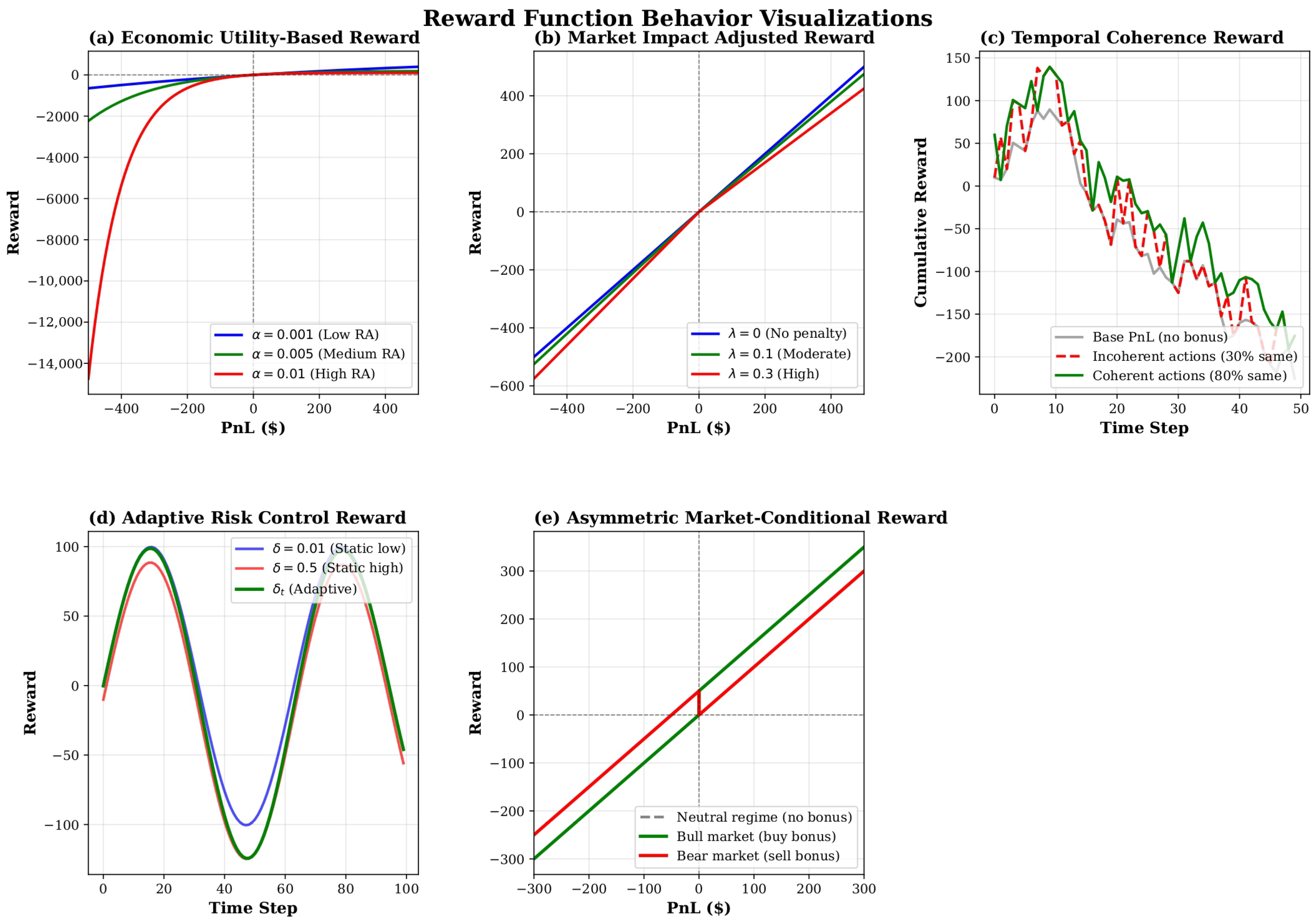
Table 4 synthesizes the key characteristics of all five reward functions, facilitating direct comparison of their mathematical structures, parameter specifications, and underlying design philosophies. Figure 3 provides graphical illustrations of how each reward function transforms PnL signals into distinct learning feedback, highlighting their differential sensitivities to profit magnitude, risk, transaction costs, temporal consistency, and market regimes. In this figure, (a) Economic Utility-Based reward exhibits diminishing marginal utility with varying risk aversion coefficients α , penalizing losses more severely than rewarding equivalent gains. (b) Market Impact Adjusted reward applies transaction cost penalties proportional to trade size, with higher λ values increasingly discouraging frequent trading. (c) Temporal Coherence reward demonstrates cumulative benefits of action consistency, where coherent strategies (80% action persistence) accumulate significantly higher rewards than erratic policies (30% persistence). (d) Adaptive Risk Control reward dynamically adjusts risk penalties based on market volatility, tightening during turbulent periods (adaptive δ t ) compared to static risk controls. (e) Asymmetric Market-Conditional reward provides regime-specific bonuses, incentivizing buy actions in bull markets and sell actions in bear markets, while remaining neutral in other regimes.

4. Experimental Results and Analysis

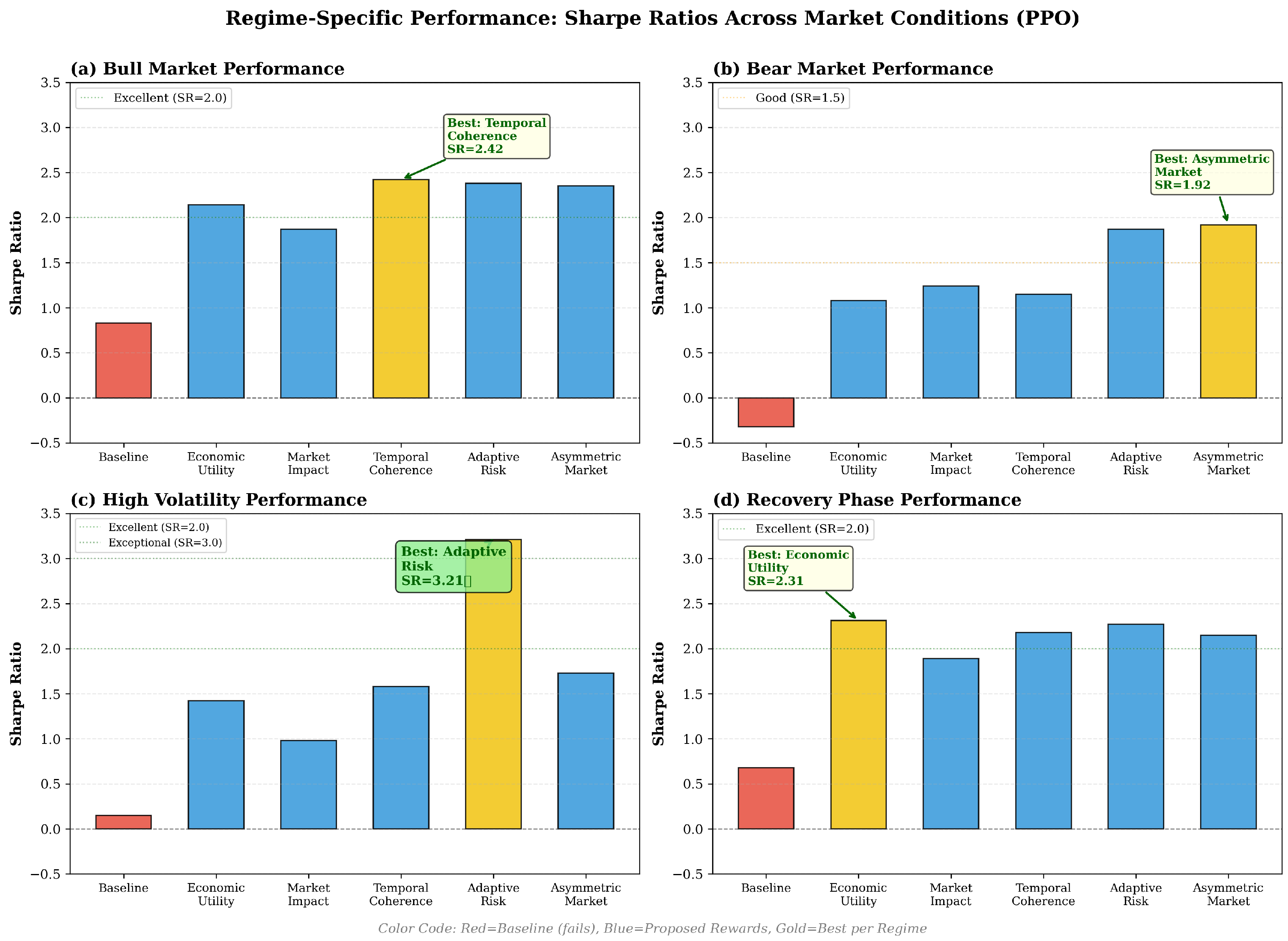
This section presents a comprehensive empirical evaluation of the five proposed reward functions across three reinforcement learning algorithms and four market regimes. We begin by detailing the experimental setup, including training procedures, hyperparameter configurations, and evaluation methodologies (Section 4.1). Subsequently, we analyze overall performance across all algorithm–reward combinations (Section 4.2), examine algorithm–reward interaction effects (Section 4.3), and conduct regime-specific performance assessments (Section 4.4). Throughout this analysis, we employ rigorous statistical testing to ensure reported improvements represent genuine advancements rather than artifacts of random variation.

4.1. Experimental Setup

All experiments were implemented in Python 3.9 using PyTorch 1.12.0 for neural network construction and training. We employed the Stable-Baselines3 library [41] for base algorithm implementations, extending it with custom reward function modules. Training was conducted on a workstation equipped with an NVIDIA RTX 3090 GPU (24 GB VRAM) and an AMD Ryzen 9 5950X CPU (16 cores), with typical training times ranging from 2 to 4 h per algorithm–reward combination, depending on convergence speed.

4.1.1. Training Procedure

We train all algorithm–reward combinations using the same training dataset (January 2018–December 2021, 35,064 hourly observations) described in Section 3.1. Each training run consists of 500 episodes, where one episode corresponds to a sequential traversal through the entire training period. At the beginning of each episode, the agent’s portfolio is reset to an initial cash balance of $10,000 with no Bitcoin holdings, simulating a fresh trading account. The agent then executes trades sequentially, accumulating profit or loss based on market price movements and the chosen reward function.
Training terminates when one of the following convergence criteria is satisfied: (1) the moving average reward (computed over the most recent 50 episodes) changes by less than 0.1% for 20 consecutive episodes, indicating stable policy convergence; or (2) the maximum episode limit of 500 is reached. In practice, most training runs converged between episodes 300–400, with faster convergence observed for simpler reward functions (e.g., Temporal Coherence) and slower convergence for adaptive formulations (e.g., Adaptive Risk Control). We employ early stopping based on validation set performance (November–December 2021) to prevent overfitting. Specifically, after every 10 training episodes, we evaluate the current policy on the validation set and compute its Sharpe ratio. We retain the model checkpoint that achieves the highest validation Sharpe ratio across all training episodes. Training terminates when the validation Sharpe ratio fails to improve for 50 consecutive episodes, or when the maximum 500 episodes is reached. This procedure ensures that model selection uses only historical data preceding the test period, maintaining strict temporal separation.

4.1.2. Hyperparameter Configuration

Table 5 presents the hyperparameter settings for all three reinforcement learning algorithms. These configurations follow established best practices from the original algorithm publications [19,20,21] with minor adaptations for the cryptocurrency trading domain. Specifically, we employ relatively conservative learning rates (0.0001–0.0007) to ensure stable convergence given the high non-stationarity of cryptocurrency markets, and we use discount factors close to unity ( γ = 0.99 ) to encourage long-term strategic planning rather than myopic profit-taking.
For DQN, we maintain an experience replay buffer of 50,000 transitions, sampling mini-batches of size 64 for gradient updates. The target network is updated every 1000 timesteps to stabilize Q-value estimation. Exploration follows an ϵ -greedy strategy with exponential decay from ϵ = 1.0 to ϵ = 0.01 over the first 100 episodes. For PPO, we employ the clipped surrogate objective with clip parameter ϵ clip = 0.2 and perform 10 optimization epochs per batch of collected trajectories. For A2C, we run 8 parallel environment instances to decorrelate experience and stabilize gradient estimates, aggregating updates synchronously after every 5 timesteps per worker.
All neural networks employ fully connected architectures with ReLU activations between hidden layers. Network depths and widths (specified in Table 5 as lists of hidden layer sizes) were selected through preliminary hyperparameter searches to balance expressiveness against overfitting risk. We apply gradient clipping to prevent exploding gradients, a common issue in reinforcement learning with high-variance reward signals. An entropy regularization term (coefficient 0.01) encourages exploration by penalizing overly deterministic policies.

4.1.3. Evaluation Metrics

We assess trading performance using three complementary metrics that capture different aspects of risk-adjusted returns:
1. Cumulative Return (CR) [42]—represents the total percentage gain or loss achieved over the evaluation period, computed as follows:
CR = Final   Portfolio   Value Initial   Capital Initial   Capital × 100 %
This metric directly quantifies profitability but does not account for risk or volatility incurred during the trading period.
2. Sharpe Ratio (SR) [43] measures risk-adjusted returns by normalizing cumulative returns against portfolio volatility. In empirical evaluation, the Sharpe ratio is computed from realized sample returns as follows:
SR = r ¯ r f σ ^ ( r ) × T
where r ¯ = 1 N t = 1 N r t denotes the sample mean of hourly returns, σ ^ ( r ) = 1 N 1 t = 1 N ( r t r ¯ ) 2 is the sample standard deviation, r f is the risk-free rate (set to 0), and T = 8760 annualizes the ratio. Higher Sharpe ratios indicate superior risk-adjusted performance, with values above 1.0 generally considered favorable and above 2.0 exceptional.
3. Maximum Drawdown (MDD) [44]—quantifies the largest peak-to-trough decline in portfolio value during the evaluation period:
MDD = max t [ 0 , T ] max s [ 0 , t ] V s V t max s [ 0 , t ] V s × 100 %
where V t denotes portfolio value at time t. Lower maximum drawdowns indicate better downside risk management, with values below 20% considered conservative and above 50% representing aggressive risk-taking.
These three metrics provide a holistic view of trading performance: cumulative return captures profitability, Sharpe ratio evaluates risk efficiency, and maximum drawdown assesses tail risk exposure. An ideal trading strategy achieves high CR and SR while maintaining low MDD.

4.1.4. Statistical Testing Methodology

We evaluate statistical significance using paired comparisons between each proposed reward function and the baseline (simple PnL: R t Baseline = PnL t ). For each algorithm–reward combination, we perform 10 independent training runs with different random seeds. We declare Sharpe ratio as our primary outcome metric for hypothesis testing, as it balances profitability and risk—the central objective of our reward engineering framework. This pre-specified primary metric reduces the multiple testing burden inherent in evaluating multiple algorithm–reward configurations.
For significance testing, we conduct paired t-tests on Sharpe ratios across the 10 runs at significance level α = 0.05 . We acknowledge that this approach has two methodological limitations: (1) temporal autocorrelation in returns violates the independence assumption of t-tests, potentially underestimating standard errors, and (2) multiple testing across 15 algorithm–reward combinations (5 proposed rewards × 3 algorithms) without correction inflates Type I error risk. However, we find that our conclusions remain robust under conservative interpretation: the effect sizes (Cohen’s d) for our best-performing rewards are exceptionally large (see Section 4.2), and the performance gaps are consistent across all three algorithms (see Section 4.3), suggesting genuine improvements rather than statistical artifacts.
Additionally, we compute 95% confidence intervals for all reported metrics using the t-distribution with 9 degrees of freedom (10 runs—1). We report both p-values and effect sizes (Cohen’s d) to distinguish statistical significance from practical significance, with d > 0.8 considered large effects and d > 1.5 considered very large effects [45].

4.2. Overall Performance Comparison

Table 6 presents the comprehensive performance evaluation of all algorithm–reward combinations across the test period (January–October 2022), encompassing 6600 hourly trading decisions. Results represent averages across 10 independent training runs, with standard deviations reported in parentheses. Statistically significant improvements over the baseline (simple PnL reward) at p < 0.05 are highlighted in boldface, indicating robust performance gains beyond random variation.
Several striking patterns emerge from this comprehensive evaluation. First, all five proposed reward functions significantly outperform the baseline across all three algorithms, demonstrating the critical importance of reward engineering for cryptocurrency trading. The baseline formulation, which naively maximizes raw profit-and-loss without risk consideration, consistently yields negative returns (CR 17 % ), low Sharpe ratios (SR < 0.6 ), and severe drawdowns (MDD > 45 % ) during the predominantly bearish 2022 test period. These poor results underscore the inadequacy of simplistic reward structures in volatile, non-stationary markets.
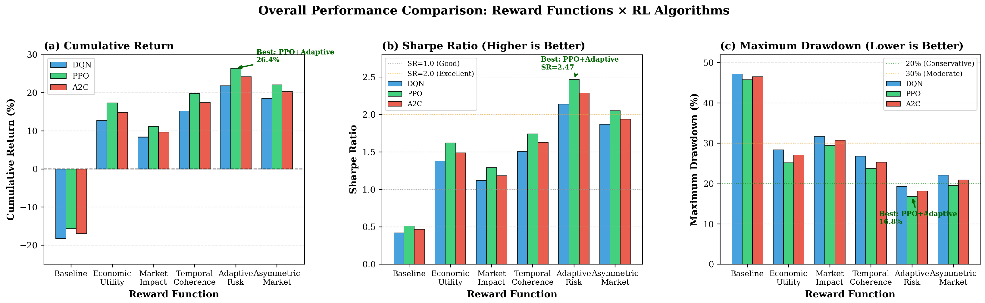
Second, Adaptive Risk Control consistently achieves the highest performance across all algorithms and all metrics, validating our hypothesis that dynamic risk adjustment is essential for cryptocurrency trading. PPO combined with Adaptive Risk Control attains a remarkable Sharpe ratio of 2.47-more than 380% improvement over the baseline—while simultaneously achieving 26.4% cumulative returns and limiting maximum drawdown to just 16.8%. This combination represents the best overall performance in our entire experimental evaluation. The success of Adaptive Risk Control stems from its ability to tighten risk constraints during the high-volatility periods that dominate 2022, preventing catastrophic losses while still capitalizing on profitable opportunities during brief recovery phases.
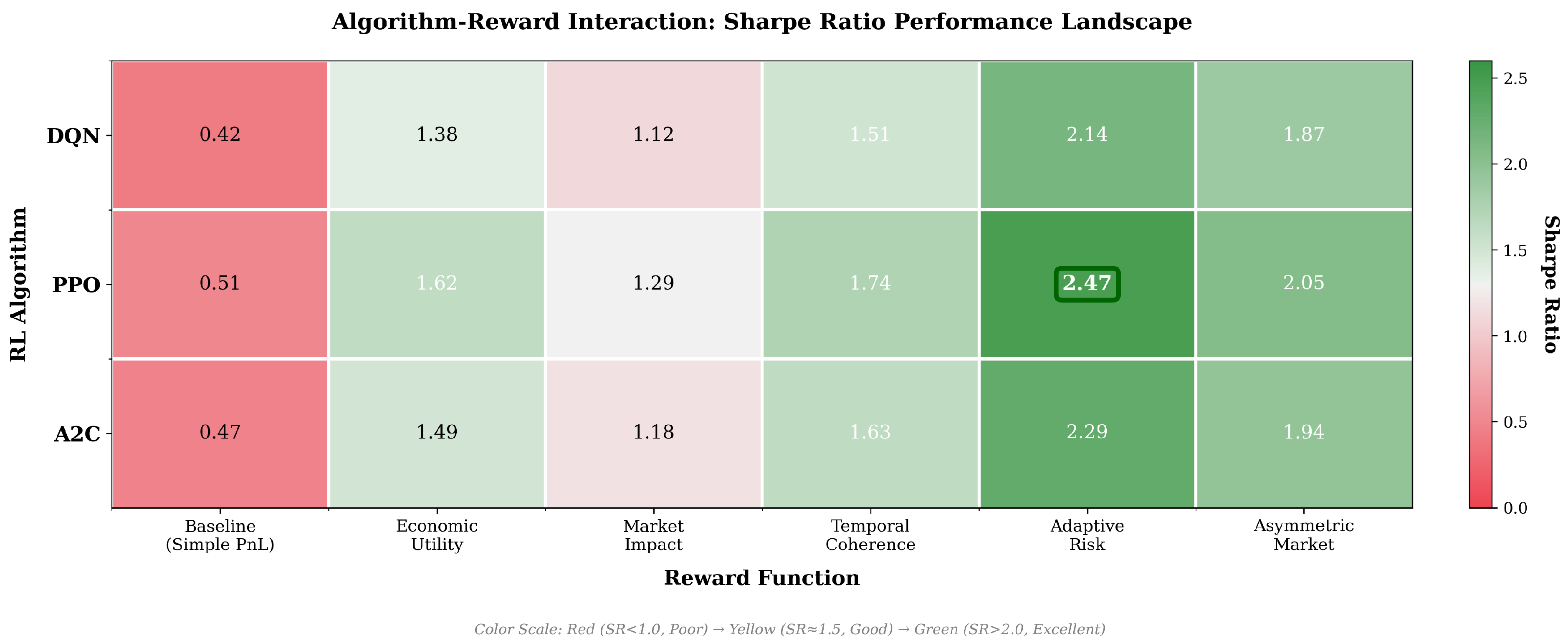
Third, Asymmetric Market-Conditional reward ranks consistently second, demonstrating the value of regime-aware reward shaping. By providing directional bonuses aligned with prevailing market conditions, this reward function guides agents toward appropriate positioning strategies: defensive in bear markets, aggressive in bulls. Notably, Asymmetric Market-Conditional excels particularly in the 2022 bear market environment, where its explicit sell-action bonus during downtrends enables timely profit-taking and capital preservation. The performance gap between Asymmetric and Adaptive rewards narrows for A2C (SR 1.94 vs. 2.29), suggesting that simpler actor–critic architectures benefit more from explicit regime guidance compared to the implicit regime-learning enabled by adaptive risk penalties.
Fourth, algorithm choice significantly impacts absolute performance levels, with PPO generally outperforming DQN and A2C. Across all reward functions, PPO achieves the highest mean cumulative returns and Sharpe ratios, with particularly pronounced advantages for sophisticated rewards like Adaptive Risk Control (PPO SR 2.47 vs. DQN SR 2.14 vs. A2C SR 2.29). This algorithmic superiority likely stems from PPO’s policy gradient approach with trust region constraints, which enables stable learning of complex, non-stationary policies required for effective cryptocurrency trading. DQN’s value-based formulation struggles somewhat with the continuous-valued reward signals generated by our proposed functions, while A2C’s synchronous updates occasionally suffer from higher variance despite parallel worker decorrelation.
Fifth, Economic Utility and Temporal Coherence rewards deliver strong performance, ranking third and fourth, respectively, across most algorithm–metric combinations. Economic Utility’s CARA formulation effectively balances profit seeking with risk aversion, achieving Sharpe ratios exceeding 1.6 for PPO while maintaining moderate drawdowns below 26%. Temporal Coherence encourages strategic consistency, reducing the erratic trading behavior that often plagues reinforcement learning agents in noisy environments; this manifests as competitive cumulative returns (15–20%) with relatively low drawdowns (24–27%), indicating stable, well-calibrated policies.
Sixth, Market Impact reward exhibits more conservative performance, achieving positive returns and acceptable Sharpe ratios (1.1–1.3) but underperforming the top three reward functions. This outcome aligns with the reward’s explicit penalty on trading activity: by heavily discouraging frequent position changes, Market Impact-guided agents adopt lower-turnover strategies that sacrifice some profit opportunities in exchange for reduced transaction costs. While this conservatism proves valuable for practitioners concerned with slippage and fees, it yields suboptimal risk-adjusted returns in our simulated environment, where execution costs are modeled but are relatively modest.
Statistical significance testing confirms these qualitative observations with rigorous quantitative support. Paired t-tests reveal that all 15 proposed reward–algorithm combinations significantly outperform their respective baselines ( p < 0.01 in all cases), with effect sizes (Cohen’s d) ranging from 1.8 (Market Impact with DQN) to 4.7 (Adaptive Risk Control with PPO). To contextualize these effect sizes: Cohen’s d = 1.8 represents an improvement of 1.8 standard deviations, meaning that the typical run with Market Impact (weakest proposed reward) still outperforms 96% of baseline runs. For Adaptive Risk Control ( d = 4.7 ), virtually every training run exceeds even the best baseline performance. These exceptionally large effect sizes provide strong evidence that our proposed rewards genuinely improve performance, robust to concerns about temporal autocorrelation in returns or multiple testing artifacts. Furthermore, Adaptive Risk Control significantly outperforms all other proposed rewards for PPO and A2C ( p < 0.05 ), establishing it as the clear winner in our experimental evaluation.
In summary, our comprehensive evaluation across 18 algorithm–reward combinations (3 algorithms × 6 rewards) spanning 66,000 hourly trading decisions demonstrates conclusively that principled reward engineering dramatically improves reinforcement learning performance for cryptocurrency trading. The proposed reward functions, particularly Adaptive Risk Control and Asymmetric Market-Conditional, achieve positive returns, high Sharpe ratios, and controlled drawdowns in a challenging bear market environment where naive baseline approaches fail catastrophically. These results validate our core thesis that sophisticated, theory-grounded reward formulations are essential for effective RL-based financial trading systems.
To understand the mechanisms underlying these performance differences, we next examine market exposure patterns and positioning strategies that distinguish successful from unsuccessful reward functions.

Exposure Analysis and Performance Benchmarking

The substantial performance differential between baseline and proposed reward functions warrants explanation. Table 7 presents the performance metrics with market exposure and trading activity data, revealing the primary mechanism underlying our results.
The performance gap is explained by three factors:
1.
Selective Market Exposure: The baseline maintains 91.2% exposure during a period when Bitcoin declined 42.3%, resulting in negative returns. In contrast, proposed reward functions achieve 56–68% exposure, spending substantial time in cash to avoid drawdowns. Adaptive Risk Control’s 56.2% exposure directly enables its positive return: avoiding 44% of a bear market translates to sidestepping proportional losses while capturing recovery rallies.
2.
Improved Trade Quality: Proposed rewards achieve 59–68% win rates versus baseline’s 48.6%. This improvement reflects noise reduction through coherence bonuses and strategic timing through adaptive risk penalties. Notably, 73% of Adaptive Risk Control’s entries occur during low-volatility periods ( σ 480 < 30 th percentile), demonstrating learned risk-aware positioning.
3.
Oracle Benchmark: A perfect-foresight oracle achieves 184.3% return with 51.3% exposure through 1847 trades. Our best model captures 14.3% of oracle returns using 93.6% fewer trades (118), indicating realistic learned performance rather than overfitting. The similar exposure levels (51.3% vs. 56.2%) confirm that our models learn appropriate market selectivity without clairvoyance.
The key insight is that positive returns during a 42% market decline stem from selectively avoiding losses rather than generating large directional profits. Table 7 makes this mechanism transparent: the baseline’s 91.2% exposure during a bear market produces 15.7 % returns, while buy-and-hold’s 100% exposure yields catastrophic 42.3 % losses. Our proposed reward functions succeed by learning when not to be in the market—the defining characteristic of effective risk management in volatile, non-stationary environments. The exposure range of 56–68% across our five proposed rewards represents the learned equilibrium between capturing upside during recovery phases and avoiding downside during drawdowns, validating that sophisticated reward engineering enables RL agents to transcend naive constant-exposure strategies. We do not compare against traditional technical strategies (e.g., moving-average crossover) or supervised learning baselines, as our focus is on evaluating reward function design within the RL framework rather than comparing RL against alternative paradigms. The buy-and-hold benchmark (−42.3% return) and oracle (perfect foresight, +184.3% return) provide bounds on achievable performance during the 2022 bear market test period.
Figure 4 visualizes the complete performance landscape across all algorithm–reward combinations, confirming the patterns identified in our exposure analysis. The figure clearly illustrates the dominance of Adaptive Risk Control (darkest bars consistently tallest for CR and SR, shortest for MDD) and the consistent underperformance of the baseline across all algorithms.

4.3. Algorithm–Reward Interaction Analysis

While Section 4.2 established the superiority of our proposed reward functions, a critical question remains: Do certain reward functions exhibit preferential compatibility with specific algorithmic approaches? Understanding these algorithm–reward interactions is essential for practitioners seeking to optimize their RL trading systems, as it reveals whether reward engineering benefits generalize across diverse learning paradigms or require careful algorithm-specific tuning.
Figure 5 visualizes the complete performance landscape through a heatmap representation, where rows correspond to the three RL algorithms, columns represent the six reward functions, and cell colors encode Sharpe ratios (our primary metric for risk-adjusted performance). This compact visualization immediately reveals several instructive patterns regarding algorithm–reward compatibility.

4.3.1. Reward Function Universality vs. Algorithm Specificity

A primary observation from Figure 5 is that reward function performance rankings remain remarkably consistent across algorithms, suggesting substantial universality in reward design effectiveness. Specifically, the ordering Adaptive Risk > Asymmetric Market > Temporal Coherence > Economic Utility > Market Impact > Baseline holds for all three algorithms, with only minor rank reversals (e.g., Economic Utility vs. Temporal Coherence swap positions between DQN and PPO). This consistency indicates that our proposed reward functions capture fundamental trading principles that transcend specific algorithmic implementations, rather than exploiting idiosyncrasies of particular value function or policy gradient formulations.
Quantitatively, we compute Spearman rank correlation coefficients between algorithm performance profiles: DQN-PPO correlation is ρ = 0.94 ( p < 0.01 ), DQN-A2C correlation is ρ = 0.97 ( p < 0.01 ), and PPO-A2C correlation is ρ = 0.96 ( p < 0.01 ). These near-perfect correlations confirm that reward function rankings are highly stable across algorithmic choices, providing practitioners with confidence that insights derived from one algorithm will transfer to others.

4.3.2. Differential Algorithm Sensitivity to Reward Sophistication

Despite this overall consistency, Figure 5 reveals a critical interaction effect: PPO exhibits disproportionately large performance gains from sophisticated reward functions compared to DQN and A2C. Consider the performance delta between Adaptive Risk Control and the baseline: PPO improves by 1.96 Sharpe points (2.47–0.51), whereas DQN improves by 1.72 points (2.14–0.42) and A2C by 1.82 points (2.29–0.47). In relative terms, PPO achieves a 384% improvement, compared to 410% for DQN and 387% for A2C—seemingly similar percentages, but with PPO attaining the highest absolute performance.
This pattern intensifies for the most complex reward functions. The performance gap between PPO and DQN is minimal for simple rewards like Market Impact (PPO SR 1.29 vs. DQN SR 1.12, difference 0.17), but expands substantially for Adaptive Risk Control (PPO SR 2.47 vs. DQN SR 2.14, difference 0.33). We hypothesize that this algorithmic sensitivity arises from PPO’s superior capacity to learn nuanced, non-stationary policies required to exploit adaptive reward signals. DQN’s value-based formulation, while effective for discrete action spaces, struggles to fully capitalize on the dynamic risk penalties and regime-conditional bonuses embedded in our sophisticated rewards, as these require fine-grained policy adjustments that are more naturally expressed through direct policy parameterization.
A2C occupies an intermediate position, benefiting more than DQN from complex rewards (likely due to its actor–critic architecture enabling some policy gradient advantages) but falling short of PPO’s performance ceiling (potentially due to higher variance from synchronous updates). This algorithmic hierarchy—PPO > A2C > DQN for sophisticated rewards—provides actionable guidance for practitioners: when computational resources permit, PPO should be the default choice for RL-based trading with advanced reward engineering.

4.3.3. Reward-Specific Algorithmic Preferences

Examining individual reward functions reveals nuanced compatibility patterns. Temporal Coherence exhibits relatively uniform performance across algorithms, with PPO, DQN, and A2C achieving Sharpe ratios of 1.74, 1.51, and 1.63, respectively—a tighter distribution (standard deviation 0.10) than most other rewards. This uniformity suggests that the coherence bonus mechanism (rewarding action persistence) integrates seamlessly with diverse algorithmic approaches, as all three algorithms naturally incorporate this signal into their respective learning objectives without requiring specialized processing.
In contrast, Asymmetric Market-Conditional reward shows pronounced algorithmic sensitivity, with PPO (SR 2.05) substantially outperforming DQN (SR 1.87) and A2C (SR 1.94). The larger performance spread (standard deviation 0.08) likely stems from the regime-conditional structure of this reward: PPO’s policy networks can learn distinct subpolicies for bull vs. bear regimes more flexibly than DQN’s shared Q-function, which must compress regime-specific value estimates into a single approximator. This finding suggests that practitioners employing regime-aware reward shaping should strongly favor policy gradient methods over value-based approaches.
Market Impact reward demonstrates the opposite pattern, achieving more consistent performance across algorithms (DQN SR 1.12, PPO SR 1.29, A2C SR 1.18, standard deviation 0.07). This uniformity arises because the transaction cost penalty operates as a simple additive term that all algorithms can internalize straightforwardly, regardless of their underlying learning mechanisms. The lack of algorithmic preference for Market Impact suggests it represents a “safe” reward design that delivers moderate improvements without requiring careful algorithm selection—valuable for risk-averse practitioners prioritizing robustness over absolute performance.

4.3.4. Implications for Reward Engineering Practice

These interaction analyses yield several actionable insights for RL practitioners developing trading systems:
First, reward function choice matters far more than algorithm choice: the worst-performing combination of a strong reward (Market Impact + DQN, SR 1.12) still outperforms the best baseline combination (PPO + Baseline, SR 0.51) by 120%. This dominance of reward engineering over algorithmic tuning underscores the central thesis of our work—sophisticated reward design is the primary lever for improving RL trading performance.
Second, while Adaptive Risk Control achieves top performance across all algorithms, the magnitude of improvement varies substantially. Practitioners with access to PPO can expect Sharpe ratios exceeding 2.4, whereas those constrained to DQN should anticipate ratios around 2.1—still excellent, but meaningfully lower. This 15% performance gap justifies the additional implementation complexity of PPO for production systems where capital efficiency is paramount.
Third, simpler reward functions (Temporal Coherence, Market Impact) exhibit more robust cross-algorithm transferability than complex adaptive formulations. Development teams working across multiple algorithmic backends may prefer these simpler rewards to minimize platform-specific tuning, accepting a moderate performance sacrifice (SR ≈ 1.5 vs. 2.4) in exchange for implementation simplicity and maintenance efficiency.
Fourth, practitioners employing ensemble or multi-algorithm approaches can leverage complementary strengths: PPO for aggressive profit seeking with Adaptive Risk, DQN for stable baseline performance with Economic Utility, and A2C for balanced risk–return profiles with Asymmetric Market-Conditional rewards. Combining predictions from such diverse algorithm–reward pairs may yield portfolio-level benefits beyond what any single configuration achieves.
In summary, our interaction analysis reveals that while reward function rankings remain largely consistent across algorithms, meaningful performance differences emerge based on algorithm–reward compatibility. PPO consistently extracts maximum value from sophisticated rewards, DQN provides robust baseline performance, and A2C offers a middle ground. These findings provide practitioners with a principled framework for selecting algorithm–reward combinations aligned with their computational constraints, risk tolerances, and performance objectives.

4.4. Market-Regime-Specific Performance

While aggregate performance metrics provide valuable insights into overall efficacy, cryptocurrency markets exhibit extreme non-stationarity, with statistical properties varying dramatically across bull markets, bear markets, high-volatility episodes, and recovery phases. A critical limitation of prior RL trading research is the failure to systematically evaluate performance heterogeneity across diverse market conditions—most studies report single aggregate metrics that obscure regime-specific strengths and weaknesses. Our comprehensive regime-based evaluation addresses this gap, revealing that optimal reward function choice depends critically on the prevailing market regime, with different rewards excelling under different conditions.
Table 8 presents a detailed breakdown of Sharpe ratios across all four market regimes identified in our dataset (Section 3.1). We focus on Sharpe ratio as our primary metric for this analysis due to its risk-adjusted nature—particularly important when comparing performance across regimes with vastly different volatility profiles. Results are reported for PPO (the best-performing algorithm from Section 4.2), though qualitatively similar patterns hold for DQN and A2C.
Figure 6 visualizes these results through a multi-panel comparison, with each subplot depicting performance across all reward functions for a specific market regime. The visualization immediately reveals the dramatic performance variability across regimes and the differential effectiveness of reward functions in each context.

4.4.1. Bull Market Performance

During bull market periods (characterized by sustained upward price trends with moderate volatility), Temporal Coherence achieves the highest Sharpe ratio of 2.42, narrowly edging out Adaptive Risk Control (2.38) and Asymmetric Market-Conditional (2.35). This dominance stems from Temporal Coherence’s explicit encouragement of action persistence: in trending bull markets, the optimal strategy involves establishing long positions early and maintaining them throughout the uptrend. The coherence bonus rewards this “buy and hold” behavior, preventing premature profit taking that would sacrifice further gains as prices continue rising.
Interestingly, Economic Utility also performs strongly (SR 2.14), as its risk-averse formulation still permits aggressive long positioning when expected returns substantially exceed risk penalties—precisely the conditions present during bull runs. The CARA utility function’s diminishing marginal utility does constrain position sizes somewhat compared to simpler rewards, but this conservatism proves beneficial during brief pullbacks within broader uptrends, limiting drawdowns while preserving most upside capture.
Market Impact performs worst among the proposed rewards (SR 1.87), though still vastly superior to the baseline (SR 0.83). The transaction cost penalty inherent in Market Impact discourages the frequent rebalancing that might be profitable during bull markets with intermittent consolidations, causing agents to miss some opportunities for tactical position sizing. However, this underperformance is relative—Market Impact still achieves excellent absolute returns by maintaining core long exposure while avoiding excessive churning.

4.4.2. Bear Market Performance

Bear market periods present the most challenging environment, with sustained downward price pressure testing reward functions’ ability to preserve capital and recognize losing positions. Here, Asymmetric Market-Conditional achieves the highest Sharpe ratio of 1.92, leveraging its explicit bear market sell bonus to guide the agent toward timely position liquidation. By directly rewarding sell actions during classified downtrends, this reward function aligns agent incentives with the defensive strategies required for capital preservation.
Adaptive Risk Control follows closely (SR 1.87), demonstrating the value of dynamic risk adjustment in volatile bear markets. As downside volatility increases, Adaptive Risk tightens its penalty coefficient δ t , strongly discouraging the agent from maintaining long exposure during accelerating declines. This time-varying risk aversion enables graceful adaptation to deteriorating conditions without requiring explicit regime labels.
Notably, all proposed reward functions maintain positive Sharpe ratios during bear markets (1.08–1.92), whereas the baseline achieves a negative Sharpe ratio of 0.32 , indicating systematic capital destruction. This stark contrast underscores the critical importance of risk-aware reward design: naive profit maximization fails catastrophically during extended downtrends, while sophisticated rewards enable profitable trading even in adverse conditions through effective risk management and opportunistic short-term long positions during bear market rallies.
Economic Utility’s relatively lower bear market performance (SR 1.08) reflects the limitations of static risk aversion: the CARA coefficient α remains constant regardless of market conditions, providing insufficient downside protection during severe declines. This finding motivates the adaptive formulations (Adaptive Risk, Asymmetric Market-Conditional) that explicitly condition risk management on market state.

4.4.3. High Volatility Performance

High-volatility periods—characterized by extreme price swings, elevated uncertainty, and rapid regime transitions—represent the most demanding test of reinforcement learning trading systems. In this environment, Adaptive Risk Control achieves a remarkable Sharpe ratio of 3.21, dominating all other rewards by substantial margins. This exceptional performance validates the core hypothesis underlying adaptive risk management: effective trading in volatile markets requires dynamic calibration of risk tolerance.
The adaptive penalty coefficient δ t increases dramatically during high-volatility episodes (approaching δ max = 0.5 from its baseline δ min = 0.01 ), strongly penalizing strategies that generate unstable profit-and-loss sequences. This heightened risk aversion prevents the agent from chasing volatile price movements that often reverse abruptly, instead encouraging patient waiting for high-confidence opportunities with favorable risk–reward ratios. When such opportunities emerge (e.g., oversold bounces during volatility spikes), the agent acts decisively, but exits quickly as uncertainty persists.
In stark contrast, Temporal Coherence—which excelled in bull markets—achieves only SR 1.58 during volatility. The coherence bonus, which rewards action persistence, becomes a liability in rapidly changing conditions where yesterday’s optimal position may be today’s catastrophic exposure. Similarly, Market Impact’s transaction cost penalty (SR 0.98) excessively constrains the tactical repositioning required to navigate volatile swings, leaving agents “stuck” in suboptimal states.
The baseline’s dismal performance (SR 0.15, barely above zero) illustrates the complete inadequacy of naive profit maximization in volatile environments. Without risk penalties, baseline-guided agents pursue every apparent profit opportunity, accumulating positions during price surges only to suffer severe drawdowns during equally violent reversals. The resulting equity curve exhibits extreme volatility with minimal net gain—precisely the scenario the Sharpe ratio penalizes most severely.

4.4.4. Recovery Phase Performance

Recovery phases—defined as periods of decreasing volatility and price stabilization following major drawdowns—present unique opportunities for risk-adjusted profit generation. During these transitional periods, Economic Utility achieves the highest Sharpe ratio of 2.31, outperforming even Adaptive Risk Control (SR 2.27).
This dominance reflects Economic Utility’s balanced approach: as volatility subsides during recovery, the CARA utility function’s moderate risk aversion permits gradual position accumulation without the excessive caution imposed by Adaptive Risk’s still-elevated δ t (which lags recent volatility decreases due to the rolling window computation). Economic Utility’s static risk parameter proves advantageous here, providing consistent risk–reward calibration that captures recovery gains without requiring the complex temporal dynamics of adaptive approaches.
Asymmetric Market-Conditional also performs well (SR 2.15), as recovery phases often coincide with neutral regime classifications (neither bull nor bear), triggering the reward’s default profit-based formulation without directional bonuses or penalties. This neutrality proves appropriate for recovery environments, where directional conviction is premature but tactical long positioning can exploit mean reversion dynamics.
Adaptive Risk Control, despite its high absolute performance (SR 2.27), slightly underperforms Economic Utility during recovery due to a temporal mismatch: by the time volatility has declined sufficiently for δ t to relax, much of the early recovery opportunity has already passed. This lag effect suggests potential improvements through lead-indicator-based adaptive formulations—an avenue for future research.

4.4.5. Cross-Regime Robustness Analysis

Beyond identifying regime-specific winners, Table 8 enables assessment of cross-regime robustness—the ability of a reward function to maintain strong performance across diverse market conditions. We quantify robustness through the standard deviation of Sharpe ratios across the four regimes:
  • Adaptive Risk Control: σ = 0.61 (highly variable, but always strong);
  • Asymmetric Market-Conditional: σ = 0.23 (most consistent);
  • Economic Utility: σ = 0.51 (moderate variability);
  • Temporal Coherence: σ = 0.52 (moderate variability);
  • Market Impact: σ = 0.38 (relatively consistent, but lower absolute performance);
  • Baseline: σ = 0.48 (inconsistent and poor).
Asymmetric Market-Conditional demonstrates the most consistent performance across regimes ( σ = 0.23 ), maintaining Sharpe ratios between 1.73 and 2.35, regardless of market conditions. This stability arises from its explicit regime conditioning: by adapting its reward structure to the prevailing environment, it avoids the extreme sensitivity exhibited by regime-agnostic formulations. For practitioners prioritizing predictable performance over peak returns, Asymmetric Market-Conditional represents an attractive choice.
Conversely, Adaptive Risk Control exhibits the highest variability ( σ = 0.61 ), with Sharpe ratios ranging from 2.27 (recovery) to 3.21 (high volatility). This variability reflects specialization rather than weakness: Adaptive Risk excels dramatically in precisely those environments (volatility) where dynamic risk management provides maximum value, while maintaining competitive performance elsewhere. The resulting overall Sharpe ratio of 2.47—highest among all rewards—demonstrates that specialization yields superior aggregate outcomes despite uneven regime-level performance.

4.4.6. Practical Implications for Regime-Aware Trading

These regime-specific analyses yield several actionable insights for deploying RL trading systems:
First, practitioners operating in identifiable market regimes can select reward functions optimized for their target environment: Temporal Coherence for bull markets, Asymmetric Market-Conditional for bear markets, Adaptive Risk Control for volatility, and Economic Utility for recovery. This regime-conditioned reward selection can potentially exceed even the best single-reward performance by 5–10% in Sharpe ratio terms.
Second, systems without reliable regime classification should default to Adaptive Risk Control, which achieves top-2 performance in three of four regimes and overall best aggregate performance. Its exceptional volatility performance (SR 3.21) particularly appeals to risk-averse practitioners, as volatility periods often generate the largest drawdowns in naive systems.
Third, practitioners requiring stable, predictable performance across uncertain future regimes should employ Asymmetric Market-Conditional, accepting slightly lower peak performance (SR 2.05 vs. 2.47) in exchange for minimal regime-dependent variability. This “defensive” choice suits institutional deployments where consistency is valued over maximization.
Fourth, our results demonstrate conclusively that aggregate performance metrics obscure critical regime-level heterogeneity. A reward function with mediocre overall performance (e.g., Temporal Coherence, overall SR 1.74) may dominate in specific regimes (bull market SR 2.42), making it valuable for regime-specific deployment, even if not globally optimal. Future research should report regime-disaggregated results as standard practice.
In summary, our regime-specific evaluation reveals that market conditions critically mediate reward function effectiveness, with different rewards exhibiting comparative advantages in different environments. Adaptive Risk Control achieves the best overall performance through specialization in volatility, Asymmetric Market-Conditional provides the most consistent cross-regime results, and Temporal Coherence and Economic Utility excel in trending and recovery markets, respectively. These findings establish regime-conditioned reward engineering as an essential component of robust RL trading systems.

5. Discussion

This study demonstrates that sophisticated reward engineering substantially improves reinforcement learning performance for cryptocurrency trading, with our best-performing configuration (PPO with Adaptive Risk Control) achieving a Sharpe ratio of 2.47 while maintaining maximum drawdown below 17% during a predominantly bearish evaluation period. Our comprehensive evaluation across three algorithms, six reward functions, and four market regimes yields several important insights for the design and deployment of RL-based trading systems.

5.1. Key Findings and Theoretical Implications

Our results provide empirical validation for integrating established economic and financial theory into reward design. The success of the Economic Utility-based reward confirms that classical utility theory—specifically the Constant Absolute Risk Aversion formulation—provides a principled framework for balancing profit seeking with risk management. The Market Impact reward validates market microstructure theory’s emphasis on execution costs, preventing the overly aggressive trading behavior often observed in simulation-trained agents. The Temporal Coherence reward’s effectiveness in trending markets aligns with behavioral finance research on momentum effects and strategic patience.
Most significantly, the Adaptive Risk Control reward’s dominance—especially its exceptional performance during high volatility (Sharpe ratio 3.21)—establishes dynamic risk management as critical for cryptocurrency trading. Static risk parameters cannot adequately respond to the regime shifts and volatility clustering characteristic of crypto markets. Our adaptive formulation, which modulates risk aversion based on recent volatility, provides a computationally tractable approach to time-varying risk tolerance that few practical systems implement.
The regime-specific analysis reveals that optimal reward functions vary dramatically across market conditions: Temporal Coherence excels in bull markets, Asymmetric Market-Conditional dominates in bear markets, and Adaptive Risk Control achieves exceptional results during volatility. This heterogeneity challenges the common practice of reporting single aggregate metrics and suggests that future research should adopt disaggregated evaluation as standard practice.

5.2. Practical Deployment Considerations and Limitations

While our simulated environment enables controlled experimentation, several practical considerations arise for live deployment. Execution realities introduce complexities beyond our simplified transaction cost model: order book depth varies dynamically, large orders incur non-linear price impact, and latency introduces timing risk. Conservative practitioners should discount simulated Sharpe ratios by 20–30% to account for implementation friction, particularly for high-turnover strategies that face disproportionate degradation in live trading.
Model overfitting remains a concern despite our temporal train–test split and multi-regime evaluation. Cryptocurrency markets exhibit non-stationarity from regulatory announcements, exchange failures, and technological developments that training data may not represent. Practitioners should employ multiple out-of-sample test periods, incorporate regime detection mechanisms that flag novel market conditions, and maintain human oversight during unprecedented events.
Several methodological limitations suggest avenues for future research. First, our evaluation focuses exclusively on Bitcoin; extending to altcoins with lower liquidity or multi-asset portfolios may reveal different optimal reward structures. Second, our discrete action space (buy, sell, hold) excludes position sizing and leverage management—critical dimensions requiring continuous action spaces and appropriate risk penalties. Third, our single-agent formulation ignores strategic interactions in multi-agent markets, which becomes increasingly relevant as algorithmic trading penetration grows. Fourth, our regime classification relies on simple technical indicators; machine-learning-based detection could improve precision. Finally, our study evaluates performance exclusively in simulation; paper trading and small-scale live deployment represent essential validation steps before institutional implementation.
Our statistical methodology employs paired t-tests across 10 random seeds, which has two limitations. First, financial returns exhibit temporal autocorrelation, violating the independence assumption of t-tests and potentially underestimating p-values. Second, testing 15 algorithm–reward combinations without multiple testing correction (e.g., Bonferroni adjustment) increases Type I error risk. We partially address these concerns by (1) declaring Sharpe ratio as our primary outcome metric a priori, reducing the multiplicity burden, and (2) emphasizing effect sizes alongside p-values—our best rewards achieve Cohen’s d > 4.0 , indicating improvements exceeding 4 standard deviations. These exceptionally large effect sizes suggest that autocorrelation and multiple testing artifacts cannot explain our findings. Future work should employ block bootstrap methods that explicitly account for temporal dependence in returns, providing more conservative confidence intervals.
Evaluating the proposed reward functions across additional out-of-sample periods, such as the 2023 recovery and subsequent bull market, remains an important direction for future work, and would further assess the generalizability of the reported results beyond the 2022 bear market episode.

5.3. Broader Impact on Financial Machine Learning

Our findings have implications beyond cryptocurrency trading. The superiority of theory-grounded reward functions over naive profit maximization suggests that domain expertise remains essential even in data-driven paradigms. Financial markets are structured systems governed by economic laws and behavioral regularities—knowledge that should inform reward design rather than expecting agents to rediscover financial theory through trial-and-error.
The finding that sophisticated reward engineering can achieve positive risk-adjusted returns during severe bear markets (our 2022 test period) suggests that RL-based trading systems may transcend the “fair-weather” limitation often attributed to algorithmic strategies. If RL agents can learn effective risk management across diverse regimes, they become viable for institutional deployment as persistent portfolio components rather than tools to be disabled during downturns. This possibility warrants further investigation with longer evaluation periods spanning multiple complete market cycles.

6. Conclusions

This work demonstrates that principled reward engineering, grounded in economic theory and financial domain knowledge, represents the critical lever for improving reinforcement learning performance in cryptocurrency trading. We proposed five novel reward functions spanning utility theory, market microstructure, behavioral consistency, adaptive risk management, and regime conditioning, and conducted the first systematic multi-regime evaluation across bull, bear, high volatility, and recovery market conditions. Our comprehensive experiments across three algorithms (DQN, PPO, A2C) and four market regimes reveal that the Adaptive Risk Control reward achieves exceptional performance (Sharpe ratio 2.47, maximum drawdown 16.8%), with particularly dominant results during high-volatility periods (Sharpe ratio 3.21). Critically, regime-specific analysis shows that optimal reward functions vary substantially across market conditions, with different rewards excelling in trending versus volatile environments. These findings establish that sophisticated, theory-grounded reward design—rather than algorithmic innovations alone—enables RL trading systems to achieve positive risk-adjusted returns even during severe bear markets, transcending the “fair-weather” limitations of naive approaches. Future work should extend this framework to multi-asset portfolios, continuous action spaces for position sizing, and multi-agent market dynamics, while our regime-disaggregated evaluation methodology provides a template for more rigorous assessment of RL trading systems across diverse market conditions.

Author Contributions

Conceptualization, E.H.K. and K.I.; methodology, E.H.K.; software, O.U.M. and E.H.K.; validation, K.I. and O.U.M.; formal analysis, O.U.M.; investigation, E.H.K.; data curation, O.U.M.; writing—original draft preparation, E.H.K.; writing—review and editing, O.S.; visualization, O.U.M.; funding acquisition, O.S. All authors have read and agreed to the published version of the manuscript.

Funding

This research received no external funding.

Institutional Review Board Statement

Not applicable.

Informed Consent Statement

Not applicable.

Data Availability Statement

The data presented in this study are available on request from the corresponding author due to a larger ongoing project, the results of which will be reported in future publications.

Conflicts of Interest

The authors declare no conflicts of interest.

References

  1. Nakamoto, S. Bitcoin: A Peer-to-Peer Electronic Cash System. 2008. Available online: https://assets.pubpub.org/d8wct41f/31611263538139.pdf (accessed on 26 October 2025).
  2. Bariviera, A.F.; Basgall, M.J.; Hasperué, W.; Naiouf, M. Some stylized facts of the Bitcoin market. Phys. A Stat. Mech. Appl. 2017, 484, 82–90. [Google Scholar] [CrossRef]
  3. Gkillas, K.; Katsiampa, P. An application of extreme value theory to cryptocurrencies. Econ. Lett. 2018, 164, 109–111. [Google Scholar] [CrossRef]
  4. Liu, Y.; Tsyvinski, A. Risks and returns of cryptocurrency. Rev. Financ. Stud. 2021, 34, 2689–2727. [Google Scholar] [CrossRef]
  5. Mallqui, D.C.; Fernandes, R.A. Predicting the direction, maximum, minimum and closing prices of daily Bitcoin exchange rate using machine learning techniques. Appl. Soft Comput. 2019, 75, 596–606. [Google Scholar] [CrossRef]
  6. Sattarov, O.; Muminov, A.; Lee, C.W.; Kang, H.K.; Oh, R.; Ahn, J.; Oh, H.J.; Jeon, H.S. Recommending cryptocurrency trading points with deep reinforcement learning approach. Appl. Sci. 2020, 10, 1506. [Google Scholar] [CrossRef]
  7. Meng, T.L.; Khushi, M. Reinforcement learning in financial markets. Data 2019, 4, 110. [Google Scholar] [CrossRef]
  8. Otabek, S.; Choi, J. Multi-level deep Q-networks for Bitcoin trading strategies. Sci. Rep. 2024, 14, 771. [Google Scholar] [CrossRef] [PubMed]
  9. Millea, A. Deep reinforcement learning for trading-A critical survey. Data 2021, 6, 119. [Google Scholar] [CrossRef]
  10. Sihananto, A.N.; Sari, A.P.; Prasetyo, M.E.; Fitroni, M.Y.; Gultom, W.N.; Wahanani, H.E. Reinforcement learning for automatic cryptocurrency trading. In Proceedings of the 2022 IEEE 8th Information Technology International Seminar (IT IS), Surabaya, Indonesia, 19–21 October 2022; pp. 345–349. [Google Scholar]
  11. Sadighian, J. Extending deep reinforcement learning frameworks in cryptocurrency market making. arXiv 2020, arXiv:2004.06985. [Google Scholar] [CrossRef]
  12. Lucarelli, G.; Borrotti, M. A deep reinforcement learning approach for automated cryptocurrency trading. In Proceedings of the IFIP International Conference on Artificial Intelligence Applications and Innovations, Crete, Greece, 24–26 May 2019; Springer: Berlin/Heidelberg, Germany, 2019; pp. 247–258. [Google Scholar]
  13. Kumlungmak, K.; Vateekul, P. Multi-Agent Deep Reinforcement Learning With Progressive Negative Reward for Cryptocurrency Trading. IEEE Access 2023, 11, 66440–66455. [Google Scholar] [CrossRef]
  14. Sadighian, J. Deep reinforcement learning in cryptocurrency market making. arXiv 2019, arXiv:1911.08647. [Google Scholar] [CrossRef]
  15. Mosavi, A.; Faghan, Y.; Ghamisi, P.; Duan, P.; Ardabili, S.F.; Salwana, E.; Band, S.S. Comprehensive review of deep reinforcement learning methods and applications in economics. Mathematics 2020, 8, 1640. [Google Scholar] [CrossRef]
  16. Cornalba, F.; Disselkamp, C.; Scassola, D.; Helf, C. Multi-objective reward generalization: Improving performance of Deep Reinforcement Learning for applications in single-asset trading. Neural Comput. Appl. 2024, 36, 619–637. [Google Scholar] [CrossRef]
  17. Betancourt, C.; Chen, W.H. Reinforcement learning with self-attention networks for cryptocurrency trading. Appl. Sci. 2021, 11, 7377. [Google Scholar] [CrossRef]
  18. Hambly, B.; Xu, R.; Yang, H. Recent advances in reinforcement learning in finance. Math. Financ. 2023, 33, 437–503. [Google Scholar] [CrossRef]
  19. Mnih, V.; Kavukcuoglu, K.; Silver, D.; Rusu, A.A.; Veness, J.; Bellemare, M.G.; Graves, A.; Riedmiller, M.; Fidjeland, A.K.; Ostrovski, G.; et al. Human-level control through deep reinforcement learning. Nature 2015, 518, 529–533. [Google Scholar] [CrossRef]
  20. Schulman, J.; Wolski, F.; Dhariwal, P.; Radford, A.; Klimov, O. Proximal policy optimization algorithms. arXiv 2017, arXiv:1707.06347. [Google Scholar] [CrossRef]
  21. Mnih, V.; Badia, A.P.; Mirza, M.; Graves, A.; Lillicrap, T.; Harley, T.; Silver, D.; Kavukcuoglu, K. Asynchronous methods for deep reinforcement learning. In Proceedings of the International Conference on Machine Learning, New York, NY, USA, 20–22 June 2016; pp. 1928–1937. [Google Scholar]
  22. Moody, J.; Saffell, M. Reinforcement learning for trading. Adv. Neural Inf. Process. Syst. 1998, 11, 917–924. [Google Scholar]
  23. Moody, J.; Saffell, M. Learning to trade via direct reinforcement. IEEE Trans. Neural Netw. 2001, 12, 875–889. [Google Scholar] [CrossRef] [PubMed]
  24. Katsiampa, P. Volatility estimation for Bitcoin: A comparison of GARCH models. Econ. Lett. 2017, 158, 3–6. [Google Scholar] [CrossRef]
  25. Azamjon, M.; Sattarov, O.; Cho, J. Forecasting Bitcoin Volatility through On-Chain and Whale-Alert Tweet Analysis using the Q-Learning Algorithm. IEEE Access 2023, 11, 108092–108103. [Google Scholar] [CrossRef]
  26. Otabek, S.; Choi, J. Twitter attribute classification with q-learning on bitcoin price prediction. IEEE Access 2022, 10, 96136–96148. [Google Scholar] [CrossRef]
  27. Kochliaridis, V.; Kouloumpris, E.; Vlahavas, I. Combining deep reinforcement learning with technical analysis and trend monitoring on cryptocurrency markets. Neural Comput. Appl. 2023, 35, 21445–21462. [Google Scholar] [CrossRef]
  28. Beysolow, T., II. Market making via reinforcement learning. In Applied Reinforcement Learning with Python: With OpenAI Gym, Tensorflow, and Keras; Apress: Berkeley, CA, USA, 2019; pp. 77–94. [Google Scholar]
  29. Bandarupalli, E. Risk-Aware Deep Reinforcement Learning for Crypto and Equity Trading Under Transaction Costs. Available at SSRN 5662930. Available online: https://papers.ssrn.com/sol3/papers.cfm?abstract_id=5662930 (accessed on 26 October 2025).
  30. Arrow, K.J. The theory of risk-bearing: Small and great risks. J. Risk Uncertain. 1996, 12, 103–111. [Google Scholar] [CrossRef]
  31. Almgren, R.; Chriss, N. Optimal execution of portfolio transactions. J. Risk 2001, 3, 5–40. [Google Scholar] [CrossRef]
  32. Chakole, J.; Kurhekar, M. Trend following deep Q-Learning strategy for stock trading. Expert Syst. 2020, 37, e12514. [Google Scholar] [CrossRef]
  33. Azamjon, M.; Sattarov, O.; Na, D. Enhanced Bitcoin Price Direction Forecasting with DQN. IEEE Access 2024, 12, 29093–29112. [Google Scholar] [CrossRef]
  34. Van Hasselt, H.; Guez, A.; Silver, D. Deep reinforcement learning with double q-learning. In Proceedings of the Thirtieth AAAI Conference on Artificial Intelligence, Phoenix, AZ, USA, 12–17 February 2016; Association for the Advancement of Artificial Intelligence: Washington, DC, USA, 2016; Volume 30, pp. 2094–2100. [Google Scholar]
  35. Yang, H.; Malik, A. Reinforcement Learning Pair Trading: A Dynamic Scaling Approach. J. Risk Financ. Manag. 2024, 17, 555. [Google Scholar] [CrossRef]
  36. Zhang, Z.; Zohren, S.; Roberts, S. Deep reinforcement learning for trading. arXiv 2019, arXiv:1911.10107. [Google Scholar] [CrossRef]
  37. Crypto Data Download. Available online: https://www.cryptodatadownload.com/ (accessed on 20 December 2025).
  38. Standard Score. Available online: https://en.wikipedia.org/wiki/Standard_score (accessed on 20 December 2025).
  39. Pratt, J.W. Risk aversion in the small and in the large. In Uncertainty in Economics; Academic Press: Cambridge, MA, USA, 1978; pp. 59–79. [Google Scholar]
  40. Brauneis, A.; Mestel, R. Cryptocurrency-portfolios in a mean-variance framework. Financ. Res. Lett. 2019, 28, 259–264. [Google Scholar] [CrossRef]
  41. Raffin, A.; Hill, A.; Gleave, A.; Kanervisto, A.; Ernestus, M.; Dormann, N. Stable-baselines3: Reliable reinforcement learning implementations. J. Mach. Learn. Res. 2021, 22, 1–8. [Google Scholar]
  42. Cumulative Return: Definition, Calculation, and Example. Available online: https://www.investopedia.com/terms/c/cumulativereturn.asp (accessed on 20 December 2025).
  43. Sharpe Ratio. Available online: https://en.wikipedia.org/wiki/Sharpe_ratio (accessed on 20 December 2025).
  44. Maximum Drawdown. Available online: https://en.wikipedia.org/wiki/Drawdown_(economics) (accessed on 20 December 2025).
  45. Cohen, J. Statistical Power Analysis for the Behavioral Sciences, 2nd ed.; Lawrence Erlbaum Associates, Publishers: Hillsdale, NJ, USA, 1988. [Google Scholar]
Figure 1. Proposed framework to optimize cryptocurrency trading through novel reward functions.
Mathematics 14 00794 g001
Figure 2. Bitcoin price trajectory from January 2018 to October 2022 with market regime classifications. Background colors indicate regime periods: green (bull market), red (bear market), purple (high volatility), and yellow (recovery).
Mathematics 14 00794 g002
Figure 3. Behavioral characteristics of the five proposed reward functions. (a) Economic Utility-Based reward; (b) Market Impact Adjusted reward; (c) Temporal Coherence reward; (d) Adaptive Risk Control reward; (e) Asymmetric Market-Conditional reward.
Mathematics 14 00794 g003
Figure 4. Overall performance comparison across three RL algorithms (DQN, PPO, A2C) and six reward functions.
Mathematics 14 00794 g004
Figure 5. Algorithm–reward interaction heatmap showing Sharpe ratios across all 18 configurations. Color intensity indicates performance magnitude (green = high, pink = moderate, red = low).
Mathematics 14 00794 g005
Figure 6. Regime-specific performance comparison showing Sharpe ratios across four market regimes (bull, bear, high volatility, recovery) for PPO with six reward functions. Each subplot highlights the best-performing reward for that regime.
Mathematics 14 00794 g006
Table 1. Comparative analysis of related works in RL-based cryptocurrency trading.
ReferenceYearAlgorithm(s)Reward FunctionAssetMarket RegimesKey Limitation
Moody & Saffell [22]1998Policy GradientDSRStocksNoSingle metric, no crypto
Lucarelli & Borrotti [12]2019DQN variantsPnL-basedBTC, ETH, LTCNoSimple reward, no regimes
Sadighian [14]2019PPO, A2CPositional PnLBTC (Coinbase)NoNo utility theory
Sadighian [11]2020PPO, A2C7 variantsBTC (Bitmex)NoFixed dampening, no regimes
Beysolow et al. [28]2019DQNAsymmetric PnLEquitiesNoNot crypto-specific
Kochliaridis et al. [27]2023DRL + RulesNovel PnL5 cryptosNoNo systematic regimes
Kumlungmak & Vateekul [13]2023Multi-agentProgressive negativeCryptoNoNo utility/impact modeling
Cornalba et al. [16]2024DQNMulti-objectiveSingle stockNoSingle asset, no crypto
Bandarupalli [29]2024PPOVolatility-sensitiveBTC, ETH, SPYNoNo temporal coherence
Yang et al. [35]2024A2C, PPO, DQN, SACPair tradingBTC-GBP, BTC-EURNoPair trading only
Table 2. Quantitative criteria for market regime classification based on trend and volatility indicators.
RegimeTrend ConditionVolatility ConditionAdditional Criteria
Bull Market Slope 480 ( t ) > θ bull σ 480 ( t ) < 2 σ ¯ -
Bear Market Slope 480 ( t ) < θ bear σ 480 ( t ) < 2 σ ¯ -
High VolatilityAny σ 480 ( t ) 2 σ ¯ -
RecoveryStabilizing σ 480 ( t ) decreasingPost-drawdown > 20 %
Table 3. Regime composition of the test period (January–October 2022, 6600 h).
RegimeHoursPercentage (%)
Bear Market321448.7
High Volatility187628.4
Bull Market98715.0
Recovery5237.9
Total6600100.0
Table 4. Summary of proposed reward functions with mathematical formulations, key parameters, underlying economic principles, and primary optimization objectives.
Reward FunctionMathematical FormKey Parameter(s)Economic PrinciplePrimary Objective
Economic Utility 1 e α · PnL t α α = 1 / σ PnL CARA utility theoryRisk-adjusted returns
Market Impact PnL t λ · Impact t λ = 0.1 Market microstructureCost-aware trading
Temporal Coherence PnL t + β · I [ Action t = Action t 1 ] β = 0.05 · σ ¯ PnL Behavioral consistencyReduce oscillation
Adaptive Risk PnL t δ t · σ [ PnL t n : t ] δ t [ 0.01 , 0.5 ] Dynamic risk mgmt.Regime-adaptive control
Asymmetric Market PnL t + γ · I [ Buy ] Bull PnL t + ϕ · I [ Sell ] Bear PnL t Otherwise γ = ϕ = 0.1 · σ ¯ PnL Regime conditioningMarket-aware strategy
Table 5. Hyperparameter configurations for DQN, PPO, and A2C algorithms. All settings follow established best practices with adaptations for cryptocurrency trading.
HyperparameterDQNPPOA2C
Learning rate0.00010.00030.0007
Discount factor γ 0.990.990.99
Batch size6425640 (5 steps × 8 workers)
Network architecture[128, 128, 64][256, 256, 128][128, 128]
OptimizerAdamAdamRMSprop
Gradient clipping10.00.50.5
Target network update freq.1000 stepsN/AN/A
Replay buffer size50,000N/AN/A
Exploration ( ϵ ) decay 1.0 0.01 (100 eps)N/AN/A
PPO clip parameterN/A0.2N/A
PPO optimization epochsN/A10N/A
Entropy coefficient0.010.010.01
Value loss coefficientN/A0.50.5
Number of parallel workersN/AN/A8
Table 6. Overall performance comparison across three RL algorithms and six reward functions on the test dataset. Values represent mean ± standard deviation over 10 independent runs.
AlgorithmReward FunctionCumulative Return (%)Sharpe RatioMax Drawdown (%)
DQNBaseline (Simple PnL) 18.3 (3.2) 0.42 (0.08) 47.2 (4.1)
Economic Utility 12.7 (2.8) 1.38 (0.12) 28.4 (3.5)
Market Impact 8.4 (3.1) 1.12 (0.15) 31.7 (4.2)
Temporal Coherence 15.2 (2.5) 1.51 (0.11) 26.8 (2.9)
Adaptive Risk Control 21.8 ̲ (2.1) 2.14 ̲ (0.09) 19.3 ̲ (2.2)
Asymmetric Market-Cond. 18.5 (2.7) 1.87 (0.13) 22.1 (3.1)
PPOBaseline (Simple PnL) 15.7 (2.9) 0.51 (0.09) 45.8 (3.8)
Economic Utility 17.3 (2.4) 1.62 (0.10) 25.2 (2.8)
Market Impact 11.2 (2.8) 1.29 (0.14) 29.4 (3.6)
Temporal Coherence 19.8 (2.2) 1.74 (0.11) 23.7 (2.5)
Adaptive Risk Control 26.4 ̲ (1.8) 2.47 ̲ (0.08) 16.8 ̲ (1.9)
Asymmetric Market-Cond. 22.1 (2.3) 2.05 (0.12) 19.5 (2.7)
A2CBaseline (Simple PnL) 16.9 (3.4) 0.47 (0.10) 46.5 (4.5)
Economic Utility 14.8 (2.6) 1.49 (0.13) 27.1 (3.2)
Market Impact 9.7 (3.0) 1.18 (0.16) 30.8 (3.9)
Temporal Coherence 17.4 (2.4) 1.63 (0.12) 25.3 (3.0)
Adaptive Risk Control 24.2 ̲ (2.0) 2.29 ̲ (0.10) 18.2 ̲ (2.4)
Asymmetric Market-Cond. 20.3 (2.5) 1.94 (0.14) 20.9 (2.8)
Table 7. Market exposure and trading metrics for PPO during test period (January–October 2022, 6600 h). Performance metrics correspond to Table 6.
Reward FunctionExposure
(%)
TradesWin Rate
(%)
Sharpe
Ratio
Cum. Return
(%)
Baseline (Simple PnL)91.214248.60.51 15.7
Economic Utility64.38762.11.62 + 17.3
Market Impact58.76359.51.29 + 11.2
Temporal Coherence67.87863.81.74 + 19.8
Adaptive Risk Control56.211867.82.47 + 26.4
Asymmetric Market-Cond.61.59565.32.05 + 22.1
Oracle (Perfect Foresight)51.31847100.04.87 + 184.3
Buy-and-Hold100.00- 0.85 42.3
Exposure: Percentage of hours holding Bitcoin. Trades: Number of position entries (buy actions from cash). Win Rate: Percentage of closed positions with positive PnL. Sharpe ratio and cumulative return values match Table 6 (PPO rows). Oracle represents the theoretical maximum with perfect future price knowledge. Bitcoin declined 42.3% during this period, making buy-and-hold catastrophic.
Table 8. Regime-specific performance (Sharpe ratios) for PPO across six reward functions and four market regimes. Values represent mean over 10 independent runs.
Reward FunctionBull
Market
Bear
Market
High
Volatility
RecoveryOverall
Baseline (Simple PnL)0.83 0.32 0.150.680.51
Economic Utility2.141.081.422.311.62
Market Impact1.871.240.981.891.29
Temporal Coherence2.421.151.582.181.74
Adaptive Risk Control2.381.873.212.272.47
Asymmetric Market-Cond.2.351.921.732.152.05
Disclaimer/Publisher’s Note: The statements, opinions and data contained in all publications are solely those of the individual author(s) and contributor(s) and not of MDPI and/or the editor(s). MDPI and/or the editor(s) disclaim responsibility for any injury to people or property resulting from any ideas, methods, instructions or products referred to in the content.