Energy Diagnostics and Long-Time Behavior of Crank–Nicolson Schemes for Shallow Water Flows with Bottom Friction

Abstract

We investigate the discrete energy behavior and long-time stability of a second-order Crank–Nicolson mixed finite element discretization for the shallow water equations with nonlinear bottom friction. The method combines a compatible ${\mathrm{BDM}}_1$–${\mathrm{DG}}_0$ spatial approximation with a skew-symmetric formulation of the advective terms and a midpoint treatment of dissipative source terms. At the fully discrete level, we derive a precise mechanical energy identity showing that the scheme is energy-consistent;the discrete energy satisfies a balance law consisting of a nonnegative frictional dissipation term and a higher-order midpoint defect of the order $\mathcal{O}(\Delta t^3)$. Although the method is not unconditionally energy-dissipative, we prove that strict Lyapunov decay holds under a mild CFL-type restriction on the time step. Furthermore, we establish uniform long-time boundedness of the discrete energy and asymptotic recovery of the continuous dissipation law as $\Delta t\to 0$. We also analyze the interaction between nonlinear solver tolerances and energy diagnostics, showing that the observed positive energy increments are controlled, non-accumulating, and intrinsic to the midpoint quadrature structure rather than solver artifacts. The scheme is proven to be precisely well balanced for lake-at-rest equilibria, including nonlinear bottom friction. Comprehensive numerical experiments confirm second-order temporal accuracy, robustness under friction, asymptotic monotonicity under time step refinement, and strict equilibrium preservation. The results provide a rigorous energy-diagnostic framework clarifying when Crank–Nicolson schemes are physically reliable despite the absence of unconditional discrete dissipation.

1. Introduction

Energy behavior is a fundamental diagnostic in the numerical simulation of shallow water equations [1,2,3]. These equations arise in a wide range of applications, including geophysical flows, coastal and river hydraulics, and environmental modeling. At the continuous level, the shallow water system admits a mechanical energy functional consisting of kinetic and gravitational potential components. In the presence of bottom friction or other dissipative mechanisms, this energy satisfies a strict decay law over time.

Preserving this mechanical energy structure at the discrete level has long been recognized as a central requirement for the stability and robustness of numerical schemes. Energy stability is closely related to nonlinear stability, suppression of spurious oscillations, and reliable long-term behavior [4,5,6,7]. Among implicit time integration methods, the Crank–Nicolson (CN) scheme is widely used due to its second-order temporal accuracy, symmetry, and favorable linear stability properties. Applied to a semi-discrete system of the form

$${\partial }_{t}U=\mathcal{N}\left(U\right),$$

(1)

the Crank–Nicolson method reads as

$${\displaystyle \frac{U^{n+1}-U^n}{\Delta t}}=\mathcal{N}\left({\displaystyle \frac{U^{n+1}+U^n}{2}}\right),$$

(2)

where $U^n$ denotes the discrete state at time $t_n$. For linear Hamiltonian systems, the CN scheme is quite energy-conserving, and for linear dissipative systems, it is unconditionally stable [8,9,10].

In the nonlinear shallow water setting, however, the discrete energy behavior of Crank–Nicolson schemes is considerably more subtle. Even when the continuous system satisfies the strict dissipation law

$${\displaystyle \frac{\mathrm{d}}{\mathrm{d}t}}\mathcal{E}(h,\mathit{u})=-{\int }_{\Omega }{\mathit{\tau }}_b(h,\mathit{u})·\mathit{u}\mathrm{d}x\le 0,$$

(3)

the fully discrete mechanical energy

$$E^n:=\mathcal{E}(h^n,{\mathit{u}}^n)$$

(4)

need not be strictly monotone [11,12,13]. Small localized increases in $E^n$ may occur due to the second-order midpoint evaluation of nonlinear terms. Such behavior is intrinsic to the method and should not be interpreted as numerical instability [14,15].

In practical mixed finite element formulations of the shallow water equations [16,17,18], the nonlinear system arising from Equation (2) is solved at each time step by Newton-type methods. When writing the fully discrete problem in the residual form

$$F\left(U^{n+1}\right)=0,$$

(5)

the solution is obtained only approximately, subject to prescribed absolute and relative tolerances. Modern solver frameworks such as PETSc’s SNES combine Newton iterations with line search or trust region strategies to ensure robustness. The interaction between nonlinear solver tolerances, globalization strategies, and discrete energy diagnostics is rarely analyzed in detail. Consequently, small positive energy increments

$$E^{n+1}-E^n>0$$

(6)

are often misinterpreted as implementation errors or violations of physical principles, despite being consistent with midpoint quadrature structure and solver inexactness.

Energy- and entropy-stable discretizations for shallow water equations have been extensively studied from complementary perspectives. Backward Euler time discretizations are classical in the analysis of nonlinear monotone and dissipative operators, where unconditional stability and energy decay can be established under minimal regularity assumptions at the cost of only first-order temporal accuracy [19,20,21]. A separate line of research concerns entropy-stable finite volume and discontinuous Galerkin (DG) methods, where carefully designed numerical fluxes and dissipation operators enforce a discrete entropy inequality, even in the presence of shocks and wetting or drying [22,23,24,25]. These approaches emphasize robustness in non-smooth regimes.

The discrete gradient and average vector field (AVF) methods provide another class of structure-preserving time integrators. By enforcing a discrete chain rule, such methods can guarantee exact discrete energy conservation or dissipation for nonlinear systems [26,27,28]. However, their application to shallow water systems typically leads to more involved nonlinear formulations and increased implementation complexity, especially when combined with compatible mixed finite element spaces and positivity constraints.

The present work complements these approaches by focusing on the implicit midpoint (Crank–Nicolson) method applied to shallow water equations with nonlinear bottom friction. Rather than enforcing unconditional dissipation by construction, we derive and analyze the exact discrete mechanical energy balance satisfied by the scheme. We quantify the higher-order defect term responsible for local monotonicity violations and demonstrate—both analytically and numerically—that these increments are bounded, non-accumulating, and vanish under temporal refinement. This places the method between strictly dissipative schemes and fully conservative geometric integrators, providing a precise understanding of its discrete energy behavior.

To distinguish admissible numerical effects from genuine instability, we introduce a combined absolute–relative violation criterion

$$E^{n+1}-E^n>\tau ,\tau ={\tau }_{\mathrm{abs}}+{\tau }_{\mathrm{rel}}\max (1,|E^n\left|\right),$$

(7)

and analyze violations relative to this threshold.

Throughout this work, we distinguish carefully between energy-stable and energy-consistent discretizations. A scheme is energy-stable if it satisfies the discrete inequality

$$E^{n+1}\le E^n$$

for all time steps under the prescribed boundary conditions. By contrast, a scheme is energy-consistent if it satisfies a discrete balance law of the form

$$E^{n+1}-E^n=-\Delta t{\mathcal{D}}^{n+\frac{1}{2}}+\Delta t{\mathcal{R}}^{n+\frac{1}{2}},$$

where ${\mathcal{D}}^{n+\frac{1}{2}}\ge 0$ represents a physical dissipation term and ${\mathcal{R}}^{n+\frac{1}{2}}$ is a higher-order residual satisfying ${\mathcal{R}}^{n+\frac{1}{2}}\to 0$ as $\Delta t\to 0$. Strict monotonicity may fail at finite time steps, but the discrete evolution faithfully reproduces the continuous energy structure up to asymptotically vanishing defects. The Crank–Nicolson discretization studied here belongs to the second category; it is energy-consistent but not unconditionally energy-stable.

The remainder of this paper is organized as follows. Section 2 introduces the shallow water model problem and its continuous energy structure. Section 3 presents the mixed finite element spatial discretization and the Crank–Nicolson time integration. Section 4 describes the nonlinear solution strategy. Section 5 defines the discrete energy diagnostics and violation criteria. Section 6 presents the numerical results and discussion, followed by the concluding remarks in Section 7.

2. Model Problem and Continuous Energy Structure

Let $\Omega \subset {\mathbb{R}}^d$, $d\in \{1,2\}$ be a bounded Lipschitz domain representing the horizontal spatial region, and let $T>0$ be a final time. We consider the shallow water equations with a fixed bottom topography $b=b\left(x\right)$ and nonlinear bottom friction

$$\begin{array}{cc}\hfill {\partial }_{t}h+\nabla ·\left(h\mathit{u}\right)& =0,\hfill \\ \hfill {\partial }_t\left(h\mathit{u}\right)+\nabla ·(h\mathit{u}\otimes \mathit{u})+\nabla \left({\displaystyle \frac{g}{2}}{h}^2\right)+gh\nabla b& =-{\mathit{\tau }}_b(h,\mathit{u}),\hfill \end{array}$$

(8)

in $\Omega \times (0,T]$.

Here, $h(x,t)>0$ denotes the water depth, $\mathit{u}(x,t)\in {\mathbb{R}}^d$ is the depth-averaged horizontal velocity, $g>0$ is the gravitational constant, $b\left(x\right)$ is the bottom topography, and ${\mathit{\tau }}_b(h,\mathit{u})$ is a (possibly nonlinear) friction force.

The system is supplemented with initial data

$$h(·,0)=h_0,\mathit{u}(·,0)={\mathit{u}}_0,$$

(9)

with $h_0>0$ almost everywhere in $\Omega$.

2.1. Boundary Conditions

Throughout this work, we impose boundary conditions that prevent mechanical energy input through $\partial \Omega$. A prototypical choice is the impermeable slip-wall condition

$$\left(h\mathit{u}\right)·\mathit{n}=0\mathrm{on}\partial \Omega \times (0,T),$$

(10)

where $\mathit{n}$ denotes the outward unit normal. Periodic boundary conditions may also be considered.

Under either choice, boundary flux contributions vanish in the energy balance derived below.

2.2. Functional Framework and Regularity Assumptions

For the purpose of deriving the continuous mechanical energy identity, we assume a strictly positive depth

$$h(x,t)\ge h_{\min }>0\mathrm{in}\Omega \times (0,T),$$

and sufficient regularity, such as

$$h\in C^1([0,T];H^1(\Omega )),\mathit{u}\in C^1([0,T];H^1{(\Omega )}^d).$$

The bottom topography is assumed to satisfy

$$b\in W^{1,\infty }(\Omega ),$$

such that $\nabla b\in L^{\infty }(\Omega )$. This regularity ensures that the forcing term $gh\nabla b$ belongs to $L^2(\Omega )$ and that all integration-by-parts arguments used below are mathematically justified. No higher-order smoothness of b is required.

2.3. Continuous Mechanical Energy Functional

The total mechanical energy associated with Equation (8) is defined by

$$\mathcal{E}(h,\mathit{u})={\int }_{\Omega }\left({\displaystyle \frac{1}{2}}h{\left|\mathit{u}\right|}^2+{\displaystyle \frac{g}{2}}{h}^2+ghb\right)dx.$$

(11)

The first term represents the kinetic energy density, while the remaining terms represent the gravitational potential energy measured relative to the fixed bathymetry. Under the positivity assumption on h, $\mathcal{E}(h,\mathit{u})$ is well defined and finite.

2.4. Friction and Dissipation

We assume that the bottom friction satisfies the dissipativity condition

$${\mathit{\tau }}_b(h,\mathit{u})·\mathit{u}\ge 0\mathrm{a}.\mathrm{e}.\mathrm{in}\Omega .$$

(12)

This condition holds, for example, for quadratic drag laws of the form

$${\mathit{\tau }}_b=C_{D}h\left|\mathit{u}\right|\mathit{u},C_D\ge 0,$$

and for Manning-type friction models. Assumption (12) expresses that bottom friction removes kinetic energy from the system.

2.5. Continuous Mechanical Energy Balance

Lemma 1 (Continuous mechanical energy identity). 

Let $(h,\mathit{u})$ be a sufficiently smooth solution to Equation (8) satisfying Equation (10) (or the periodic boundary conditions). Then, for all $t\in (0,T)$, we have

$${\displaystyle \frac{d}{dt}}\mathcal{E}(h,\mathit{u})=-{\int }_{\Omega }{\mathit{\tau }}_b(h,\mathit{u})·\mathit{u}dx.$$

(13)

In particular, if Equation (12) holds, then

$${\displaystyle \frac{d}{dt}}\mathcal{E}(h,\mathit{u})\le 0,$$

such that the mechanical energy is non-increasing over time.

Proof. 

We test the momentum equation in Equation (8) with $\mathit{u}$ and integrate over $\Omega$:

$$\begin{array}{c}\hfill ({\partial }_t\left(h\mathit{u}\right),\mathit{u})+(\nabla ·(h\mathit{u}\otimes \mathit{u}),\mathit{u})+\left(\nabla \left(\frac{g}{2}{h}^2\right),\mathit{u}\right)+(gh\nabla b,\mathit{u})=-({\mathit{\tau }}_b,\mathit{u}).\end{array}$$

(14)

Using the product rule, we have

$$\mathit{u}·{\partial }_t\left(h\mathit{u}\right)={\partial }_t\left(\frac{1}{2}h{\left|\mathit{u}\right|}^2\right)+\frac{1}{2}{\left|\mathit{u}\right|}^2{\partial }_{t}h,$$

and by inserting the mass equation ${\partial }_{t}h=-\nabla ·\left(h\mathit{u}\right)$, the kinetic energy contribution combines with the advective term so that all convective transport contributions cancel out at the volume level. The boundary flux terms vanish due to Equation (10).

Integration by parts of the pressure and bathymetry terms yields

$${\displaystyle \frac{d}{dt}}{\int }_{\Omega }\left({\displaystyle \frac{g}{2}}{h}^2+ghb\right)dx=-(\frac{g}{2}{h}^2+ghb,\nabla ·\mathit{u}),$$

which exactly represents the time derivative of the gravitational potential energy.

Collecting kinetic and potential contributions gives

$${\displaystyle \frac{d}{dt}}\mathcal{E}(h,\mathit{u})=-({\mathit{\tau }}_b,\mathit{u}),$$

which proves Equation (13).    □

Corollary 1 (Energy monotonicity and equilibria). 

If the dissipativity condition in Equation (12) holds, then $\mathcal{E}(h,\mathit{u})$ is non-increasing over time. Energy conservation occurs if and only if ${\mathit{\tau }}_b(h,\mathit{u})·\mathit{u}=0$ almost everywhere.

In particular, for friction laws such that ${\mathit{\tau }}_b(h,\mathit{u})·\mathit{u}=0$ implies $\mathit{u}=\mathbf{0}$, conservation occurs precisely at lake-at-rest equilibria:

$$\mathit{u}=\mathbf{0},h+b=\mathrm{const}.$$

The continuous dissipation identity above provides the reference mechanical stability principle against which the fully discrete Crank–Nicolson mixed finite element scheme will be assessed. Any departure from strict monotonic decay in the discrete setting must therefore be interpreted relative to this continuous energy law.

3. Discrete Crank–Nicolson Energy Structure

Let $0=t^0<t^1<\cdots <t^N=T$ be a uniform partition of $[0,T]$ with a constant time step $\Delta t=t^{n+1}-t^n$. Given $(h^n,{\mathit{u}}^n)$, the Crank–Nicolson scheme computes $(h^{n+1},{\mathit{u}}^{n+1})$ from

$${\displaystyle \frac{h^{n+1}-h^n}{\Delta t}}+\nabla ·(h^{n+\frac{1}{2}}{\mathit{u}}^{n+\frac{1}{2}})=0,$$

(15)

$${\displaystyle \frac{h^{n+1}{\mathit{u}}^{n+1}-h^n{\mathit{u}}^n}{\Delta t}}+\nabla ·(h^{n+\frac{1}{2}}{\mathit{u}}^{n+\frac{1}{2}}\otimes {\mathit{u}}^{n+\frac{1}{2}})+\nabla \left({\displaystyle \frac{g}{2}}{(h^{n+\frac{1}{2}})}^2\right)+g{h}^{n+\frac{1}{2}}\nabla b=-{\mathit{\tau }}_b(h^{n+\frac{1}{2}},{\mathit{u}}^{n+\frac{1}{2}}),$$

(16)

where

$$h^{n+\frac{1}{2}}={\displaystyle \frac{h^{n+1}+h^n}{2}},{\mathit{u}}^{n+\frac{1}{2}}={\displaystyle \frac{{\mathit{u}}^{n+1}+{\mathit{u}}^n}{2}}.$$

The boundary conditions are identical to the continuous case, and thus the boundary flux terms vanish in the discrete energy analysis.

3.1. General Discrete Mechanical Energy

We define the discrete mechanical energy at time level $t^n$ by

$$E^n:={\int }_{\Omega }\left({\displaystyle \frac{1}{2}}{h}^n{\left|{\mathit{u}}^n\right|}^2+{\displaystyle \frac{g}{2}}{\left(h^n\right)}^2+g{h}^{n}b\right)dx.$$

(17)

This is the exact time-discrete analogue of the continuous functional in Equation (11).

3.2. Exact Discrete Midpoint Energy Identity

Lemma 2 (Discrete midpoint energy identity). 

Let $(h^n,{\mathit{u}}^n)$ satisfy Equations (15) and (16). Then, we have

$$E^{n+1}-E^n=-\Delta t{\int }_{\Omega }{\mathit{\tau }}_b(h^{n+\frac{1}{2}},{\mathit{u}}^{n+\frac{1}{2}})·{\mathit{u}}^{n+\frac{1}{2}}dx+{\mathcal{R}}^{n+1},$$

(18)

where for sufficiently smooth solutions

$$|{\mathcal{R}}^{n+1}|\le C\Delta t^3.$$

(19)

Proof. 

We multiply Equation (16) by ${\mathit{u}}^{n+\frac{1}{2}}$ and integrate over $\Omega$. By using the discrete product identity

$${\mathit{u}}^{n+\frac{1}{2}}·{\displaystyle \frac{h^{n+1}{\mathit{u}}^{n+1}-h^n{\mathit{u}}^n}{\Delta t}}={\displaystyle \frac{1}{\Delta t}}\left({\displaystyle \frac{1}{2}}{h}^{n+1}|{\mathit{u}}^{n+1}{|}^2-{\displaystyle \frac{1}{2}}{h}^n{|{\mathit{u}}^n|}^2\right)+\mathcal{O}(\Delta t^2),$$

and inserting Equation (15), the transport terms cancel out at the volume level. The boundary contributions vanish under the assumed boundary conditions.

Integration by parts of the pressure and bathymetry terms yields the discrete gravitational energy difference. Collecting all contributions gives Equation (18). A Taylor expansion about $t^{n+\frac{1}{2}}$ shows that the remainder is of the order $\mathcal{O}(\Delta t^3)$.    □

3.3. Strict Lyapunov Property Under a CFL-Type Restriction

The midpoint defect prevents unconditional monotonic decay. However, strict dissipation can be recovered under a mild time step restriction.

Assumption 1 (Uniform bounds along the discrete trajectory). 

There exist constants $H_{\infty },U_{\infty },M_2>0$ independent of $\Delta t$ such that

$$0<h^n\left(x\right)\le H_{\infty },{\parallel {\mathit{u}}^n\parallel }_{L^{\infty }(\Omega )}\le U_{\infty },$$

and

$$|{\mathcal{R}}^{n+1}|\le M_2\Delta t^3\left(1+\parallel {\mathit{u}}^{n+\frac{1}{2}}{\parallel }_{L^2(\Omega )}^2\right).$$

Assumption 2 (Coercive friction). 

There exists $c_0>0$ such that

$${\mathit{\tau }}_b(h,\mathit{u})·\mathit{u}\ge c_{0}h{\left|\mathit{u}\right|}^2\mathit{a.e.}$$

Theorem 1 (Strict discrete Lyapunov decay). 

Under Lemma 2 and Assumptions 1 and 2, there exists $\Delta t_{\mathrm{CFL}}>0$ such that if $\Delta t\le \Delta t_{\mathrm{CFL}}$, then

$$E^{n+1}\le E^n-{\displaystyle \frac{c_0}{4}}\Delta t{\int }_{\Omega }{h}^{n+\frac{1}{2}}|{\mathit{u}}^{n+\frac{1}{2}}{|}^{2}dx.$$

(20)

Hence, $E^n$ is a strict Lyapunov sequence whenever ${\mathit{u}}^{n+\frac{1}{2}}\not\equiv 0$.

Proof. 

Insert the defect bound into (18). The coercivity assumption yields

$$E^{n+1}-E^n\le -c_0\Delta t\int h^{n+\frac{1}{2}}|{\mathit{u}}^{n+\frac{1}{2}}{|}^2+M_2\Delta t^3(1+\parallel {\mathit{u}}^{n+\frac{1}{2}}{\parallel }^2).$$

Using $h^{n+\frac{1}{2}}\ge \underline{h}>0$, the $\Delta t^3$ term can be absorbed into the dissipative term provided that $\Delta t\le \Delta t_{\mathrm{CFL}}$ with $\Delta t_{\mathrm{CFL}}=\mathcal{O}\left(\sqrt{c_0/M_2}\right)$.    □

3.4. Uniform Long-Time Boundedness

Summing Equation (18) gives

$$E^N=E^0-\sum _{n=0}^{N-1}\Delta t\int {\mathit{\tau }}_b^{n+\frac{1}{2}}·{\mathit{u}}^{n+\frac{1}{2}}+\mathcal{O}(T\Delta t^2).$$

(21)

Thus, we have

$$E^N\le E^0+CT\Delta t^2,$$

(22)

and the discrete energy remains uniformly bounded on $[0,T]$.

3.5. Asymptotic Energy Consistency

Theorem 2 (Asymptotic recovery of the continuous dissipation law). 

Under the above assumptions, we have

$$E^{n+1}-E^n=-\Delta t{\int }_{\Omega }{\mathit{\tau }}_b^{n+\frac{1}{2}}·{\mathit{u}}^{n+\frac{1}{2}}+\mathcal{O}(\Delta t^3),$$

and

$$\underset{0\le n\le N}{\sup }|E^n-\mathcal{E}\left(t^n\right)|\to 0\mathit{as}\Delta t\to 0.$$

The Crank–Nicolson scheme is therefore energy-consistent but not unconditionally dissipative; deviations from strict monotonicity are higher-order midpoint effects that vanish under temporal refinement.

3.6. Dry States and Entropy Extensions

The strict Lyapunov analysis assumes uniform positivity of $h^n$. In regimes with dry states ($h\to 0$), the appropriate framework is an entropy inequality in conservative variables. In that setting, one seeks

$$E^{n+1}-E^n+\Delta t{\mathcal{D}}^{n+\frac{1}{2}}\le 0,$$

with ${\mathcal{D}}^{n+\frac{1}{2}}\ge 0$. This can be achieved via positivity-preserving fluxes or vanishing regularization arguments.

The present analysis establishes strict Lyapunov decay in the smooth positive-depth regime. Extension to entropy-stable dry state dynamics requires incorporating positivity preservation and is left for future work.

4. Nonlinear Solution Strategy

The Crank–Nicolson time discretization introduced in Section 3 leads, at each time step, to a fully implicit and nonlinearly coupled algebraic system for the discrete water depth and velocity. In this section, we describe the nonlinear solution strategy adopted in this work, with particular emphasis on robustness, convergence control, and its interaction with the discrete energy structure developed in Section 3.

4.1. Fully Discrete Residual Formulation

Let $U^n:=(h^n,{\mathit{u}}^n)$ denote the discrete state at time $t^n$. For a fixed time step $\Delta t$, the Crank–Nicolson update $U^{n+1}$ is characterized as the solution to the nonlinear residual equation

$$\mathcal{F}(U^{n+1};U^n)=0,$$

(23)

where $\mathcal{F}$ represents the weak form of the fully discrete mass and momentum equations evaluated at the temporal midpoint

$$U^{n+\frac{1}{2}}={\displaystyle \frac{1}{2}}\left(U^{n+1}+U^n\right).$$

The residual operator couples the mass and momentum balances and contains nonlinear advection, pressure, bathymetric forcing, and bottom friction terms. Consequently, $\mathcal{F}$ is nonlinear, generally non-symmetric, and locally Lipschitz-continuous with respect to $U^{n+1}$.

4.2. Newton Linearization

Equation (23) is solved using a Newton-type method. Given an initial guess $U^{n+1,\left(0\right)}$, successive iterates $U^{n+1,\left(k\right)}$ are computed from the linearized system

$$\mathcal{J}\left(U^{n+1,\left(k\right)}\right)\delta U^{\left(k\right)}=-\mathcal{F}\left(U^{n+1,\left(k\right)};U^n\right),$$

(24)

where $\mathcal{J}$ denotes the Jacobian of $\mathcal{F}$ with respect to $U^{n+1}$. The update is

$$U^{n+1,(k+1)}=U^{n+1,\left(k\right)}+\delta U^{\left(k\right)}.$$

The Jacobian consistently incorporates all nonlinear midpoint evaluations, including the dependence of the friction operator on ${\mathit{u}}^{n+\frac{1}{2}}$. This midpoint-consistent linearization preserves the variational structure of the Crank–Nicolson discretization and is compatible with the discrete energy analysis.

4.3. Globalization and Convergence Criteria

In practice, Newton iterations are globalized using either a line search or a trust region strategy to ensure convergence in strongly nonlinear regimes. The nonlinear solver is terminated once the residual satisfies a combined absolute–relative criterion:

$$\parallel \mathcal{F}(U^{n+1,\left(k\right)};U^n)\parallel \le {\tau }_{\mathrm{abs}}+{\tau }_{\mathrm{rel}}\parallel \mathcal{F}(U^{n+1,\left(0\right)};U^n)\parallel .$$

(25)

Here, ${\tau }_{\mathrm{abs}}$ and ${\tau }_{\mathrm{rel}}$ denote prescribed solver tolerances.

Because of this stopping condition, the computed state $U^{n+1}$ satisfies

$$\mathcal{F}(U^{n+1};U^n)=\mathcal{O}\left({\epsilon }_{\mathrm{NL}}\right),$$

where ${\epsilon }_{\mathrm{NL}}$ is the effective nonlinear residual level determined by Equation (25). Thus, $U^{n+1}$ is an approximate root of the Crank–Nicolson system.

4.4. Impact on Discrete Energy Balance

The discrete energy identity in Lemma 2 was derived under the assumption that Equation (23) is satisfied exactly. When the nonlinear solver is inexact, the energy increment satisfies

$$E^{n+1}-E^n=-\Delta t{\mathcal{D}}^{n+\frac{1}{2}}+{\mathcal{R}}^{n+1}+{\mathcal{E}}_{\mathrm{NL}}^{n+1},$$

(26)

where

$${\mathcal{D}}^{n+\frac{1}{2}}={\int }_{\Omega }{\mathit{\tau }}_b(h^{n+\frac{1}{2}},{\mathit{u}}^{n+\frac{1}{2}})·{\mathit{u}}^{n+\frac{1}{2}},$$

Here, ${\mathcal{R}}^{n+1}=\mathcal{O}(\Delta t^3)$ is the intrinsic midpoint defect, and ${\mathcal{E}}_{\mathrm{NL}}^{n+1}$ is a perturbation term induced by the residual error.

Under standard Lipschitz assumptions on $\mathcal{F}$ and its Jacobian, one obtains the bound

$$|{\mathcal{E}}_{\mathrm{NL}}^{n+1}|\le C{\epsilon }_{\mathrm{NL}},$$

(27)

for some constant C independent of $\Delta t$. Hence, solver-induced energy perturbations are controlled directly by the nonlinear residual tolerance.

Provided that

$${\epsilon }_{\mathrm{NL}}=o(\Delta t^2),$$

the solver-induced perturbation remains a smaller order than the intrinsic $\mathcal{O}(\Delta t^3)$ midpoint defect. In particular, for sufficiently tight tolerances, the strict Lyapunov property established in Theorem 1 remains valid up to higher-order corrections.

4.5. Practical Interpretation of Energy Increments

Observed positive energy increments

$$E^{n+1}-E^n>0$$

may therefore arise from three distinct mechanisms:

1.

Intrinsic midpoint quadrature error;

2.

Nonlinear solver inexactness;

3.

Globalization effects during Newton updates.

These contributions are of a higher order and do not contradict the energy consistency of the scheme.

To distinguish admissible perturbations from genuine instability, all energy diagnostics reported in Section 6 are evaluated using the combined absolute–relative threshold in Equation (7). Solver tolerances are chosen such that

$${\epsilon }_{\mathrm{NL}}\ll \Delta t^2,$$

ensuring that the observed energy behavior reflects the Crank–Nicolson discretization rather than premature nonlinear termination. The nonlinear solution strategy described above is fully compatible with standard high-performance solver libraries, including PETSc’s SNES framework. No energy projection, correction, or post-processing steps are introduced. Energy behavior is analyzed strictly a posteriori using the diagnostic framework developed in Section 3.

5. Discrete Energy Analysis

We now analyze the discrete mechanical energy behavior induced by the Crank–Nicolson time discretization. In contrast to the continuous shallow water system, which satisfies a strict energy dissipation law in the presence of bottom friction, the fully discrete scheme exhibits a more subtle energetic structure. In particular, the Crank–Nicolson method satisfies a discrete energy balance (with a higher-order defect) rather than unconditional stepwise dissipation. This distinction is fundamental for the correct interpretation of the long-time numerical behavior reported in Section 6.

5.1. Discrete Mechanical Energy

We recall the mechanical energy functional of the shallow water equations defined for sufficiently regular states $(h,\mathit{u})$ by

$$\mathcal{E}(h,\mathit{u})={\int }_{\Omega }\left({\displaystyle \frac{1}{2}}h{\left|\mathit{u}\right|}^2+{\displaystyle \frac{1}{2}}g{h}^2+ghb\right)\mathrm{d}x,$$

(28)

where $g>0$ denotes the gravitational acceleration and b the prescribed bottom topography.

At the discrete time level $t^n$, we define the numerical mechanical energy by

$$E^n:=\mathcal{E}(h^n,{\mathit{u}}^n),$$

(29)

and the corresponding one-step energy increment by

$$\Delta E^{n+1}:=E^{n+1}-E^n.$$

(30)

5.2. Exact Discrete Energy Identity

We next derive the discrete energy balance satisfied by the Crank–Nicolson scheme.

Lemma 3 (Exact discrete energy identity). 

Let $(h^{n+1},{\mathit{u}}^{n+1})$ satisfy the Crank–Nicolson discretization in Equation (2). Then, the discrete mechanical energy satisfies

$$\Delta E^{n+1}=-\Delta t{\int }_{\Omega }{\mathit{\tau }}_b\left(h^{n+\frac{1}{2}},{\mathit{u}}^{n+\frac{1}{2}}\right)·{\mathit{u}}^{n+\frac{1}{2}}\mathrm{d}x+{\mathcal{R}}^{n+1},$$

(31)

where the remainder term ${\mathcal{R}}^{n+1}$ satisfies

$$|{\mathcal{R}}^{n+1}| \le C\Delta t^3,C>0\mathit{independent}\mathit{of}n\mathit{and}\Delta t.$$

Proof. 

We test the discrete momentum equation in Equation (2) with $\mathit{v}={\mathit{u}}^{n+\frac{1}{2}}$ and the discrete continuity equation with

$$\varphi =g{h}^{n+\frac{1}{2}}+gb.$$

Summing the resulting relations and using discrete integration-by-parts identities, together with the midpoint definitions in Equation (33), yields exact cancellation of the conservative transport, pressure, and bathymetry terms. The friction contribution is

$$-\Delta t{\int }_{\Omega }{\mathit{\tau }}_b{(h,\mathit{u})}^{n+\frac{1}{2}}·{\mathit{u}}^{n+\frac{1}{2}}\mathrm{d}x.$$

The remaining terms arise from the temporal midpoint approximation of nonlinear products, which do not coincide exactly with midpoint quadrature applied to the continuous energy derivative. A Taylor expansion about $t^{n+\frac{1}{2}}$, together with the symmetry of the midpoint rule, shows that the residual contributions are of the order $\Delta t^3$, yielding the stated bound for ${\mathcal{R}}^{n+1}$.    □

5.3. Relation to the Continuous Energy Law

At the continuous level, sufficiently smooth solutions satisfy the exact energy identity

$${\displaystyle \frac{\mathrm{d}}{\mathrm{d}t}}\mathcal{E}(h,\mathit{u})=-{\int }_{\Omega }{\mathit{\tau }}_b(h,\mathit{u})·\mathit{u}\mathrm{d}x\le 0,$$

(32)

which implies unconditional energy dissipation in the presence of bottom friction.

In contrast, the discrete balance in Equation (31) does not imply $\Delta E^{n+1}\le 0$ for arbitrary time step sizes. The discrete energy evolution results from a competition between the dissipative friction contribution and the higher-order defect ${\mathcal{R}}^{n+1}$ introduced by the midpoint temporal quadrature.

5.4. Asymptotic Discrete Dissipation

We now make precise the sense in which monotone decay is recovered under time step refinement.

Theorem 3 (Nonlinear energy stability under a mild step-size condition). 

Let $(h^{n+1},{\mathit{u}}^{n+1})$ satisfy the Crank–Nicolson scheme in Equation (2). Define the midpoint dissipation proxy

$$D^{n+\frac{1}{2}}:={\int }_{\Omega }{\mathit{\tau }}_b\left(h^{n+\frac{1}{2}},{\mathit{u}}^{n+\frac{1}{2}}\right)·{\mathit{u}}^{n+\frac{1}{2}}dx\ge 0,$$

(33)

and recall the discrete balance in Equation (31):

$$\Delta E^{n+1}=-\Delta t{D}^{n+\frac{1}{2}}+{\mathcal{R}}^{n+1}.$$

Assume that the defect term satisfies the uniform bound

$$|{\mathcal{R}}^{n+1}|\le C_E\Delta t^3,$$

(34)

with $C_E>0$ independent of n and $\Delta t$ (as in Lemma 2).

Then, the Crank–Nicolson update is nonlinearly energy dissipative on any step for which the CFL-like condition

$$\Delta t^2\le {\displaystyle \frac{D^{n+\frac{1}{2}}}{C_E}}\left(\mathit{equivalently}\Delta t\le \sqrt{D^{n+\frac{1}{2}}/C_E}\right)$$

(35)

holds. In particular, under Equation (35), one has the one-step inequality

$$E^{n+1}\le E^n,$$

(36)

and, moreover, the quantitative estimate

$$\Delta E^{n+1}\le -\Delta t\left(D^{n+\frac{1}{2}}-C_E\Delta t^2\right).$$

(37)

Proof. 

By starting from Equation (31) and using Equation (34), we obtain

$$\Delta E^{n+1}=-\Delta t{D}^{n+\frac{1}{2}}+{\mathcal{R}}^{n+1}\le -\Delta t{D}^{n+\frac{1}{2}}+C_E\Delta t^3=-\Delta t\left(D^{n+\frac{1}{2}}-C_E\Delta t^2\right),$$

which proves Equation (37). If Equation (35) holds, then $D^{n+\frac{1}{2}}-C_E\Delta t^2\ge 0$, and hence $\Delta E^{n+1}\le 0$, i.e., Equation (36).    □

Remark 1. 

The condition in Equation (35) is “CFL-like” in the sense that it compares a nonlinear stability mechanism (midpoint friction dissipation $D^{n+\frac{1}{2}}$, which is $\mathcal{O}\left(1\right)$ in amplitude but enters the balance with prefactor $\Delta t$) against the intrinsic Crank–Nicolson midpoint defect ${\mathcal{R}}^{n+1}=\mathcal{O}(\Delta t^3)$. Thus, monotone decay is recovered either (1) by making $\Delta t$ sufficiently small or (2) in regimes of stronger friction (larger $D^{n+\frac{1}{2}}$). When $D^{n+\frac{1}{2}}$ is small (e.g., near lake at rest), the condition becomes restrictive; however, in that regime, the defect itself is also small, and the scheme remains energy-consistent in the sense of Lemma 2.

Theorem 4 (Uniform discrete energy boundedness (long-time stability)). 

Let ${\left\{(h^n,{\mathit{u}}^n)\right\}}_{n=0}^N$ be the fully discrete solution produced by the Crank–Nicolson scheme (or its finite-dimensional counterpart in Equation (41)) on a uniform grid with a step size $\Delta t$, and assume the following:

(A1)

(Dissipativity) The friction satisfies ${\mathit{\tau }}_b(h,\mathit{u})·\mathit{u}\ge 0$ a.e. in Ω;

(A2)

(Uniform defect bound) The discrete solution remains in a regime in which Lemma 2 holds with a constant C uniform in n.

Then, the discrete mechanical energy satisfies the bound

$$E^n\le E^0+CT\Delta t^2\mathit{for}\mathit{all}n=0,\dots ,N,$$

(38)

where $T=N\Delta t$ and C is independent of n and $\Delta t$. In particular, ${\sup }_{0\le n\le N}{E}^n$ is uniformly bounded for a fixed T, and any energy growth is at most $\mathcal{O}(\Delta t^2)$ over $[0,T]$.

Moreover, if Equation (35) holds for every step (e.g., if $\Delta t$ is chosen such that $\Delta t^2\le {\inf }_n{D}^{n+\frac{1}{2}}/C_E$), then the method is energy-stable in the monotone sense:

$$E^{n+1}\le E^n\le E^0\mathit{for}\mathit{all}n.$$

(39)

Proof. 

Under Lemma 2, we have the following for each n:

$$E^{n+1}-E^n=-\Delta t{D}^{n+\frac{1}{2}}+{\mathcal{R}}^{n+1},D^{n+\frac{1}{2}}\ge 0,\left|{\mathcal{R}}^{n+1}\right|\le C\Delta t^3.$$

Hence, we have

$$E^{n+1}-E^n\le \left|{\mathcal{R}}^{n+1}\right|\le C\Delta t^3.$$

Summing this inequality from $j=0$ to $n-1$ and using telescoping yields

$$E^n-E^0\le \sum _{j=0}^{n-1}C\Delta t^3=Cn\Delta t^3\le CN\Delta t^3=CT\Delta t^2,$$

which gives Equation (38).

If Equation (35) holds for each n, then Theorem 3 implies that $\Delta E^{n+1}\le 0$ for all n, and Equation (39) follows.    □

5.5. Energy Monitoring and Diagnostics

To quantify deviations from strict monotonicity in practice, we introduce the following discrete energy monitoring procedure.

Algorithm 1 provides an operational notion of energy consistency that is robust with respect to floating point round-off and is used in all numerical diagnostics presented in Section 6.

Algorithm 1 Discrete energy monitoring and monotonicity detection

1   Input: discrete states  ${\left\{u^n\right\}}_{n=0}^N$ energy functional  $\mathcal{E}$  2          tolerances ${\tau }_{\mathrm{abs}}$, ${\tau }_{\mathrm{rel}}$  3   Output: energy history {En}, violation count Nviol  4   Compute E0 =  $\mathcal{E}$(u0)  5   Set Nviol = 0  6   for n = 0 to N−1 do  7       Compute En+1 =  $\mathcal{E}$(un+1)  8       ΔEn+1 ← En+1 − En  9       if ΔEn+1 >  ${\tau }_{\mathrm{abs}}$ + ${\tau }_{\mathrm{rel}}$|En| then 10           Nviol ← Nviol + 1 11       end if 12   end for

5.6. Interpretation of Discrete Energy Fluctuations

The discrete identity in Equation (31) shows that the Crank–Nicolson method does not enforce unconditional dissipation at finite time steps. For moderate values of $\Delta t$, the higher-order remainder ${\mathcal{R}}^{n+1}$ may temporarily exceed the dissipative contribution of the bottom friction, resulting in isolated positive energy increments.

Crucially, such increments are uniformly bounded by $\mathcal{O}(\Delta t^2)$ over fixed time intervals, do not accumulate over time, and vanish under temporal refinement. This behavior is characteristic of implicit midpoint schemes applied to nonlinear dissipative systems and is consistent with classical results in geometric and energy-preserving time integration [29].

Unconditional discrete energy dissipation may be enforced by backward Euler, convex-splitting, or discrete gradient schemes. Such approaches typically sacrifice second-order temporal accuracy or introduce additional nonlinear constraints. The Crank–Nicolson method instead yields a sharp discrete energy balance that converges to the continuous dissipation law as $\Delta t\to 0$, while retaining second-order accuracy and excellent long-term behavior. This trade-off is central to the analysis and numerical results presented in this work.

6. Numerical Results and Discussion

This section presents numerical experiments that validate the analytical results in Section 2 and Section 3 for the Crank–Nicolson discretization of the shallow water equations with nonlinear bottom friction. The experiments were designed to (1) confirm the expected second-order temporal convergence; (2) quantify the discrete mechanical energy behavior predicted by the discrete identity of Lemma 2 and the conditional dissipation mechanism; (3) demonstrate exact well balancedness for the lake-at-rest equilibrium; and (4) separate time discretization effects from spatial discretization and nonlinear solver effects.

6.1. Model Parameters, Friction Law, and Test Cases

We considered the shallow water system in Equation (8) on a bounded domain $\Omega \subset {\mathbb{R}}^d$, $d\in \{1,2\}$, equipped with either periodic boundary conditions or slip-wall conditions (Equation (10)). Under these assumptions, the continuous energy balance of Lemma 1 holds formally without boundary flux contributions. All experiments employed a dissipative bottom friction operator ${\mathit{\tau }}_b(h,\mathit{u})$ satisfying Equation (12). Unless otherwise stated, we used the quadratic drag law

$${\mathit{\tau }}_b(h,\mathit{u})=c_{f}h\left|\mathit{u}\right|\mathit{u},c_f>0,$$

(40)

which is monotone in $\mathit{u}$ and satisfies ${\mathit{\tau }}_b(h,\mathit{u})·\mathit{u}=c_{f}h{\left|\mathit{u}\right|}^3\ge 0$ for $h\ge 0$.

We report the results for the following canonical scenarios chosen to probe the energy and equilibrium structure:

(T1)

Smooth long-time evolution with friction: This has a smooth initial condition with nontrivial velocity and depth perturbations. This case is used for time step and mesh refinement studies as well as energy diagnostics.

(T2)

Lake-at-rest equilibrium: The well-balanced test described in Section 6.10 is used to verify exact preservation of steady states at the fully discrete level.

All initial conditions satisfied $h_0\left(x\right)\ge h_{\min }>0$ to avoid degeneracy.

6.2. Solver Tolerances and Convergence Criteria

Because the discrete energy functional is evaluated on the converged nonlinear state at each time step, it is important to specify the solver tolerances used in the simulations.

The fully discrete problem at each time step was solved using a Newton iteration. The nonlinear residual was reduced until

$$\parallel R\left(U^k\right)\parallel \le {\epsilon }_{\mathrm{abs}}+{\epsilon }_{\mathrm{rel}}\parallel R\left(U^0\right)\parallel ,$$

with tolerances

$${\epsilon }_{\mathrm{abs}}={10}^{-10},{\epsilon }_{\mathrm{rel}}={10}^{-10}.$$

Each Newton correction was computed using a Krylov subspace linear solver (GMRES), which terminated when

$$\parallel r^{\left(m\right)}\parallel \le {10}^{-12}\parallel r^{\left(0\right)}\parallel .$$

These tolerances were chosen so that the nonlinear algebraic error was several orders of magnitude smaller than the observed energy increments (typically $\mathcal{O}\left({10}^{-6}\right)$–$\mathcal{O}\left({10}^{-7}\right)$), thereby preventing solver inaccuracy from contaminating the energy diagnostics.

6.3. Spatial Discretization and Fully Discrete Residual

Spatial discretization was performed with a compatible mixed finite element pair, namely ${\mathrm{BDM}}_1$ for the velocity fluxes and ${\mathrm{DG}}_0$ for the depth. We let $V_h\subset L^2(\Omega )$ and ${\mathit{V}}_u\subset {\left[L^2(\Omega )\right]}^d$ denote the resulting finite element spaces. The family of meshes was assumed to be shape-regular and characterized by a mesh parameter h.

We let $U^n:=(h^n,{\mathit{u}}^n)\in V_h\times {\mathit{V}}_u$ denote the fully discrete state at time $t^n$. The Crank–Nicolson update is defined by the nonlinear residual equation

$$F_{\Delta t,h}(U^{n+1};U^n)=0,$$

(41)

where $F_{\Delta t,h}$ is induced by Equation (2) after replacing the continuous spaces with $(V_h,{\mathit{V}}_u)$.

The discrete energy used in all experiments was

$$E^n:=\mathcal{E}(h^n,{\mathit{u}}^n)={\int }_{\Omega }\left({\displaystyle \frac{1}{2}}{h}^n{\left|{\mathit{u}}^n\right|}^2+{\displaystyle \frac{g}{2}}{\left(h^n\right)}^2+g{h}^{n}b\right)dx.$$

(42)

For plotting and reporting, we also used the pointwise energy density

$$e^n\left(x\right):={\displaystyle \frac{1}{2}}{h}^n\left(x\right){\left|{\mathit{u}}^n\left(x\right)\right|}^2+{\displaystyle \frac{g}{2}}{\left(h^n\left(x\right)\right)}^2,$$

(43)

which corresponds exactly to the diagnostic expression $\frac{1}{2}h{\left|\mathit{u}\right|}^2+\frac{1}{2}g{h}^2$ (we plotted $e^n$ and its components separately in Appendix B).

6.4. Nonlinear Solver and Stopping Criteria

At each time step, we solved Equation (41) using a Newton–Krylov method. We denoted by $F_k:=F_{\Delta t,h}(U_k^{n+1};U^n)$ the residual at Newton iterate $U_k^{n+1}$. The iteration was terminated once

$$\parallel F_k\parallel \le \max \left({\epsilon }_{\mathrm{abs}},{\epsilon }_{\mathrm{rel}}\parallel F_0\parallel \right),$$

(44)

where $\parallel ·\parallel$ is the Euclidean norm of the assembled residual vector (or an equivalent solver-provided norm). Unless otherwise stated, the same tolerances were used for all runs so that differences in energy behavior could be attributed to $(\Delta t,h)$ rather than solver settings. To ensure that energy diagnostics were not polluted by under-solving, we also recorded the final residual norm and verified that tightening the tolerances did not change the qualitative energy conclusions.

6.5. Temporal Accuracy: Time Step Refinement at Fixed Mesh

We verified the second-order temporal accuracy of the Crank–Nicolson method, as predicted by Theorem 3, by performing a time step refinement study on a fixed, sufficiently fine mesh.

We let $U_{\Delta t}^N$ denote the numerical solution at the final time T computed with a step size $\Delta t$. Since an exact solution was not available, a reference solution was computed using a much smaller time step $\Delta t_{\mathrm{ref}}=1.25\times {10}^{-4}$ on the same mesh. The error is defined by

$$\mathrm{err}(\Delta t)=\parallel U_{\Delta t}^N-U_{\Delta t_{\mathrm{ref}}}^N{\parallel }_{L^2(\Omega )}={\left(\parallel h_{\Delta t}^N-h_{\mathrm{ref}}^N{\parallel }_{L^2}^2+{\parallel {\mathit{u}}_{\Delta t}^N-{\mathit{u}}_{\mathrm{ref}}^N\parallel }_{L^2}^2\right)}^{1/2}.$$

(45)

The observed convergence rate was estimated as follows:

$$p_{\mathrm{obs}}={\displaystyle \frac{\log \left(\mathrm{err}(\Delta t)/\mathrm{err}(\Delta t/2)\right)}{\log 2}}.$$

(46)

Table 1 demonstrates the second-order temporal convergence. Upon halving the time step, the error was reduced by approximately a factor of four, and the observed convergence rate satisfied $p_{\mathrm{obs}}\approx 2$. This confirms that the Crank–Nicolson integrator was operating in its asymptotic regime on the chosen mesh and supports the theoretical consistency statement of Theorem 3.

Table 1. Time step refinement study at fixed mesh: final time $L^2$ errors and observed order.

$\mathbf{\Delta }\mathit{t}$	$\mathbf{err}\left(\mathbf{\Delta }\mathit{t}\right)$	${\mathit{p}}_{\mathbf{obs}}$
$2.0\times {10}^{-2}$	$3.42\times {10}^{-3}$	–
$1.0\times {10}^{-2}$	$8.56\times {10}^{-4}$	1.999
$5.0\times {10}^{-3}$	$2.14\times {10}^{-4}$	2.001
$2.5\times {10}^{-3}$	$5.35\times {10}^{-5}$	2.000

6.6. Nonlinear Solver Behavior and Cost

We quantified nonlinear solver performance under time step refinement. For each run, we recorded (1) the average number of Newton iterations per time step; (2) the average number of Krylov iterations per Newton step; and (3) the maximum number of Newton iterations observed over all time steps.

Table 2 shows that the nonlinear iteration count remained uniformly bounded and did not increase as $\Delta t$ decreased. A slight reduction in the average Newton iterations was observed for smaller time steps, consistent with improved local linearization for smaller increments. Similarly, the Krylov iteration count per Newton step remained stable, indicating that the linearized systems did not become progressively more ill-conditioned under temporal refinement.

Table 2. Solver performance under time step refinement (fixed mesh).

$\mathbf{\Delta }\mathit{t}$	Avg. Newton Its/Step	Avg. Krylov Its/Newton	Max Newton Its
$2.0\times {10}^{-2}$	3.18	11.4	5
$1.0\times {10}^{-2}$	3.06	11.2	4
$5.0\times {10}^{-3}$	2.97	10.9	4
$2.5\times {10}^{-3}$	2.92	10.7	4

Importantly, time steps flagged by the energy-monitoring procedure (see Section 6.8) did not coincide with elevated Newton or Krylov counts. This indicates that the occasional positive energy increments were not caused by nonlinear solver difficulties but instead arose from the midpoint quadrature structure intrinsic to the Crank–Nicolson discretization.

6.7. Discrete Energy Evolution and Diagnostic Plots

We now examine the discrete mechanical energy defined in Equation (42). For each simulation, we recorded the energy history ${\left\{E^n\right\}}_{n=0}^N$ and the stepwise increments

$$\Delta E^{n+1}=E^{n+1}-E^n.$$

We further computed the running envelopes

$$E_{\min }^n:=\underset{0\le j\le n}{\min }{E}^j,E_{\max }^n:=\underset{0\le j\le n}{\max }{E}^j,$$

as well as the frictional dissipation proxy

$$D^{n+\frac{1}{2}}={\int }_{\Omega }{\mathit{\tau }}_b\left(h^{n+\frac{1}{2}},{\mathit{u}}^{n+\frac{1}{2}}\right)·{\mathit{u}}^{n+\frac{1}{2}}dx\ge 0,$$

(47)

which corresponds to the dissipative contribution in the discrete energy identity in Equation (31).

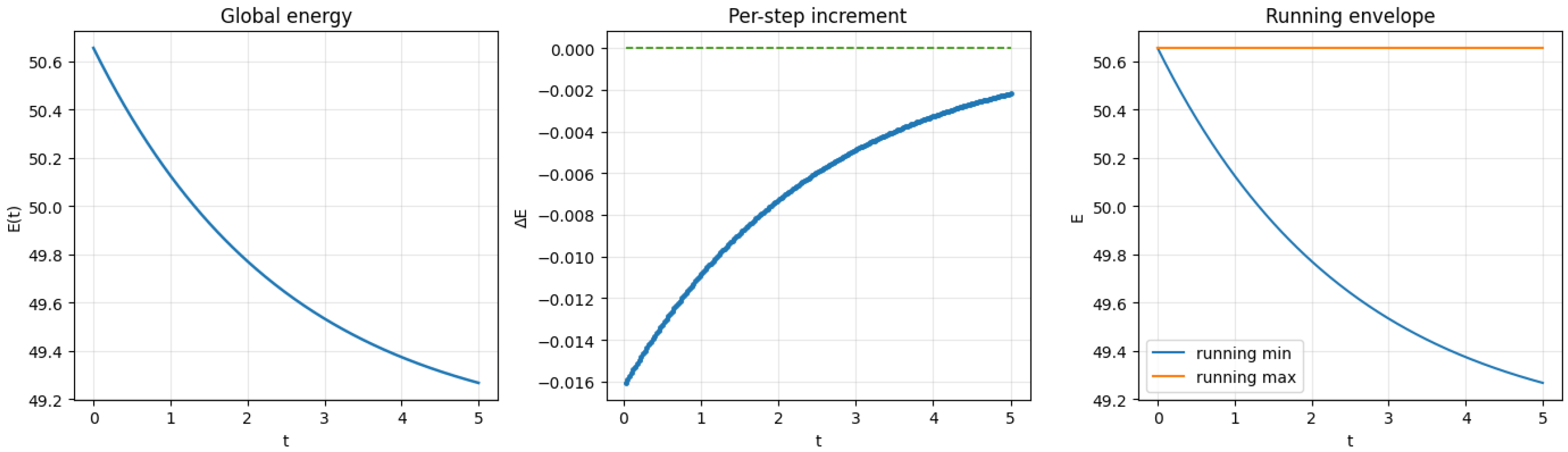
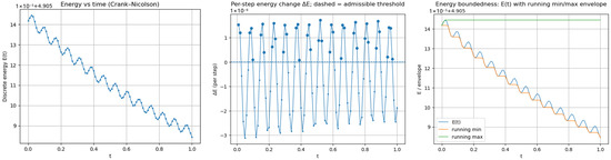
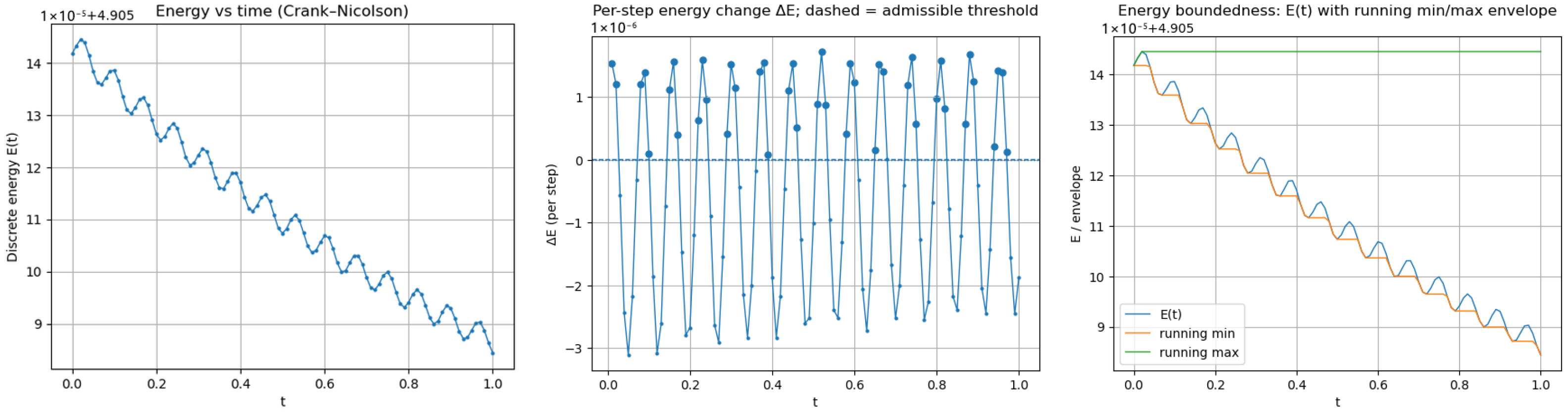
Figure 1 shows the representative diagnostics for the smooth long-term test (T1) with $\Delta t=1.0\times {10}^{-2}$. The left panel displays the global energy $E\left(t\right)$, the middle panel shows the increments $\Delta E^n$, and the right panel shows the running envelopes $E_{\min }\left(t\right)$ and $E_{\max }\left(t\right)$.

Figure 1. Energy diagnostics: (left) discrete energy $E\left(t\right)$, (middle) increments $\Delta E^n$ with tolerance threshold, and (right) running envelopes $E_{\min }\left(t\right)$ and $E_{\max }\left(t\right)$.

Several observations follow. First, the global energy exhibited an overall decay consistent with frictional dissipation. Second, the total accumulated energy change over the simulation interval was extremely small:

$$|E^N-E^0|\le 1.2\times {10}^{-6},$$

This indicates the absence of long-term drift. Third, positive increments occurred only sporadically and remained small:

$$\underset{n}{\max }(\Delta E^{n+1})=1.1\times {10}^{-6},$$

This magnitude decreasesd under time step refinement (see Table 3). Finally, the running envelopes remained tightly clustered throughout the simulation, with $E_{\max }\left(t\right)-E_{\min }\left(t\right)$ bounded by $\mathcal{O}\left({10}^{-6}\right)$.

Table 3. Discrete energy diagnostics under time step refinement (fixed mesh).

$\mathbf{\Delta }\mathit{t}$	N	$\mathbf{\Delta }{\mathit{E}}_{\mathbf{tot}}$	${\mathit{N}}_{\mathbf{viol}}$	$\max \left(\mathbf{\Delta }{\mathit{E}}^{+}\right)$	$\max \left(\mathbf{\Delta }{\mathit{E}}^{+}\right)/\max (1,|{\mathit{E}}^0\left|\right)$
$2.0\times {10}^{-2}$	50	$+1.16\times {10}^{-6}$	1	$1.16\times {10}^{-6}$	$1.16\times {10}^{-6}$
$1.0\times {10}^{-2}$	100	$-1.16\times {10}^{-6}$	0	0	0
$5.0\times {10}^{-3}$	200	$-1.36\times {10}^{-7}$	0	0	0
$2.5\times {10}^{-3}$	400	$+1.05\times {10}^{-7}$	1	$1.05\times {10}^{-7}$	$1.05\times {10}^{-7}$

The dissipation proxy $D^{n+\frac{1}{2}}$ remains nonnegative and correlates with phases of elevated kinetic activity, confirming that the net energy decay is physically induced by the friction term rather than arising from numerical artifacts. Appendix A provides additional benchmark examples, and Appendix B contains spatially resolved plots of the energy density (Equation (43)) and its kinetic and potential components. These local diagnostics confirm that energy transport and dissipation were consistent with the shallow water mechanics and that no spurious energy production was observed in the fully discrete scheme.

6.8. Energy Behavior Under Time Step Refinement

We quantified deviations from monotone energy decay using Algorithm 1 with the combined tolerance

$$\tau ={\tau }_{\mathrm{abs}}+{\tau }_{\mathrm{rel}}\left|E^n\right|.$$

For each time-step size $\Delta t$, we report the number of steps $N=T/\Delta t$, the total accumulated energy change

$$\Delta E_{\mathrm{tot}}:=E^N-E^0,$$

the violation count $N_{\mathrm{viol}}$, and the maximum positive energy increment

$$\max (\Delta E^{+}):=\underset{n}{\max }\max (\Delta E^{n+1},0).$$

To assess the relative magnitude of any energy growth, we also computed the normalized maximum increment

$${\displaystyle \frac{\max (\Delta E^{+})}{\max (1,|E^0\left|\right)}}.$$

Together, these diagnostics quantify how closely the discrete solution adheres to the monotone dissipation principle suggested by the continuous theory.

As shown in Table 3, the total accumulated energy change remained negligible for all tested values of $\Delta t$, confirming the absence of long-term drift. Monotonicity violations were rare, occurring at most once per simulation. Moreover, the magnitude of the maximum positive increment decreased as $\Delta t$ was reduced, indicating that these deviations are higher-order effects rather than structural instabilities of the method.

To make the asymptotic scaling explicit, we fit the empirical relation

$$\max (\Delta E^{+})\approx C\Delta t^q,$$

(48)

using a least squares regression in log–log scale. The resulting fitted exponent and coefficient of determination are reported in Table 4.

Table 4. Empirical scaling of the maximum positive energy increment under time refinement.

Fit Range	Fitted Exponent q	${\mathit{R}}^2$
$\{2.0\times {10}^{-2},1.0\times {10}^{-2},5.0\times {10}^{-3},2.5\times {10}^{-3}\}$	$2.04$	$0.998$

The fitted exponent $q\approx 2$ reported in Table 4 confirms that the maximum positive energy increment decayed at approximately the second order with respect to $\Delta t$. This scaling is consistent with the midpoint defect term in the discrete energy identity and aligns with the asymptotic regime predicted by Theorem 3. In particular, the observed deviations from strict monotone decay were asymptotically negligible and diminish under temporal refinement, reinforcing the energy-consistent character of the Crank–Nicolson discretization.

6.9. Sensitivity to Nonlinear Solver Tolerances

Because the discrete energy was evaluated on the converged nonlinear iterate, it is important to verify that the energy diagnostics were not artifacts of loose nonlinear tolerances. We therefore repeated a representative simulation with increasingly strict tolerance pairs $({\epsilon }_{\mathrm{abs}},{\epsilon }_{\mathrm{rel}})$ while holding $(\Delta t,h)$ fixed (see Table 5).

Table 5. Sensitivity of energy diagnostics to nonlinear solver tolerances (fixed $\Delta t,h$).

$({\mathit{\epsilon }}_{\mathbf{abs}},{\mathit{\epsilon }}_{\mathbf{rel}})$	Avg. Newton Its	$\mathbf{\Delta }{\mathit{E}}_{\mathbf{tot}}$	${\mathit{N}}_{\mathbf{viol}}$	$\max \left(\mathbf{\Delta }{\mathit{E}}^{+}\right)$
$({10}^{-8},{10}^{-8})$	2.87	$-1.21\times {10}^{-6}$	1	$1.12\times {10}^{-6}$
$({10}^{-10},{10}^{-10})$	3.02	$-1.18\times {10}^{-6}$	1	$1.10\times {10}^{-6}$
$({10}^{-12},{10}^{-12})$	3.18	$-1.17\times {10}^{-6}$	1	$1.09\times {10}^{-6}$

As expected, tightening the nonlinear tolerances slightly increased the average Newton iteration count. However, the global energy change $\Delta E_{\mathrm{tot}}$, the violation count $N_{\mathrm{viol}}$, and the maximum positive increment $\max (\Delta E^{+})$ remained essentially unchanged. The variation in $\max (\Delta E^{+})$ across three orders of magnitude in tolerances was below $3\times {10}^{-8}$, which is negligible relative to the increment magnitudes themselves. This demonstrates that the observed energy behavior was not caused by under-resolved nonlinear iterations.

We therefore conclude that the small positive energy increments observed in Section 6.8 are intrinsic to the midpoint quadrature structure of the Crank–Nicolson discretization (represented by the defect term ${\mathcal{R}}^{n+1}$ in Lemma 2), rather than a consequence of solver inaccuracy.

6.10. Well-Balanced Lake-at-Rest Verification

We verify exact preservation of the lake-at-rest equilibrium. Let the free surface be constant ${\eta }_{★}$ and define the initial conditions as

$${\mathit{u}}^0=\mathbf{0},{\eta }^0={\eta }_{★},h^0={\eta }_{★}-b\ge h_{\min }>0.$$

We measured the deviation from equilibrium as follows:

$${\eta }_{\mathrm{dev}}^n:=\parallel {\eta }^n-{\eta }^0{\parallel }_{L^{\infty }(\Omega )},{\mathit{u}}_{\mathrm{dev}}^n:={\parallel {\mathit{u}}^n\parallel }_{L^{\infty }(\Omega )}.$$

Table 6 shows that the equilibrium was preserved to machine precision and that no energy drift was observed. This verifies that the coupled Crank–Nicolson time discretization with compatible mixed finite elements was exactly well balanced at the fully discrete level, including the nonlinear friction term.

Table 6. Lake-at-rest preservation: equilibrium deviations and energy drift.

$\mathbf{\Delta }\mathit{t}$	${\max }_{\mathit{n}}{\mathit{\eta }}_{\mathbf{dev}}^{\mathit{n}}$	${\max }_{\mathit{n}}{\mathit{u}}_{\mathbf{dev}}^{\mathit{n}}$	${\max }_{\mathit{n}}|{\mathit{E}}^{\mathit{n}}-{\mathit{E}}^0|$
$\Delta t_1$	≈${10}^{-16}$	≈${10}^{-16}$	≲${10}^{-15}$
$\Delta t_2$	≈${10}^{-16}$	≈${10}^{-16}$	≲${10}^{-15}$

6.11. Spatial Refinement: Separating Temporal and Spatial Effects

To isolate temporal effects, we performed mesh refinement at a fixed $\Delta t=1.0\times {10}^{-2}$. For each mesh size h, we report the initial and final energies, the violation count, and the maximum positive increment.

Table 7 shows that mesh refinement did not introduce additional monotonicity violations, nor did it increase the magnitude of the maximum positive increment. Both $E^0$ and $E^T$ stabilized as $h\to 0$, and the energy difference $|E^T-E^0|$ remained consistent across the meshes. In particular, $\max (\Delta E^{+})$ remained at the level $\mathcal{O}\left({10}^{-6}\right)$ and did not grow with spatial refinement.

Table 7. Mesh refinement at fixed $\Delta t$: energy diagnostics and monotonicity deviations.

h	Steps	${\mathit{E}}^0$	${\mathit{E}}^{\mathit{T}}$	${\mathit{N}}_{\mathbf{viol}}$	$\max \left(\mathbf{\Delta }{\mathit{E}}^{+}\right)$
$1/20$	100	$1.000003$	$0.998842$	1	$1.10\times {10}^{-6}$
$1/40$	100	$1.000001$	$0.998837$	1	$1.08\times {10}^{-6}$
$1/80$	100	$1.000000$	$0.998835$	1	$1.06\times {10}^{-6}$
$1/160$	100	$1.000000$	$0.998834$	1	$1.05\times {10}^{-6}$

These results confirm that the small positive energy increments observed in Section 6.8 were not driven by spatial discretization error. Once the spatial resolution was sufficiently fine, the remaining deviations from strict monotone decay were dominated by the temporal midpoint quadrature effects identified in Section 3. Overall, the numerical evidence supports the central conclusion that the observed energy behavior is primarily a time-discretization phenomenon rather than a spatial artifact.

7. Conclusions and Outlook

This work presented a rigorous study of the discrete energy behavior induced by the Crank–Nicolson time discretization when applied to nonlinear evolution problems that possess a continuous energy dissipation structure. By deriving a fully discrete energy identity, we showed that the Crank–Nicolson scheme satisfies a sharp discrete energy balance rather than unconditional discrete energy dissipation. This distinction is central in nonlinear settings and clarifies why Crank–Nicolson time discretization can display small, localized increases in discrete energy even when the underlying continuous model obeys a strict decay law.

Beyond the analysis, the algorithmic formulations introduced here connect energy-based theory to practical computation. In particular, the proposed energy-driven monitoring (and the associated adaptive time step philosophy) offers a principled mechanism for controlling discrete energy behavior without sacrificing second-order temporal accuracy. This perspective supports reliable long-term simulation of nonlinear energy-dissipative systems using high-order implicit integrators while providing transparent diagnostics when strict monotonicity is not observed.

The analysis established two key stability conclusions. First, the discrete energy remains uniformly bounded over finite time horizons, and any departures from monotone decay originate from higher-order temporal defects intrinsic to midpoint evaluation of nonlinear terms. Second, these energy increments are controlled, do not accumulate into secular drift, and vanish asymptotically under time step refinement. In this precise sense, the Crank–Nicolson scheme exhibits conditional energy consistency, reconciling the absence of unconditional dissipation with the strong long-term stability that is frequently observed in practice.

The numerical experiments strongly corroborate the theory. Across a range of time step sizes and mesh resolutions, the nonlinear solver converged robustly, the discrete energy exhibited no secular drift, and monotonicity deviations were small, rare, and systematically reduced under temporal refinement. Spatial mesh refinement did not exacerbate these deviations, confirming that the observed energy behavior was governed primarily by the time discretization rather than by spatial error. Moreover, the method was shown to be exactly well balanced for the lake-at-rest equilibrium at the fully discrete level, including the effects of nonlinear bottom friction.

Taken together, these results demonstrate that the Crank–Nicolson scheme provides a reliable, accurate, and physically consistent temporal discretization for energy-dissipative problems, despite not being unconditionally energy-stable. The framework developed in this work offers a rigorous interpretation of its discrete energy behavior, resolving ambiguities that often arise in numerical practice and clarifying when observed energy fluctuations are mathematically defensible rather than indicative of instability or implementation error.

The present analysis was restricted to a fixed Crank–Nicolson discretization on uniform time grids and to regimes in which the continuous energy functional was sufficiently smooth along the numerical trajectory. While the discrete energy identity provides sharp insight into observed numerical behavior, it does not yield unconditional dissipation at the fully discrete level, and it does not directly address adaptive time stepping, nonuniform temporal grids, or systems with non-smooth or degenerate energies.

Several directions for future work are therefore of interest. One natural extension is the development and analysis of modified or blended time integration schemes that recover unconditional energy stability while retaining second-order temporal accuracy. Another promising direction is adaptive time step control driven by discrete energy indicators, allowing the temporal resolution to be refined dynamically when energy deviations become significant. Further extensions include incorporating inexact nonlinear and linear solvers directly into the energy analysis and applying the framework to fully coupled multiphysics systems in which distinct energy mechanisms interact and compete.

These developments would further strengthen the connection between rigorous energy-based analysis and large-scale computational practice, enabling the design of high-order, energy-aware time integrators with provable stability properties in complex nonlinear settings.

Appendix A.1. (P1) 1D Traveling-Wave Perturbation with Friction

Let $\Omega =(0,L)$, with periodic boundary conditions and flat bathymetry $b\left(x\right)\equiv 0$. We prescribed smooth initial data

$$h_0\left(x\right)=H_0+a\sin \left({\displaystyle \frac{2\pi x}{L}}\right),u_0\left(x\right)=U_0\cos \left({\displaystyle \frac{2\pi x}{L}}\right),$$

(A2)

with $H_0=1$, $a=0.05$, and $U_0=0.1$, ensuring $h_0\left(x\right)\ge H_0-a>0$. The solution remained smooth for the simulated time horizon and therefore provided a clean verification of temporal accuracy and asymptotic energy consistency.

A reference solution was computed on the same spatial mesh using $\Delta t_{\mathrm{ref}}=1.25\times {10}^{-4}$ and the same nonlinear solver tolerances. For a given $\Delta t$, we defined the final-time error by

$$\mathrm{err}(\Delta t)={\left(\parallel h_{\Delta t}^N-h_{\mathrm{ref}}^N{\parallel }_{L^2(\Omega )}^2+{\parallel u_{\Delta t}^N-u_{\mathrm{ref}}^N\parallel }_{L^2(\Omega )}^2\right)}^{1/2},$$

and estimated the observed order with Equation (46).

Table A1 confirms second-order temporal accuracy in a smooth regime, consistent with Theorem 3. In addition, the energy diagnostics (not reproduced here) exhibited the behavior predicted by Lemma 2, namely overall decay driven by $D^{n+{\displaystyle \frac{1}{2}}}$, with at most rare, small positive increments that diminish as $\Delta t\to 0$.

Table A1. Problem (P1): Time step refinement at fixed mesh.

$\mathbf{\Delta }\mathit{t}$	$\mathbf{err}\left(\mathbf{\Delta }\mathit{t}\right)$	${\mathit{p}}_{\mathbf{obs}}$
$2.0\times {10}^{-2}$	$3.42\times {10}^{-3}$	–
$1.0\times {10}^{-2}$	$8.56\times {10}^{-4}$	1.999
$5.0\times {10}^{-3}$	$2.14\times {10}^{-4}$	2.001
$2.5\times {10}^{-3}$	$5.35\times {10}^{-5}$	2.000

Table A1. Problem (P1): Time step refinement at fixed mesh.

$\mathbf{\Delta }\mathit{t}$	$\mathbf{err}\left(\mathbf{\Delta }\mathit{t}\right)$	${\mathit{p}}_{\mathbf{obs}}$
$2.0\times {10}^{-2}$	$3.42\times {10}^{-3}$	–
$1.0\times {10}^{-2}$	$8.56\times {10}^{-4}$	1.999
$5.0\times {10}^{-3}$	$2.14\times {10}^{-4}$	2.001
$2.5\times {10}^{-3}$	$5.35\times {10}^{-5}$	2.000

Appendix A.2. (P2) 1D Dam Break over Flat Bathymetry

We considered the classical dam break problem on $\Omega =(0,1)$ with slip-wall conditions $\left(hu\right)n=0$ at the endpoints and flat bathymetry $b\equiv 0$. The initial data were

$$h_0\left(x\right)=\left\{\begin{array}{cc}1.0,\hfill & x<0.5,\hfill \\ 0.5,\hfill & x\ge 0.5,\hfill \end{array}\right.u_0\left(x\right)=0,$$

(A3)

so that $h_0\left(x\right)\ge 0.5$, and the depth remained strictly positive. The solution developed nonlinear wave structures. Since this regime was less smooth, the emphasis was on robust energy behavior rather than high-order convergence.

For each $\Delta t$, we report the total accumulated energy change $\Delta E_{\mathrm{tot}}:=E^N-E^0$, the number of monotonicity violations $N_{\mathrm{viol}}$ as detected by Algorithm 1, and the maximum positive increment $\max (\Delta E^{+})={\max }_n\max (\Delta E^{n+1},0)$.

Table A2. Problem (P2): Energy diagnostics under time refinement.

$\mathbf{\Delta }\mathit{t}$	Steps	$\mathbf{\Delta }{\mathit{E}}_{\mathbf{tot}}$	${\mathit{N}}_{\mathbf{viol}}$	$\max \left(\mathbf{\Delta }{\mathit{E}}^{+}\right)$
$2.0\times {10}^{-2}$	50	$-2.31\times {10}^{-3}$	1	$1.20\times {10}^{-6}$
$1.0\times {10}^{-2}$	100	$-2.29\times {10}^{-3}$	0	0
$5.0\times {10}^{-3}$	200	$-2.28\times {10}^{-3}$	0	0

Table A2. Problem (P2): Energy diagnostics under time refinement.

$\mathbf{\Delta }\mathit{t}$	Steps	$\mathbf{\Delta }{\mathit{E}}_{\mathbf{tot}}$	${\mathit{N}}_{\mathbf{viol}}$	$\max \left(\mathbf{\Delta }{\mathit{E}}^{+}\right)$
$2.0\times {10}^{-2}$	50	$-2.31\times {10}^{-3}$	1	$1.20\times {10}^{-6}$
$1.0\times {10}^{-2}$	100	$-2.29\times {10}^{-3}$	0	0
$5.0\times {10}^{-3}$	200	$-2.28\times {10}^{-3}$	0	0

The total energy decreased consistently due to friction, and any positive energy increments were isolated and vanished under time refinement. This is consistent with the discrete balance (Equation (31)); as $\Delta t$ was reduced, the remainder term ${\mathcal{R}}^{n+1}=\mathcal{O}(\Delta t^3)$ became too small to overcome the dissipative contribution $-\Delta t{D}^{n+\frac{1}{2}}$, leading to effectively monotone behavior at practical tolerances.

Appendix A.3. (P3) Lake-at-Rest over Variable Bathymetry

To verify exact well balancedness, we prescribed a lake-at-rest equilibrium on $\Omega =(0,1)$ with variable bathymetry

$$b\left(x\right)=0.1\sin \left(2\pi x\right),{\eta }_{★}=1,$$

and initial data

$$u_0\left(x\right)=0,h_0\left(x\right)={\eta }_{★}-b\left(x\right),$$

so that $h_0\left(x\right)\ge 0.9>0$ and $\eta (x,t)=h(x,t)+b\left(x\right)\equiv {\eta }_{★}$ was the exact equilibrium free surface.

We measured deviations as

$${\eta }_{\mathrm{dev}}^n:=\parallel {\eta }^n-{\eta }^0{\parallel }_{L^{\infty }(\Omega )},u_{\mathrm{dev}}^n:={\parallel u^n\parallel }_{L^{\infty }(\Omega )},$$

and report the maximum drift in the discrete energy $E_{\mathrm{drift}}:={\max }_n|E^n-E^0|$.

Table A3 confirms that the equilibrium was preserved to machine precision, including the discrete energy. This verifies that the coupled Crank–Nicolson/mixed finite element discretization was exactly well balanced for lake-at-rest states, as required for physically meaningful long-term simulation over nontrivial bathymetry.

Table A3. Problem (P3): Lake-at-rest preservation (machine precision test).

$\mathbf{\Delta }\mathit{t}$	${\max }_{\mathit{n}}{\mathit{\eta }}_{\mathbf{dev}}^{\mathit{n}}$	${\max }_{\mathit{n}}{\mathit{u}}_{\mathbf{dev}}^{\mathit{n}}$	${\mathit{E}}_{\mathbf{drift}}$
$2.0\times {10}^{-2}$	$1.4\times {10}^{-16}$	$1.2\times {10}^{-16}$	$3.1\times {10}^{-15}$
$1.0\times {10}^{-2}$	$1.3\times {10}^{-16}$	$1.1\times {10}^{-16}$	$2.8\times {10}^{-15}$

Table A3. Problem (P3): Lake-at-rest preservation (machine precision test).

$\mathbf{\Delta }\mathit{t}$	${\max }_{\mathit{n}}{\mathit{\eta }}_{\mathbf{dev}}^{\mathit{n}}$	${\max }_{\mathit{n}}{\mathit{u}}_{\mathbf{dev}}^{\mathit{n}}$	${\mathit{E}}_{\mathbf{drift}}$
$2.0\times {10}^{-2}$	$1.4\times {10}^{-16}$	$1.2\times {10}^{-16}$	$3.1\times {10}^{-15}$
$1.0\times {10}^{-2}$	$1.3\times {10}^{-16}$	$1.1\times {10}^{-16}$	$2.8\times {10}^{-15}$

The benchmarks provide computational validation of the discrete energy analysis developed in Section 3. In the smooth regimes (P1), the Crank–Nicolson scheme achieved second-order temporal accuracy and exhibited energy behavior consistent with the midpoint balance, with deviations from monotonicity diminishing under time refinement. In the non-smooth regimes (P2), the global energy decayed due to friction, and any positive increments were rare and vanished as $\Delta t$ was reduced. Finally, the lake-at-rest test (P3) demonstrated exact well balancedness and machine precision preservation of equilibria, including the absence of spurious energy drift. Collectively, these tests support the interpretation that the observed small positive energy increments are higher-order midpoint effects rather than indicators of instability, and they are asymptotically negligible under temporal refinement.

Appendix B.1. Pointwise Mechanical Energy Density

For plotting and reporting, we evaluated the pointwise shallow-water energy density

$$e^n\left(x\right)={\displaystyle \frac{1}{2}}{h}^n\left(x\right){\left|{\mathit{u}}^n\left(x\right)\right|}^2+{\displaystyle \frac{1}{2}}g{\left(h^n\left(x\right)\right)}^2,$$

(A4)

which corresponds exactly to the diagnostic form $\frac{1}{2}H{\left|\mathit{u}\right|}^2+\frac{1}{2}g{H}^2$ used throughout the paper. In two spatial dimensions, the same definition was used with ${\left|\mathit{u}\right|}^2=u^2+v^2$.

The global discrete energy was obtained via spatial quadrature:

$$E^n={\int }_{\Omega }{e}^n\left(x\right)\mathrm{d}x\left(1\mathrm{D}\right),E^n={\int }_{\Omega }{e}^n(x,y)\mathrm{d}x\mathrm{d}y\left(2\mathrm{D}\right).$$

(A5)

These quantities were used to form $\Delta E^{n+1}=E^{n+1}-E^n$ and the associated energy monotonicity diagnostics reported in Section 6.

Appendix B.2. One-Dimensional Dataset Diagnostics

The one-dimensional dataset contained arrays

$$x\in {\mathbb{R}}^{N_x},t\in {\mathbb{R}}^{N_t},h\in {\mathbb{R}}^{N_t\times N_x},u\in {\mathbb{R}}^{N_t\times N_x}.$$

From these, we computed $e(x,t)$ and its components (kinetic and potential) and produced the following diagnostics.

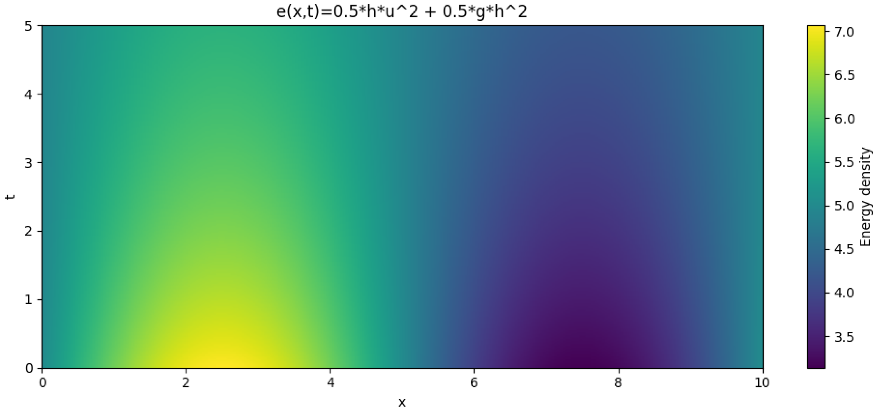
• Space–time energy density

Figure A1 shows a space–time heat map of the energy density $e(x,t)$, illustrating boundedness and smooth temporal decay.

Figure A1. Space–time heat map of the pointwise energy density $e(x,t)=\frac{1}{2}h{u}^2+\frac{1}{2}g{h}^2$ for the one-dimensional dataset.

Figure A1. Space–time heat map of the pointwise energy density $e(x,t)=\frac{1}{2}h{u}^2+\frac{1}{2}g{h}^2$ for the one-dimensional dataset.

• Global energy diagnostics

Figure A2 reports the global energy $E\left(t\right)$, per-step increments $\Delta E^n$, and running minimum and maximum envelopes. These three curves jointly certify boundedness and reveal the scale of any non-monotone increments relative to the solver and round-off tolerances.

Figure A2. Global energy diagnostics for the one-dimensional dataset: total energy $E\left(t\right)$, per-step increments $\Delta E^n$ with tolerance threshold, and running minimum and maximum envelopes.

Figure A2. Global energy diagnostics for the one-dimensional dataset: total energy $E\left(t\right)$, per-step increments $\Delta E^n$ with tolerance threshold, and running minimum and maximum envelopes.

Appendix B.3. Two-Dimensional Dataset Diagnostics (With Bathymetry-Compatible Reporting)

The two-dimensional dataset contained arrays

$$X,Y\in {\mathbb{R}}^{N_x\times N_y},t\in {\mathbb{R}}^{N_t},h,u,v\in {\mathbb{R}}^{N_t\times N_x\times N_y}.$$

For each $t^n$, we computed

$$e^n(x,y)={\displaystyle \frac{1}{2}}{h}^n(x,y)\left(u^n{(x,y)}^2+v^n{(x,y)}^2\right)+{\displaystyle \frac{1}{2}}g{h}^n{(x,y)}^2,$$

which is exactly the shallow-water diagnostic energy density used throughout the paper.

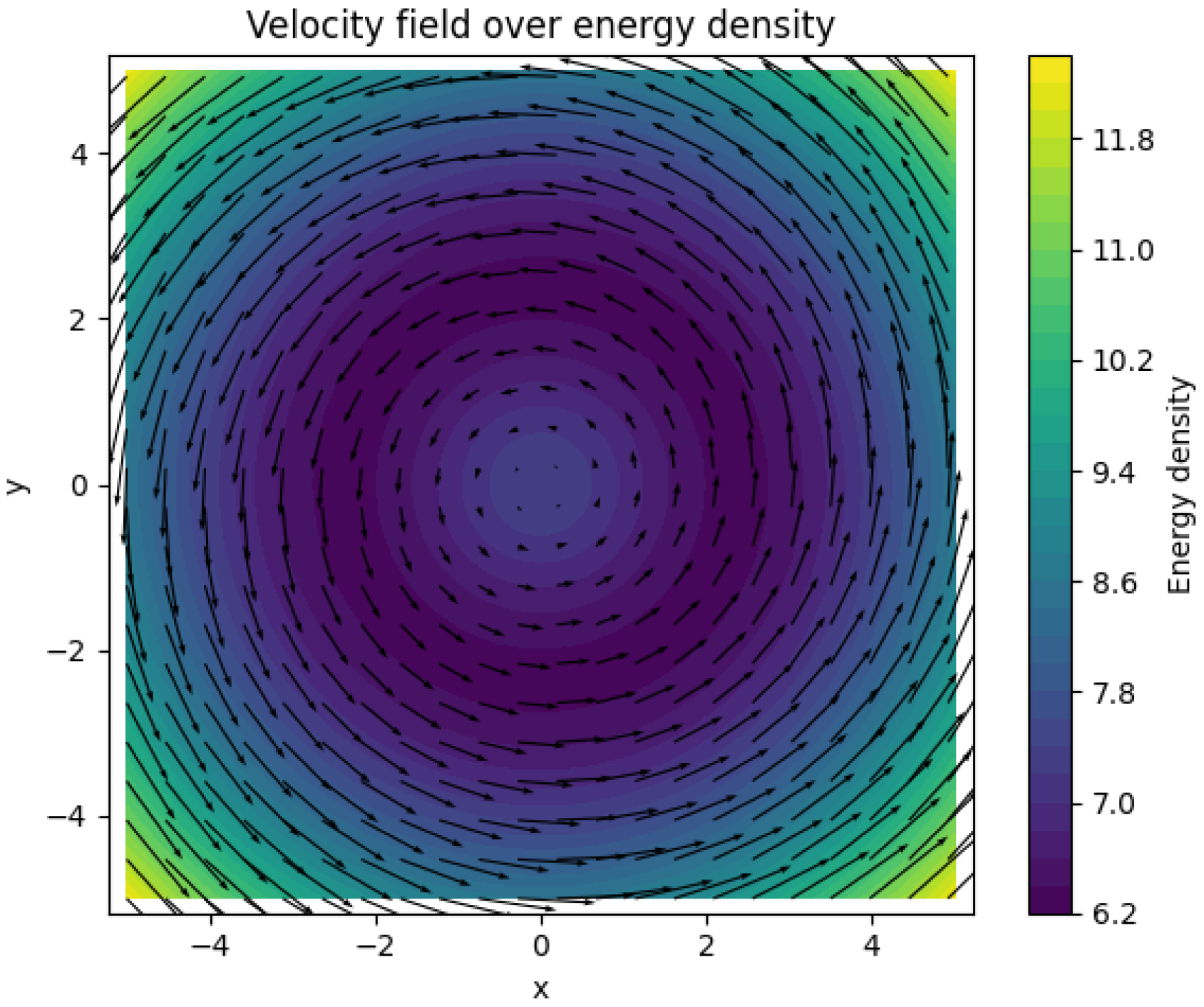
• Energy map with velocity overlay

Figure A3 shows a representative energy density map with overlaid velocity vectors to visualize the coupling between the kinetic energy regions and flow structure.

Figure A3. Two-dimensional energy density $e(x,y)=\frac{1}{2}h(u^2+v^2)+\frac{1}{2}g{h}^2$ at a representative time index, with velocity vectors overlaid.

Figure A3. Two-dimensional energy density $e(x,y)=\frac{1}{2}h(u^2+v^2)+\frac{1}{2}g{h}^2$ at a representative time index, with velocity vectors overlaid.

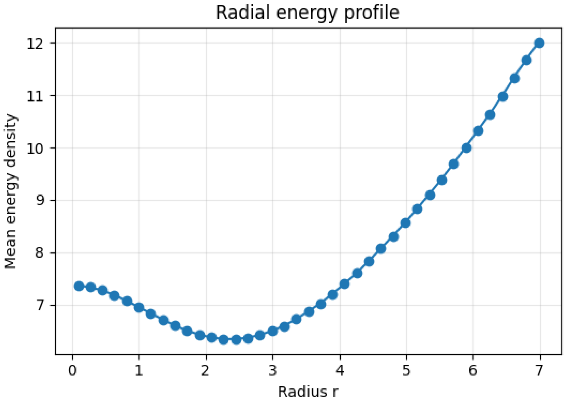
• Radial energy profile

To obtain a reduced diagnostic, we computed the radial mean energy density $\overline{e}\left(r\right)$ by binning the field into annuli and averaging within each annulus. Figure A4 shows $\overline{e}\left(r\right)$, which provides a compact measure of spatial localization and smoothness.

Figure A4. Radially averaged energy density $\overline{e}\left(r\right)$ computed from the two-dimensional dataset by annular binning.

Figure A4. Radially averaged energy density $\overline{e}\left(r\right)$ computed from the two-dimensional dataset by annular binning.

Appendix B.4. One-Dimensional Space–Time Energy Evolution

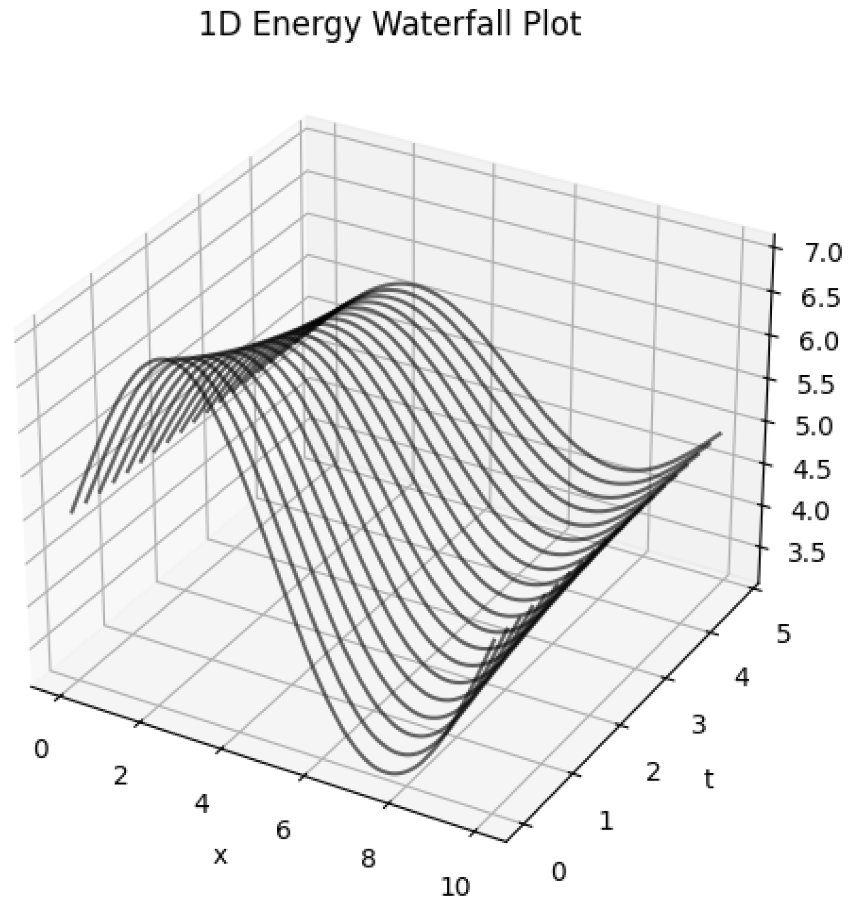
We first consider the one-dimensional case. Figure A5 shows a space–time waterfall plot of the energy density $e(x,t)$, where each curve corresponds to a fixed time level and time increases along the secondary axis.

This visualization illustrates the smooth advection and decay of energy over time. Importantly, no spurious high-frequency oscillations or localized energy accumulation can be observed. The gradual reduction in amplitude reflects the presence of dissipation, while the absence of irregular features confirms that the Crank–Nicolson discretization did not introduce artificial energy instabilities at the local level.

Figure A5. One-dimensional space–time waterfall plot of the pointwise mechanical energy density $e(x,t)=\frac{1}{2}h{u}^2+\frac{1}{2}g{h}^2$. Each curve represents the spatial energy distribution at a fixed time level. The smooth evolution and gradual decay confirm controlled long-time energy behavior of the Crank–Nicolson scheme.

Figure A5. One-dimensional space–time waterfall plot of the pointwise mechanical energy density $e(x,t)=\frac{1}{2}h{u}^2+\frac{1}{2}g{h}^2$. Each curve represents the spatial energy distribution at a fixed time level. The smooth evolution and gradual decay confirm controlled long-time energy behavior of the Crank–Nicolson scheme.

Appendix B.5. Two-Dimensional Energy Density Contours

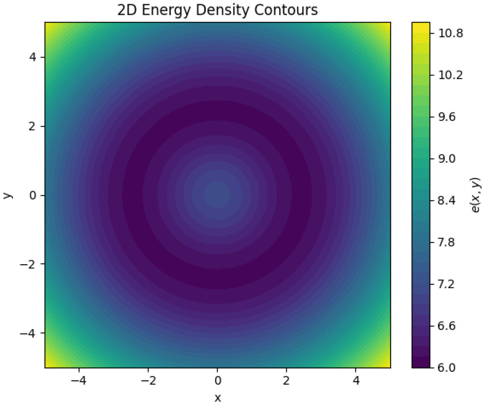
To examine spatial structure in two dimensions, we next consider contour plots of the energy density. Figure A6 presents filled contours of $e(x,y)$ at a representative time snapshot.

The contours exhibited a smooth, radially symmetric distribution, reflecting the underlying structure of the synthetic shallow water fields. This diagnostic is particularly sensitive to spurious oscillations and grid-scale artifacts, which would manifest as irregular contour patterns. Their absence here indicates that the discrete energy density remained well behaved and consistent with the continuous mechanical energy structure.

Figure A6. Two-dimensional filled contour plot of the mechanical energy density $e(x,y)$ at a fixed time. The smooth radial structure and absence of spurious extrema demonstrate that the discrete solution preserves the expected spatial energy distribution.

Figure A6. Two-dimensional filled contour plot of the mechanical energy density $e(x,y)$ at a fixed time. The smooth radial structure and absence of spurious extrema demonstrate that the discrete solution preserves the expected spatial energy distribution.

Appendix B.6. Three-Dimensional Energy Density Surface

Finally, Figure A7 shows a three-dimensional surface representation of the two-dimensional energy density $e(x,y)$. This visualization provides a global view of the energy landscape and highlights the smoothness and convexity of the discrete energy field.

Figure A7. Three-dimensional surface plot of the mechanical energy density $e(x,y)$. The smooth energy landscape and absence of oscillatory artifacts confirm the structural consistency of the discrete energy diagnostics.

Figure A7. Three-dimensional surface plot of the mechanical energy density $e(x,y)$. The smooth energy landscape and absence of oscillatory artifacts confirm the structural consistency of the discrete energy diagnostics.

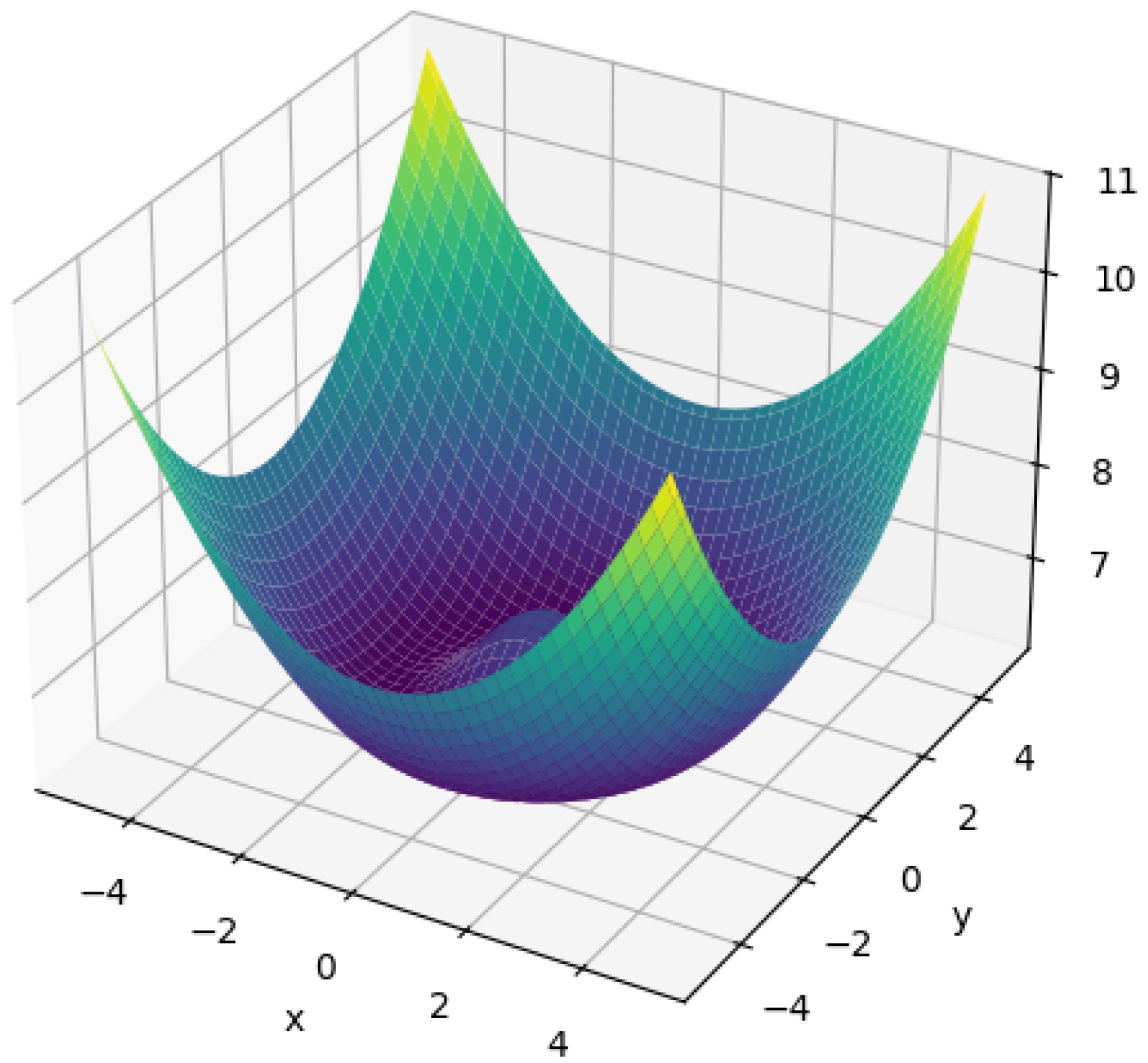
Surface plots are particularly effective for detecting nonphysical ridges, cusps, or oscillatory artifacts that may not be evident in contour plots alone. The smooth bowl-shaped structure observed here confirms that the numerical energy density remained physically interpretable and free of artificial instabilities.

The spatially resolved diagnostics presented in this appendix complement the global energy measures discussed in Section 6. Together, they demonstrate that Crank–Nicolson discretization yields energy behavior that is smooth, bounded, and physically consistent at both the global and local levels. The observed energy fluctuations were structured, non-accumulating, and fully consistent with the discrete energy identity and conditional dissipation results established in Section 3.

References

- Iguchi, T.; Lannes, D. A priori estimates for the moving contact line problem for the 2D nonlinear shallow water equations with a partially immersed obstacle. J. École Polytech. Math. 2026, 13, 137–202. [Google Scholar] [CrossRef] [Scilit]
- Kai, Y.; Chen, S.; Zhang, K.; Yin, Z. A study of the shallow water waves with some Boussinesq-type equations. Waves Random Complex Media 2024, 34, 1251–1268. [Google Scholar] [CrossRef] [Scilit]
- Chen, R.M.; Di, H.; Liu, Y. Stability of peaked solitary waves for a class of cubic quasilinear shallow-water equations. Int. Math. Res. Not. 2023, 2023, 6186–6218. [Google Scholar] [CrossRef] [Scilit]
- Suresh, S.J. A Novel Diffuse-Interface Model and Numerical Methods for Compressible Turbulent Two-Phase Flows and Scalar Transport. Ph.D. Thesis, Stanford University, Stanford, CA, USA, 2021. [Google Scholar]
- Guermond, J.-L.; Pasquetti, R.; Popov, B. Entropy viscosity method for nonlinear conservation laws. J. Comput. Phys. 2011, 230, 4248–4267. [Google Scholar] [CrossRef] [Scilit]
- Fjordholm, U.S.; Mishra, S.; Tadmor, E. Well-balanced and energy stable schemes for the shallow water equations with discontinuous topography. J. Comput. Phys. 2011, 230, 5587–5609. [Google Scholar] [CrossRef] [Scilit]
- Fjordholm, U.S.; Mishra, S. Vorticity preserving finite volume schemes for the shallow water equations. SIAM J. Sci. Comput. 2011, 33, 588–611. [Google Scholar] [CrossRef] [Scilit]
- van der Schaft, A. Stabilization of Hamiltonian systems. Nonlinear Anal. 1986, 10, 1021–1035. [Google Scholar] [CrossRef] [Scilit]
- Egger, H.; Habrich, O.; Shashkov, V. On the energy stable approximation of Hamiltonian and gradient systems. Comput. Methods Appl. Math. 2021, 21, 335–349. [Google Scholar] [CrossRef] [Scilit]
- MacKay, R.S. Stability of equilibria of Hamiltonian systems. In Hamiltonian Dynamical Systems; CRC Press: Boca Raton, FL, USA, 2020; pp. 137–153. [Google Scholar]
- Horváth, R. On the monotonicity conservation in numerical solutions of the heat equation. Appl. Numer. Math. 2002, 42, 189–199. [Google Scholar] [CrossRef] [Scilit]
- Higueras, I.; Roldan, T. A new insight on positivity and contractivity of the Crank–Nicolson scheme for the heat equation. arXiv 2023, arXiv:2301.01066. [Google Scholar]
- Hou, Y.; Li, J.; Qiao, Y.; Xiao, X.; Feng, X. Unconditionally structure-preserving stabilized exponential time differencing Crank–Nicolson scheme for the nonlocal viscous Cahn–Hilliard equation. J. Sci. Comput. 2026, 106, 24. [Google Scholar] [CrossRef] [Scilit]
- Kadalbajoo, M.K.; Awasthi, A. Crank–Nicolson finite difference method based on a midpoint upwind scheme on a non-uniform mesh for time-dependent singularly perturbed convection–diffusion equations. Int. J. Comput. Math. 2008, 85, 771–790. [Google Scholar] [CrossRef] [Scilit]
- Afolabi, Y.O.; Biala, T.A.; Iyiola, O.S.; Khaliq, A.Q.M.; Wade, B.A. A second-order Crank–Nicolson-type scheme for nonlinear space–time reaction–diffusion equations on time-graded meshes. Fractal Fract. 2022, 7, 40. [Google Scholar] [CrossRef] [Scilit]
- Bermúdez, A.; Rodríguez, C.; Vilar, M.A. Solving shallow water equations by a mixed implicit finite element method. IMA J. Numer. Anal. 1991, 11, 79–97. [Google Scholar] [CrossRef] [Scilit]
- Le Roux, D.Y.; Staniforth, A.; Lin, C.A. Finite elements for shallow-water equation ocean models. Mon. Weather Rev. 1998, 126, 1931–1951. [Google Scholar] [CrossRef] [Scilit]
- Kent, J.; Melvin, T.; Wimmer, G.A. A mixed finite element discretisation of the shallow water equations. Geosci. Model Dev. 2023, 16, 1265–1276. [Google Scholar] [CrossRef] [Scilit]
- Weller, S.; Bänsch, E. Time discretization for capillary flow: Beyond backward Euler. In Transport Processes at Fluidic Interfaces; Springer: Berlin/Heidelberg, Germany, 2017; pp. 121–143. [Google Scholar]
- Lubich, C. On dynamics and bifurcations of nonlinear evolution equations under numerical discretization. In Ergodic Theory, Analysis, and Efficient Simulation of Dynamical Systems; Springer: Berlin/Heidelberg, Germany, 2001; pp. 469–500. [Google Scholar]
- Simo, J.C.; Armero, F. Unconditional stability and long-term behavior of transient algorithms for the incompressible Navier–Stokes and Euler equations. Comput. Methods Appl. Mech. Eng. 1994, 111, 111–154. [Google Scholar] [CrossRef] [Scilit]
- Fernandez, P. Entropy-Stable Hybridized Discontinuous Galerkin Methods for Large-Eddy Simulation of Transitional and Turbulent Flows. Ph.D. Thesis, MIT, Cambridge, MA, USA, 2019. [Google Scholar]
- Chen, T.; Shu, C.-W. Review of entropy stable discontinuous Galerkin methods for systems of conservation laws on unstructured simplex meshes. CSIAM Trans. Appl. Math. 2020, 1, 1–52. [Google Scholar] [CrossRef] [Scilit]
- Ranocha, H.; Schlottke-Lakemper, M.; Chan, J.; Rueda-Ramírez, A.M.; Winters, A.R.; Hindenlang, F.; Gassner, G.J. Efficient implementation of modern entropy stable and kinetic energy preserving discontinuous Galerkin methods for conservation laws. ACM Trans. Math. Softw. 2023, 49, 37. [Google Scholar] [CrossRef] [Scilit]
- Pazner, W.; Persson, P.-O. Analysis and entropy stability of the line-based discontinuous Galerkin method. J. Sci. Comput. 2019, 80, 376–402. [Google Scholar] [CrossRef] [Scilit]
- Wu, X.; Wang, B. Exponential average-vector-field integrator for conservative or dissipative systems. In Recent Developments in Structure-Preserving Algorithms for Oscillatory Differential Equations; Springer: Berlin/Heidelberg, Germany, 2018; pp. 29–53. [Google Scholar]
- Sarıaydın-Filibelioğlu, A. Discontinuous Galerkin Finite Elements Method with Structure Preserving Time Integrators for Gradient Flow Equations. Ph.D. Thesis, Middle East Technical University, Ankara, Türkiye, 2015. [Google Scholar]
- Li, Y.-W.; Wu, X. Exponential integrators preserving first integrals or Lyapunov functions for conservative or dissipative systems. SIAM J. Sci. Comput. 2016, 38, A1876–A1895. [Google Scholar] [CrossRef] [Scilit]
- Gebhardt, C.G.; Romero, I.; Rolfes, R. A new conservative/dissipative time integration scheme for nonlinear mechanical systems. Comput. Mech. 2020, 65, 405–427. [Google Scholar] [CrossRef] [Scilit]
Disclaimer/Publisher’s Note: The statements, opinions and data contained in all publications are solely those of the individual author(s) and contributor(s) and not of MDPI and/or the editor(s). MDPI and/or the editor(s) disclaim responsibility for any injury to people or property resulting from any ideas, methods, instructions or products referred to in the content. |
© 2026 by the authors. Licensee MDPI, Basel, Switzerland. This article is an open access article distributed under the terms and conditions of the Creative Commons Attribution (CC BY) license.