Article

An Evolutionary Neural-Enhanced Intelligent Controller for Robotic Visual Servoing Under Non-Gaussian Noise

1
School of Electrical and Electronic Engineering, Changchun University of Technology, Changchun 130012, China
2
Zhejiang Petrochemical Co., Ltd., Zhoushan 316000, China
*
Author to whom correspondence should be addressed.
Mathematics 2026, 14(4), 653; https://doi.org/10.3390/math14040653
Submission received: 29 December 2025 / Revised: 1 February 2026 / Accepted: 10 February 2026 / Published: 12 February 2026

Abstract

Accurate state estimation is essential for the performance of uncalibrated visual servoing systems, yet it is frequently undermined by non-Gaussian disturbances—such as impulse noise, motion blur, and occlusions—whose heavy-tailed statistical characteristics are not adequately represented by conventional Gaussian models. To address this issue, this paper presents an evolutionary neural-enhanced intelligent controller designed for robotic visual servoing under such noise conditions. The controller architecture incorporates a hybrid estimation core that integrates α -stable distribution modeling for principled noise characterization with an Interacting Multiple Model Kalman filter (IMM-KF) to address system dynamics and uncertainties. A multi-layer perceptron (MLP), optimized globally via the Stochastic Fractal Search (SFS) algorithm, is embedded to provide adaptive compensation for residual estimation errors. This integration of statistical modeling, adaptive filtering, and evolutionary optimization constitutes a coherent learning-based control framework. Simulations and physical experiments reveal that the proposed method enhances improvements in estimation accuracy and tracking performance relative to conventional approaches. The outcomes indicate that the framework offers a functional solution for vision-based robotic systems operating under realistic conditions where non-Gaussian sensor noise is present.

1. Introduction

The development of intelligent control systems for robotics represents a core pursuit in modern industrial automation, with visual servoing standing as a pivotal technology that enables high-precision positioning and assembly through the integration of computer vision and real-time motion control [1,2,3,4,5]. These systems are foundational in applications ranging from automotive manufacturing to microelectronics and medical devices, where tasks such as micrometer-level engine alignment and delicate component handling demand exceptional accuracy and reliability [6,7,8]. The performance of such a vision-guided system fundamentally depends on accurate state estimation, which directly determines the precision of its closed-loop control [9,10].
However, achieving robust and precise state estimation in real-world industrial settings remains a significant challenge, primarily due to the presence of non-Gaussian disturbances. Measurement corruption from sensor-induced impulse noise, motion blur, and intermittent occlusions introduces errors with heavy-tailed and impulsive statistical characteristics that fundamentally violate the Gaussian noise assumption underlying conventional estimation algorithms, such as the standard Kalman filter [11,12]. This mismatch leads to substantial degradation in the estimation of the image Jacobian matrix, resulting in feature tracking failures, reduced positioning accuracy, and ultimately, a limitation on the system’s operational robustness in demanding environments.

1.1. Related Work

In image-based visual servoing systems, non-Gaussian noise such as pulse noise and exponential noise primarily caused by sensor failures, feature mismatches, and occlusions [13,14] permeates all stages of image acquisition, transmission, and processing. This noise not only reduces the accuracy of feature extraction but also increases feature error bias. More severely, it can distort the image Jacobian matrix, ultimately leading to servoing task failure. To meet stringent system stability requirements, improving control accuracy and robustness against non-Gaussian noise is crucial. Precise estimation of the image Jacobian matrix is the key technology for noise suppression and stability assurance. It is currently achieved through mainstream nonlinear optimization and state estimation methods, which aim to enhance the estimation accuracy and robustness of the matrix (or its pseudoinverse) [15,16,17,18].
Nonlinear optimization methods transform the visual servoing problem into a nonlinear least-squares issue, where the Gauss–CNewton Strategy and its variants are widely adopted due to their iterative linearization properties [19]. For instance, Liu et al. [20] proposed a relaxed Gauss–CNewton method that effectively ensures theoretical convergence while enhancing computational efficiency. Although online pseudoinverse methods achieve recursive Jacobian estimation, their inherent linear structure is unsuitable for highly nonlinear systems. In recent years, machine learning approaches have gained popularity by leveraging techniques such as neural networks to learn the correspondence from robot states to image Jacobian matrices [21]. Long et al. [22] integrated a backpropagation neural network with a robust Kalman filter to enhance estimation accuracy in noisy environments, while Pristapsa et al. [23] introduced two neural strategies: “Neural Jacobian” for direct matrix prediction and “Neural Kinematics” for model-based derivation. Although existing hybrid KF-NN methods enhance estimation robustness in visual servoing, these approaches still rely on Gaussian or simple non-Gaussian noise assumptions. This makes it challenging to accurately model non-Gaussian noise within the system. Furthermore, their neural networks typically operate based on local optimization, failing to fully leverage global optimization for adaptive parameter tuning. These methods exhibit limited multi-model dynamic adaptability and often underperform when subjected to noise.
State estimation is another research hotspot in robotics. Unfortunately, traditional KF and its extensions [24] still face numerous challenges in practical applications, prompting extensive research efforts. For instance, Xia et al. [25] addressed the identification of image Jacobians under unknown or time-varying noise, subsequently proposing an optimal adaptive robust KF algorithm to enhance identification accuracy and robustness.However, for problems exhibiting stronger nonlinearity and non-Gaussianity, particle filtering (PF) [26] often demonstrates superior performance. Nevertheless, PF itself suffers from issues such as particle degeneration and sample starvation. To address these challenges, Yu et al. [27] combined intelligent algorithms with PF, proposing a particle swarm optimization-based algorithm for Unscented Particle Filter (UPF) to resolve particle degeneration in PF. Additionally, Lait et al. introduced a regularized maximum correlation entropy KF method [28] to extract noise by processing non-Gaussian features.
In the field of state estimation, traditional filtering methods are increasingly converging with technologies such as deep learning and machine learning. Regarding the integration of deep learning with conventional filtering, scholars have conducted extensive research. Zhong et al. [29] proposed a calibration-free image visual servo framework based on deep Q-networks by combining deep reinforcement learning with a Kalman filter (KF). This framework effectively addresses the challenge of feature point field-of-view constraints during visual servo operations in unknown noisy environments, enhancing the system’s robustness and practicality. Zhou et al. [30] innovatively combined KF with hybrid kernel online sequential limit learning machines to achieve dynamic compensation for Jacobian matrix estimation errors in uncalibrated visual servoing, significantly improving the system’s convergence accuracy and robustness in noisy environments. Kang et al. [31] proposed a method combining partially convolutionally accelerated YOLOv11-OBB object detection with an enhanced maximum correlated entropy criterion Kalman filter (EMCCKF). This approach resolves issues of slow target recognition, low accuracy, and poor robustness under non-Gaussian noise in robotic arm visual servo control.
In the domain integrating machine learning with traditional filtering methods, the IMM-KF effectively addresses dynamic variations and disturbances in robotic vision servoing systems [32]. The IMM-KF achieves robust estimation of image Jacobian matrices through parallel filtering and a Markov weighting mechanism. Conversely, researchers confronting nonlinearity and modeling errors have introduced MLPs into visual servoing loops. Leveraging MLP’s nonlinear mapping capability, it directly learns relationships between image features and motion [33]. To further optimize MLPs, meta-heuristic algorithms like SFS are employed during training. This approach balances global exploration and local exploitation to enhance MLP performance [34]. Furthermore, hybrid methods combining Gaussian mixture models (GMMs) with traditional filters offer superior handling of non-Gaussian noise challenges [35]. These approaches seamlessly integrate the advantages of classical filtering and machine learning, opening new avenues for enhancing the robustness of visual servoing in complex noisy environments.

1.2. Motivation and Contribution

In summary, this study introduces a hybrid algorithmic framework termed IMM-MLP-SFS to effectively mitigate the impact of non-Gaussian noise on visual servoing performance. This framework integrates an IMM-filter for robust state estimation and an evolutionarily optimized MLP for adaptive error compensation.Its performance is validated via simulations and physical experiments. The main contributions are as follows:
(1) Construction of the core state estimation module for the controller: A hybrid estimator that fuses α -stable distribution with an IMM-KF. This module utilizes the α -stable distribution for accurate statistical modeling of non-Gaussian noise and leverages the IMM-KF framework for robust, multi-modal estimation in dynamic systems. This design provides the entire intelligent controller with stable and reliable state awareness in complex noise environments.
(2) Development of an evolutionary neural compensation mechanism optimized via SFS: To address model mismatch and residual noise errors, an MLP is integrated into the controller, with its parameters globally optimized using the SFS algorithm. Through adaptive learning and precise compensation, this evolutionary neural-enhanced module is associated with enhancements in the controller’s overall accuracy and adaptive performance.
(3) Experimental validation of the proposed framework’s superiority through comprehensive simulations and physical experiments: Comparative experiments conducted on a six-degree-of-freedom simulation model and a seven-degree-of-freedom robotic platform demonstrate that the proposed intelligent controller achieves significant improvements in state estimation accuracy, trajectory tracking performance, and system disturbance robustness over existing mainstream methods. This confirms its effectiveness and potential in addressing practical engineering challenges.
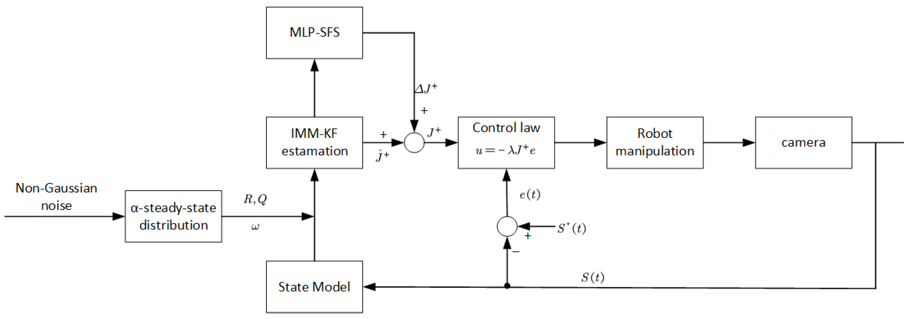
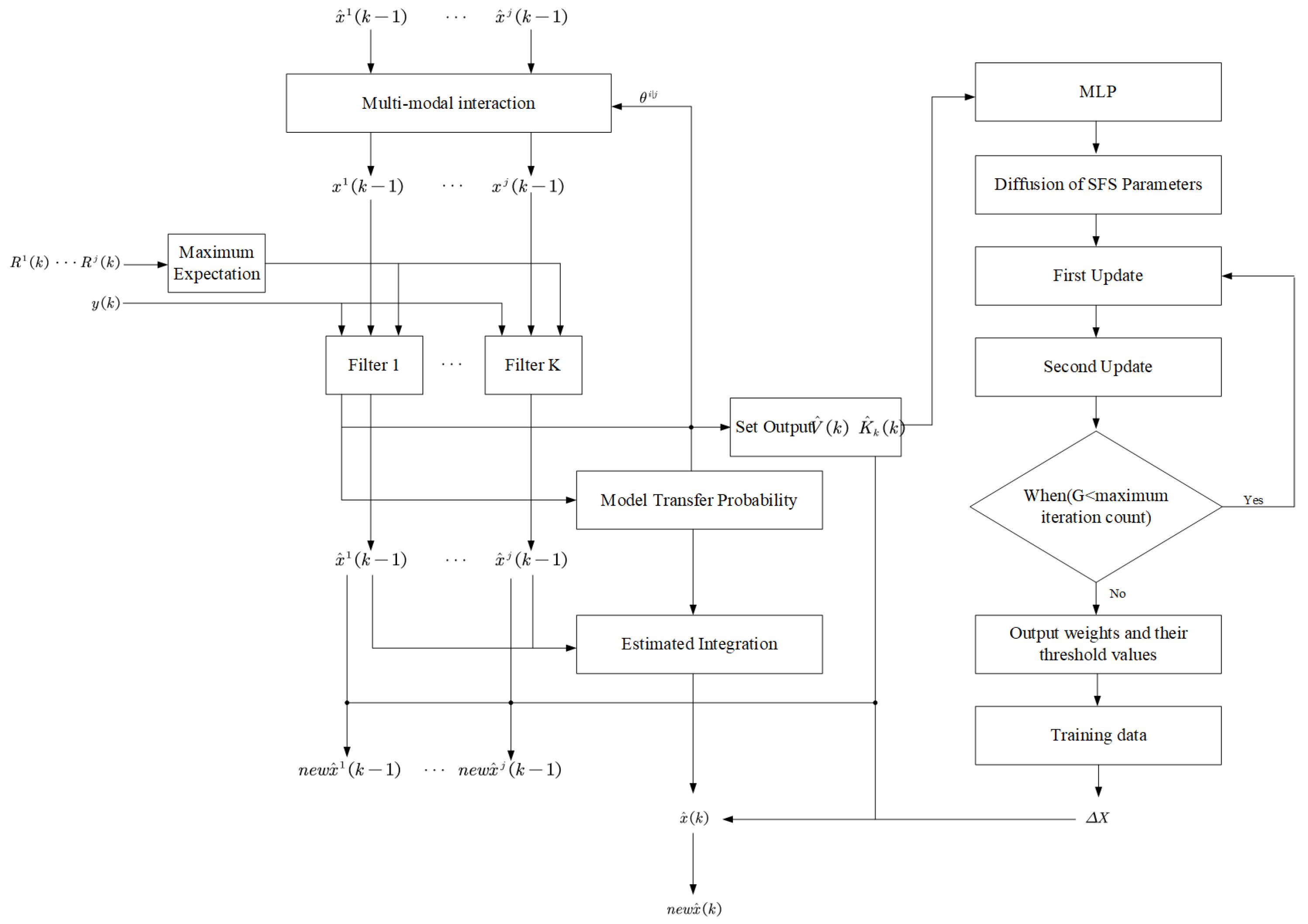
To visually illustrate the data flow and logical interactions among the α -stable distribution modeling, IMM-KF filter, and SFS-MLP compensator, thereby making the entire “intelligent controller” architecture clearly discernible, overall block diagrams have been added. The overall Framework of the IMM-MLP-SFS Algorithm is shown in Figure 1.
The remainder of this paper is organized as follows: Section 2 establishes a noise modeling framework based on the α -stable distribution. Section 3 details a hybrid approach combining IMM with the MLP-SFS compensation mechanism. Subsequently, Section 4 and Section 5 present analytical validation through numerical simulations and experimental studies, respectively. Finally, Section 6 concludes the paper with a summary of key findings and potential research directions.

2. Description of the Problem

2.1. Background

The visual servoing system utilizes the error of the current image feature with respect to the desired feature as a feedback signal to control robotic motion, thereby achieving precise positioning of the end-effector camera. At time step k, the image-space error e ( k ) is defined as
e ( k ) = S ( k ) S * ( k ) ,
where S ( k ) = [ S 1 ( k ) , , S m ( k ) ] T R m denotes the image feature vector at time k, S ˙ ( k ) R m denotes the velocity of the image features, and m is the number of feature points, with S * ( k ) R m being the feature vectors of the desired image. Let r ( k ) = [ r 1 ( k ) , , r m ( k ) ] T R n denote the pose of the robot’s end-effector, and r ˙ ( k ) R n denote the velocity of the robot’s end-effector, where n = 6 . The relationship between r ˙ ( k ) and S ˙ ( k ) can be expressed as follows:
S ˙ ( k ) = J i m a g e ( k ) · r ˙ ( k ) ,
J i m a g e ( k ) = j 11 j 1 n j m 1 j m n m × n ,
where J i m a g e ( k ) denotes the Jacobian matrix of the image.
To move the robot from its current pose to the desired pose, a commonly employed strategy is to utilize a simple linear controller, expressed as
r ˙ ( k ) = λ · J i m a g e + ( k ) · e ( k ) ,
where J i m a g e + ( k ) denotes the pseudoinverse of the image Jacobian matrix, and λ represents the proportionality constant.
Consider the robot visual servoing system described by the following linear discrete equations:
x ( k ) = x ( k 1 ) + w ( k ) , y ( k ) = H x ( k ) + v ( k ) ,
where x ( k ) = [ j 11 , , j m n ] T R ( m × n ) × 1 represents the system’s state vector, x ( k ) is formed by stacking all the elements of the image Jacobian matrix J i m a g e k (Equation (3)) in row-major order. y ( k ) R m denotes the system’s measurement vector, w R ( m × n ) × 1 denotes the process noise, v ( k ) R m denotes the measurement noise, and H R m × m × n denotes the measurement matrix. The structure needs to be determined based on the specific physical relationship between y ( k ) and x ( k ) . In this system model, this relationship stems from the mapping between the image feature changes defined by Equation (2) and the end-effector velocity of the robot.

2.2. Non-Gaussian Noise Modeling Based on α -Steady-State Distribution

The α -stable distribution is often estimated using approximate or numerical methods due to its lack of a closed-form probability density function. Common estimation methods include the characteristic function method (CF), maximum likelihood estimation (MLE), and approximate methods based on mixture models (such as GMM). Although the MLE method has theoretically optimal statistical properties, it is computationally complex and sensitive to initial values; the CF method relies on the form of the distribution’s characteristic function, and its performance is not stable when there are outliers in the noise. In contrast, the GMM method approximates any distribution using a mixture of a finite number of Gaussian distributions, and the EM algorithm has good numerical stability and convergence in parameter estimation, and has good performance in practical systems. Moreover, in the IMM-KF framework adopted in this paper, the noise model needs to provide the mean and covariance in the form. The means and covariance matrices of each Gaussian component output by GMM can be directly used for the multi-model weight update and state prediction of IMM-KF, achieving a natural transition from noise modeling to state estimation.This study posits that the statistical characteristics of non-Gaussian noise are correlated with the system’s intrinsic dynamic patterns. Specifically, the mixing coefficient a reflects the prior probability of noise originating from a specific Gaussian component and can be regarded as the dominant indicator of the current system mode. By normalizing these coefficients, we obtain an initial estimate of the transition probability:
π i j ϖ j , j = 1 K π i j = 1
where ϖ denotes the mixing coefficient of the jth Gaussian component. This heuristic mapping enables the IMM-KF to adaptively adjust model weights based on the statistical properties of observation noise, thereby enhancing robustness against non-Gaussian disturbances. Although the direct correlation between noise statistics and model switching remains approximate, the experimental results in Section 4 and Section 5 demonstrate that this approach significantly improves estimation accuracy and tracking performance compared to traditional methods. Future research will focus on a more rigorous theoretical analysis of the relationship between noise modeling and multi-model transition dynamics. Therefore, this paper selects GMM + EM as the parameter estimation method for the α -stable distribution to achieve efficient and stable modeling of non-Gaussian noise and provide reliable noise statistical information for the subsequent IMM-KF state estimation and MLP-SFS compensation.
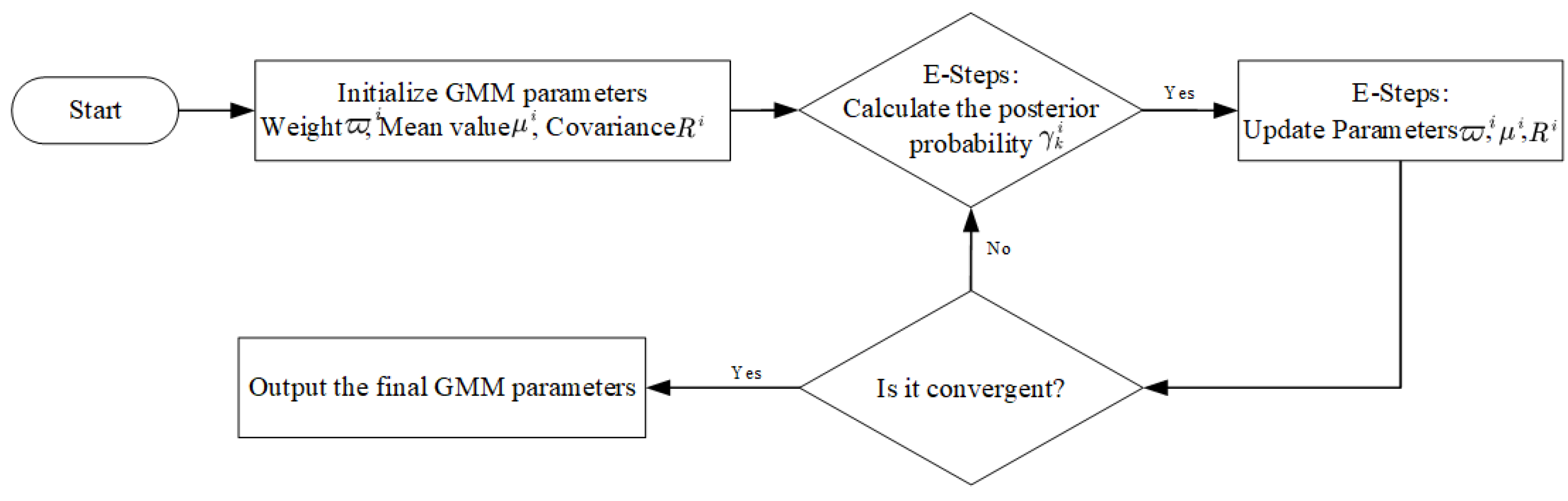
This work employs α -stable distributions to model non-Gaussian measurement noise in visual servoing systems. As such distributions lack analytic probability density functions, a GMM approximation is adopted, with parameters estimated via the Expectation–Maximization algorithm. This approach accurately captures noise characteristics and improves system robustness. The corresponding GMM density function takes the following form:
p ( v k ) = i = 1 k ϖ i f ( v k | μ k i R k i ) , i = 1 k ϖ i = 1 , f ( v k ) = exp { 1 2 [ v k μ k i ] T ( R k i ) 1 [ v k μ k i ] } ( 2 π ) n / 2 R k i 1 / 2 .
In this context, ϖ k i , μ k i , R k i denote probability, mean, and covariance, respectively. The EM algorithm works as follows:
1.
Begin iteration with the initial value of the parameter, t = 0 ;
2.
E-step: Calculate the posterior probability of each sample belonging to each Gaussian distribution, i.e., compute the probability distribution of each sample point within each Gaussian mixture component, as expressed by Equation (8):
γ k i = ϖ t i f ( v k | μ t i , R t i ) k = 1 K ϖ k f ( v k | μ t i , R t i ) .
3.
M-step: Based on the posterior probabilities computed via the E-step, update the mean, variance, and probability of each Gaussian distribution using Equations (9)–(11):
μ t + 1 i = K = 1 N γ k i v k K = 1 N γ k i ,
R t + 1 i = K = 1 N γ k i ( v k μ t i ) ( v k μ t i ) T K = 1 N γ k i ,
ϖ t + 1 i = K = 1 N α k i N .
4.
Repeat the E-step and M-step until convergence.
In this context, noise is defined as general and stationary. We can generate N random samples of noise k = 1 , 2 , , N , i = 1 , 2 , , K , where K is the number of noise samples in the GMM.
The α -stable distribution modeling and GMM approximation flowchart is shown in Figure 2.

2.3. Controller Stability Analysis

In visual servo systems, the stability of the control law u t = r ˙ t = λ · J i m a g e + t · e t is proven using the direct Lyapunov method. Defining the image feature error e t = S t S * t and omitting t for simplicity, according to formula (1), its dynamic equation is
e ˙ = S ˙ = J r ˙ = λ J J + e
Select a positive definite Lyapunov function:
V ( e ) = 1 2 e T e > 0 , e 0 .
Differentiate Equation (13):
V ˙ = e T e ˙ = λ e T ( J J + ) e .
Since J J + is a symmetric positive semidefinite matrix, we have
V ˙ 0 .
Since J has full row rank, J J + = I , and at this point,
V ˙ = λ e T e = 2 λ V < 0 .
The system exhibits global stability.
This stability analysis provides the theoretical foundation for subsequent implementation of IMM-KF state estimation and MLP-SFS error compensation: under ideal conditions of zero noise and precisely known Jacobian matrix, the closed-loop system is stable.

3. IMM-KF with α-Stable Noise Modeling and SFS-Optimized MLP Compensation

3.1. Parameter Selection Rationale

The key hyperparameters of the MLP-SFS compensation module are selected through architectural heuristics, prior experience in the domain, and preliminary experimental tuning. Considering the approximation theorem and the computational efficiency of the control, a single hidden layer MLP structure is adopted. The number of neurons in the hidden layer ( H = 10 ) is initialized with the general heuristic H = m + n + o , where m , n , o represent the input, output, and dimension of the small constant respectively, and is subsequently optimized by cross-validation.The SFS parameters (including population size N = 50 , maximum iteration number I t e r max = 100 and diffusion coefficient 0.5) are selected according to mature metaheuristic design principles and pre-experimental convergence behavior. For the selection of other parameters, the learning rate for updating the weights of the multi-layer perceptron is set to 0.01 to ensure a stable and non-oscillatory convergence process. The convergence threshold of SFS is set to 10 4 . This achieves a reasonable balance between accuracy and computational complexity.

3.2. Robust Estimation Under α -Stable Noise via IMM-KF

IMM-KF is a multi-model target tracking filtering algorithm. Its core mechanism involves dynamically estimating the posterior probability of each model, then using this as a weight to fuse the state predictions from each model, ultimately yielding a more accurate estimate of the target’s state. Equation (6) of the robot visual servoing system is rewritten as follows:
x i ( k ) = x i ( k 1 ) + w ( k ) , y ( k ) = H x i ( k ) + v i ( k ) .
In the IMM-KF algorithm, the transition probability matrix is a crucial parameter. It is defined by the estimated parameters α i from the GMM model, where π i j represents the transition probability from model i to model j.
π i j = α 11 α 1 K α K 1 α K K , i = 1 M π i j = 1 , 0 π i j 1 .
The definition of the initial value is as follows:
θ i ( k 1 ) = α i x ^ i ( k 1 ) = x 0 P i ( k 1 ) = P 0 ,
where θ i ( k 1 ) a denotes the model transition probability at time k 1 . After obtaining the transition probability matrix, the IMM-KF algorithm formula is as follows [36]:
1.
Model interaction:
c ¯ j = i = 1 K π i j θ i ( k 1 ) ,
θ i | j ( k 1 ) = π i j θ i ( k 1 ) c ¯ j ,
x j ( k 1 ) = i = 1 K x ^ i ( k 1 ) θ i | j ( k 1 ) ,
P j ( k 1 ) = i = 1 K θ i | j ( k 1 ) { P i ( k 1 ) + [ x ^ i ( k 1 ) x j ( k 1 ) ] · [ x ^ i ( k 1 ) x j ( k 1 ) ] T } ,
where θ i | j ( k 1 ) is the transition probability from model i to model j, c ¯ j is the prediction probability of model j, x ^ j ( k 1 ) and P j ( k 1 ) denote the state estimate and covariance estimate at time k 1 .
2.
Parallel filtering:
x ^ j ( k | k 1 ) = A x j ( k 1 ) ,
P j ( k | k 1 ) = A P j ( k 1 ) A T + Q ( k ) ,
K k j = P j ( k | k 1 ) H T H P j ( k | k 1 ) H T + R j ( k ) ,
x ^ j ( k ) = x j ( k | k 1 ) + K k j ( y ( k ) H x ^ j ( k | k 1 ) ) ,
P j ( k ) = ( I K k j H ) P j ( k | k 1 ) ,
F j ( k ) = H P j ( k | k 1 ) H T + R j ( k ) ,
V j ( k ) = y ( k ) H x ^ j ( k | k 1 ) .
3.
Model probability updates:
L j ( k ) = c ¯ j ( 2 π ) n / 2 | F k j | 1 / 2 exp ( 1 2 ( V k j ) T F k j ( V k j ) ) ,
c ( k ) = j = 1 K c j ( k ) c ¯ j ,
θ j ( k ) = L j ( k ) c ¯ j c ( k ) .
4.
Estimation fusion:
x ^ ( k ) = j = 1 K x ^ j ( k ) θ j ( k ) ,
P ( k ) = i = 1 K θ j ( k 1 ) { P j ( k ) + [ x ^ j ( k ) x ^ ( k ) ] · [ x ^ j ( k ) x ^ ( k ) ] T } .

3.3. Accuracy Compensation Strategy for MLP Based on SFS Technology

During image Jacobian matrix estimation using IMM, two critical errors emerge: model inaccuracy and noise interference. To address these limitations, this section introduces a hybrid MLP-SFS compensation mechanism that enhances estimation accuracy under non-Gaussian noise conditions.
  • Measurement noise and Kalman gain from Equations (36) and (37) are fed as input to the MLP-SFS algorithm.
    V ^ ( k ) = j = 1 K V j ( k ) θ j ( k ) ,
    K ^ k ( k ) = j = 1 K K k j ( k ) θ j ( k ) .
  • Initialization of SFS and MLP parameters, including population size, upper and lower bounds, number of neurons in hidden layers, lateral walk, and maximum diffusion number.
  • Matrix Encoding Strategy
    Concatenate the fusion values V ^ k of the measurement noise and the fusion values K ^ k k of the Kalman gain in chronological order to form the input matrix G k , which serves as the input to the MLP-SFS:
    G ( k ) = V ^ ( 1 ) V ^ ( k ) K ^ k ( 1 ) K ^ k ( k ) .
    This input simultaneously incorporates the statistical characteristics of the system’s observational noise and the historical information of the filtering gain, which is helpful for the MLP to learn the dynamic pattern of the estimation error.
    Based on the given input samples and output targets, the network structure of the MLP is determined. This paper adopts a 49-10-6 structure for design, and its encoding strategy can be expressed as
    w = w 1 , 1 w 1 , 10 w 1 , 10 w 49 , 10 , b = b 1 b 10 , v = v 1 , 1 v 6 , 1 v 10 , 1 v 10 , 6 , d = d 1 d 6 ,
    where w represents the input weight matrix of the hidden layer, b represents the bias matrix of the hidden layer, v represents the output weight matrix of the hidden layer, and d represents the output layer bias matrix.
    The hidden layer input l j and output o j are as follows:
    l j = i = 1 n w i j G ( k ) b j .
    o j = f ( i = 1 n w i j G ( k ) b j ) ,
    where f ( x ) denotes the sigmoid function.
    The output results for model error and noise error are shown in Equation (43):
    f ( x ) = 1 1 + exp ( x ) .
    Δ X ( k ) = g ( j = 1 m v i j o j d i ) ,
    MLP employs a single hidden layer structure, with the hidden layer containing neurons. The input layer has nodes (corresponding to the dimension of), and the output layer has nodes (corresponding to the dimension of the state vector). The hidden layer uses the sigmoid activation function, while the output layer uses a linear activation function. The training data consists of historical estimation errors from simulations and their corresponding noise sequences. The loss function employs mean squared error (MSE), with the training objective being to minimize the gap between the predicted compensation value and the actual error.
    Based on the idea of error decomposition, the estimation error of IMM-KF can be regarded as two parts: model mismatch and noise interference. By learning the historical noise and gain information, MLP outputs the prediction compensation value Δ x k of the current time estimation error. The compensation term is assigned to the predicted value of each filter according to the posterior probability θ j k of each model:
    In the equation, g ( x ) is a linear function.
    Δ X ( k ) = Δ X mod ( k ) + Δ X n o s i e ( k ) ,
    Δ X j ( k ) = Δ X ( k ) θ j ( k ) ,
    Δ X ¯ ( k ) = x ( k ) x ^ ( k ) ,
    where Δ X represents the output after optimizing the weights in the MLP-SFS, which incorporates the model error Δ X mod ( k ) and noise error Δ X n o i s e ( k ) , Δ X i ( k ) denotes the accuracy compensation for the prediction value of the j-th parallel filter in the IMM-KF, where j = 1 K and Δ X ¯ represent the error between the true value and the predicted value. x ( k ) is the true value, and Δ x ^ ( k ) is the predicted value.
    Then, use MSE to evaluate the accuracy of the predicted values relative to the actual values, with the formula as follows:
    M S E = 1 n ( Δ X ( k ) Δ X ¯ ( k ) ) .
    The fusion method is essentially an error correction strategy based on posterior probability weighting, and its effectiveness has been verified in the framework of Bayesian estimation [37].
    Here, Δ X represents the output after optimizing the weights in the MLP-SFS, Δ X j ( k ) denotes the accuracy compensation for the prediction value of the j-th parallel filter in the IMM-KF, where j = 1 K and Δ X ¯ represent the error of the true value relative to the predicted value. x ( k ) is the true value, and Δ x ^ ( k ) is the predicted value. Then, the accuracy of the predicted values is evaluated relative to the actual values using MSE.
  • Diffusion process
    At each iteration before convergence, the MLP’s parameters (weights and thresholds) diffuse from their current positions using Gaussian sampling. This diffusion mechanism enables comprehensive exploration of the search space to identify optimal parameter configurations.
    G W 1 = G a u s s i a n ( μ B P , σ ) + ( ε × B P ε × P i ) ,
    G W 2 = G a u s s i a n ( μ P , σ ) ,
    σ = log ( g ) g × ( P i B P ) ,
    where ε and ε are random numbers uniformly distributed over [ 0 , 1 ] , B P is the optimal point, P i is the point at the i-th position, and μ B P and μ P are equivalent to B P and P i .
  • Sorting
    During diffusion, parameters (weights and thresholds) are probabilistically screened, with top-ranked candidates selected for the search space. Following initialization, a merit-based ranking is applied to refine parameter sets, systematically improving the probability of converging to the global optimum.
    P a i = r a n k ( P i ) N ,
    where P a i denotes all parameters, while denotes the number N of all parameters, r a n k ( P i ) indicates the position of P i after sorting the data in ascending order.
  • Update Process
    After all weights and thresholds are sorted, these values undergo a first update and are reordered based on the output error of the fitness function. The second update aims to enhance the quality of the search space and satisfy diversity requirements.
    First Update
    P i = P r ( j ) ε × ( P t ( j ) P i ( j ) ) .
    Second Update
    P i = P i ε × ( P t B P ) ε 0 . 5 ,
    P i = P i ε × ( P t P r ) ε > 0 . 5 .
    Points P t and P r are randomly selected from the points chosen in the first update [38].
  • Terminate training of the multilayer perceptron
    The training process terminates when the mean squared error (MSE) of the objective function converges or shows negligible improvement over successive iterations. Otherwise, the algorithm returns to step (1).
Upon convergence, the optimized weights and thresholds are used to train the input samples. The resulting compensated estimates are then integrated into the IMM framework. The final optimized state estimate of the image Jacobian matrix is denoted as n e w x ^ ( k ) = Δ X ( k ) + x ^ ( k ) .
The workflow based on the IMM-MLP-SFS algorithm is shown in Figure 3.

4. Numerical Simulation and Analysis

This section presents simulation studies performed on a 6-DOF robotic manipulator equipped with an end-effector camera. A static target comprising four circular feature points is used to evaluate the system. The robot executes visual servoing tasks under two distinct operating conditions, demonstrating the robustness and effectiveness of the proposed method.

4.1. Simulation Case 1: Performance Validation of the IMM-MLP-SFS Algorithm

The camera’s focal length measurement is 8 mm, the recorded image size is 800 × 800 , λ = 0.5 , the convergence threshold is set to 0.5. The specific noise settings are as follows: Pulse noise is a mixture of salt noise and pepper noise, with occurrence probabilities of P s a l t = 0.05 and P p e p p e r = 0.05 respectively. The noise amplitudes are set to 255 and 0 respectively. Additionally, the noise covariance was set to R = 1 × 10 5 × I 8 × 8 to simulate the actual sensor noise environment. The process noise covariance matrix Q reflects the uncertainty in the system model. In this simulation, Q is set to 4 × 10 2 × I 48 × 48 . This value is determined based on error analysis of the robot’s kinematic model and prior experimental data, aiming to reasonably simulate random disturbances during joint motion. The robot’s initial joint position is q 1 = [ 0 , π / 2 , 0.8 × π , 0 π / 4 , π / 4 ] , and the desired image feature is S * ( k ) = 400 200 200 400 400 400 600 600 . The state transition probability is π i j = 0.1 0.9 0.1 0.9 .
In the simulation experiments, all algorithms under comparison (such as KF, IMM, MCKF, etc.) underwent parameter optimization and were tuned to their optimal states. The optimization process employed grid search and cross-validation methods, with minimizing tracking error as the objective function. All algorithms operated under identical non-Gaussian noise conditions.
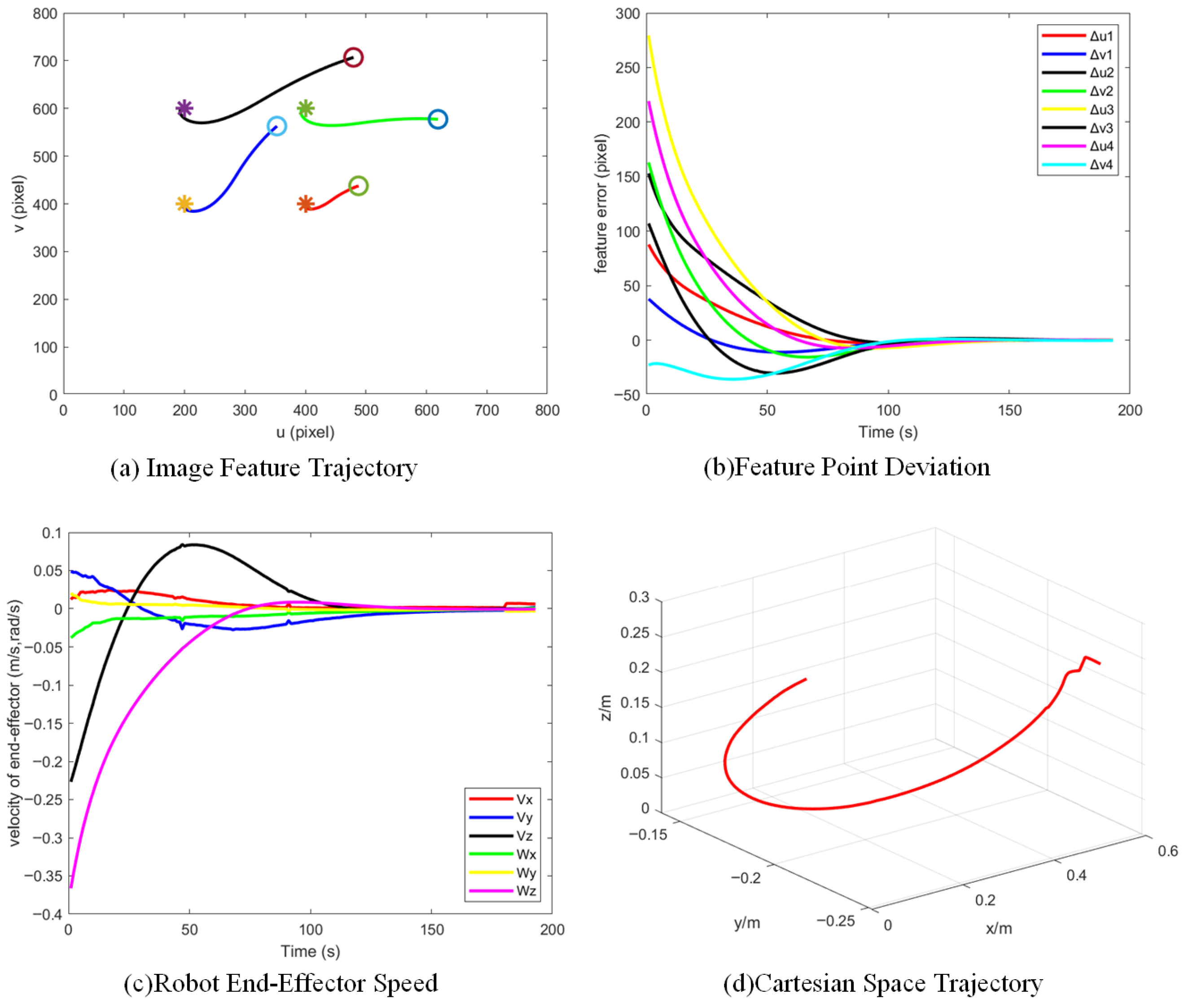
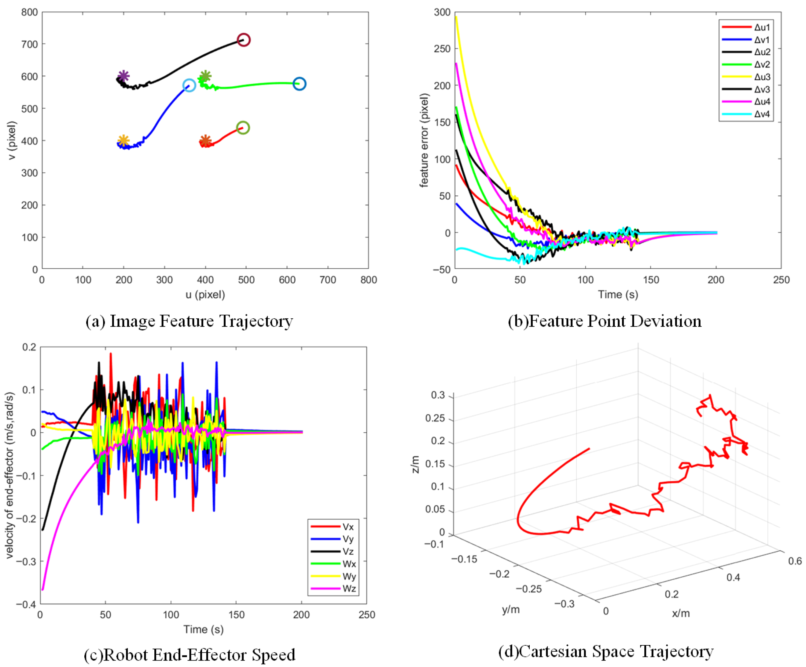
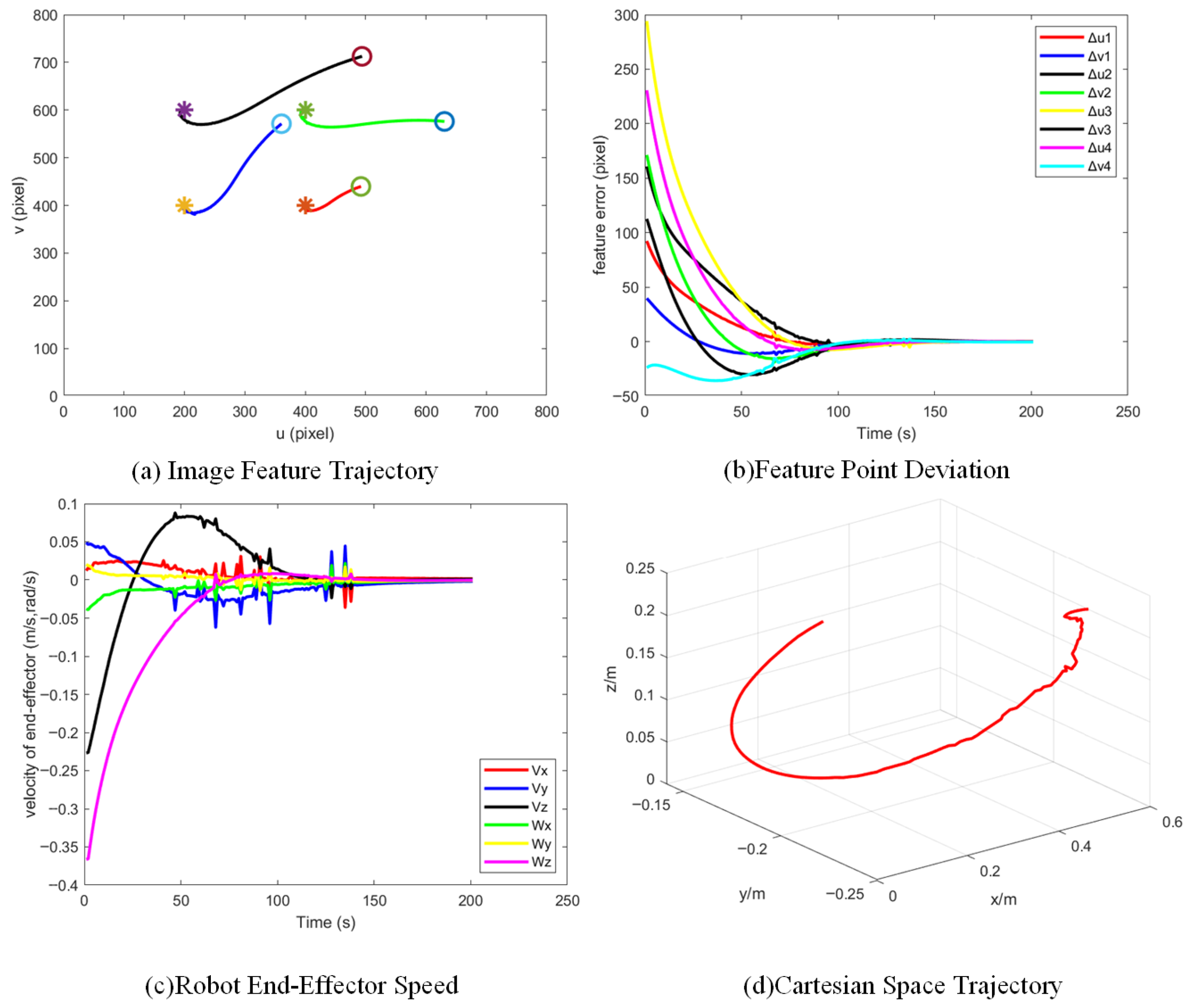
This study evaluates the robustness of the proposed IMM-MLP-SFS method for Jacobian matrix estimation through a comparative analysis with the conventional KF and standard IMM algorithms. Figure 4, Figure 5 and Figure 6 present a comparative analysis of the positioning control performance achieved by three distinct algorithms operating under identical non-Gaussian noise conditions in a visual servoing system. As illustrated in Figure 4a,d, the standard KF demonstrates limited robustness in such environments. The image feature trajectory exhibits significant oscillatory behavior during convergence, preventing the tracking error from stabilizing at the target setpoint. Furthermore, the velocity profile of the end-effector camera shows substantial fluctuations between iterations 40 and 140, resulting in pronounced irregularity in the robot’s Cartesian motion trajectory. To mitigate these issues, the IMM algorithm was implemented. As depicted in Figure 5, the IMM strategy yields notable improvements over the baseline KF in both image-space tracking and Cartesian motion smoothness. Nevertheless, as evidenced in Figure 5b,c, the mean squared error of feature tracking remains above 0.05 pixels, and the end-effector velocity continues to be perturbed by residual noise, indicating persistent limitations in estimation accuracy. Building on the IMM framework, a compensated approach incorporating an MLP-SFS was introduced. The results in Figure 6 reveal a marked enhancement in performance: the image feature trajectory converges more smoothly and rapidly toward the reference values, with terminal motion oscillations significantly attenuated. Moreover, the Cartesian trajectory exhibits superior smoothness, underscoring the efficacy of the MLP-SFS module in suppressing noise-induced deviations and improving both transient and steady-state behavior.
In summary, the integration of MLP-SFS compensation effectively addresses the key limitations of both the KF and IMM algorithms under non-Gaussian noise, leading to substantial gains in positioning accuracy and motion stability in vision-based robotic control.

4.2. Simulation Case 2: Comparative Simulation of Different Algorithms

This section validates the estimation performance of the image Jacobian matrix based on the IMM-MLP-SFS method by comparing it with the SVSF-KF, MCKF, and ARKF methods. In the simulations, the robot’s initial position is denoted as q 2 = [ 0 , π / 4 , π , 0 , π / 4 , π / 4 ] .
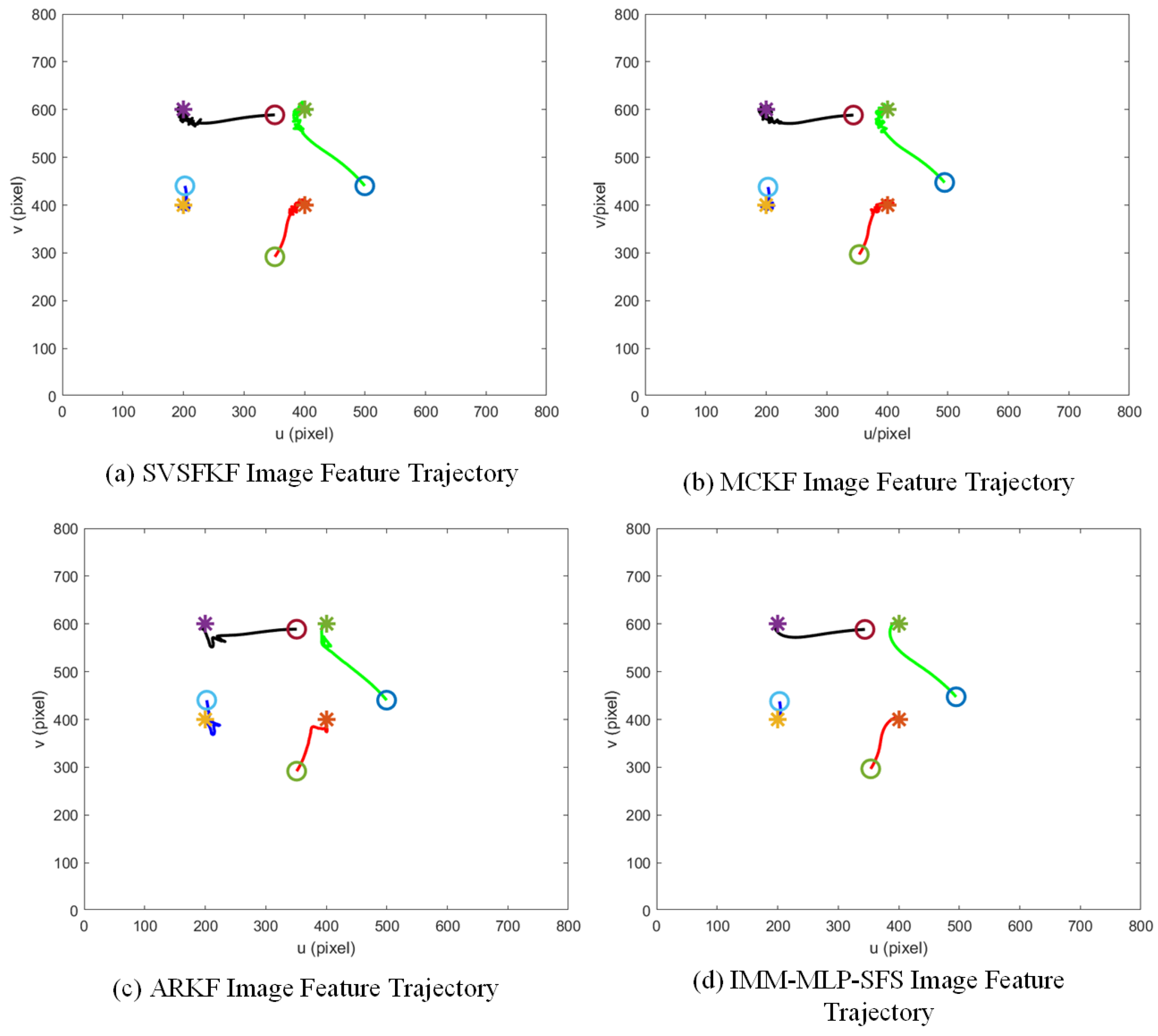
Figure 7 compares the trajectories of image feature points under impulse noise conditions for four different algorithms.The ARKF algorithm fails to achieve stable localization, with its feature trajectory displaying substantial oscillatory behavior near the target and an inability to converge smoothly. Performance improves with the MCKF algorithm, which yields a relatively smoother trajectory and reduced fluctuations; nevertheless, considerable jitter persists during the final approach to the target. The SVSF-KF algorithm further refines trajectory behavior, though it still exhibits pronounced and, at times, more severe jitter in the target region. In contrast, the proposed IMM-MLP-SFS algorithm achieves the smoothest and most stable trajectory, with no observable oscillations near the target, demonstrating a clear advantage in both accuracy and disturbance rejection.
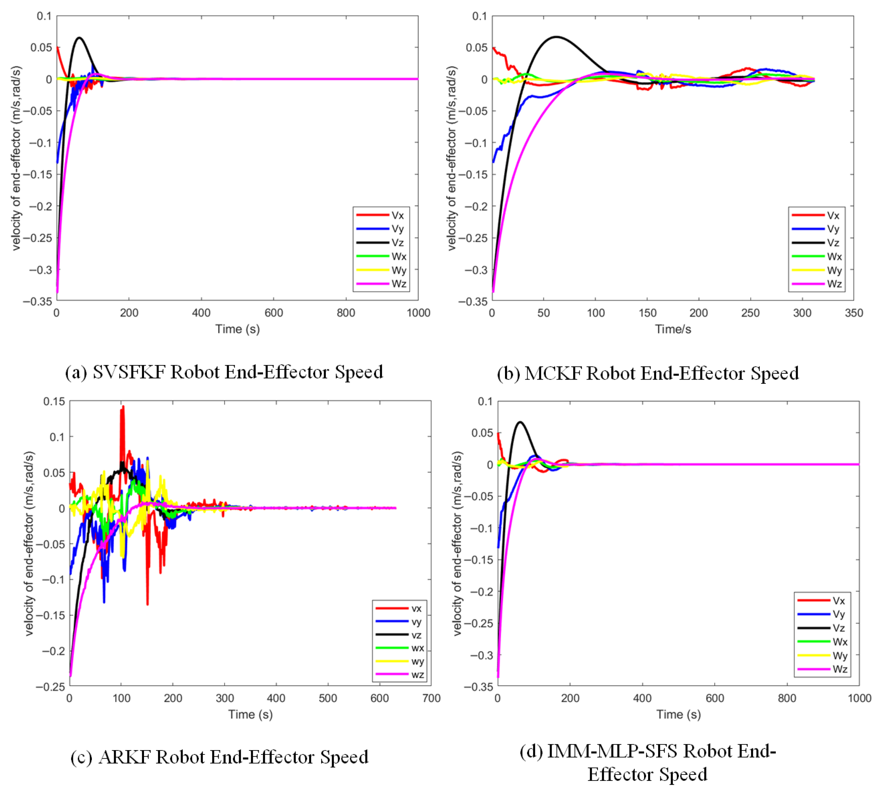
To more effectively illustrate different performance dimensions, Figure 8 and Figure 9 employ distinct time scales on their horizontal axes. Figure 8 demonstrates error convergence throughout the entire task cycle, while Figure 8 focuses on velocity response during the initial transient phase. Both perspectives indicate that the proposed IMM-MLP-SFS method exhibits the fastest convergence rate and optimal stability.
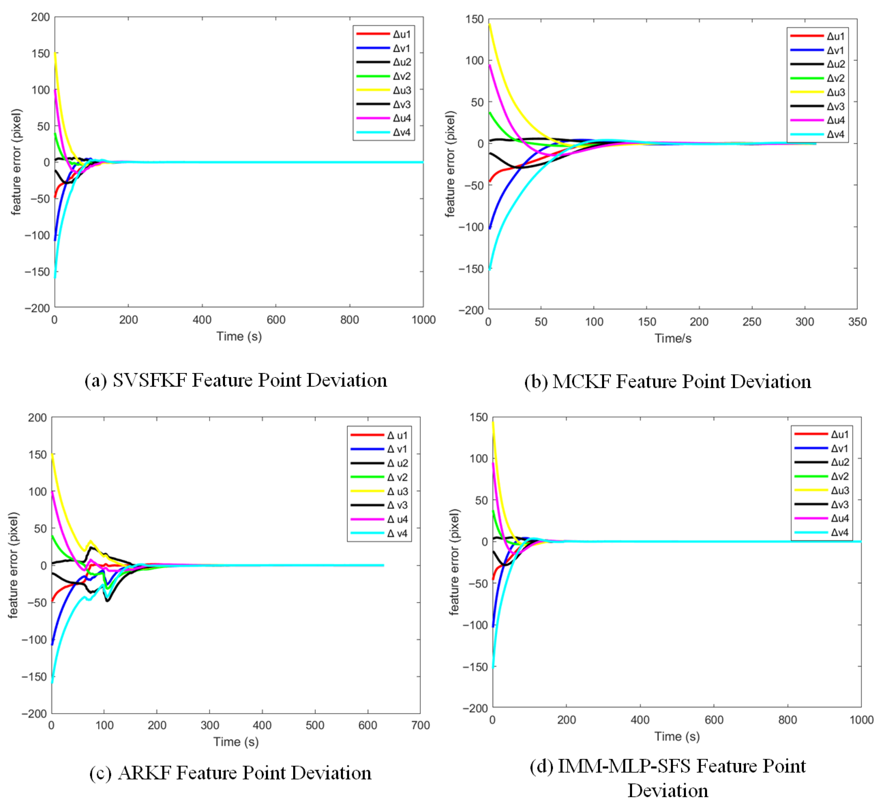
Tracking errors of the four algorithms are shown in Figure 8. Under the influence of non-Gaussian noise, the ARKF algorithm exhibits a diverging error trend, indicating inadequate robustness in such conditions. The MCKF algorithm attains error convergence with greater stability than ARKF, yet continues to display fluctuations as the error approaches zero, limiting final accuracy. Although the SVSF-KF algorithm converges more rapidly, it does not fully suppress error variations near the target. By comparison, the IMM-MLP-SFS algorithm achieves the fastest convergence and maintains the smallest error fluctuations, underscoring its superior stability and precision.
Velocity profiles in Figure 9 further highlight control performance differences. The ARKF algorithm shows severe velocity fluctuations, reflecting significant sensitivity to non-Gaussian noise. While the MCKF algorithm reduces such fluctuations to some extent, it still permits residual jitter. The SVSF-KF algorithm delivers a generally smoother velocity response with reduced noise impact, though minor oscillations remain near the target. The proposed IMM-MLP-SFS method, however, produces the smoothest velocity profile, with negligible influence from noise and excellent overall stability.
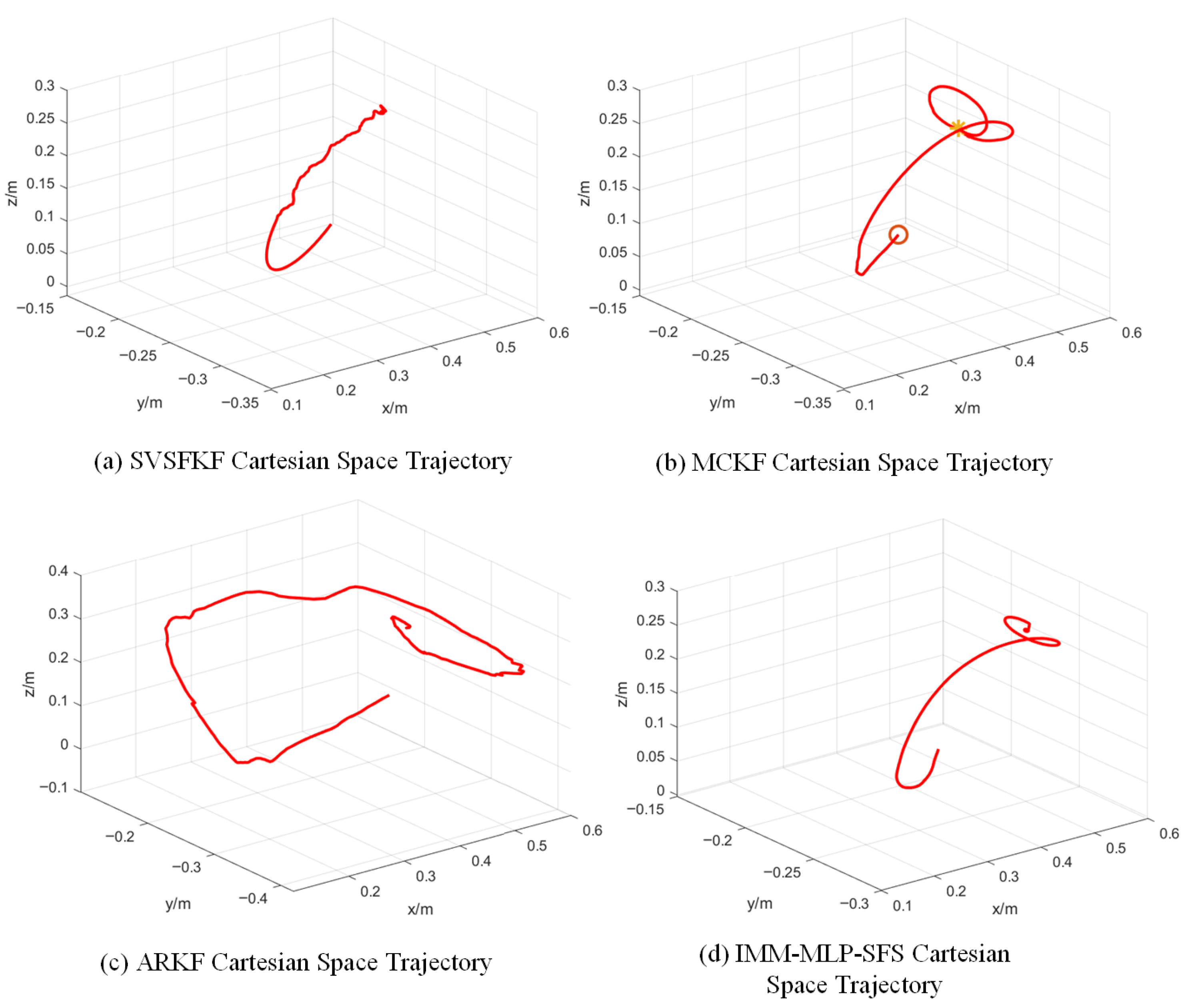
As illustrated in Figure 10, Cartesian-space tracking performance aligns with the above trends. The ARKF algorithm results in large fluctuations at the end-effector level and fails to track the reference path effectively. The MCKF algorithm improves trajectory smoothness but does not eliminate terminal jitter. The SVSF-KF algorithm yields relatively stable motion yet shows more pronounced jitter near the target compared to the others. The IMM-MLP-SFS algorithm again outperforms the others, generating the smoothest Cartesian trajectories with no significant jitter during the approach.
In summary, the proposed IMM-MLP-SFS algorithm demonstrates consistent superiority across all evaluation metrics image feature tracking, error convergence, velocity regulation, and end-effector trajectory smoothness. By effectively mitigating the impact of non-Gaussian noise, the method significantly enhances the positioning accuracy, robustness, and overall performance of the visual servoing system, enabling more reliable and precise task execution.
The experimental results demonstrate that the IMM-MLP-SFS algorithm consistently outperforms conventional methods across all evaluation metrics, including trajectory tracking, error convergence, velocity regulation, and Cartesian-space motion smoothness. This method effectively suppresses interference from non-Gaussian noise, significantly enhancing the system’s positioning accuracy. Simultaneously, it strengthens the overall stability and robustness of the system. This further demonstrates the practical potential of vision servoing systems in demanding industrial environments.
The performance metrics of different methods in the simulation diagram above are shown in Table 1.

4.3. Simulation Case 3: Application Scope and Generalization Capability of the IMM-MLP-SFS Algorithm

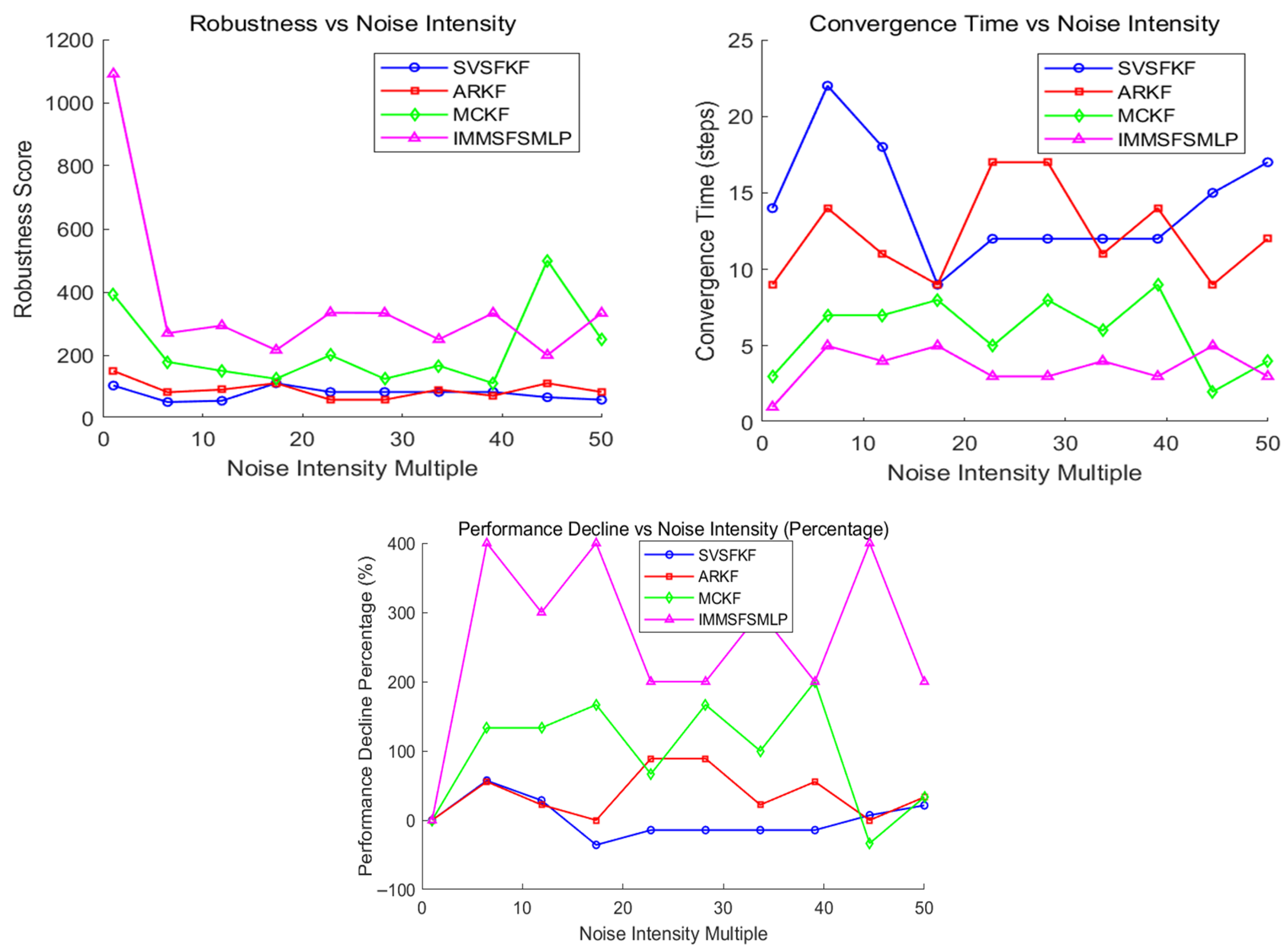
This paper extends the application scope of the IMM-MLP-SFS algorithm under strong impulse noise conditions. Simple settings for noise intensity and duration ratio are defined: noise intensity is scaled from 1 to 50 times, and duration ratio ranges from 10 % to 50 % . The generalization capability of the SFS component within the IMM-MLP-SFS algorithm is also evaluated.
Figure 11 illustrates the robustness, convergence time, and performance degradation of various algorithms under different noise intensities. At a 6.4-fold noise intensity, the robustness and performance of the IMM-MLP-SFS algorithm significantly deteriorate, yet its overall robustness remains superior to other algorithms. Regardless of noise intensity, this algorithm’s convergence time consistently outperforms that of other methods. This indicates that the IMM-MLP-SFS algorithm remains applicable even under more extreme conditions.
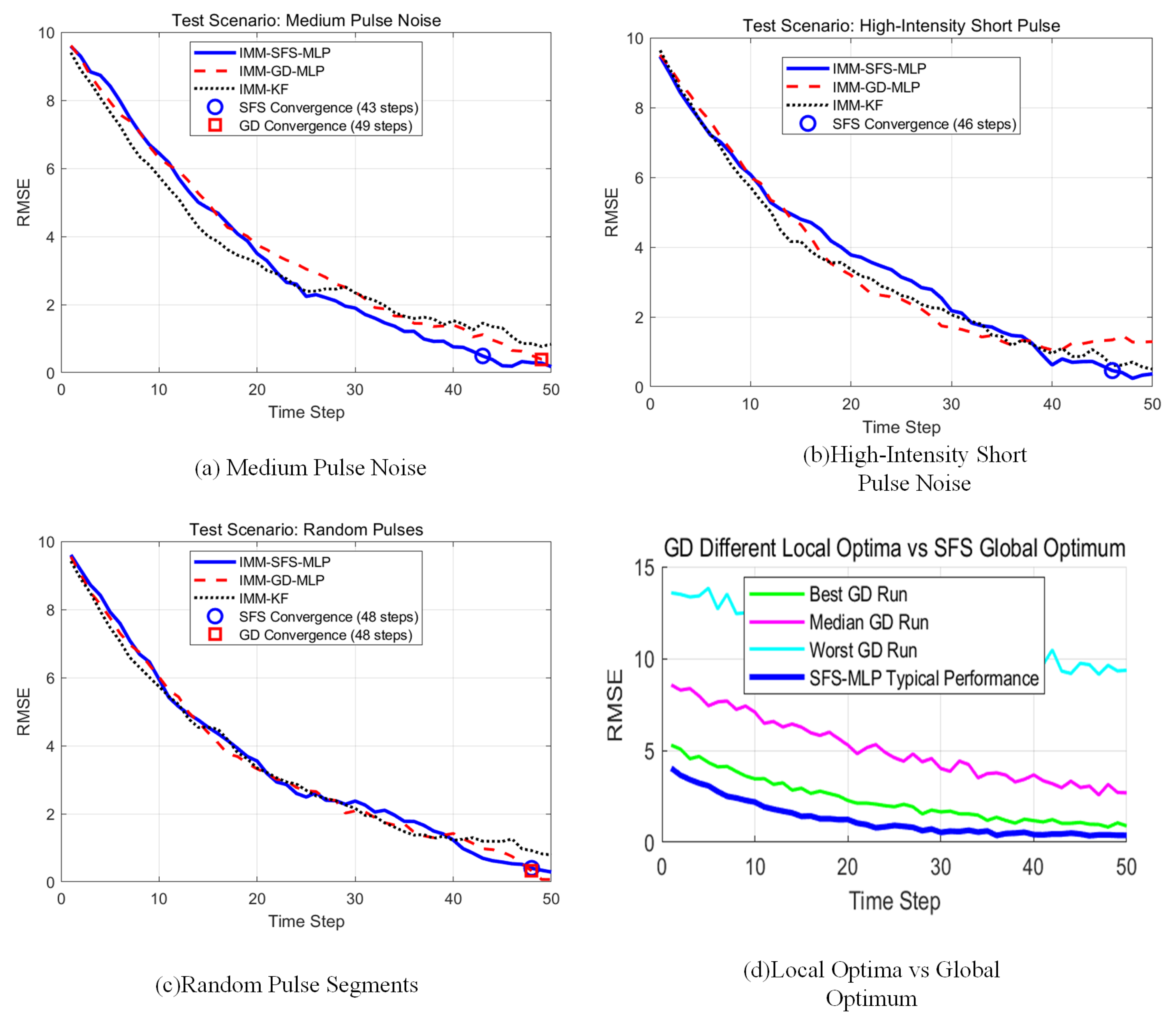
Figure 12a shows that the three algorithms exhibit similar estimation accuracy. However, during convergence, IMM-MLP-SFS converged at step 43, while IMM-MLP-GD did not converge until step 49, indicating a risk of getting stuck in local optima. Therefore, under moderate noise conditions, the IMM-MLP-SFS algorithm converges faster and achieves global optimality. Figure 12b features high noise intensity and short duration, demanding robust and adaptive algorithms. The IMM-MLP-SFS algorithm significantly outperforms the other two, demonstrating strong robustness and recovery capability. In Figure 12c, both IMM-MLP-SFS and IMM-MLP-GD exhibit identical convergence speeds under random noise. Figure 12d further highlights the global optimal performance of the IMM-MLP-SFS algorithm. Therefore, IMM-MLP-SFS outperforms both the IMM-MLP-GD and IMM-KF methods in terms of convergence speed, robustness against sudden noise, and global optimization capability.

5. Experimental Verification

5.1. Experimental Platform and Disturbance Configuration

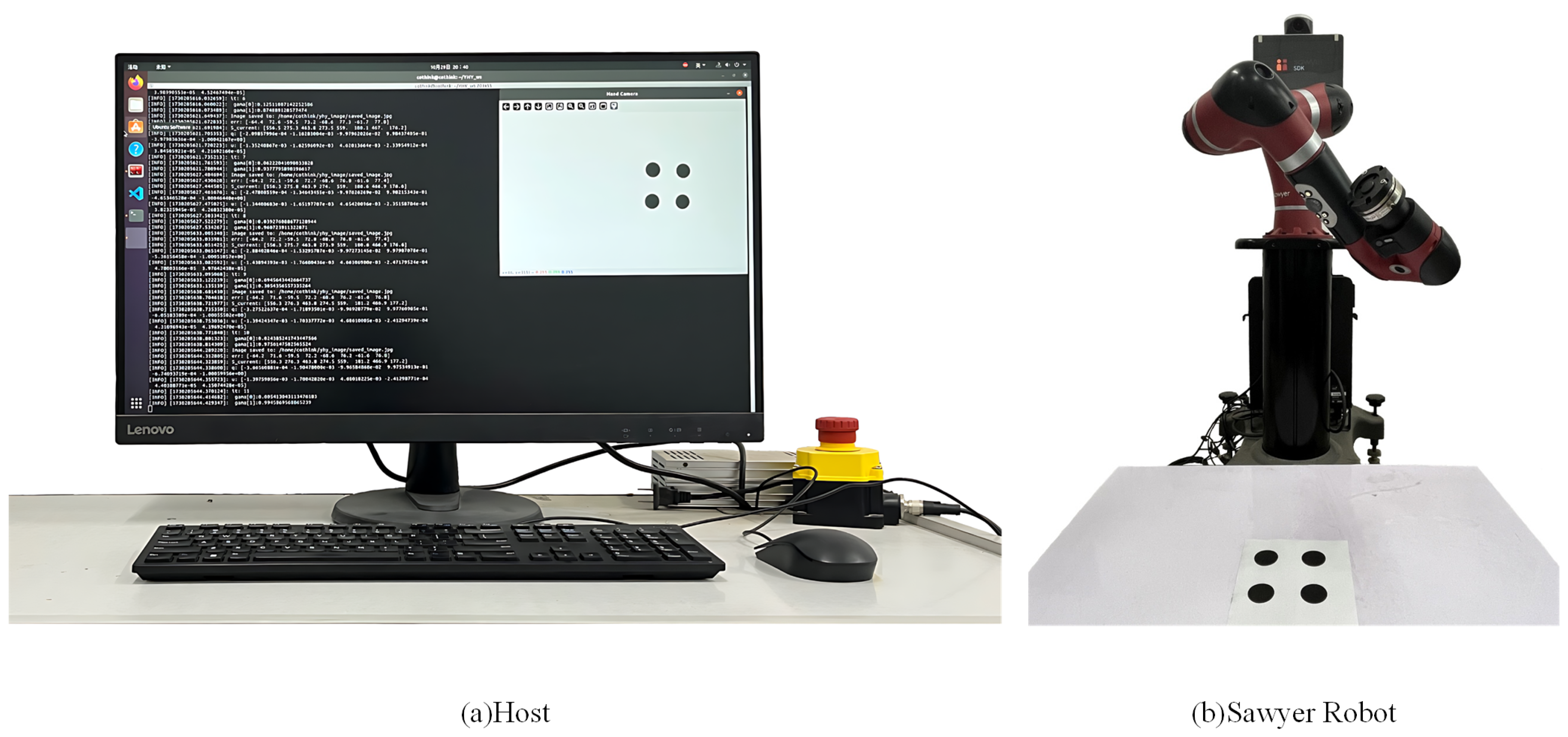
The robot platform of the Sawyer cooperative robot manipulator was used for the experiments. In this study, only the first six rotary joints are actuated, and the seventh joint remains fixed to form a six-degree-of-freedom (DOF) system, as shown in Figure 13. The native Intera5.1.0 software suite and ROS driver were used to control the robot, and the joint position and velocity commands were realized at the control frequency of 100 Hz. The workspace and kinematic limits of the Sawyer manipulator define the operational constraints of the visual servoing task.
A Cognex ISC-1501C industrial camera manufactured by Cognex Corporation in Natick, MA, USA, (resolution 752 × 480 ) was rigidly mounted on the wrist (end-effector) of the robot to constitute the vision sensor configuration in eye–hand mode. The camera is connected to the host PC through the GigE interface. Before the experiment, the OpenCV standard checkerboard calibration process was used to obtain its internal reference matrix K. No external calibration between the camera and the end-effector was performed, conforming to the “uncalibrated” visual servoing paradigm. Image acquisition and processing were run at about 20 Hz within the ROS node. The proposed algorithm and the comparison method were implemented in Python 3.8. The host was configured with an Intel Core i7-4770s processor and 8 GB RAM. The communication between the algorithm, ROS, and Sawyer SDK was implemented through the API interface.
K i n = 626.138 0.0 361.013 0.0 624.880981 216.164993 0.0 0.0 1.0
To simulate real industrial noise environments, noise interference was systematically introduced in the experiment: pulse (salt-and-pepper) noise was generated by simulating sensor failures or transmission errors.
The above interferences together constitute heavy-tailed non-Gaussian noise, and the proposed IMM-MLP-SFS framework is designed to mitigate such noise. The performance of all compared algorithms is evaluated under the same interference condition.
Throughout the entire experimental process, images were captured every 5 s using a wrist-mounted camera. Each image underwent edge detection, exposure adjustment, and proportional gain adjustment via the ROS framework. The visual processing workflow primarily focused on feature point detection and extraction for motion control. In all trials, the proportional gain was set to 0.125, with a convergence threshold of 0.8.

5.2. Accuracy Compensation Experiment

Visual servoing performance is evaluated through a task starting from initial joint angles q 3 = [ 0.0 , 0.0 , 0.0 , 1.55 , 1.6 , 1.5 ] , where image features are first recorded, followed by controlled motion to desired feature S d 1 = [ 417.7 , 311.8 ; 429.3 , 321.2 ; 187.8 , 179.7 ; 80.0 , 68.6 ] .
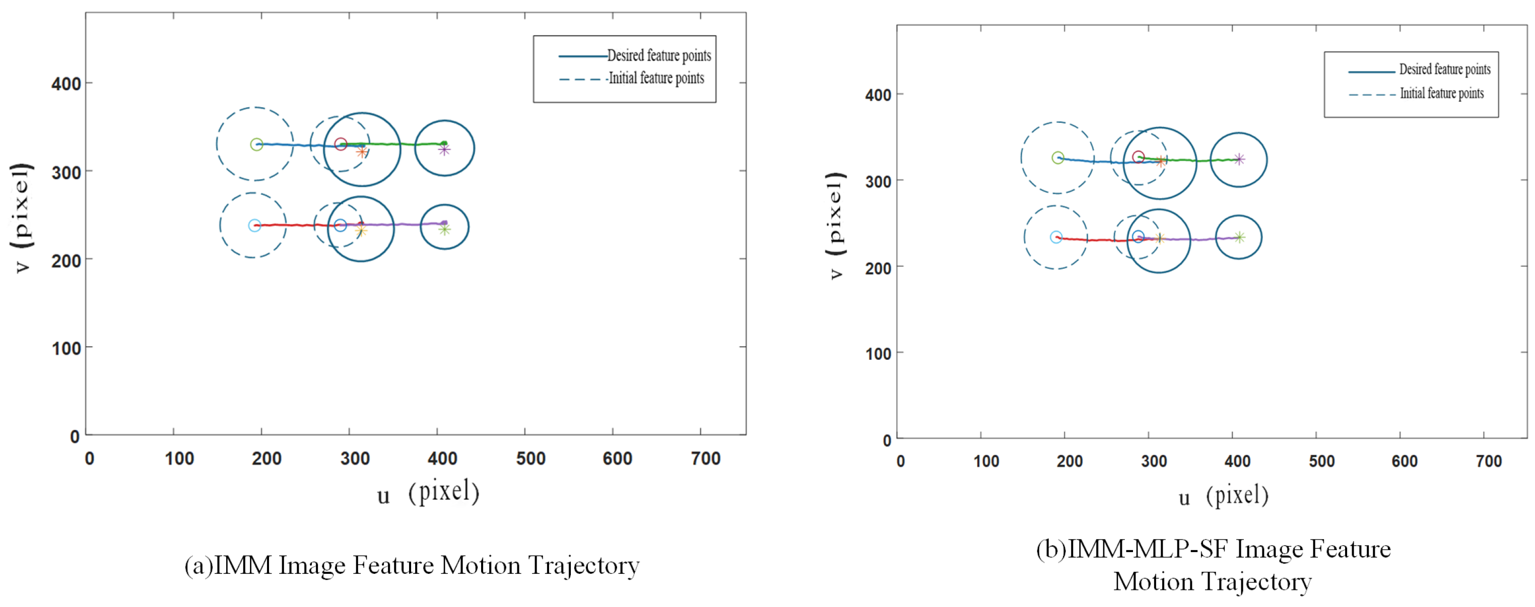
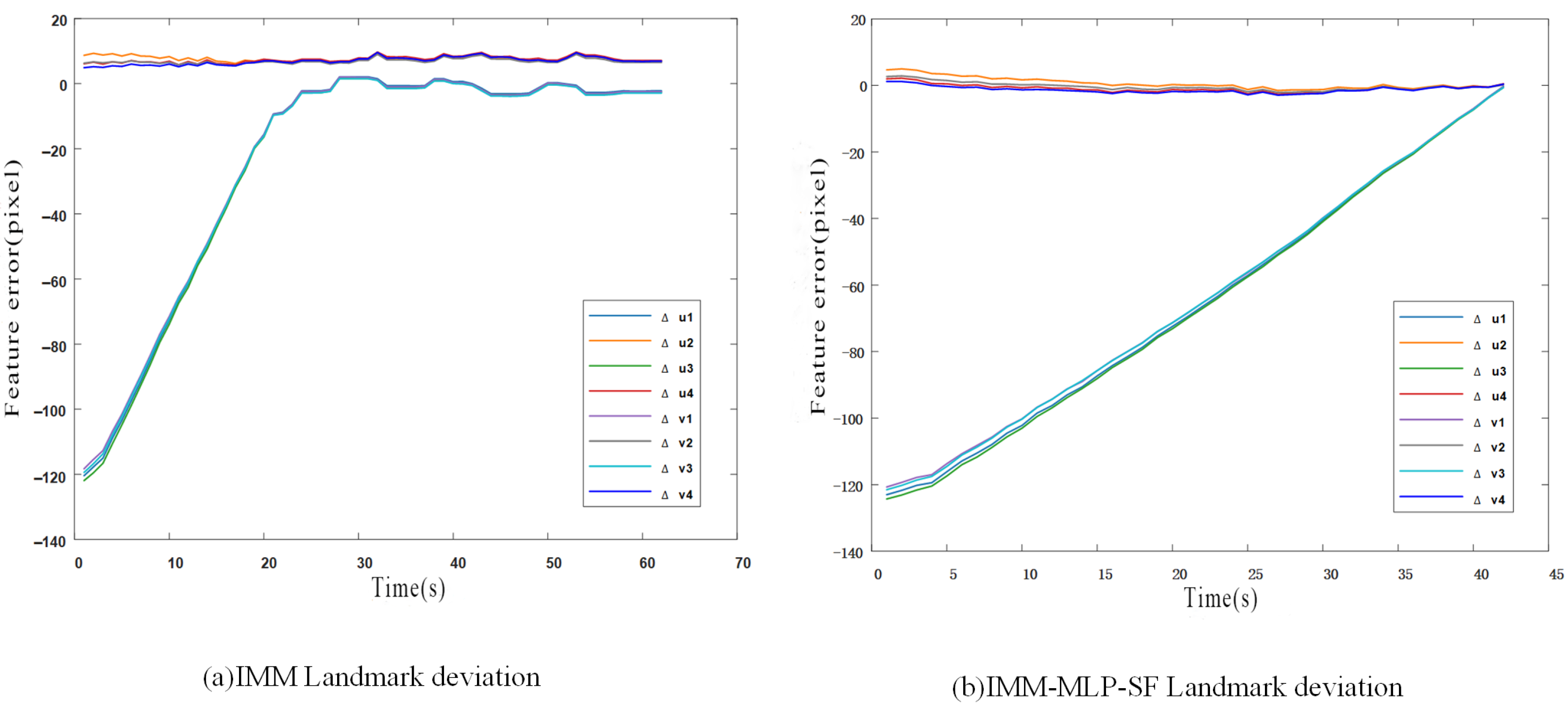
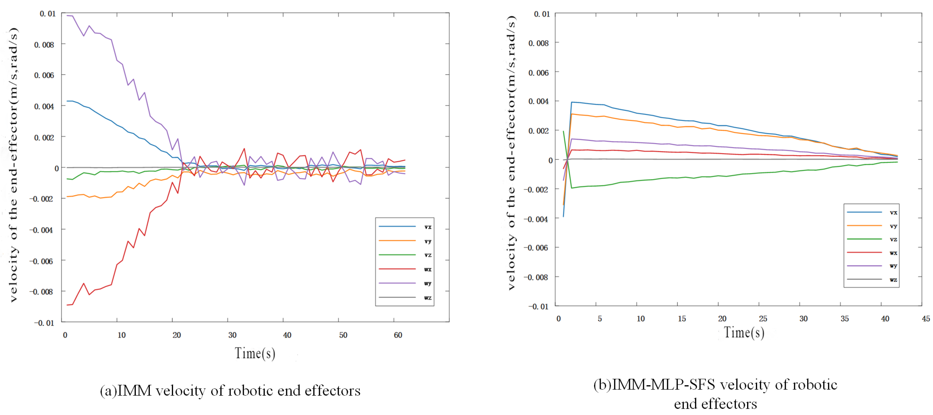
As demonstrated in Figure 14, the IMM algorithm failed to guide the robot within the prescribed image feature threshold during positioning tasks, exhibiting substantial tracking inaccuracies. In contrast, the proposed IMM-MLP-SFS algorithm successfully maintained tracking alignment with the target features, constraining the feature deviation norm within 0.8 pixels. The conventional IMM approach recorded a maximum feature deviation of 8 pixels, and its error convergence stagnated after 20 s of operation, indicating entrapment in a local minimum. Conversely, the IMM-MLP-SFS method achieved rapid convergence to the predefined threshold, as evidenced in Figure 15. The velocity analysis presented in Figure 16a reveals that under non-Gaussian noise conditions, the end-effector velocity controlled by the IMM algorithm developed sustained oscillations, preventing the system from attaining the required positioning precision. Under identical experimental conditions, the IMM-MLP-SFS algorithm demonstrated significantly suppressed vibration levels, enabling stable convergence to the target configuration.

5.3. Performance Comparative Experiment

Experimental validation compares the conventional KF with the proposed IMM-MLP-SFS framework under non-Gaussian noise conditions. The robotic system executes servoing tasks from initial joint angles q 4 = [ 0.0 , 0.0 , 0.1 , 1.0 , 0.0 , 1.0 ] to target feature S d 2 = [ 429.1 , 404.3 ; 490.4 , 405.3 ; 347.9 , 346.7 ; 257.4 , 254.0 ] pixels.
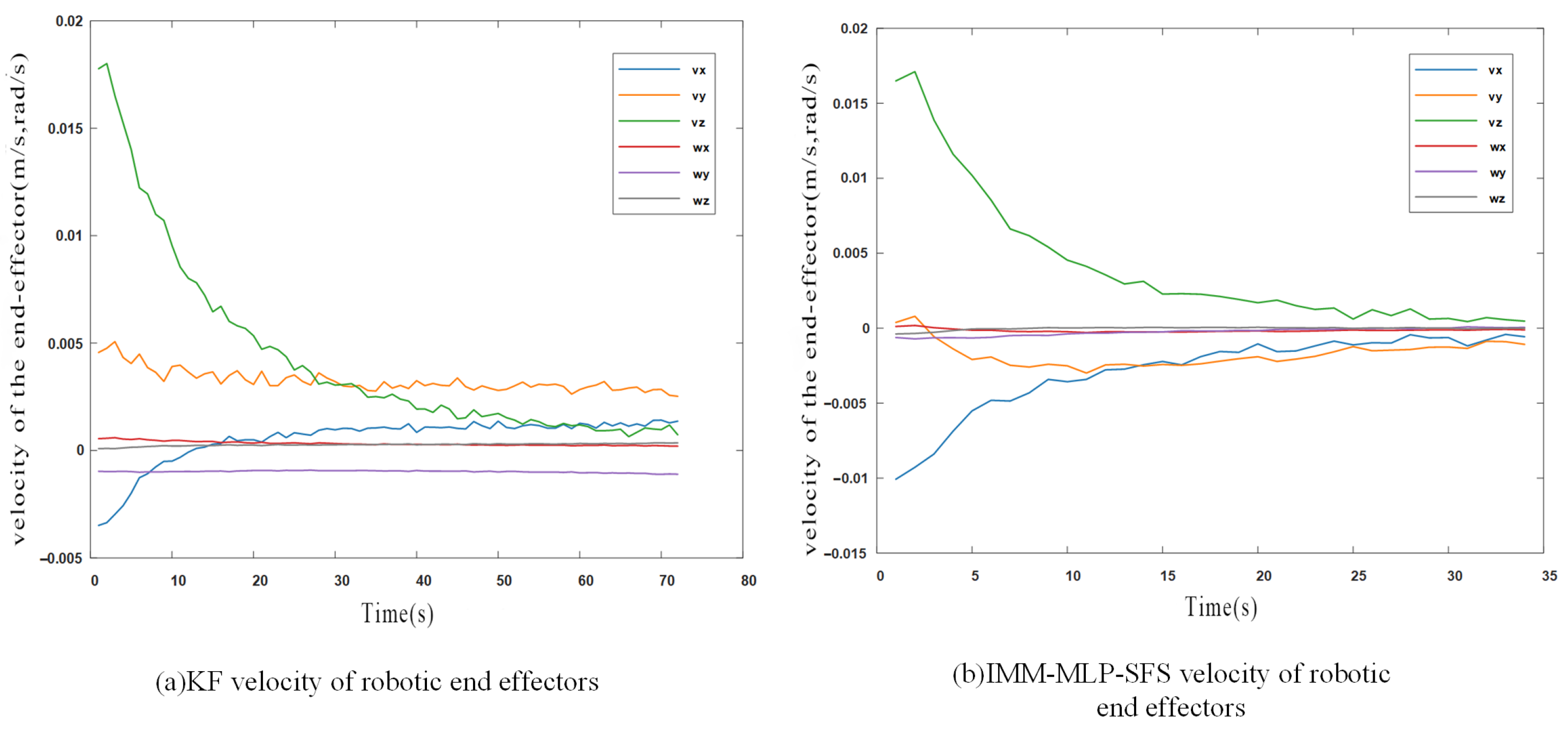
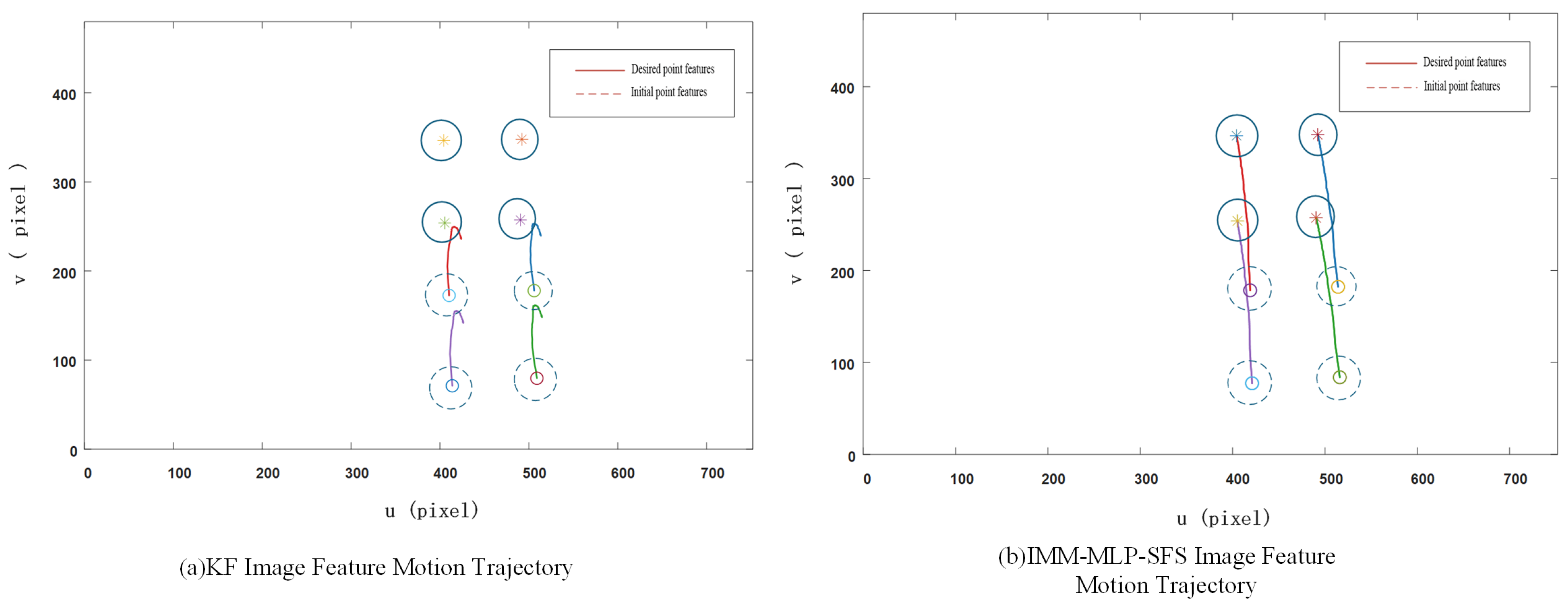
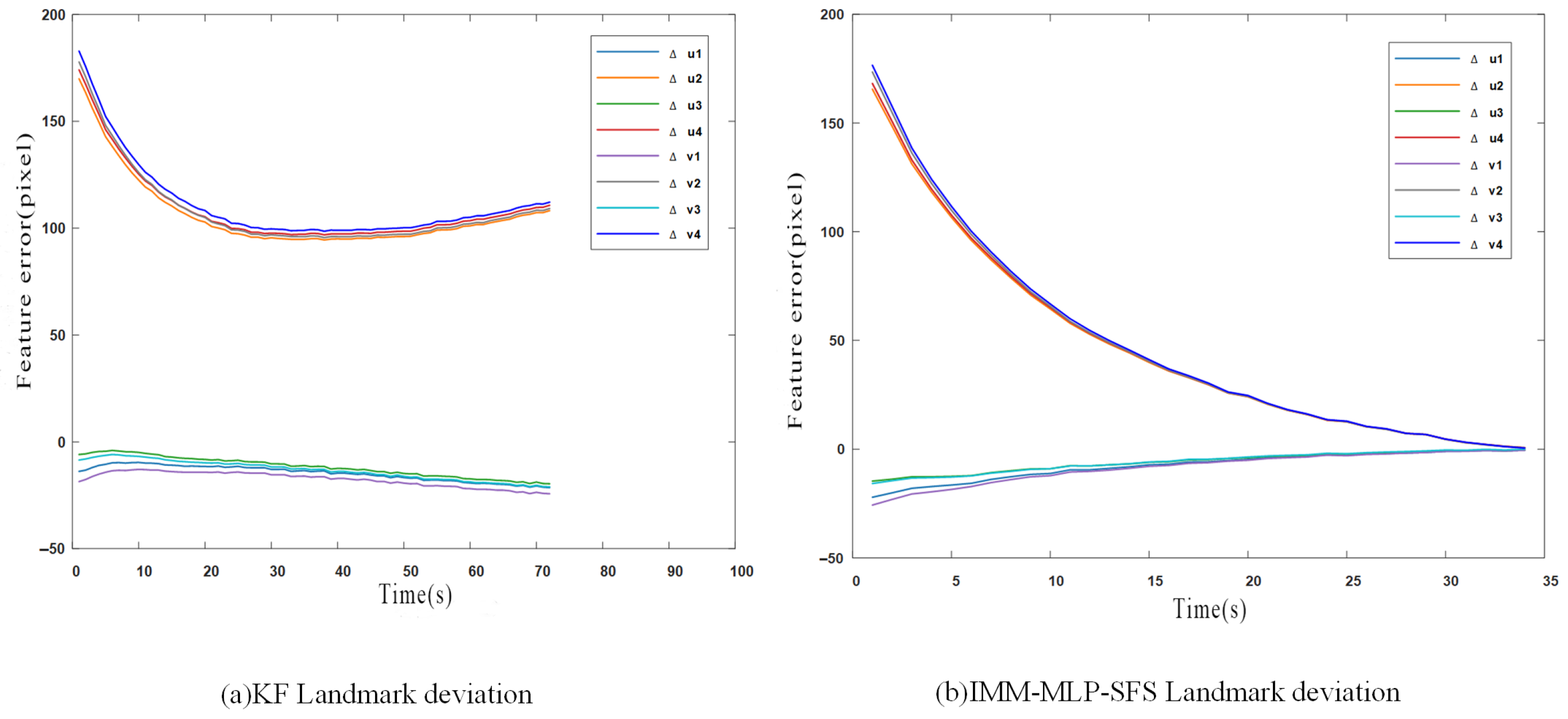
A series of comparative experiments between the conventional KF and the proposed IMM-MLP-SFS algorithm were conducted under non-Gaussian noise conditions, with the results presented in Figure 17, Figure 18 and Figure 19. Figure 17a,b depict the image space trajectories of the KF and IMM-MLP-SFS algorithms, respectively, under identical non-Gaussian noise disturbances. The KF algorithm demonstrates significant susceptibility to noise interference, failing to converge toward the desired feature coordinates. In contrast, the proposed IMM-MLP-SFS method achieves successful target acquisition with a notably smoother and more stable trajectory. Further analysis reveals that under non-Gaussian noise conditions, the KF algorithm’s image error begins to diverge after the eighth iteration, as is visible in Figure 18a. This instability directly impacts the system’s dynamic performance, resulting in the irregular end-effector velocity profile observed in Figure 19a, which fails to reach the desired steady state. Conversely, the proposed algorithm maintains stable operation throughout the task, as evidenced in Figure 18b and Figure 19b, where both feature tracking errors and velocity profiles demonstrate rapid convergence and exceptional robustness against non-Gaussian disturbances. The comparative results clearly indicate that the IMM-MLP-SFS framework substantially outperforms the conventional KF approach in maintaining system stability and precision under challenging non-Gaussian noise environments.

5.4. Composite Motion Experiment

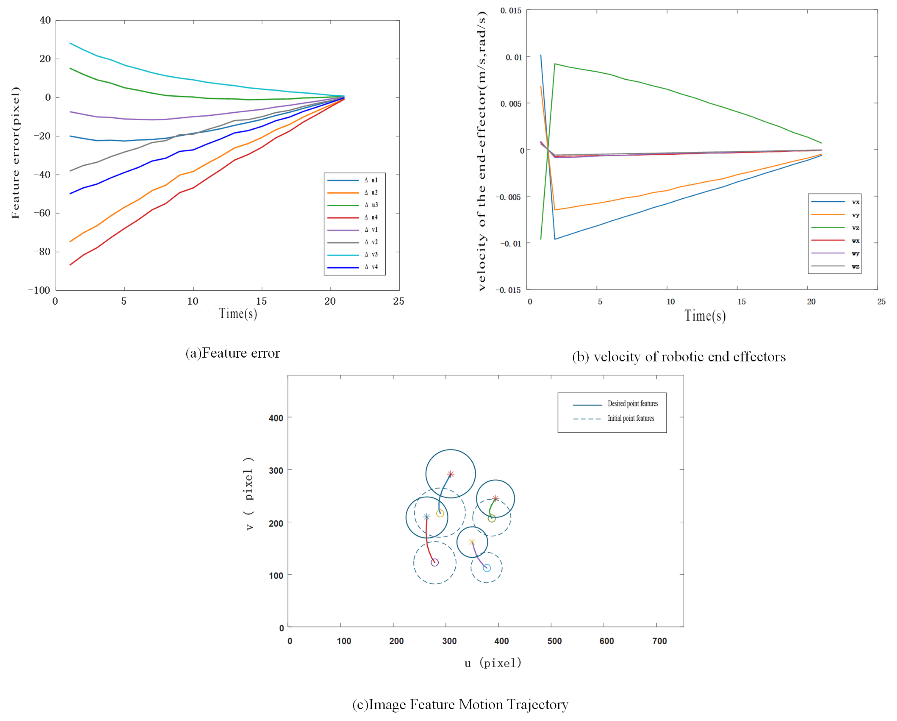
The visual servoing task required transitioning from initial feature points to the desired feature S d 3 = [ 309.3 , 263.6 ; 394.6 , 349.7 ; 291.2 , 209.7 ; 244.9 , 162.1 ] . The results shown in Figure 20 reveal a coordinated composite motion pattern combining translational and rotational components, thereby enabling mutual transformation between the initial and target configurations.
Throughout the entire process, feature deviation remained consistently within 0.8 pixels, while end-effector speed stabilized within ± 0.02 m/s. This high-precision stability validates the IMM-MLP-SFS algorithm’s robust noise suppression capabilities and high-accuracy positioning control, perfectly demonstrating its high-precision visual servoing performance in complex non-Gaussian noise environments.

5.5. Analysis of Computational Complexity and Real-Time Performance

In the robot system, the computational efficiency and real-time performance of the control algorithm are of vital importance. This section conducts a complexity and real-time performance analysis of the proposed IMM-MLP-SFS framework, and combines experimental data to evaluate its feasibility in practical applications.
The computational complexity of the IMM-MLP-SFS framework mainly stems from its three core modules:
(1) Based on the modeling of α -stable distribution and GMM fitting, its complexity is O K · N · d 2 , which corresponds to an offline process.Here, K represents the number of mixture components, N is the number of samples, and d is the feature dimension.
(2) The complexity of the IMM-KF state estimation module is O M · n 3 + m 3 , where the number of models M is small, and n and m are constants, thus having real-time iterative capabilities.
(3) The forward propagation of the MLP compensation module has a linear complexity of O m + n · H + H · n , which is suitable for online execution. Here, the number of input nodes is m + n , and the number of hidden layer nodes is H; meanwhile, SFS optimization, as a global parameter search method, is only used to optimize the weights and biases of the MLP.
To verify the real-time performance of the algorithm framework, we recorded the average execution time of a single iteration of the algorithm on the experimental platform. In the Python environment, by combining the custom API with ROS communication, the total processing time of the IMM-KF and MLP compensation modules was approximately 8–12 ms, which was much lower than the visual sampling period (50 ms), meeting the requirements for real-time control.
Although the SFS optimization process has a high computational cost, its offline execution characteristic enables the online stage to only run the lightweight IMM-KF and MLP forward propagation. This “offline optimization + online inference” design ensures performance while reducing the complexity of the system and improving its real-time performance.

6. Conclusions

This paper has presented an evolutionary neural-enhanced intelligent controller designed to enhance the precision and robustness of robot visual servoing under non-Gaussian noise. The controller integrates α -stable distribution modeling for accurate noise characterization, an IMM-KF for robust state estimation, and an SFS-optimized MLP for adaptive error compensation. Experimental validation confirms that the proposed method outperforms conventional approaches. By adopting the α -stable distribution, it overcomes limitations of traditional Gaussian assumptions and achieves a seamless closed-loop transition from “robust estimation” to “active compensation.” The IMM-MLP-SFS method substantially enhances image Jacobian estimation and end-effector positioning accuracy while tangibly improving system stability under noisy disturbances. These results demonstrate the controller’s effectiveness and its potential for high-precision robotic applications in uncertain industrial environments.
Although the algorithm presented in this paper demonstrates excellent performance in simulations and PC-controlled experiments, its deployment in embedded real-time systems still faces challenges such as computational resources, memory consumption, and sensor synchronization.
Future work will focus on the following aspects: Adopting pruning and quantization techniques to compress MLP and GMM models, achieving lightweight designs to accommodate resource constraints of embedded platforms; implementing multi-sensor time synchronization through hardware triggers and software timestamp alignment to synchronize visual, IMU, and other data, thereby reducing fusion errors; and direct quantitative comparisons with alternative algorithms regarding computational resources (e.g., memory, CPU utilization) will be provided. Concurrently, implementing dynamic occlusion handling will enhance system performance in real-world environments, even when target features are partially or temporarily obscured. These extensions are expected to broaden the applicability of the proposed method within embedded real-time systems.

Author Contributions

Conceptualization, X.R. and H.C.; methodology, X.R.; software, H.Y.; validation, X.R., H.C. and Y.L.; formal analysis, X.R.; investigation, H.C. and Y.L.; resources, X.R.; data curation, H.C. and H.Y.; writing—original draft preparation, H.C.; writing—review and editing, X.R. and H.C.; visualization, H.C. and H.Y.; supervision, X.R.; project administration, X.R.; funding acquisition, X.R. All authors have read and agree to the published manuscript as written consent. All authors have read and agreed to the published version of the manuscript.

Funding

This research was supported by the Department of Science and Technology of Jilin Province. 20230508155RC.

Data Availability Statement

Since there is no suitable data repository for this research area, the data is not publicly available at the time of publication. The data on which the results of this study are based can be obtained by reasonable request to the authors.

Conflicts of Interest

Author Haoyu Yan was employed by the Zhejiang Petrochemical Co., Ltd. The remaining authors declare that the research was conducted in the absence of any commercial or financial relationships that could be construed as a potential conflict of interest.

References

  1. Tao, C.; Li, C.; Xu, H.; Zhu, Z.; Wang, G. A review of digital twin intelligent assembly technology and application for complex mechanical products. Int. J. Adv. Manuf. Technol. 2023, 127, 4013–4033. [Google Scholar] [CrossRef] [Scilit]
  2. Puttero, S.; Verna, E.; Genta, G.; Galetto, M. Collaborative robots for quality control: An overview of recent studies and emerging trends. J. Intell. Manuf. 2025, 1–37. [Google Scholar] [CrossRef] [Scilit]
  3. Parmar, H.; Khan, T.; Tucci, F.; Umer, R.; Carlone, P. Advanced robotics and additive manufacturing of composites: Towards a new era in Industry 4.0. Mater. Manuf. Process. 2022, 37, 483–517. [Google Scholar] [CrossRef] [Scilit]
  4. Banyai, A.D.; Brisan, C. Robotics in physical rehabilitation: Systematic Review. Healthcare 2024, 12, 1720. [Google Scholar] [CrossRef] [Scilit]
  5. Cieslak, C.; Shah, A.; Clark, B.; Childs, P. Wind-Turbine Inspection, Maintenance and Repair Robotic System. In Turbo Expo: Power for Land, Sea, and Air; American Society of Mechanical Engineers: New York, NY, USA, 2023; Volume 87127, p. V014T37A004. [Google Scholar]
  6. Khoei, T.T.; Slimane, H.O.; Kaabouch, N. Deep learning: Systematic review, models, challenges, and research directions. Neural Comput. Appl. 2023, 35, 23103–23124. [Google Scholar] [CrossRef] [Scilit]
  7. Liu, J.; Zhang, T.; Sun, S. Review of deep learning. Geosci. Front. 2024, 15, 101735. [Google Scholar] [CrossRef] [Scilit]
  8. Singh, B.; Kumar, R.; Singh, V.P. Reinforcement learning in robotic applications: A comprehensive survey. Artif. Intell. Rev. 2022, 55, 945–990. [Google Scholar] [CrossRef] [Scilit]
  9. Wu, J.; Jin, Z.; Liu, A.; Yu, L.; Yang, F. A survey of learning-based control of robotic visual servoing systems. J. Franklin Inst. 2022, 359, 556–577. [Google Scholar] [CrossRef] [Scilit]
  10. Nazari, A.A.; Zareinia, K.; Janabi-Sharifi, F. Visual servoing of continuum robots: Methods, challenges, and prospects. Int. J. Med. Robot. Comput. Assist. Surg. 2022, 18, E2384. [Google Scholar] [CrossRef] [Scilit] [PubMed]
  11. Ivan, I.T.; Christian, S. A Theoretical Overview on Kalman Filtering; Vanier College: Montreal, QC, Canada, 2018; Unpublished work. [Google Scholar]
  12. Grewal, M.S. Kalman filtering. In International Encyclopedia of Statistical Science; Springer: Berlin/Heidelberg, Germany, 2025; pp. 1285–1289. [Google Scholar]
  13. Kmich, M.; Karmouni, H.; Harrade, I.; Daoui, A.; Sayyouri, M. Image-Based Visual Servoing Techniques for Robot Control. In Proceedings of the 2022 International Conference on Intelligent Systems and Computer Vision (ISCV), Fez, Morocco, 18–19 May 2022; pp. 1–6. [Google Scholar]
  14. Fourlas, G.K.; Karras, G.C. A survey on fault diagnosis and fault-tolerant control methods for unmanned aerial vehicles. Machines 2021, 9, 197. [Google Scholar] [CrossRef] [Scilit]
  15. Tan, N.; Yu, P.; Zheng, W. Uncalibrated and unmodeled image-based visual servoing of robot manipulators using zeroing neural networks. IEEE Trans. Cybern. 2022, 54, 2446–2459. [Google Scholar] [CrossRef] [Scilit]
  16. Zhou, Y.; Xu, F.; Zhou, Y.; Zhang, Z.; Wang, H. Constrained Image-Based Visual Servoing With a Sampling-Based Planning Framework. IEEE/ASME Trans. Mechatronics 2025, 30, 4899–4909. [Google Scholar] [CrossRef] [Scilit]
  17. Leite, G.R. Uncalibrated Visual Servoing in the Presence of Non-Gaussian Feature Tracking Noise. Doctoral Dissertation, Universidade Federal do Rio Grande do Norte, Natal, Brazil, 2023. [Google Scholar]
  18. Akhtar, S.B.; Ray, R.; Sannyashi, T.S. Adaptive Kalman Filtering for Dynamic Systems with Nonlinearities. J. Innov. Adv. Electron. Front. 2024, 1, 1–8. [Google Scholar] [CrossRef] [Scilit]
  19. Zare, H.; Hajarian, M. An efficient Gauss—Newton algorithm for solving regularized total least squares problems. Numer. Algorithms 2022, 89, 1049–1073. [Google Scholar] [CrossRef] [Scilit]
  20. Liu, Q.; Wang, S.; Wei, Y. A Gauss—Newton method for mixed least squares-total least squares problems. Calcolo 2024, 61, 18. [Google Scholar] [CrossRef] [Scilit]
  21. Tufail, S.; Riggs, H.; Tariq, M.; Sarwat, A.I. Advancements and challenges in machine learning: A comprehensive review of models, libraries, applications, and algorithms. Electronics 2023, 12, 1789. [Google Scholar] [CrossRef] [Scilit]
  22. Long, Z.Z.; Guo, J.L.; Wang, X.M. Noise-Robust Image Jacobian Estimation for Visual Servoing Using BP Neural Network and Robust Kalman Filtering. In Proceedings of the 2025 IEEE International Conference on Industrial Technology (ICIT), Wuhan, China, 26–28 March 2025; pp. 1–5. [Google Scholar]
  23. Przystupa, M.; Dehghan, M.; Jagersand, M.; Mahmood, A.R. Analyzing Neural Jacobian Methods in Applications of Visual Servoing and Kinematic Control. In Proceedings of the 2021 IEEE International Conference on Robotics and Automation (ICRA), Xi’an, China, 30 May–5 June 2021; pp. 14276–14283. [Google Scholar]
  24. Khodarahmi, M.; Maihami, V. A review on Kalman filter models. Arch. Comput. Methods Eng. 2023, 30, 727–747. [Google Scholar] [CrossRef] [Scilit]
  25. Ren, X.; Li, H.; Li, Y. Online Image Jacobian Identification Using Optimal Adaptive Robust Kalman Filter for Uncalibrated Visual Servoing. In Proceedings of the 2017 2nd Asia-Pacific Conference on Intelligent Robot Systems (ACIRS), Wuhan, China, 16–18 June 2017; pp. 53–57. [Google Scholar]
  26. Elfring, J.; Torta, E.; Van De Molengraft, R. Particle filters: A hands-on tutorial. Sensors 2021, 21, 438. [Google Scholar] [CrossRef] [Scilit]
  27. Yu, Z.; Lin, L.; Xue, C.; Zhuo, L.; Yuan, J. Application of Untracked Particle Filter (PSO-UPF) Based on Particle Swarm Optimization in Indoor Target Tracking. In Proceedings of the 2024 20th International Conference on Natural Computation, Fuzzy Systems and Knowledge Discovery (ICNC-FSKD), Guangzhou, China, 27–29 July 2024; pp. 1–6. [Google Scholar]
  28. Leite, G.R.; Araújo, Í.B.Q.; Martins, A.M. Regularized Maximum Correntropy Criterion Kalman Filter for Uncalibrated Visual Servoing in the Presence of Non-Gaussian Feature Tracking Noise. Sensors 2023, 23, 8518. [Google Scholar] [CrossRef] [Scilit] [PubMed]
  29. Zhong, X.; Zhou, Q.; Sun, Y.; Kang, S.; Hu, H. Deep Reinforcement Learning-Based Uncalibrated Visual Servoing Control of Manipulators with FOV Constraints. Appl. Sci. 2025, 15, 4447. [Google Scholar] [CrossRef] [Scilit]
  30. Zhou, Z.; Guo, J.; Zhu, Z.; Guo, H. Uncalibrated visual servoing based on Kalman filter and mixed-kernel online sequential extreme learning machine for robot manipulator. Multimed. Tools Appl. 2024, 83, 18853–18879. [Google Scholar] [CrossRef] [Scilit]
  31. Kang, C.; Qu, X. Visual Servoing Method Based on Partial Convolution Acceleration and Improved Kalman Filter for Robotic Arm. In Proceedings of the 2025 6th International Conference on Electrical Technology and Automatic Control (ICETAC), Nanjing, China, 20–22 June 2025; IEEE: Piscataway, NJ, USA, 2025; pp. 696–703. [Google Scholar]
  32. Dingler, S. State estimation with the Interacting Multiple Model (IMM) method. arXiv 2022, arXiv:2207.04875. [Google Scholar] [CrossRef] [Scilit]
  33. Safar, A.A.; Salih, D.M.; Murshid, A.M. Pattern recognition using the multi-layer perceptron (MLP) for medical disease: A survey. Int. J. Nonlinear Anal. 2023, 14, 1989–1998. [Google Scholar]
  34. El-Shorbagy, M.A.; Bouaouda, A.; Abualigah, L.; Hashim, F.A. Stochastic fractal search: A decade comprehensive review on its theory, variants, and applications. Comput. Model. Eng. Sci. 2025, 142, 2339. [Google Scholar] [CrossRef] [Scilit]
  35. Lu, J. A survey on Bayesian inference for Gaussian mixture model. arXiv 2021, arXiv:2108.11753. [Google Scholar] [CrossRef] [Scilit]
  36. Xie, G.; Sun, L.; Wen, T.; Hei, X.; Qian, F. Adaptive transition probability matrix-based parallel IMM algorithm. IEEE Trans. Syst. Man Cybern. Syst. 2019, 51, 2980–2989. [Google Scholar] [CrossRef] [Scilit]
  37. Leoni, N.; Le Maître, O.; Rodio, M.-G.; Congedo, P.M. Bayesian calibration with adaptive model discrepancy. Int. J. Uncertain. Quantif. 2024, 14, 19–41. [Google Scholar] [CrossRef] [Scilit]
  38. Salimi, H. Stochastic fractal search: A powerful metaheuristic algorithm. Knowl.-Based Syst. 2015, 75, 1–18. [Google Scholar] [CrossRef] [Scilit]
Figure 1. Overall framework of the IMM-MLP-SFS algorithm.
Mathematics 14 00653 g001
Figure 2. α -stable distribution modeling and GMM approximation flowchart.
Mathematics 14 00653 g002
Figure 3. The IMM-MLP-SFS algorithm block diagram.
Mathematics 14 00653 g003
Figure 4. Scenario 1: Simulation Results Based on the KF Algorithm.
Mathematics 14 00653 g004
Figure 5. Scenario 1: simulation results based on the IMM algorithm.
Mathematics 14 00653 g005
Figure 6. Scenario 1: Simulation results based on the IMM-MLP-SFS algorithm.
Mathematics 14 00653 g006
Figure 7. Scenario 2: Trajectories of image features under non-Gaussian noise for four algorithms.
Mathematics 14 00653 g007
Figure 8. Scenario 2: Image feature error curves under non-Gaussian noise for four algorithms.
Mathematics 14 00653 g008
Figure 9. Scenario 2: Speed curves of the robot end-effector under non-Gaussian noise for four algorithms.
Mathematics 14 00653 g009
Figure 10. Scenario 2: Trajectories in Cartesian space under non-Gaussian noise for four algorithms.
Mathematics 14 00653 g010
Figure 11. Scenario 3: Robustness limit performance testing of different algorithms.
Mathematics 14 00653 g011
Figure 12. Scenario 3: Generalization capability of the IMM-SFS-MLP algorithm.
Mathematics 14 00653 g012
Figure 13. Visual servo experiment setup.
Mathematics 14 00653 g013
Figure 14. Comparison of image feature motion trajectories between IMM and IMM-MLP-SFS under non-Gaussian noise conditions.
Mathematics 14 00653 g014
Figure 15. Comparison of image feature errors between IMM and IMM-MLP-SFS under non-Gaussian noise conditions.
Mathematics 14 00653 g015
Figure 16. Comparison of robot end-effector velocity between IMM and IMM-MLP-SFS under non-Gaussian noise.
Mathematics 14 00653 g016
Figure 17. Comparison of image feature trajectories between KF and IMM-MLP-SFS under non-Gaussian noise.
Mathematics 14 00653 g017
Figure 18. Comparison of image feature errors between KF and IMM-MLP-SFS under non-Gaussian noise conditions.
Mathematics 14 00653 g018
Figure 19. Comparison of robot end-effector velocity between KF and IMM-MLP-SFS under non-Gaussian noise.
Mathematics 14 00653 g019
Figure 20. Performance of the IMM-MLP-SFS algorithm under rotational positioning.
Mathematics 14 00653 g020
Table 1. Comparison of different methods.
Iterations (s)Convergence (s)Magnitude of Fluctuation (m/s)
KF150200[−0.223, 0.191]
IMM160165[−0.034, 0.042]
SVSF-KF200200[−0.051, 0.022]
MCKF320175[−0.013, 0.015]
ARKF315235[−0.149, 0.147]
IMM-MLP-SFS (our)200150[−0.013, 0.023]
Disclaimer/Publisher’s Note: The statements, opinions and data contained in all publications are solely those of the individual author(s) and contributor(s) and not of MDPI and/or the editor(s). MDPI and/or the editor(s) disclaim responsibility for any injury to people or property resulting from any ideas, methods, instructions or products referred to in the content.