Fuzzy Improved Distributions for Exceedance Counts in Order Statistic Intervals

Abstract

We study exceedance counts for order statistic intervals when boundary uncertainty is modeled through a fuzzy improved distribution function. In an ordinary setting, whether an observation falls below a threshold is decided by a crisp comparison, which can be unstable when specifications are vague, subject to tolerance bands, or expressed linguistically. We replace the crisp rule by a graded membership function and use the fuzzy improved cumulative distribution function $F_{\mu }$. From an initial independent and identically distributed sample, with ordinary cumulative distribution function F, we form the random interval between the r-th and s-th order statistics, and we count how many of m independent newcomers fall inside this interval. Newcomers follow either the ordinary model ($Q=F$) or the fuzzy improved model ($Q=F_{\mu }$). We derive exact finite-sample formulas, moments, and a distribution-free representation based on a probability integral transform, which yields the large-m limit law of the newcomer proportion. Numerical illustrations for exponential and uniform distributions show how fuzzification reshapes the distribution and can materially change predictive dispersion of exceedance counts.

1. Introduction

Exceedance statistics based on order statistic intervals are widely used in reliability and quality-control settings, for example, when tolerance or invariant intervals are constructed from an initial sample and the number of newcomers falling into the interval is evaluated [1,2,3]. Such methods rely on the distribution theory of order statistics from an independent and identically distributed (iid) sample and remain fundamental for analyzing component lifetimes and coherent systems, including k-out-of-n:G systems [4,5].

A persistent limitation of ordinary exceedance formulations is that they are built on crisp comparisons, such as $I\{X\le t\}$, and therefore assume sharply defined thresholds and precisely specified distribution functions. In many engineering and medical contexts, threshold comparisons are inherently vague due to linguistic specifications (e.g., “slightly early”), sensor tolerances, and gradual operational drift. This boundary uncertainty means that minor variations near the threshold can trigger a binary switch (0 to 1), producing overconfident exceedance predictions and a significant underestimation of dispersion. Fuzzy set theory provides a principled way to model graded membership and partial truth values [6,7,8], and fuzzy-based tools are already used in reliability contexts such as fuzzy fault trees and fuzzy Markov models [9,10,11,12]. These settings motivate exceedance models that remain probabilistic but explicitly account for threshold vagueness, so that exceedance predictions reflect realistic uncertainty rather than an artifact of crisp indicator comparisons.

In this paper, “fuzziness” is not introduced by replacing probabilistic uncertainty with subjective degrees of belief; rather, it enters through the comparison rule used to decide whether an observation falls below a threshold [6,7,8]. Concretely, the event $\{X\le t\}$ is replaced by a graded event whose membership depends on $X{\le }_{\mu }t$ [13]. This modeling choice separates two sources of uncertainty, namely sampling variability of the order statistic order statistic interval and boundary uncertainty in the thresholding mechanism itself [2,3]. The resulting model remains fully probabilistic; the fuzzy improved function $F_{\mu }$ is an ordinary cdf, and exceedance counts are random variables with well-defined finite-sample and asymptotic distributions [3,14].

To incorporate graded comparisons at the distribution level while preserving probabilistic tractability, this paper adopts the fuzzy improved distribution function introduced in [13]. A crisp relation $X\le t$ is replaced by a graded relation $X{\le }_{\mu }t$ determined by a membership function $\mu (x,t)=g(t-x)I\{t\ge x\}$, where g is nondecreasing. The fuzzy improved cumulative distribution function (cdf) is $F_{\mu }\left(t\right)=P\left\{X{\le }_{\mu }t\right\}$, which encodes the strength of the comparison through g while remaining a valid cdf.

The role of g admits a useful statistical interpretation that also guides its specification. Since $\mu (x,t)=g(t-x)I\{t\ge x\}$ depends on $t-x$, one may view g as a soft indicator kernel that replaces the crisp step function [6]. Equivalently, g can be regarded as encoding a non-negative “tolerance” (or slack) $∆$ that softens the boundary in the comparison $X\le t$: instead of a binary switch at a single point, the decision transitions gradually over a range whose width is governed by the scale of $∆$. The crisp model is recovered as this tolerance shrinks toward 0, making the transition in g arbitrarily steep. This connects the graded relation $X{\le }_{\mu }t$ to a concrete boundary-uncertainty mechanism while keeping all objects within ordinary probability theory [13].

This interpretation also suggests practical calibration rules. In engineering settings, domain specifications often provide a tolerance scale (e.g., a band of width $\delta$ around the nominal threshold) or target transition probabilities; these can be translated into constraints such as requiring $g\left(\delta \right)=p$ for a chosen $p\in (0,1)$ [15,16]. When repeated measurements or paired judgments are available, the parameters of a parametric family $g(u;\theta )$ can be estimated from data by likelihood methods through the induced density $f_{\mu }$. When calibration information is limited, $\theta$ can be treated as a sensitivity parameter and varied to assess robustness of exceedance predictions; importantly, the distributional results developed in this paper hold for any nondecreasing g satisfying the boundary conditions of [13], so the theory does not depend on a single functional choice.

The main question is: How do observations from a fuzzy improved distribution behave relative to order statistic intervals formed from an ordinary sample? Let $X_1,\dots ,X_n$ be iid random variables with cdf F, and let $X_{1:n}\le \cdots \le X_{n:n}$ denote the order statistics. Fix $1\le r<s\le n$ and consider the random interval $(X_{r:n},X_{s:n})$. Independently, observe m newcomers with cdf Q. In the ordinary cdf, $Q=F$ and the exceedance count in the interval is denoted by $S_m$. In the fuzzy improved model, $Q=F_{\mu }$ and the corresponding count is denoted by $S_m^{\mu }$. Conditionally on $(X_{r:n},X_{s:n})$, both $S_m$ and $S_m^{\mu }$ are binomial. Unconditionally, they follow mixed binomial laws because the inclusion probability is random through the random endpoints; in the ordinary case $Q=F$, this reduces to the beta-binomial distribution.

Ordinary exceedance-count theory for invariant order statistic intervals is well developed when newcomers follow an ordinary (crisp) probabilistic model, with particularly sharp distribution-free results in the ordinary case $Q=F$ [3,17]. In these models, the only randomness is sampling variability of the order statistic intervals and the newcomers sample; the comparison rule itself is not uncertain. Separately, fuzzy improved distributions and fuzzy order statistic formulations have been introduced to encode graded comparisons through a membership function and to study how fuzzification alters distributional shape, tail behavior, and endpoint effects [13]. What has been missing is an exceedance-count theory in which the order statistic interval remains ordinary, while the newcomers are modeled through the fuzzy improved cdf $F_{\mu }$. This setting is natural in practice when existing data are well modeled by an ordinary distribution, yet the operational meaning of “exceeding” a threshold is vague. The paper fills this gap by developing finite-sample and asymptotic laws of the exceedance count under fuzzy improved observations and by quantifying how fuzzification changes predictive dispersion relative to the ordinary distribution.

The main contributions of this paper are as follows. First, we formulate exceedance counts for the ordinary order statistic interval $(X_{r:n},X_{s:n})$ when newcomers follow either the ordinary case $Q=F$ or the fuzzy improved model $Q=F_{\mu }$ induced by a membership function $\mu$. Second, we derive exact finite-sample representations for the exceedance counts, preserving the conditional binomial structure while showing that the unconditional laws are mixed binomials. Third, we obtain a distribution-free representation via the probability integral transform $(W,Z)=(F\left(X_{r:n}\right),F\left(X_{s:n}\right))$, leading to a large-m limit distribution for the exceedance proportion. Fourth, worked exponential and uniform examples are provided, demonstrating that fuzzification can introduce bounded support and can yield more conservative predictive dispersion for exceedance counts.

This paper is organized as follows. Section 2 reviews background on exceedance statistics based on invariant order statistic intervals, introduces the fuzzy improved distribution function $F_{\mu }$, and summarizes three formulations of fuzzy order statistics used for interpretation. Section 3 derives the finite-sample representation and pmf of the fuzzy newcomer exceedance count $S_m^{\mu }$ for the ordinary interval $(X_{r:n},X_{s:n})$ and presents worked numerical examples under exponential and uniform distributions. Section 4 studies the large-m behavior of the newcomer proportion ${\zeta }_m^{\mu }=S_m^{\mu }/m$ using a distribution-free probability integral transform, and provides limit distributions and moment expressions together with numerical illustrations. Section 5 synthesizes the numerical findings and compares how the choice of membership function g reshapes the predictive distribution relative to the ordinary cdf. Section 6 gives illustrative applications (reliability planning and spam filtering) that clarify modeling choices and interpretation. Section 7 concludes.

2. Methodology

This section summarizes exceedance counts under ordinary newcomer models, the construction and properties of the fuzzy improved cdf $F_{\mu }$, and notions of fuzzy order statistics used later for interpretation and applications.

2.1. Exceedance Statistics

Order statistics are fundamental in reliability analysis because many system lifetimes can be written in terms of component lifetimes; for example, the lifetime of an $(n-k+1)$-out-of-n system is the kth order statistic of the component lifetimes [16,18]. Order statistic intervals are also central in tolerance and invariant-interval theory, where one studies the number of newcomers falling into an interval constructed from an iid sample [14].

Let $X_1,X_2,\dots ,X_n$ be an iid sample from the distribution function $F,$ that belongs to a class of distribution $\mathcal{F}$. Let $f_1$ and $f_2$ be two n-variate real functions satisfying

$$f_1(u_1,u_2,\dots ,u_n)\le f_2(u_1,u_2,\dots ,u_n),\forall (u_1,u_2,...,u_n)\in {\mathbb{R}}^n.$$

If

$$P\{X_{n+1}\in (f_1(X_1,X_2,\dots ,X_n),f_2(X_1,X_2,\dots ,X_n))\}=\alpha ,\forall F\in \mathcal{F}.$$

then $(f_1(X_1,X_2,\dots ,X_n),f_2(X_1,X_2,\dots ,X_n))$ is an invariant confidence interval containing the ordinary probability mass of the random variable X having distribution function F. It is proved in [19] that if $f_1$ and $f_2$ are two continuous and symmetric functions of n variables, then the only invariant confidence interval for a class of all continuous cdfs $\mathcal{F}={\mathcal{F}}_c,$ is the interval $(X_{r:n},X_{s:n}),$ where $X_{r:n}$ and $X_{s:n}$ are the rth and sth order statistics of the sample $X_1,X_2,\dots ,X_n$ and

$$P\{X_{r:n}<X_{n+1}<X_{s:n}\}={\displaystyle \frac{s-r}{n+1}}.$$

(1)

This ordinary setup is visualized in Figure 1. In survival analysis, quality control, and reliability, it is often important to quantify how many observations from a new sample fall into an interval constructed from an initial sample.

To write unconditional exceedance probabilities compactly, we use the functional $H_F\left(·\right)$. Considering the distribution function F for any integrable n-variate function $\phi (u_1,\dots ,u_n)$,

$$H_F\left(\phi \right)=\int \cdots \int \phi (u_1,\dots ,u_n)dF\left(u_1\right)\cdots dF\left(u_n\right),$$

so that $H_F$ is linear ($H_F(c_1{\phi }_1+c_2{\phi }_2)=c_1{H}_F\left({\phi }_1\right)+c_2{H}_F\left({\phi }_2\right)$) and normalized ($H_F\left(1\right)=1$).

Let $X_1,\dots ,X_n$ be iid random variables with cdf $F,$ and $X_{n+1},\dots ,X_{n+m}$ be iid random variables with cdf $Q.$ Assume that $X_1,\dots ,X_n$ and $X_{n+1},\dots ,X_{n+m}$ are independent. Let $f_1,f_2:{\mathbb{R}}^n\to \mathbb{R}$ be measurable functions satisfying

$$f_1(u_1,\dots ,u_n)\le f_2(u_1,\dots ,u_n)\forall (u_1,\dots ,u_n)\in {\mathbb{R}}^n.$$

For $k=1,\dots ,m$, define the events

$$A_k=\left\{f_1(X_1,\dots ,X_n)<X_{n+k}<f_2(X_1,\dots ,X_n)\right\}.$$

Then, with $\overline{u}=(u_1,\dots ,u_n)$,

$$p=P\left(A_k\right)=H_F\left\{Q\left(f_2\left(\overline{u}\right)\right)-Q\left(f_1\left(\overline{u}\right)\right)\right\}=:H_F\left\{Q_{f_1}^{f_2}\right\},$$

which does not depend on k. Consider,

$${\xi }_k=\left\{\begin{array}{cc}1\hfill & \mathrm{if}{A}_k\mathrm{occurs}\hfill \\ 0\hfill & \mathrm{otherwise}\hfill \end{array}\right.,k=1,2,\dots ,m.$$

and define

$$S_m=\sum _{k=1}^m{\xi }_k\in \{0,1,\dots ,m\}.$$

The finite distribution of $S_m$ is

$$\begin{array}{ccc}\hfill P\{S_m& =& k\}=\left({\displaystyle \genfrac{}{}{0pt}{}{m}{k}}\right)H_F\left\{{\left[Q_{f_1}^{f_2}\left(\overline{u}\right)\right]}^k{[1-Q_{f_1}^{f_2}\left(\overline{u}\right)]}^{m-k}\right\},k=0,1,\dots ,m.\hfill \end{array}$$

where $Q_{f_1}^{f_2}\left(\overline{u}\right):=Q\left(f_2\left(\overline{u}\right)\right)-Q\left(f_1\left(\overline{u}\right)\right)$ and $\overline{u}=(u_1,\dots ,u_n)$. Note that ${\xi }_1,{\xi }_2,\dots ,{\xi }_m$ are dependent random variables and so $S_m$ is not binomial [14]. For an asymptotic distribution let ${\zeta }_m=S_m/m$ and define, for $0\le x\le 1$,

$$C\left(x\right)=P\left\{Q_{f_1}^{f_2}(X_1,\dots ,X_n)\le x\right\}.$$

Then,

$$\underset{m\to \infty }{lim}\underset{0\le x\le 1}{sup}\left|P\{{\zeta }_m\le x\}-C\left(x\right)\right|=0.$$

If $f_1(X_1,X_2,\dots ,X_n)=X_{i:n}$ and $f_2(X_1,X_2,\dots ,X_n)=X_{j:n},$ $1\le i<j\le n,$ and if $F=Q,$ then

$$Q\left(X_{j:n}\right)-Q\left(X_{i:n}\right)\mathrm{has}\mathrm{a}\mathrm{Beta}(j-i,n-j+i+1)\mathrm{distribution}.$$

Let $f_1\left(\overline{X}\right)=X_{r:n}$ and $f_2\left(\overline{X}\right)=X_{s:n}$ with $1\le r<s\le n$, and $X_{n+1},\dots ,X_{n+m}$ iid newcomers with cdf F. Then

$$p:=F\left(X_{s:n}\right)-F\left(X_{r:n}\right)\mathrm{has}\mathrm{a}\mathrm{Beta}(\alpha ,\beta )\mathrm{distribution},\alpha =s-r,\beta =n-s+r+1,$$

and therefore the unconditional distribution of $S_m$ is beta-binomial:

$$P\{S_m=k\}=\left({\displaystyle \genfrac{}{}{0pt}{}{m}{k}}\right){\displaystyle \frac{B(k+\alpha ,m-k+\beta )}{B(\alpha ,\beta )}},k=0,1,\dots ,m.$$

Conditionally on $(X_1,\dots ,X_n)$, the endpoints $f_1\left(\overline{X}\right),f_2\left(\overline{X}\right)$ are fixed, and since the newcomers $X_{n+1},\dots ,X_{n+m}$ have cdf Q and independent of $(X_1,\dots ,X_n)$, the events $A_k=\{f_1\left(\overline{X}\right)<X_{n+k}<f_2\left(\overline{X}\right)\}$ are independent with $P(A_k\mid X_1,\dots ,X_n)=Q\left(f_2\left(\overline{X}\right)\right)-Q\left(f_1\left(\overline{X}\right)\right)=:p\left(\overline{X}\right)$. Conditionally on $(X_1,\dots ,X_n)$, $S_m$ is binomial with parameters m and $p\left(\overline{X}\right)$. Unconditionally, $S_m$ has a mixed-binomial distribution. Moreover, ${\zeta }_m=S_m/m$ converges in distribution to $p\left(\overline{X}\right)$, with limit cdf $C\left(x\right)=P\{p\left(\overline{X}\right)\le x\}$. In the ordinary case $Q=F$ with $f_1\left(\overline{X}\right)=X_{r:n}$ and $f_2\left(\overline{X}\right)=X_{s:n}$, p has a $\mathrm{Beta}(s-r,n-s+r+1)$ distribution and thus

$$C\left(x\right)=I_x\left(s-r,n-s+r+1\right),$$

where $B_y(a,b)={\int }_0^y{t}^{a-1}{(1-t)}^{b-1}dt$ is the (unregularized) incomplete beta, $B(a,b)$ is the beta function, and $I_x(a,b)=B_x(a,b)/B(a,b)$ is the regularized form.

2.2. Fuzzy Improved Distribution

Following Bayramoglu [13], let X be a random variable with cdf F. Let

$$a=inf\{x:F(x)>0\},b=sup\{x:F(x)<1\},$$

allowing $a=-\infty$ and/or $b=+\infty$, and denote the support set by $A=[a,b]$. Consider a fuzzy partial ordering on A with membership function

$$\mu (x,t)=\left\{\begin{array}{cc}g(t-x),\hfill & t\ge x,\hfill \\ 0,\hfill & t<x,\hfill \end{array}\right.$$

(2)

where g is nondecreasing and continuous. If $b<\infty$, g is defined on $[0,b-a]$ and satisfies $g\left(0\right)=0$ and $g(b-a)=1$. If $b=\infty$, g is defined on $[0,\infty )$ with $g\left(0\right)=0$ and ${lim}_{u\to \infty }g\left(u\right)=1$.

The fuzzy improved cdf is defined by

$$F_{\mu }\left(t\right)=P\left\{X{\le }_{\mu }t\right\}=\left\{\begin{array}{cc}0,\hfill & t\le a,\hfill \\ {\displaystyle {\int }_a^{t}g(t-x)dF\left(x\right),}\hfill & a<t<b,\hfill \\ 1,\hfill & t\ge b,\hfill \end{array}\right.$$

(3)

On bounded supports ($b<\infty$), $F_{\mu }$ is nondecreasing and right-continuous and may have a jump at $t=b$. In particular, the left limit

$$F_{\mu }\left(b^{-}\right):=\underset{t\to b}{lim}{\int }_a^{t}g(t-x)dF\left(x\right)$$

can be strictly less than 1, while $F_{\mu }\left(b\right)=1$ by the definition for $t\ge b$. Assume F is absolutely continuous with probability density function (pdf) f and g is differentiable. Then, for $t\in (a,b)$,

$$\begin{array}{cc}\hfill f_{\mu }\left(t\right)& ={\displaystyle \frac{d}{dt}}{\int }_a^{t}g(t-x)dF\left(x\right)\hfill \\ \hfill & ={\int }_a^t{\displaystyle \frac{d}{dt}}g(t-x)dF\left(x\right)+g\left(0\right)f\left(t\right)\hfill \\ \hfill & ={\int }_a^t{g}^{\prime }(t-x)dF\left(x\right)\hfill \end{array}$$

(4)

since $g\left(0\right)=0$. In the absolutely continuous case this becomes

$$f_{\mu }\left(t\right)={\int }_a^t{g}^{\prime }(t-x)f\left(x\right)dx,t\in (a,b),$$

(5)

and $f_{\mu }\left(t\right)=0$ for $t\notin (a,b)$.

2.3. Choosing and Estimating the Membership Function

To use the exceedance-count model in applications, one must specify the graded-comparison mechanism through a membership function Equation (2) [13]. We recommend choosing g by linking it to an interpretable tolerance (or slack) variable [6]. Specifically, if $∆\ge 0$ is independent of X and $\mu (x,t)$ is the cdf of $∆$,

$$g\left(u\right)=P(∆\le u),u\ge 0,$$

then the fuzzy improved cdf satisfies

$$F_{\mu }\left(t\right)={\int }_a^{t}g(t-x)dF\left(x\right)=P(X+∆\le t),$$

so g encodes the scale and shape of boundary uncertainty in the comparison rule. This interpretation provides a principled way to specify a parametric family $g(u;\theta )$: the parameter $\theta$ controls the spread of $∆$ (hence the “fuzziness width”) and can be calibrated from engineering tolerances or pilot data. For example, if domain knowledge suggests that exceedance decisions should be “mostly crisp” beyond a tolerance $\delta >0$, one may impose quantile constraints such as $g(\delta ;\theta )=p$ for a chosen $p\in (0,1)$ [20]. For inference from data, we model the newcomer distribution as

$$Q\left(t\right)=F_{\mu }(t;\theta ,\psi ),F_{\mu }(t;\theta ,\psi )={\int }_a^{t}g(t-x;\theta )dF(x;\psi ),$$

where $F(t;\psi )$ is a baseline family when F is not assumed known. Under absolute continuity and differentiability

$$f_{\mu }(t;\theta ,\psi )={\int }_a^t{\displaystyle \frac{\partial }{\partial t}}g(t-x;\theta )f(x;\psi )dx,$$

and $(\theta ,\psi )$ can be estimated by maximum likelihood from observations $X_1,\dots ,X_N$:

$$(\widehat{\theta },\widehat{\psi })=arg\underset{\theta ,\psi }{max}\sum _{i=1}^{N}ln{f}_{\mu }(X_i;\theta ,\psi ).$$

(Section 6.1 uses the corresponding right-censored likelihood.)

In practice g is a modeling choice, so it is important to assess robustness of exceedance predictions to plausible alternatives. A simple workflow is: (i) fit one or more candidate families $g(u;\theta )$ (e.g., exponential-type, polynomial-type on bounded supports), (ii) recompute key predictive summaries of $S_m^{\mu }$ or ${\zeta }_m^{\mu }$ (means, variances, and tail probabilities), and (iii) report the resulting range as a sensitivity band. Because all distributional results in Section 3 and Section 4 depend on fuzzification only through Equation (13) and, hence, through Equation (14), this robustness check can be implemented by varying $\theta$ (and/or the family of g) and re-evaluating the induced $\phi$.

For example with $g(u;\theta )=1-e^{-\theta u}$ for $u\ge 0$, $\theta >0$, we have $g^{\prime }(u;\theta )=\theta e^{-\theta u}$ and, hence

$$f_{\mu }(t;\theta ,\psi )={\int }_a^t\theta e^{-\theta (t-x)}f(x;\psi )dx.$$

If, additionally, $F(x;\psi )=1-e^{-x}$ (exponential baseline), then for $\theta \ne 1$

$$F_{\mu }(x;\theta )=1-e^{-x}-{\displaystyle \frac{1}{\theta -1}}(e^{-x}-e^{-\theta x}),f_{\mu }(x;\theta )={\displaystyle \frac{\theta }{\theta -1}}(e^{-x}-e^{-\theta x}),$$

with the case $\theta =1$ obtained by continuity.

2.4. Fuzzy Order Statistics

Bayramoglu [13] introduced ways to define order statistics under a fuzzy ordering. Type 1 studies order statistics of the fuzzy improved variable $X_{\mu }$; Type 2 fuzzifies the cdf of the ordinary order statistics of X; Type 3 applies fuzzy pairwise comparisons directly to the original sample $\left\{X_i\right\}$, yielding fuzzy ranks.

2.4.1. Type 1: Order Statistics of $X_{\mu }$

Let $Y_1,\dots ,Y_n$ be iid copies of $X_{\mu }$ with cdf $F_{\mu }$ and probability density function (pdf) $f_{\mu }$. For $1\le r\le n$

$$F_{Y_{r:n}}\left(x\right)=n\left({\displaystyle \genfrac{}{}{0pt}{}{n-1}{r-1}}\right){\int }_a^x{\left[F_{\mu }\left(u\right)\right]}^{r-1}{[1-F_{\mu }\left(u\right)]}^{n-r}{f}_{\mu }\left(u\right)du$$

(6)

$$f_{Y_{r:n}}\left(x\right)=n\left({\displaystyle \genfrac{}{}{0pt}{}{n-1}{r-1}}\right){\left[F_{\mu }\left(x\right)\right]}^{r-1}{[1-F_{\mu }\left(x\right)]}^{n-r}{f}_{\mu }\left(x\right).$$

(7)

2.4.2. Type 2: Fuzzy CDF of Order Statistics

Let $X_1,\dots ,X_n$ be iid random variables from cdf F on $[a,b]$, with ordinary order statistics $X_{1:n}\le \cdots \le X_{n:n}$. With fuzzy ordering membership function $\mu (x,t)$

$$F_{[n:n]}\left(x\right)=P\left\{X_{n:n}{\le }_{\mu }x\right\}=n{\int }_a^{x}g(x-u){\left[F\left(u\right)\right]}^{n-1}dF\left(u\right),$$

$$F_{[1:n]}\left(x\right)=P\left\{X_{1:n}{\le }_{\mu }x\right\}=n{\int }_a^{x}g(x-u){[1-F\left(u\right)]}^{n-1}dF\left(u\right),$$

and, for $1\le r\le n$

$$F_{[r:n]}\left(x\right)=n\left({\displaystyle \genfrac{}{}{0pt}{}{n-1}{r-1}}\right){\int }_a^{x}g(x-u){\left[F\left(u\right)\right]}^{r-1}{[1-F\left(u\right)]}^{n-r}dF\left(u\right).$$

(8)

2.4.3. Type 3: Fuzzy Pairwise Ranking and Fuzzy Ranks

For $x,y\in [a,b]$, define the pairwise comparison grade $\mu (x,y)=g(y-x)I\{y\ge x\}$. Following [13], fuzzy ranks are obtained by aggregating these pairwise grades across the sample, and $X^{\left(r\right)}$ denotes the r-th fuzzily smallest observation.

$$P\{X^{\left(1\right)}\le x\}=1-n{\int }_x^b{\left({\int }_t^{b}g(y-t)dF\left(y\right)\right)}^{n-1}dF\left(t\right),$$

and, for $1\le r\le n$,

$$\begin{array}{c}\hfill P\{X^{\left(r\right)}\le x\}=n\left({\displaystyle \genfrac{}{}{0pt}{}{n-1}{r-1}}\right){\int }_a^x{\left({\int }_a^{t}g(t-y)dF\left(y\right)\right)}^{r-1}{\left({\int }_t^{b}g(y-t)dF\left(y\right)\right)}^{n-r}dF\left(t\right).\end{array}$$

(9)

Remark 1.

In this paper we do not use fuzzy order statistic Types 1–3 to construct the order statistic interval. Instead, we keep the order statistic interval $(X_{r:n},X_{s:n})$ as an ordinary invariant order-statistic interval obtained from the baseline sample with cdf F [2,19], and we introduce fuzziness only through the newcomer model via the fuzzy improved cdf $F_{\mu }$. This choice is motivated by applications in which reference limits are fixed by established procedures on crisp data, while uncertainty enters primarily through the operational meaning of threshold comparisons for new items (tolerance bands, linguistic specifications, or gradual drift) [11,16,21]. From a methodological standpoint, retaining an ordinary order statistic interval preserves the classical distribution-free structure under the probability integral transform $(W,Z)=(F\left(X_{r:n}\right),F\left(X_{s:n}\right))$ [1], while the effect of fuzzification appears only through the induced mapping $\phi \left(w\right)=F_{\mu }\left(F^{-1}\left(w\right)\right)$. If the interval endpoints were fuzzified as well (e.g., by using Type 1 or Type 2 order statistics as endpoints, or by fuzzy ranks in Type 3) [13], then both the order statistic interval and the newcomer mechanism would depend on μ, and changes in the exceedance count would mix two distinct sources of fuzzification. The present configuration, therefore, provides a clean framework for quantifying how fuzzy improved modeling of newcomers reshapes exceedance-count predictions relative to the ordinary benchmark [3,14].

3. Distribution of Fuzzy Newcomers in an Ordinary Order Statistic Interval

The central problem addressed in this paper is the distribution of the newcomer count in the random interval $(X_{r:n},X_{s:n})$ when newcomers follow the fuzzy improved cdf $F_{\mu }$. Let $X_1,\dots ,X_n$ be an iid sample from the cdf F with pdf f. Let $X_{r:n}$ and $X_{s:n}$ be the rth and sth order statistics from this sample, where $1\le r<s\le n$. Let $X_{n+1},\dots ,X_{n+m}$ be a second sample of m iid newcomers, drawn independently from the fuzzy improved cdf $F_{\mu }$. Define

$$S_m^{\mu }=\sum _{i=1}^m{\xi }_i^{\mu },{\xi }_i^{\mu }:=I\{X_{r:n}<X_{n+i}<X_{s:n}\},i=1,\dots ,m.$$

In the ordinary case, let $Y_1,\dots ,Y_m$ be iid random variables with cdf F, independent of $(X_1,\dots ,X_n)$, and define

$${\xi }_i:=I\{X_{r:n}<Y_i<X_{s:n}\},S_m:=\sum _{i=1}^m{\xi }_i.$$

To compute $P\{S_m^{\mu }=k\}$, we condition on $X_{r:n}=u$ and $X_{s:n}=v$.

$$\begin{array}{c}\hfill P\{S_m^{\mu }=k\}={\int }_a^b{\int }_u^b\left({\displaystyle \genfrac{}{}{0pt}{}{m}{k}}\right){[F_{\mu }\left(v\right)-F_{\mu }\left(u\right)]}^k{[1-(F_{\mu }\left(v\right)-F_{\mu }\left(u\right))]}^{m-k}{f}_{X_{r:n}{X}_{s:n}}(u,v)dvdu.\end{array}$$

(10)

where $f_{X_{r:n},X_{s:n}}(u,v)$ is the ordinary joint density of $(X_{r:n},X_{s:n})$ for $a<u<v<b$ [1,2]:

$$\begin{array}{c}\hfill f_{X_{r:n},X_{s:n}}(u,v)={\displaystyle \frac{n!}{(r-1)!(s-r-1)!(n-s)!}}{\left[F\left(u\right)\right]}^{r-1}{[F\left(v\right)-F\left(u\right)]}^{s-r-1}{[1-F\left(v\right)]}^{n-s}f\left(u\right)f\left(v\right).\end{array}$$

(11)

3.1. Exponential Distribution with Membership Function $\mu$ Defined via $g\left(x\right)=1-e^{-x}$

Let the cdf be the exponential cdf, $F\left(x\right)=1-e^{-x}$ for $x\ge 0$. The fuzzy membership function $\mu (x,t)=g(t-x)I\{t\ge x\}$ and $g\left(x\right)=1-e^{-x}$, which satisfies the necessary boundary conditions as $x\to \infty$ [13]. The fuzzy improved cdf is

$$F_{\mu }\left(t\right)={\int }_0^t(1-e^{-(t-x)})e^{-x}dx=1-e^{-t}(1+t).$$

The corresponding fuzzy improved pdf is $f_{\mu }\left(t\right)=t{e}^{-t}$. The probability $P\{S_m^{\mu }=k\}$ is

$$\begin{array}{cc}\hfill P\{S_m^{\mu }=k\}=& \left({\displaystyle \genfrac{}{}{0pt}{}{m}{k}}\right){\displaystyle \frac{n!}{(r-1)!(s-r-1)!(n-s)!}}{\int }_0^{\infty }{\int }_u^{\infty }{\left[e^{-u}(1+u)-e^{-v}(1+v)\right]}^k\hfill \\ \hfill & \times {\left[1-\left(e^{-u}(1+u)-e^{-v}(1+v)\right)\right]}^{m-k}{(1-e^{-u})}^{r-1}\hfill \\ & \times {(e^{-u}-e^{-v})}^{s-r-1}{e}^{-v(n-s)}{e}^{-u}{e}^{-v}dvdu\hfill \end{array}$$

The calculated probabilities for several parameter combinations are presented in

Table 1. Exponential cdf $F\left(x\right)=1-e^{-x}$ with $g\left(u\right)=1-e^{-u}$ newcomer-count probabilities. Ordinary $S_m$ with newcomers from F. Fuzzy improved $S_m^{\mu }$ with newcomers from $F_{\mu }$.

n	r	s	k	m	$\mathit{P}\{{\mathit{S}}_{\mathit{m}}=\mathit{k}\}$	$\mathit{P}\{{\mathit{S}}_{\mathit{m}}^{\mathit{\mu }}=\mathit{k}\}$
12	6	10	4	15	0.15217391	0.14035350
12	5	9	5	18	0.13174951	0.12025590
12	5	10	2	14	0.07826087	0.10130653
10	4	9	1	12	0.03377428	0.04752025
10	4	9	3	16	0.05645613	0.06652097
8	5	7	3	10	0.15686275	0.15524159
8	2	3	4	9	0.03257919	0.00515584
6	3	5	2	8	0.20979021	0.19676566
8	1	7	1	11	0.00523934	0.05681123

.

3.2. Uniform Distribution with Membership Function $\mu$ Defined via $g\left(x\right)=1-{(1-x)}^2$

Let the cdf be $\mathrm{Uniform}(0,1)$; so, $F\left(x\right)=x$ for $x\in [0,1]$. Here the function is $g\left(x\right)=1-{(1-x)}^2=2x-x^2$ on $[0,1]$ and $\mu (x,t)=g(t-x)I\{t\ge x\}$. The fuzzy improved cdf is:

$$F_{\mu }\left(t\right)=\left\{\begin{array}{cc}{t}^2-{\displaystyle \frac{t^3}{3}},\hfill & 0\le t<1,\hfill \\ 1,\hfill & t\ge 1,\hfill \end{array}\right.$$

so that $F_{\mu }\left(1^{-}\right)=2/3$ and $P\{X_{\mu }=1\}=1-F_{\mu }\left(1^{-}\right)=1/3$. The absolutely continuous part density is $f_{\mu }\left(t\right)=2t-t^2$ for $0<t<1$, and $P\{X_{\mu }=1\}=1/3$.

$$\begin{array}{cc}\hfill P\{S_m^{\mu }=k\}=& \left({\displaystyle \genfrac{}{}{0pt}{}{m}{k}}\right){\displaystyle \frac{n!}{(r-1)!(s-r-1)!(n-s)!}}{\int }_0^1{\int }_u^1{(v-u)}^k{\left[(v+u)-\frac{1}{3}\left(v^2+vu+u^2\right)\right]}^k\hfill \\ \hfill & \times {\left\{1-(v-u)\left((v+u)-\frac{1}{3}(v^2+vu+u^2)\right)\right\}}^{m-k}\hfill \\ \hfill & \times u^{r-1}{(v-u)}^{s-r-1}{(1-v)}^{n-s}dvdu.\hfill \end{array}$$

Table 2. Uniform cdf $F\left(x\right)=x$ on $[0,1]$ with membership function $\mu$ defined via $g\left(u\right)=1-{(1-u)}^2$ newcomer-count probabilities. Ordinary $S_m$ with newcomers from F. Fuzzy improved $S_m^{\mu }$ with newcomers from $F_{\mu }$.

n	r	s	k	m	$\mathit{P}\{{\mathit{S}}_{\mathit{m}}=\mathit{k}\}$	$\mathit{P}\{{\mathit{S}}_{\mathit{m}}^{\mathit{\mu }}=\mathit{k}\}$
12	6	10	4	15	0.15217391	0.16476446
12	5	9	5	18	0.13174951	0.13478826
12	5	10	2	14	0.07826087	0.12748110
10	4	9	1	12	0.03377428	0.06345174
10	4	9	3	16	0.05645613	0.09709887
8	5	7	3	10	0.15686275	0.14873508
8	2	3	4	9	0.03257919	0.00786629
6	3	5	2	8	0.20979021	0.22013487
8	1	7	1	11	0.00523934	0.04388605

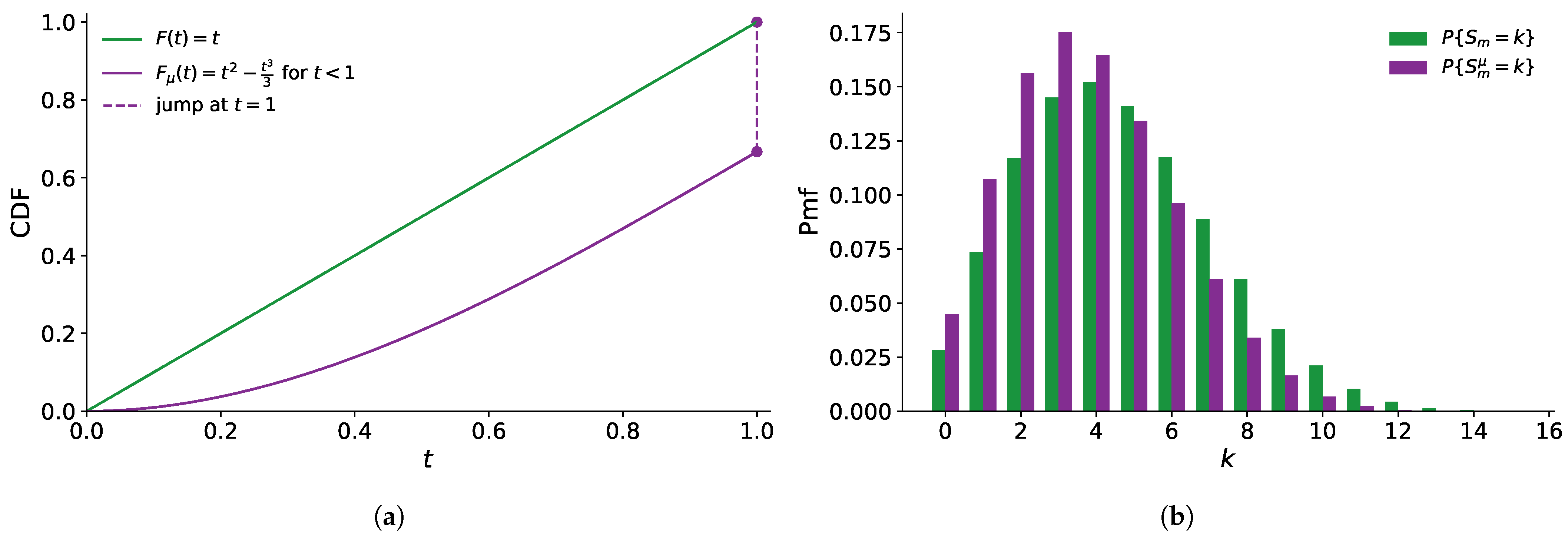
provides numerical estimates of these probabilities, comparing them against the ordinary values. Figure 2 visualizes why the exceedance-count distribution changes under fuzzification for the uniform cdf. On the left side, the fuzzy improved cdf $F_{\mu }\left(t\right)=t^2-\frac{t^3}{3}$ lies below the cdf $F\left(t\right)=t$ for $0<t<1$ and then jumps to 1 at $t=1$, since $F_{\mu }\left(1^{-}\right)=2/3$ and $P(X_{\mu }=1)=1/3$. Because the order statistic endpoint $X_{s:n}$ satisfies $X_{s:n}<1$ almost surely, this endpoint mass is not counted in the open interval $(X_{r:n},X_{s:n})$ and, therefore, reduces the effective inclusion probability $F_{\mu }\left(X_{s:n}\right)-F_{\mu }\left(X_{r:n}\right)$. The right side shows the resulting shift of probability mass in $S_m^{\mu }$ toward smaller counts compared to the ordinary $S_m$.

3.3. Exponential Distribution with Membership Function $\mu$ Defined via $g\left(x\right)=1-e^{-2x}$

Next, take the exponential cdf $F\left(x\right)=1-e^{-x}$ together with $g\left(u\right)=1-e^{-2u}$.

$$F_{\mu }\left(t\right)={\int }_0^t(1-e^{-2(t-x)})e^{-x}dx={(1-e^{-t})}^2.$$

where

$$\begin{array}{cc}\hfill P\{S_m^{\mu }=k\}=& {\displaystyle \frac{n!}{(r-1)!(s-r-1)!(n-s)!}}\left({\displaystyle \genfrac{}{}{0pt}{}{m}{k}}\right){\int }_0^{\infty }{\int }_u^{\infty }{\left[{(1-e^{-v})}^2-{(1-e^{-u})}^2\right]}^k\hfill \\ \hfill & \times {\left\{1-\left[{(1-e^{-v})}^2-{(1-e^{-u})}^2\right]\right\}}^{m-k}{e}^{-u}{e}^{-v}\hfill \\ & \times {\left(1-e^{-u}\right)}^{r-1}{\left(e^{-u}-e^{-v}\right)}^{s-r-1}{e}^{-v(n-s)}dvdu\hfill \end{array}$$

Table 3. Exponential cdf $F\left(x\right)=1-e^{-x}$ with $g\left(u\right)=1-e^{-2u}$ newcomer-count probabilities. Ordinary $S_m$ with newcomers from F. Fuzzy improved $S_m^{\mu }$ with newcomers from $F_{\mu }$.

n	r	s	k	m	$\mathit{P}\{{\mathit{S}}_{\mathit{m}}=\mathit{k}\}$	$\mathit{P}\{{\mathit{S}}_{\mathit{m}}^{\mathit{\mu }}=\mathit{k}\}$
12	6	10	4	15	0.15217391	0.12555307
12	5	9	5	18	0.13174951	0.11929091
12	5	10	2	14	0.07826087	0.05796734
10	4	9	1	12	0.03377428	0.02216934
10	4	9	3	16	0.05645613	0.03665205
8	5	7	3	10	0.15686275	0.16107528
8	2	3	4	9	0.03257919	0.01373167
6	3	5	2	8	0.20979021	0.19193057
8	1	7	1	11	0.00523934	0.02081188

reports the corresponding probabilities and compares them with the ordinary case.

The ordinary probabilities $P\{S_m=k\}$ are computed from the beta-binomial formula and are therefore exact up to numerical evaluation of beta functions. For numerical stability we evaluate beta ratios using log-beta functions (equivalently, $ln\mathsf{\Gamma }$).

For the fuzzy improved probabilities $P\{S_m^{\mu }=k\}$, no closed form is available in general, and the values reported and are obtained by numerical evaluation of the integral in Equation (10). On bounded supports (uniform cdf), we integrate over the triangular region $0<u<v<1$. On unbounded supports (exponential cdf), we use a change of variables that maps $(u,v)\in {(0,\infty )}^2$ with $u<v$ to a bounded triangular region, which improves numerical stability; for instance, one may set $x=e^{-u}$ and $y=e^{-v}$ so that $1>x>y>0$.

All integrals are evaluated by adaptive quadrature with user-specified absolute and relative tolerance. Reported probabilities are rounded to 8 decimal places. As internal checks, for each parameter set we verify that ${\sum }_{k=0}^{m}P\{S_m^{\mu }=k\}=1$ up to numerical error, and we confirm that the corresponding mean and variance computed from the pmf agree with the moment identities derived in Section 4 when applicable. Selected cases can additionally be cross-validated by Monte Carlo simulation of the two-sample case (generation of $(X_{r:n},X_{s:n})$ from F and newcomers from $F_{\mu }$) to ensure agreement within simulation error.

4. Asymptotic Distribution of the Newcomer Proportion

In this section, we adapt the exceedance-statistics framework of [14] to the newcomer problem. We treat, separately, the ordinary newcomer model ($Q:=F$) and the fuzzy improved newcomer model ($Q:=F_{\mu }$). For both cases, we give the finite-sample form for $S_m$, derive closed-form expressions for $E\left({\zeta }_m\right)$ and $\mathrm{Var}\left({\zeta }_m\right)$, and identify the large-m limit distribution of the proportion ${\zeta }_m=S_m/m$.

Let F be a cdf on $[a,b]$ with pdf f when it exists. Let $X_1,\dots ,X_n$ be iid random variables with cdf F on $[a,b]$. For any integrable $\phi :{\mathbb{R}}^n\to \mathbb{R}$ and the (linear) functional $H_F\left(\phi \right)$ in Section 2.1. Let $f_1,f_2:{\mathbb{R}}^n\to \mathbb{R}$ be measurable with $f_1\left(\overline{u}\right)\le f_2\left(\overline{u}\right)$. In our main application, $f_1\left(\overline{X}\right)=X_{r:n}$ and $f_2\left(\overline{X}\right)=X_{s:n}$ with $1\le r<s\le n$.

Let Equation (2) be the fuzzy ordering membership function, where g is nondecreasing with $g\left(0\right)=0$. The fuzzy improved cdf $F_{\mu }$ is defined in Equation (3). This is the single place where “fuzziness” enters; once F and g are introduced, $F_{\mu }$ is determined. Let $X_{n+1},\dots ,X_{n+m}$ be newcomers with cdf Q, independent of $(X_1,\dots ,X_n)$. For $k=1,\dots ,m$, define

$$A_k:=\{f_1\left(\overline{X}\right)<X_{n+k}<f_2\left(\overline{X}\right)\},{\xi }_k:=I\left\{A_k\right\}.$$

Then

$$p=P\left(A_k\right)=H_F\left\{Q\left(f_2\left(\overline{u}\right)\right)-Q\left(f_1\left(\overline{u}\right)\right)\right\}=:H_F\left\{Q_{f_1}^{f_2}\right\},$$

and, conditionally on $(X_1,\dots ,X_n)$, the variables ${\xi }_1,\dots ,{\xi }_m$ are independent Bernoulli with success probability $p\left(\overline{X}\right)=Q\left(f_2\left(\overline{X}\right)\right)-Q\left(f_1\left(\overline{X}\right)\right)$.

In the ordinary case, take $Q=F$ and write

$$S_m=\sum _{k=1}^m{\xi }_k,{\zeta }_m={\displaystyle \frac{S_m}{m}}.$$

In the fuzzy improved case, take $Q=F_{\mu }$ and write

$$S_m^{\mu }=\sum _{k=1}^m{\xi }_k^{\mu },{\zeta }_m^{\mu }={\displaystyle \frac{S_m^{\mu }}{m}},$$

where ${\xi }_k^{\mu }:=I\{f_1\left(\overline{X}\right)<X_{n+k}<f_2\left(\overline{X}\right)\}$ and $X_{n+1},\dots ,X_{n+m}$ are newcomers with cdf $F_{\mu }$, independent of $(X_1,\dots ,X_n)$. The limit cdf is

$$\begin{array}{c}\hfill C^{\mu }\left(x\right):=P\left\{{\left(F_{\mu }\right)}_{f_1}^{f_2}(X_1,\dots ,X_n)\le x\right\},0\le x\le 1.\end{array}$$

Then the uniform convergence holds:

$$\underset{0\le x\le 1}{sup}|P\{{\zeta }_m^{\mu }\le x\}-C^{\mu }\left(x\right)|⟶0.$$

Now take $f_1\left(\overline{X}\right)=X_{r:n}$ and $f_2\left(\overline{X}\right)=X_{s:n}$ with $1\le r<s\le n$. Set $U:=X_{r:n}$ and $V:=X_{s:n}$, and apply the probability integral transform

$$W:=F\left(U\right),Z:=F\left(V\right),0\le W\le Z\le 1.$$

(12)

Then $(W,Z)$ has joint density

$$f_{W,Z}(w,z)={\displaystyle \frac{n!}{(r-1)!(s-r-1)!(n-s)!}}{w}^{r-1}{(z-w)}^{s-r-1}{(1-z)}^{n-s},0\le w\le z\le 1,$$

which is distribution-free (it does not depend on F); see, e.g., [1,2].

Since F is continuous and strictly increasing on $(a,b)$, the inverse $F^{-1}$ exists and $U=F^{-1}\left(W\right)$, $V=F^{-1}\left(Z\right)$. Under the change of variables $(u,v)\mapsto (w,z)=\left(F\right(u),F(v\left)\right)$, the Jacobian contributes a factor $1/\left(f\right(u\left)f\right(v\left)\right)$, which cancels the $f\left(u\right)f\left(v\right)$ term in the joint density of $(U,V)$, yielding the distribution-free density of $(W,Z)$ above. Define $\phi \left(w\right):=F_{\mu }\left(F^{-1}\left(w\right)\right)$ and $p(w,z):=\phi \left(z\right)-\phi \left(w\right)$.

$$\phi \left(w\right):=F_{\mu }\left(F^{-1}\left(w\right)\right),p(w,z):=\phi \left(z\right)-\phi \left(w\right),0\le w\le z\le 1.$$

(13)

Then for $U=X_{r:n},V=X_{s:n}$ and $W=F\left(U\right),Z=F\left(V\right)$,

$$F_{\mu }\left(V\right)-F_{\mu }\left(U\right)=\phi \left(Z\right)-\phi \left(W\right).$$

(14)

If, in addition, F and $F_{\mu }$ are absolutely continuous with densities f and $f_{\mu }$, and if F is strictly increasing so that $f\left(F^{-1}\left(w\right)\right)>0$ on the region of interest, then by the chain rule on $(0,1)$

$${\phi }^{\prime }\left(w\right)={\displaystyle \frac{d}{dw}}{F}_{\mu }\left(F^{-1}\left(w\right)\right)={\displaystyle \frac{f_{\mu }\left(F^{-1}\left(w\right)\right)}{f\left(F^{-1}\left(w\right)\right)}}\ge 0.$$

When F and $F_{\mu }$ yield a closed-form $\phi \left(w\right)=F_{\mu }\left(F^{-1}\left(w\right)\right)$, sampling can be done directly on $[0,1]$ via $(W,Z)=\left(F\right(U),F(V\left)\right)$.

$$\begin{array}{cc}\hfill C^{\mu }\left(x\right)=& {\displaystyle \frac{n!}{(r-1)!(s-r-1)!(n-s)!}}{\int }_0^1{\int }_w^{1}I\{\phi \left(z\right)-\phi \left(w\right)\le x\}\hfill \\ \hfill & \times w^{r-1}{(z-w)}^{s-r-1}{(1-z)}^{n-s}dzdw.\hfill \end{array}$$

(15)

This reduces the inner integral in $C^{\mu }\left(x\right)$ to an incomplete beta function, yielding a single-integral representation. Because $\phi$ is nondecreasing, the set $\{z\in [w,1]:\phi (z)-\phi (w)\le x\}$ is an interval $[w,z_x\left(w\right)]$ with

$$z_x\left(w\right):=min\left\{1,{\phi }^{-1}(\phi \left(w\right)+x)\right\}.$$

(16)

Here ${\phi }^{-1}$ denotes the (right-continuous) generalized inverse of the nondecreasing $\phi$. So the inner integral is

$${\int }_w^{z_x\left(w\right)}{(z-w)}^{s-r-1}{(1-z)}^{n-s}dz.$$

Let $t=(z-w)/(1-w)\in [0,1]$, i.e., $z=w+(1-w)t$. Then $dz=(1-w)dt$ and

$$\begin{array}{c}\hfill z-w=(1-w)t,1-z=1-w-(1-w)t=(1-w)(1-t).\end{array}$$

Hence

$$\begin{array}{cc}\hfill {\int }_w^{z_x\left(w\right)}{(z-w)}^{s-r-1}{(1-z)}^{n-s}dz=& {\int }_0^{T_x\left(w\right)}{(1-w)}^{s-r-1}{t}^{s-r-1}{(1-w)}^{n-s}{(1-t)}^{n-s}(1-w)dt\hfill \\ \hfill =& {(1-w)}^{n-r}{\int }_0^{T_x\left(w\right)}{t}^{s-r-1}{(1-t)}^{n-s}dt\hfill \\ \hfill =& {(1-w)}^{n-r}{B}_{T_x\left(w\right)}(s-r,n-s+1),\hfill \end{array}$$

where $T_x\left(w\right):={\displaystyle \frac{z_x\left(w\right)-w}{1-w}}\in [0,1]$ and $B_y(a,b)={\int }_0^y{t}^{a-1}{(1-t)}^{b-1}dt$ is the (unregularized) incomplete beta, $B(a,b)$ is the beta function, and $I_y(a,b)=B_y(a,b)/B(a,b)$ is the regularized form. This yields single-integral form

$$\begin{array}{c}\hfill C^{\mu }\left(x\right)={\displaystyle \frac{n!}{(r-1)!(s-r-1)!(n-s)!}}{\int }_0^1{w}^{r-1}{(1-w)}^{n-r}{B}_{T_x\left(w\right)}(s-r,n-s+1)dw.\end{array}$$

(17)

Let $b_{\mu }:=E[\phi \left(Z\right)-\phi \left(W\right)]$ and $a_{\mu }:=E\left[{(\phi \left(Z\right)-\phi \left(W\right))}^2\right]$ under $f_{W,Z}$ above. Then

$$\begin{array}{cc}\hfill E\left({\zeta }_m^{\mu }\right)=& b_{\mu },\hfill \\ \hfill \mathrm{Var}\left({\zeta }_m^{\mu }\right)=& (a_{\mu }-b_{\mu }^2)-{\displaystyle \frac{a_{\mu }-b_{\mu }}{m}}.\hfill \end{array}$$

(18)

4.1. Uniform Cdf $F\left(x\right)$ on $[0,1]$ and $g\left(u\right)=1-{(1-u)}^{\lambda }$ Exact Pmf of $S_m^{\mu }$ and ${\zeta }_m^{\mu }$

$$\begin{array}{cc}\hfill F\left(x\right)=x,& f\left(x\right)=1;\hfill \\ \hfill g\left(u\right)=1-{(1-u)}^{\lambda }& ,0\le u\le 1.\hfill \end{array}$$

Then the fuzzy improved cdf for $\lambda =2$

$$\phi \left(w\right)=F_{\mu }\left(F^{-1}\left(w\right)\right)=\left\{\begin{array}{cc}{w}^2-{\displaystyle \frac{w^3}{3}},\hfill & 0\le w<1,\hfill \\ 1,\hfill & w=1.\hfill \end{array}\right.$$

For $0<u<v<1$, by Equation (10),

$$F_{\mu }\left(v\right)-F_{\mu }\left(u\right)=(v-u)\left[(v+u)-{\displaystyle \frac{1}{3}}(v^2+vu+u^2)\right].$$

To carry the fuzziness over to $[0,1]$, we compose with the inverse cdf and define, as in Equation (13),

$$\begin{array}{c}\hfill F_{\mu }\left(w\right)=w^2-{\displaystyle \frac{w^3}{3}},0\le w\le 1.\end{array}$$

$C^{\mu }\left(x\right)$ is the cdf induced by Equation (14) for the $(r,s)$ order statistics; see Equation (15). As an example of $(n,r,s,m)=(12,6,10,15)$, the full probability mass function is detailed in

Table 4. Uniform cdf $F\left(x\right)=x$ on $[0,1]$ with $g\left(u\right)=1-{(1-u)}^2$ pmf of the newcomer proportions ${\zeta }_m=S_m/m$ and ${\zeta }_m^{\mu }=S_m^{\mu }/m$ at $x=k/m$ for $(n,r,s,m)=(12,6,10,15)$.

k	$\mathit{P}\{{\mathit{\zeta }}_{\mathit{m}}=\mathit{k}/\mathit{m}\}$	$\mathit{P}\{{\mathit{\zeta }}_{\mathit{m}}^{\mathit{\mu }}=\mathit{k}/\mathit{m}\}$
0	0.02820513	0.04458938
1	0.07357860	0.10705654
2	0.11705686	0.15591558
3	0.14492754	0.17515897
4	0.15217391	0.16476446
5	0.14096110	0.13441961
6	0.11746758	0.09651538
7	0.08884103	0.06117956
8	0.06107821	0.03406690
9	0.03800422	0.01646785
10	0.02117378	0.00678095
11	0.01036479	0.00231304
12	0.00431866	0.00062715
13	0.00144962	0.00012660
14	0.00035205	0.00001690
15	0.00004694	0.00000112
Sum	1.000000	1.000000
Mean of ${\zeta }_m$	0.307692	0.253753

.

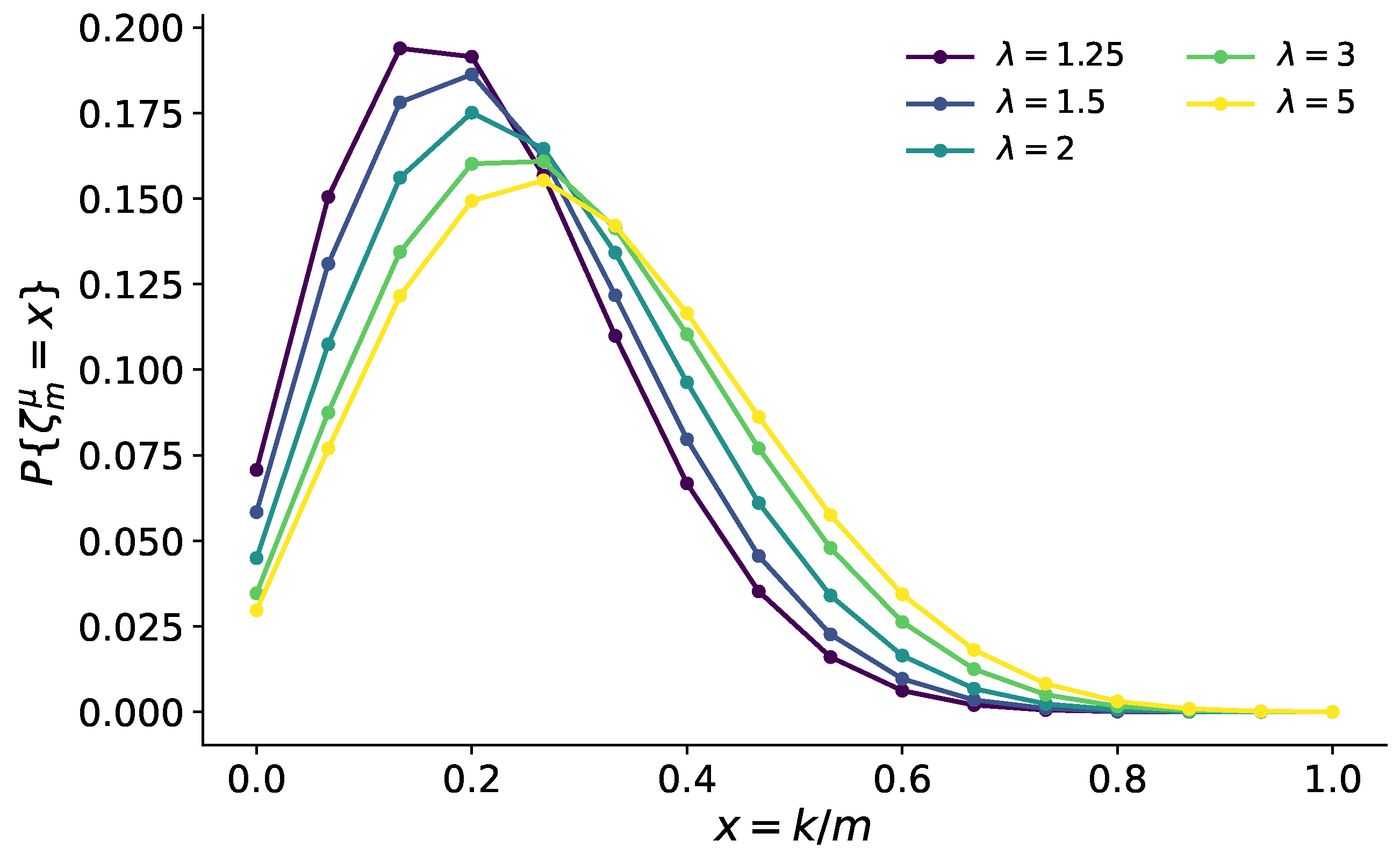
Figure 3 illustrates how the distribution of the fuzzy improved newcomer proportion ${\zeta }_m^{\mu }$ depends on the choice of the membership function g. Although the order statistic interval $(X_{r:n},X_{s:n})$ remains ordinary (and, hence, distribution-free under the probability integral transform), varying $\lambda$ changes the induced map Equation (13) and, therefore, changes the random inclusion probability Equation (14). As $\lambda$ increases, g becomes steeper, corresponding to a stronger graded notion of “$x{\le }_{\mu }t$” and leading to a systematic redistribution of probability mass across the grid values $k/m$. This sensitivity confirms that the fuzzification mechanism affects $S_m^{\mu }$ (and not only its mean), and it provides a practical handle for tuning the predictive behavior of exceedance proportions under boundary uncertainty.

4.2. Exponential Cdf $F\left(t\right)=1-e^{-t}$ and $g\left(u\right)=1-e^{-2u}$ Exact Pmf of $S_m^{\mu }$ and ${\zeta }_m^{\mu }$

We observe random variables $X_1,\dots ,X_n$ from the exponential cdf $F\left(x\right)=1-e^{-x}$. The membership function $\mu$ defined via $g\left(u\right)=1-e^{-2u}$ is non-negative and nondecreasing. Fuzzy improved cdf is

$$F_{\mu }\left(t\right)={\int }_0^t[1-e^{-2(t-x)}]e^{-x}dx={(1-e^{-t})}^2$$

from the Equation (3). We apply the probability integral transform $W=F\left(U\right)$, $Z=F\left(V\right)$. The Jacobian cancels $f\left(u\right)f\left(v\right)$, giving the pdf $0\le w\le z\le 1$ in Equation (11). To carry the fuzziness over to $[0,1]$, we compose with the inverse cdf and define Equation (13)

$$F^{-1}\left(w\right)=-ln(1-w).$$

Since $1-e^{-F^{-1}\left(w\right)}=1-(1-w)=w$, we obtain Equation (13)

$$\begin{array}{c}\hfill \phi \left(w\right)=w^2,\mathrm{hence}{F}_{\mu }\left(V\right)-F_{\mu }\left(U\right)=\phi \left(Z\right)-\phi \left(W\right)=Z^2-W^2.\end{array}$$

By definition, Equation (15),

$$\begin{array}{cc}\hfill C^{\mu }\left(x\right)=& P\{Z^2-W^2\le x\}={\displaystyle \frac{n!}{(r-1)!(s-r-1)!(n-s)!}}\hfill \\ \hfill & \times {\int }_0^1{\int }_w^{1}I\{z^2-w^2\le x\}{w}^{r-1}{(z-w)}^{s-r-1}{(1-z)}^{n-s}dzdw.\hfill \end{array}$$

For $w\in [0,1]$, $z^2-w^2\le x$ is $z\le z_x\left(w\right):=min\{1,\sqrt{x+w^2}\}$. Let $w_{*}=\sqrt{1-x}$. Then

$$\begin{array}{cc}\hfill C^{\mu }\left(x\right)={\displaystyle \frac{n!}{(r-1)!(s-r-1)!(n-s)!}}[& {\int }_0^{w_{*}}{w}^{r-1}{(1-w)}^{n-r}{B}_{T_x\left(w\right)}\left(s-r,n-s+1\right)dw\hfill \\ \hfill & +B\left(s-r,n-s+1\right){\int }_{w_{*}}^1{w}^{r-1}{(1-w)}^{n-r}dw],\hfill \end{array}$$

For w, substitute $t={\displaystyle \frac{z-w}{1-w}}$ so that $z=w+(1-w)t$ and $dz=(1-w)dt$. Then use the Equation (17) with $T\left(w\right)={\displaystyle \frac{z\left(w\right)-w}{1-w}}\in [0,1]$ where $B_y(a,b)={\int }_0^y{t}^{a-1}{(1-t)}^{b-1}dt$ is the incomplete beta and $I_y(a,b)=B_y(a,b)/B(a,b)$ is its regularized form. Taking $z\left(w\right)=z_x\left(w\right)=min\{1,\sqrt{x+w^2}\}$ gives

$$T_x\left(w\right)={\displaystyle \frac{min\{1,\sqrt{x+w^2}\}-w}{1-w}}\in [0,1].$$

The full pmf is in

Table 5. Exponential cdf $F\left(x\right)=1-e^{-x}$ with $g\left(u\right)=1-e^{-2u}$ pmf of the newcomer proportions ${\zeta }_m=S_m/m$ and ${\zeta }_m^{\mu }=S_m^{\mu }/m$ at $x=k/m$ for $(n,r,s,m)=(12,6,10,15)$.

k	$\mathit{P}\{{\mathit{\zeta }}_{\mathit{m}}=\mathit{k}/\mathit{m}\}$	$\mathit{P}\{{\mathit{\zeta }}_{\mathit{m}}^{\mathit{\mu }}=\mathit{k}/\mathit{m}\}$
0	0.02820513	0.01757589
1	0.07357860	0.04776665
2	0.11705686	0.08083733
3	0.14492754	0.10846365
4	0.15217391	0.12555307
5	0.14096110	0.13040067
6	0.11746758	0.12398360
7	0.08884103	0.10897001
8	0.06107821	0.08878801
9	0.03800422	0.06688322
10	0.02117378	0.04618430
11	0.01036479	0.02876719
12	0.00431866	0.01571451
13	0.00144962	0.00715837
14	0.00035205	0.00246099
15	0.00004694	0.00049255
Sum	1.000000	1.000000
Mean of ${\zeta }_m$	0.307692	0.373983

.

5. Results and Discussion

This section synthesizes the numerical findings from Section 3 (finite-sample pmfs) and Section 4 (limit distribution of the newcomer proportion). The ordinary case $Q=F$ is distribution-free for the interval $(X_{r:n},X_{s:n})$, whereas the fuzzy improved model $Q=F_{\mu }$ depends on the membership function $\mu$ through g and the induced mapping Equation (13).

A practical advantage of the representation is that the sampling variability of the order statistic interval is handled in a distribution-free manner through the probability integral transform Equation (12) whose joint density depends only on $(n,r,s)$ and not on the particular baseline cdf F. The effect of the fuzzy improved newcomer model enters only through the nondecreasing mapping Equation (13) so that the random inclusion probability is Equation (14). Consequently, once $\phi$ is available, both finite-sample exceedance counts and the large-m limit distribution can be evaluated without further distribution-specific order-statistic calculations.

For general choices of the baseline model F and membership function g, the functions $F_{\mu }$ and $\phi$ can be computed numerically by one-dimensional quadrature from the definition Equation (3) together with the monotone inversion $t=F^{-1}\left(w\right)$. In the finite-sample regime, the pmf of $S_m^{\mu }$ is obtained from the two-dimensional integral in Equation (10) and is responsive to adaptive quadrature after necessary changes of variables on unbounded supports. In the asymptotic form, the limit cdf $C^{\mu }$ in Equation (17) reduces evaluation to a one-dimensional integral once Equation (16) is computed via the generalized inverse of $\phi$. When rapid numerical assessment is needed, Monte Carlo evaluation is also straightforward: one may sample $(W,Z)$ directly from their distribution-free density and then compute Equation (14), yielding fast simulation-based approximations of $C^{\mu }$ and of the mixed-binomial distribution of $S_m^{\mu }$.

Table 1, Table 2, Table 3, Table 4 and Table 5 show that fuzzification can shift probability mass in non-uniform ways across k, even when $(n,r,s,m)$ are held fixed. In particular, the direction of the shift depends on both cdf F and the choice of g. For the bounded-support uniform cdf with $g\left(u\right)=1-{(1-u)}^2$, the induced $F_{\mu }$ has an endpoint atom at $t=1$, which can materially change the inclusion probability Equation (14) and, therefore, $S_m^{\mu }$. For the exponential parent with $g\left(u\right)=1-e^{-2u}$, the induced $F_{\mu }\left(t\right)={(1-e^{-t})}^2$ corresponds to a systematically different tail behavior than F, and the pmf of $S_m^{\mu }$ reflects this change. This mechanism is illustrated in Figure 2, where the jump of $F_{\mu }$ at the upper endpoint and the downward shift in the pmf of $S_m^{\mu }$ are shown side by side.

For $Q=F$, the inclusion probability $p=F\left(X_{s:n}\right)-F\left(X_{r:n}\right)$ has a $\mathrm{Beta}(s-r,n-s+r+1)$ distribution, so $E\left({\zeta }_m\right)=E\left(p\right)=(s-r)/(n+1)$. For the canonical parameter set $(n,r,s,m)=(12,6,10,15)$, this yields $E\left({\zeta }_m\right)=4/13\approx 0.307692$. In contrast, Equation (18) depends on $F_{\mu }$ (equivalently on g).

Table 6. Mean and variance of the newcomer proportion comparison for $(n,r,s,m)=(12,6,10,15)$ comparison using the full pmfs in Table 4 and Table 5.

Model	$\mathit{E}\left({\mathit{\zeta }}_{\mathit{m}}\right)$	$\mathbf{Var}\left({\mathit{\zeta }}_{\mathit{m}}\right)$
$Q=F$	0.307692	0.028402
Uniform cdf, $g\left(u\right)=1-{(1-u)}^2$	0.253753	0.021670
Exponential cdf, $g\left(u\right)=1-e^{-2u}$	0.373983	0.036511

summarizes the corresponding mean and variance of ${\zeta }_m$ and ${\zeta }_m^{\mu }$ for the two detailed pmf grids in Table 4 and Table 5. In the uniform example, fuzzification decreases both the mean and the variance of the proportion. In the exponential example with $g\left(u\right)=1-e^{-2u}$, fuzzification increases the mean and also increases dispersion.

Beyond mean and variance, the full pmfs show that fuzzification can substantially reshape tail risks at fixed $(n,r,s,m)$. For the canonical set $(n,r,s,m)=(12,6,10,15)$, the ordinary model gives $P(S_m\le 2)=0.218841$ and $P(S_m\ge 10)=0.037706$ from Table 4. Under the uniform fuzzification with an endpoint atom, the left tail increases to $P(S_m^{\mu }\le 2)=0.307562$ and the right tail decreases to $P(S_m^{\mu }\ge 10)=0.009866$ (Table 4), reflecting a pronounced shift of mass toward smaller counts. In contrast, under exponential fuzzification with $g\left(u\right)=1-e^{-2u}$, the left tail decreases to $P(S_m^{\mu }\le 2)=0.146180$ while the right tail increases to $P(S_m^{\mu }\ge 10)=0.100778$ (Table 5), indicating that in this case fuzzification makes large exceedance counts substantially more likely. These tail comparisons make explicit that fuzzification is not merely a variance adjustment:

Table 7. Tail-probability comparison for $(n,r,s,m)=(12,6,10,15)$ using the full pmfs in Table 4 and Table 5.

Model	$\mathit{P}({\mathit{S}}_{\mathit{m}}\le 2)$	$\mathit{P}({\mathit{S}}_{\mathit{m}}\ge 10)$
$Q=F$	0.218841	0.037706
Uniform cdf, $g\left(u\right)=1-{(1-u)}^2$	0.307562	0.009866
Exponential cdf, $g\left(u\right)=1-e^{-2u}$	0.146180	0.100778

shows it can reallocate probability mass asymmetrically, changing both low-count and high-count risk in a way that depends jointly on F and g.

The real-data tire illustration in Section 6.1 further reinforces this point by providing a data-driven setting in which F is fitted under censoring and $g(x;\theta )$ is estimated from data. For $(n,r,s,m)=(34,12,23,20)$, Tables 8 and 9 shows that the fuzzy improved newcomer model (with $\widehat{\theta }=12$) concentrates strongly near small counts: $P(S_m^{\mu }\le 2)=0.606650$ and $P(S_m^{\mu }\ge 10)=0.000050$, while the ordinary benchmark has $P(S_m\le 2)=0.059786$ and $P(S_m\ge 10)=0.111384$. Thus, in this application the calibrated fuzzification mechanism yields a markedly more conservative exceedance-count prediction, consistent with the interpretation that boundary uncertainty can reduce effective inclusion probabilities on a bounded working scale. The sensitivity analysis in Table 10 shows that this conservatism is tunable through $\theta$, with both $E\left({\zeta }_m^{\mu }\right)$ and $\mathrm{Var}\left({\zeta }_m^{\mu }\right)$ increasing as g becomes steeper and the endpoint mass $1-F_{\mu }\left(1^{-}\right)$ decreases.

Although Section 4 characterizes the large-m limit of ${\zeta }_m^{\mu }$, the asymptotic results are also informative for moderate newcomer sizes because $S_m^{\mu }$ is a binomial mixture for every finite m. Conditionally on the order-statistic sample, $S_m^{\mu }\mid (X_{r:n},X_{s:n})$ is binomial with success probability given by Equation (14); unconditionally, the distribution is obtained by mixing over the random inclusion probability induced by Equation (13). The limit law describes the mixing distribution of Equation (14), and finite-m effects arise only through binomial sampling noise around Equation (14). This separation is quantified by the exact variance identity in Equation (18), where the m-dependent term is $(a_{\mu }-b_{\mu })/m$; hence, the discrepancy between the finite-sample dispersion of ${\zeta }_m^{\mu }$ and the limit dispersion decays at rate $1/m$. In practice, for moderate m (as in our tables), one may compute the exact pmf via Equation (10) or use distribution-free Monte Carlo sampling of $(W,Z)$ to approximate the mixture, while $C^{\mu }$ provides a fast approximation and a direct description of how fuzzification reshapes the random inclusion probability Equation (14).

The numerical results support the following interpretation. The $Q=F$ reflects sampling variability of the order statistic interval only. The fuzzy improved model $Q=F_{\mu }$ alters the newcomer-generating mechanism via the graded comparison encoded in g, and the resulting distribution can exhibit either a reduction or an increase in predictive dispersion depending on how g reshapes F (including the appearance of boundary mass on bounded supports). Consequently, fuzzification should be viewed as a modeling choice that can materially change both the center and the spread of exceedance predictions, rather than as a purely “variance-inflating” perturbation.

6. Illustrative Applications

We illustrate how the proposed fuzzy-improved framework can be used in three complementary ways. First, we give a real reliability illustration for tire lifetimes, where the baseline model is an ordinary cdf F fitted to censored data and the fuzzification strength in the membership function $\mu$ is estimated from the same dataset; we then translate the fitted fuzzy improved model into exceedance-count predictions for an ordinary order statistic interval. Second, we describe a spam-filtering setting to clarify how graded thresholding and ranking can be formulated through the same membership function Equation (2), depending on whether fuzziness enters through re-measurement, decision softening, or pairwise ranking (Types 1–3). Third, we include a short parts-versus-systems example to emphasize that the same order statistic interval can support different operational decisions depending on whether newcomers represent component-level lifetimes (F) or system-level lifetimes induced by a fuzzy improved model ($F_{\mu }$). Throughout, $F_{\mu }$ denotes the fuzzy improved distribution function induced by $\mu$ as in Equation (3); the goal of these examples is to clarify how fuzzification enters the ordering and how it changes exceedance-count predictions in concrete applications.

6.1. Tire Lifetime (Reliability Planning with Parameter Estimation and Sensitivity)

We illustrate the proposed exceedance-count framework on a right-censored tire lifetime dataset [22]. Let T denote lifetime and let $n=34$ observations be available, with 11 observed failures and 23 right-censored values. The goal is to compare ordinary exceedance predictions with fuzzy improved newcomer predictions for the same order-statistic interval constructed from the initial sample. We follow fuzzy-set-based reliability reasoning as in [11], and use fuzzification to represent boundary uncertainty on a bounded working scale; see also standard reliability treatments [15,16,18].

6.1.1. Baseline Model and Ordinary Benchmark

We first fit a Weibull model to the censored lifetimes by maximum likelihood [21,23]. The baseline cdf on the T-scale is

$$F_T\left(t\right)=1-exp\left\{-{\left({\displaystyle \frac{t}{\alpha }}\right)}^{\beta }\right\},t>0.$$

and the MLEs for this dataset are

$$\widehat{\beta }=8.695568,\widehat{\alpha }=1.226089.$$

We take $(n,r,s,m)=(34,12,23,20)$ so that $s-r=11$. In the ordinary distribution-free benchmark ($Q=F_T$) for the invariant interval $(T_{r:n},T_{s:n})$, Equation (1) yields

$$E\left({\zeta }_m\right)={\displaystyle \frac{s-r}{n+1}}={\displaystyle \frac{11}{35}}=0.314286,$$

and the corresponding variance computed from the beta-binomial law is

$$\mathrm{Var}\left({\zeta }_m\right)=0.016463.$$

6.1.2. Bounded-Support Fuzzification and the Jump at the Boundary

As discussed in Section 2.2, on bounded supports the fuzzy improved cdf can exhibit a jump at the upper endpoint. To make this mechanism explicit in the tire illustration, we map lifetimes to the bounded interval $[0,1)$ via the monotone transform.

$$X={\displaystyle \frac{T}{T+c}},c=\widehat{\alpha }=1.226089.$$

This transformation preserves order and, therefore, preserves the order statistic interval in the sense that the events $\{T_{r:n}<T_{n+i}<T_{s:n}\}$ on the T-scale correspond exactly to $\{X_{r:n}<X_{n+i}<X_{s:n}\}$ on the X-scale.

Let $F_X$ denote the cdf of X induced by the fitted baseline $F_T$. Since the transform is monotone and $T=cx/(1-x)$, we have

$$F_X\left(x\right)=P(X\le x)=F_T\left({\displaystyle \frac{cx}{1-x}}\right),0<x<1.$$

On $[0,1]$ we use a membership function $\mu (x,t)=g(t-x)I\{t\ge x\}$ with a normalized exponential kernel

$$g(u;\theta )={\displaystyle \frac{1-e^{-\theta u}}{1-e^{-\theta }}},0\le u\le 1,\theta >0,$$

so that $g(0;\theta )=0$ and $g(1;\theta )=1$, consistent with the bounded-support conditions in Section 2.2. The fuzzy improved cdf on X is then

$$F_{\mu }\left(t\right)=\left\{\begin{array}{cc}0,\hfill & t\le 0,\hfill \\ {\displaystyle {\int }_0^{t}g(t-x;\theta )d{F}_X\left(x\right),}\hfill & 0<t<1,\hfill \\ 1,\hfill & t\ge 1,\hfill \end{array}\right.$$

and the corresponding left limit at the upper endpoint is

$$F_{\mu }\left(1^{-}\right)=\underset{t\to 1}{lim}{\int }_0^{t}g(t-x;\theta )d{F}_X\left(x\right),$$

which can be strictly less than 1. The boundary mass is, therefore

$$P\{X_{\mu }=1\}=1-F_{\mu }\left(1^{-}\right).$$

For the fitted tire example (reported below), we obtain

$$1-F_{\mu }\left(1^{-}\right)\approx 2.205343\times {10}^{-3}.$$

6.1.3. Estimation of the Fuzziness Parameter Under Censoring

Let $t_i$ be the observed time and let ${\delta }_i=1$ indicate an observed failure and ${\delta }_i=0$ indicate right censoring. Set

$$x_i={\displaystyle \frac{t_i}{t_i+c}}.$$

Assuming absolute continuity on $(0,1)$, the fuzzy improved density on the X satisfies the general identity in Equation (5):

$$f_{\mu }\left(t\right)={\int }_0^t{g}^{\prime }(t-x;\theta )f_X\left(x\right)dx,0<t<1,$$

with

$$g^{\prime }(u;\theta )={\displaystyle \frac{\theta e^{-\theta u}}{1-e^{-\theta }}},0<u<1.$$

We estimate $\theta$ by maximizing the standard right-censored log-likelihood under $F_{\mu }$:

$$\ell \left(\theta \right)=\sum _{i:{\delta }_i=1}ln{f}_{\mu }(x_i;\theta )+\sum _{i:{\delta }_i=0}ln\{1-F_{\mu }(x_i;\theta )\}.$$

To prevent extremely steep (nearly crisp) membership functions and to stabilize computation, we cap $\theta$ and maximize over $\theta \in (0,12]$. For this dataset the likelihood increases up to the cap; so

$$\widehat{\theta }=12.0,$$

attaining the imposed upper bound. The fitted baseline and fuzziness quantities are summarized in

Table 8. Tire data: Weibull baseline fit and bounded-support fuzzification (MLE $\widehat{\theta }$ and endpoint jump mass).

Baseline	$\widehat{\mathit{\beta }}$	$\widehat{\mathit{\alpha }}$	c	$\widehat{\mathit{\theta }}$	logLik	$1-{\mathit{F}}_{\mathit{\mu }}\left(1^{-}\right)$
Weibull	8.695568	1.226089	1.226089	12.0	−2.934650	2.205343 $\times {10}^{-3}$

.

6.1.4. Exceedance Counts for Ordinary and Fuzzy Improved Newcomers

We next compare exceedance-count distributions for the ordinary newcomer model and the fuzzy improved newcomer model on the bounded X. Let $X_1,\dots ,X_n$ denote the transformed initial sample and let $X_{1:n}\le \cdots \le X_{n:n}$ be the corresponding order statistics. The order statistic interval is $(X_{r:n},X_{s:n})$ with $(n,r,s,m)=(34,12,23,20)$.

For $m=20$ independent newcomers, define the ordinary benchmark with ${\tilde{X}}_1,\dots ,{\tilde{X}}_m$ iid $F_X$ and the fuzzy model with ${\tilde{X}}_1^{\mu },\dots ,{\tilde{X}}_m^{\mu }$ iid $F_{\mu }$, both samples independent of $(X_1,\dots ,X_n)$:

$$S_m=\sum _{i=1}^{m}I\{X_{r:n}<{\tilde{X}}_i<X_{s:n}\},S_m^{\mu }=\sum _{i=1}^{m}I\{X_{r:n}<{\tilde{X}}_i^{\mu }<X_{s:n}\}.$$

Write ${\zeta }_m=S_m/m$ and ${\zeta }_m^{\mu }=S_m^{\mu }/m$.

Table 9. Tire data: pmf of newcomer proportion ${\zeta }_m=S_m/m$ (ordinary) vs. ${\zeta }_m^{\mu }=S_m^{\mu }/m$ (fuzzy improved) for $(n,r,s,m)=(34,12,23,20)$.

k	$\mathit{P}\{{\mathit{\zeta }}_{\mathit{m}}=\mathit{k}/\mathit{m}\}$	$\mathit{P}\{{\mathit{\zeta }}_{\mathit{m}}^{\mathit{\mu }}=\mathit{k}/\mathit{m}\}$
0	0.002988814	0.111066667
1	0.015291600	0.236116667
2	0.041505780	0.259466667
3	0.078962220	0.197266667
4	0.117456300	0.112600000
5	0.144561600	0.052650000
6	0.152170100	0.021483333
7	0.139832000	0.006716667
8	0.113613500	0.002233333
9	0.082234530	0.000350000
10	0.053210580	0.000033333
11	0.030782980	0.000016667
12	0.015872470	0.000000000
13	0.007246985	0.000000000
14	0.002898794	0.000000000
15	0.000999584	0.000000000
16	0.000290058	0.000000000
17	0.000068249	0.000000000
18	0.000012250	0.000000000
19	0.000001496	0.000000000
20	0.000000093	0.000000000
Sum	1.000000	1.000000

reports the pmf values on the grid $x=k/m$, comparing the ordinary proportion ${\zeta }_m$ with the fuzzy improved proportion ${\zeta }_m^{\mu }$.

From Table 9, fuzzification shifts probability mass strongly toward smaller exceedance proportions. The summary moments are

$$E\left({\zeta }_m\right)=0.314286,\mathrm{Var}\left({\zeta }_m\right)=0.016463,$$

and

$$E\left({\zeta }_m^{\mu }\right)=0.112898,\mathrm{Var}\left({\zeta }_m^{\mu }\right)=0.005870.$$

In addition, the distribution is concentrated near the lower grid values; for example

$$P(S_m^{\mu }\le 2)=0.606650,P(S_m^{\mu }\ge 10)=0.000050.$$

6.1.5. Sensitivity in $\theta$ and the Boundary Mass

Finally,

Table 10. Tire data: sensitivity of ${\zeta }_m^{\mu }$ to the fuzziness parameter $\theta$ (moments, tail probabilities, and endpoint jump mass).

$\mathit{\theta }$	$\mathit{E}\left({\mathit{\zeta }}_{\mathit{m}}^{\mathit{\mu }}\right)$	$\mathbf{Var}\left({\mathit{\zeta }}_{\mathit{m}}^{\mathit{\mu }}\right)$	$\mathit{P}({\mathit{S}}_{\mathit{m}}^{\mathit{\mu }}\le 2)$	$\mathit{P}({\mathit{S}}_{\mathit{m}}^{\mathit{\mu }}\ge 10)$	$1-{\mathit{F}}_{\mathit{\mu }}\left(1^{-}\right)$
6.0	0.066591	0.00342	0.847500	0.000000	0.043755
9.0	0.091647	0.00475	0.718683	0.000017	0.009933
12.0	0.112898	0.00587	0.606650	0.000050	0.002205

reports a sensitivity check for $\theta \in \{6,9,12\}$ under the same fitted baseline and the same order statistic interval. The last column reports the induced jump mass $1-F_{\mu }\left(1^{-}\right)$, which decreases as $\theta$ increases.

These computations illustrate two features emphasized in Section 2.2 and Section 4. First, the order statistic interval remains an ordinary order statistic interval on the working scale; in this case $(X_{r:n},X_{s:n})$. Thus, the randomness in $S_m^{\mu }$ arises through the same random endpoints as in the ordinary case. Second, fuzzification enters only through the newcomer distribution $F_{\mu }$ induced by g, and on bounded supports the induced endpoint mass can reduce the effective inclusion probability $F_{\mu }\left(X_{s:n}\right)-F_{\mu }\left(X_{r:n}\right)$, shifting the distribution of $S_m^{\mu }$ toward smaller counts.

6.2. Spam Filtering (Ranking and Thresholding)

Our framing mirrors standard text categorization, ROC evaluation, and spam-filtering practice [24,25,26,27]. Let $S\in [0,1]$ be a spam score (the larger, the more spam-like), and define haminess $H=1-S\in [0,1]$ so that smaller H indicates more spam-like content. Choose a membership function $\mu$ (via g) for the fuzzy decision event $H{\le }_{\mu }t$:

$$g\left(u\right)={\displaystyle \frac{1-e^{-\alpha u}}{1-e^{-\alpha }}},0\le u\le 1,\alpha >0,$$

and model H with cdf F on $[0,1]$ (e.g., Beta). This graded-threshold formulation supports soft decisions near the boundary [24].

6.2.1. Type 1 (Re-Measure, Then Rank)

Construct

$$F_{\mu }\left(t\right)={\int }_0^{t}g(t-h)dF\left(h\right),F_{X_{r:n}}\left(t\right)=I_{F_{\mu }\left(t\right)}(r,n-r+1).$$

Rank emails by $X_{1:n}\le \cdots \le X_{n:n}$ to form a soft top-k spam list (smaller X is more spam-like). This suggests A/B testing graded thresholds in inbox triage, with $\alpha$ tuning aggressiveness.

6.2.2. Type 2 (Ordinary Order, Fuzzy Decision)

Compute the ordinary r-th smallest haminess $H_{r:n}$ and evaluate $F_{[r:n]}\left(t\right)$ via Equation (8). This yields graded thresholds for moderation queues (“quarantine if $H{\le }_{\mu }t$”), reducing flips near the boundary.

6.2.3. Type 3 (Fuzzy Pairwise Ranking)

With $\mu (h_i,h_j)=g(h_j-h_i)I\{h_j\ge h_i\}$, the distribution of the fuzzy r-th rank $H^{\left(r\right)}$ follows from Equation (9) after substituting the cdf of H on $[0,1]$. Fuzzy pairwise grades can also provide an audit trail when scores are nearly tied.

Table 11. Task-type mapping for the three fuzzy order statistics formulations (Types 1–3). A checkmark indicates the recommended formulation for the task.

Task	Type 1	Type 2	Type 3
Re-measure items on a soft scale before ranking	✓
Preserve ordinary ordering; soften the decision rule		✓
Make the ranking itself robust to near ties			✓

summarizes when to use each of the three types of fuzzy order statistics.

6.3. Illustrative Case: Parts vs. Systems Under Ordinary and Fuzzy Models

We illustrate the practical difference between parts-level (ordinary) and system-level newcomer modeling in a fleet-maintenance setting. Assume controller lifetimes follow an exponential cdf $F\left(t\right)=1-e^{-t}$, $t\ge 0$. From an initial cohort of $n=12$ units with ordered failures $X_{1:12}\le \cdots \le X_{12:12}$, the analysis focuses on the order statistic interval $(X_{6:12},X_{10:12})$. The parts-level question is: what is the probability that a fresh controller lifetime falls in $(X_{6:12},X_{10:12})$? For iid lifetimes with cdf F, a single newcomer Y with cdf F satisfies the distribution-free identity

$$P\{X_{6:12}<Y<X_{10:12}\}={\displaystyle \frac{10-6}{12+1}}={\displaystyle \frac{4}{13}}.$$

For m newcomers, conditional on the order statistics interval

$$S_m\mid (X_{6:12},X_{10:12})\mathrm{is}\mathrm{binomial}\mathrm{with}\mathrm{parameters}\mathrm{Bin}\left(m,F\left(X_{10:12}\right)-F\left(X_{6:12}\right)\right),$$

but, unconditionally, $S_m$ is mixed binomial with a random success probability, with extra dispersion induced by the random interval. System behavior can differ materially [15,16]. If each unit has active redundancy (two controllers in parallel) and mission loss occurs only after both controllers fail, then a fuzzy ordering with $g\left(x\right)=1-e^{-2x}$ induces the fuzzy improved newcomer cdf

$$F_{\mu }\left(t\right)={\int }_0^t\left(1-e^{-2(t-x)}\right)e^{-x}dx={(1-e^{-t})}^2=F{\left(t\right)}^2,$$

which coincides with the lifetime distribution of a two-component parallel system (the maximum of two iid $\mathrm{Exp}\left(1\right)$ lifetimes). Relative to the parts-level model, this changes the random inclusion probability from $F\left(V\right)-F\left(U\right)$ to Equation (14) (with $U=X_{6:12}$, $V=X_{10:12}$) and, therefore, changes the entire distribution of $S_m$ over $(X_{6:12},X_{10:12})$.

Parts planning (ordinary) remains appropriate for replenishing individual controllers and routine technician scheduling, because it targets single-component lifetimes. In contrast, outage risk and service-level decisions should be anchored on the system-level newcomer model: thresholds may be set later, staffing and inventory policies may require buffers for both low and high realizations of $S_m$, and monitoring can escalate after the first failure to focus on the second-stage hazard that governs mission loss. This example highlights how the same interval $(X_{6:12},X_{10:12})$ can support distinct operational decisions depending on whether newcomers represent component lifetimes (F) or system lifetimes ($F_{\mu }$).

7. Conclusions

This paper establishes a two-sample exceedance-count framework in which the order statistic interval remains the classical invariant interval $(X_{r:n},X_{s:n})$ from an iid baseline sample with cdf F, while boundary uncertainty is represented through a fuzzy improved newcomer model with cdf $F_{\mu }$. The central methodological point is that fuzziness enters only through the graded comparison mechanism $\mu (x,t)$ (via g) and therefore only through the induced quantile-scale map $\phi \left(w\right)=F_{\mu }\left(F^{-1}\left(w\right)\right)$ in Equation (13). This separation preserves the distribution-free structure of the random interval via the probability integral transform $(W,Z)=(F\left(X_{r:n}\right),F\left(X_{s:n}\right))$ and isolates how the membership function reshapes newcomer inclusion probabilities through Equation (14).

Our theoretical results show that both the ordinary exceedance count $S_m$ (with $Q=F$) and the fuzzy exceedance count $S_m^{\mu }$ (with $Q=F_{\mu }$) are conditionally binomial given $(X_{r:n},X_{s:n})$, but differ in their unconditional mixing distributions. In the ordinary benchmark, the inclusion probability is beta-distributed and $S_m$ is beta-binomial. In the fuzzy improved model, the unconditional law remains a mixed binomial with mixing induced by $F_{\mu }$, yielding the exact finite-sample representation in Equation (10). For large newcomer sizes, we derived a distribution-free limit cdf $C^{\mu }$ (Equations (15)–(17)) and explicit moment expressions for ${\zeta }_m^{\mu }=S_m^{\mu }/m$ in Equation (18), clarifying how finite-m dispersion differs from the mixing variability.

The numerical and data analyses support two substantive conclusions that go beyond a change in variance. First, fuzzification can shift the entire exceedance-count distribution in ways that depend jointly on F and g. In the uniform bounded-support example, the endpoint jump in $F_{\mu }$ reduces effective inclusion probabilities and pushes mass toward smaller counts, whereas in the exponential example with $g\left(u\right)=1-e^{-2u}$ the resulting $F_{\mu }$ can increase the probability of larger counts. Second, these changes can be practically material. The tail-probability comparisons in Section 5 show that fuzzification may either amplify or dampen low-count and high-count risk, and the tire-life illustration in Section 6.1 demonstrates that a calibrated bounded-support fuzzification can yield markedly more conservative exceedance predictions, with sensitivity to the fuzziness parameter $\theta$ aligned with changes in the endpoint mass $1-F_{\mu }\left(1^{-}\right)$.

There are several future directions for extending the present framework. First, exceedance counts can be studied when the order statistic interval endpoints are also fuzzified (for example, using Type 1 or Type 2 constructions in Section 2.4), so that fuzziness in the interval and fuzziness in the newcomer mechanism are modeled jointly. Second, inference for $g(·;\theta )$ can be strengthened beyond point estimation under censoring by developing uncertainty quantification for exceedance functionals (e.g., tail probabilities of $S_m^{\mu }$) and propagating uncertainty in $(\theta ,\psi )$ into predictive statements. Third, allowing g (or $\theta$) to vary over time would capture drift in operational thresholds and can be represented through time-indexed versions of $\phi$ in Equation (13). Finally, multivariate extensions would support screening and classification settings where exceedance is defined by compound rules on several scores, while still leveraging the separation between the distribution-free order statistic interval and the fuzzified newcomer mechanism.

References

1. Arnold, B.C.; Balakrishnan, N.; Nagaraja, H.N. A First Course in Order Statistics; SIAM: Philadelphia, PA, USA, 2008. [Google Scholar] [CrossRef] [Scilit]
2. David, H.A.; Nagaraja, H.N. Order Statistics, 3rd ed.; Wiley: Hoboken, NJ, USA, 2003. [Google Scholar] [CrossRef] [Scilit]
3. Bairamov, I.G.; Kotz, S. On distributions of exceedances associated with order statistics and record values for arbitrary distributions. Stat. Pap. 2001, 42, 171–185. [Google Scholar] [CrossRef] [Scilit]
4. Asadi, M.; Bayramoglu, I. The mean residual life function of a k-out-of-n structure at the system level. IEEE Trans. Reliab. 2006, 55, 314–318. [Google Scholar] [CrossRef] [Scilit]
5. Eryılmaz, S. Reliability properties of consecutive k-out-of-n systems of arbitrarily dependent components. Reliab. Eng. Syst. Saf. 2009, 94, 350–356. [Google Scholar] [CrossRef] [Scilit]
6. Zadeh, L.A. Fuzzy sets. Inf. Control 1965, 8, 338–353. [Google Scholar] [CrossRef] [Scilit]
7. Puri, M.L.; Ralescu, D.A. Fuzzy random variables. J. Math. Anal. Appl. 1986, 114, 409–422. [Google Scholar] [CrossRef] [Scilit]
8. Couso, I.; Dubois, D. A perspective on the extension of stochastic orderings to fuzzy random variables. In Proceedings of IFSA–EUSFLAT 2015; Atlantis Press: Asturias, Spain, 2015; pp. 1003–1008. [Google Scholar] [CrossRef] [Scilit]
9. Bastani, F.B.; Chen, I.-R.; Tsao, T. Reliability of systems with fuzzy-failure criterion. In Proceedings of the Annual Reliability and Maintainability Symposium (RAMS), Anaheim, CA, USA, 24–27 January 1994; IEEE: Anaheim, CA, USA, 1994; pp. 442–448. [Google Scholar] [CrossRef] [Scilit]
10. Bowles, J.B.; Peláez, C.E. Fuzzy logic prioritization of failures in a system failure mode, effects and criticality analysis. Reliab. Eng. Syst. Saf. 1995, 50, 203–213. [Google Scholar] [CrossRef] [Scilit]
11. Kabir, S.; Papadopoulos, Y. Applications of fuzzy logic in safety and reliability engineering. Int. J. Approx. Reason. 2018, 100, 29–55. [Google Scholar] [CrossRef] [Scilit]
12. Leuschen, M.L.; Walker, I.D.; Cavallaro, J.R. Robot reliability using fuzzy fault trees and Markov models. In Sensor Fusion and Distributed Robotic Agents; (Proc. SPIE, Vol. 2905); Schenker, P.S., McKee, G.T., Eds.; SPIE: Bellingham, WA, USA, 1996; pp. 73–91. [Google Scholar] [CrossRef] [Scilit]
13. Bayramoglu, I. Fuzzy improved distribution function and fuzzy order statistics. J. Comput. Appl. Math. 2022, 411, 114266. [Google Scholar] [CrossRef] [Scilit]
14. Bairamov, I.G.; Gebizlioglu, O.L.; Kaya, M.F. Asymptotic distributions of statistics based on order statistics and record values and invariant confidence intervals. In Asymptotic Methods in Probability and Statistics with Applications; Balakrishnan, N., Ibragimov, I.A., Nevzorov, V.B., Eds.; Birkhauser: Boston, MA, USA, 2001; pp. 309–320. [Google Scholar] [CrossRef] [Scilit]
15. Rausand, M.; Høyland, A. System Reliability Theory: Models, Statistical Methods, and Applications, 2nd ed.; Wiley: Hoboken, NJ, USA, 2004; ISBN 978-0471471332. [Google Scholar]
16. Samaniego, F.J. System Signatures and Their Applications in Engineering Reliability; Springer: New York, NY, USA, 2007. [Google Scholar] [CrossRef] [Scilit]
17. Bairamov, I.; Arnold, B.C. On the residual lifelengths of the remaining components in an nk + 1 out of n system. Stat. Probab. Lett. 2008, 78, 945–952. [Google Scholar] [CrossRef] [Scilit]
18. Barlow, R.E.; Proschan, F. Statistical Theory of Reliability and Life Testing: Probability Models; Holt, Rinehart and Winston: New York, NY, USA, 1975; ISBN 978-0030858536. [Google Scholar]
19. Bairamov, I.G.; Petunin, Y. Structure of invariant confidence intervals containing the main distributed mass. Theory Probab. Appl. 1991, 35, 15–26. [Google Scholar] [CrossRef] [Scilit]
20. Casella, G.; Berger, R. Statistical Inference, 2nd ed.; Chapman and Hall/CRC: Boca Raton, FL, USA, 2024. [Google Scholar] [CrossRef] [Scilit]
21. Bedford, T.; Cooke, R.M. Probabilistic Risk Analysis: Foundations and Methods; Cambridge University Press: Cambridge, UK, 2001; ISBN 978-0-521-77320-1. [Google Scholar]
22. Meeker, W.Q. SMRD2Data: Data Sets Used in Statistical Methods for Reliability Data, 2nd ed.; Iowa State University: Ames, IA, USA; GitHub: San Francisco, CA, USA, 2021; Available online: https://github.com/wqmeeker/SMRD2Data (accessed on 2 February 2026).
23. Lawless, J.F. Statistical Models and Methods for Lifetime Data, 2nd ed.; Wiley: Hoboken, NJ, USA, 2003; ISBN 978-0-471-37215-8. [Google Scholar]
24. Fawcett, T. An introduction to ROC analysis. Pattern Recognit. Lett. 2006, 27, 861–874. [Google Scholar] [CrossRef] [Scilit]
25. Cormack, G.V. Email spam filtering: A systematic review. Found. Trends Inf. Retr. 2008, 1, 335–455. [Google Scholar] [CrossRef] [Scilit]
26. Sebastiani, F. Machine learning in automated text categorization. ACM Comput. Surv. 2002, 34, 47. [Google Scholar] [CrossRef] [Scilit]
27. Shehzad, F.; Rehman, A.; Javed, K.; Alnowibet, K.A.; Babri, H.A.; Rauf, H.T. Binned Term Count: An Alternative to Term Frequency for Text Categorization. Mathematics 2022, 10, 4124. [Google Scholar] [CrossRef] [Scilit]
Figure 1. Order statistic interval ( X r : n , X s : n ) from the iid sample X 1 , , X n and independent newcomers X n + 1 , , X n + m from the cdf F. Newcomers falling in the interval contribute to S m = i = 1 m I { X r : n < X n + i < X s : n } .
Mathematics 14 00627 g001
Figure 2. (a) Cdf comparison F vs. fuzzy improved F μ ; (b) Exceedance-count distributions S m vs. S m μ .
Mathematics 14 00627 g002
Figure 3. Uniform cdf F ( x ) = x on [ 0 , 1 ] : sensitivity of the fuzzy improved newcomer proportion ζ m μ = S m μ / m to the membership function g ( u ) = 1 ( 1 u ) λ , 0 u 1 , for ( n , r , s , m ) = ( 12 , 6 , 10 , 15 ) . The curves show the pmf of ζ m μ on the grid x = k / m , k = 0 , 1 , , m .
Mathematics 14 00627 g003