DISPEL-GNN: De-Illusion via Spectral Stability and Perturbation Bound-Enforced Learning for Community Detection with Risk-Aware Dynamic Attention in Graph Neural Networks

Abstract

Community detection in graphs can be viewed as the estimation of a partition map that remains stable under admissible perturbations of graph topology and node attributes. While modern graph neural networks (GNNs) achieve strong empirical accuracy, they often exhibit severe assignment drift under minor perturbations, leading to illusory community structures. In this work, we propose DISPEL-GNN, a stability-aware graph learning framework that integrates spectral operator regularization, Bayesian uncertainty modeling, and risk-aware dynamic attention for perturbation-bounded community detection. The model explicitly constrains graph operators through uniform spectral norm bounds, high-frequency energy suppression, and commutator alignment while dynamically modulating message passing based on node-level spectral risk and epistemic uncertainty. We further formalize instability via assignment of drift functional and establish perturbation bounds linking drift to operator norms and spectral gaps, complemented by a PAC-Bayesian generalization guarantee. Extensive experiments on real-world benchmarks including Cora, Citeseer, Pubmed, Cora-Full, and DBLP demonstrate that DISPEL-GNN consistently reduces assignment drift by 18–35% under feature noise and edge perturbations while improving clustering quality with up to +3.0 NMI and +0.04 ARI compared to strong baselines such as GAT and Bayesian GNNs. The normalized mutual information (NMI), adjusted Rand index (ARI), and PAC-Bayesian (PAC) constraints serve as evaluative and theoretical instruments in this study. Additional studies on synthetic graphs with controlled spectral gaps confirm that the proposed method maintains stable community assignments in low-gap regimes where classical spectral and GNN-based methods degrade sharply. These results establish DISPEL-GNN as a mathematically grounded and practically effective framework for robust and interpretable community detection. A metric-wise dominance analysis shows that DISPEL-GNN achieves metric-wise dominance across most accuracy and robustness criteria, with minor tradeoffs in modularity on selected datasets. These results indicate that explicitly modeling stability and uncertainty provides a principled pathway toward reliable and interpretable community detection in noisy graph environments.

1. Introduction

Community detection on graphs is a fundamental problem in applied mathematics, spectral graph theory, and network science that is concerned with recovering latent partition structures that reflect intrinsic relational organization [1,2,3]. Given a graph $G=(V,E)$ with adjacency matrix and node attributes, the task can be viewed as estimating a partition map that is consistent with the underlying graph operator while remaining stable under admissible perturbations of graph structure and input signals. From a mathematical standpoint, this problem naturally connects to operator theory, perturbation analysis, and variational formulations of graph partitioning.

Classical approaches to community detection are rooted in spectral methods, where partitions are inferred from eigenspaces of graph Laplacians or modularity operators [4,5,6]. These methods admit elegant theoretical interpretations and are closely linked to Cheeger-type inequalities and variational relaxations [7,8]. However, spectral clustering is known to be sensitive to noise and small structural perturbations, particularly in regimes with small spectral gaps. Perturbation results such as the Davis–Kahan theorem characterize subspace sensitivity but also highlight that weak eigenvalue separation may induce large variations in the resulting partition assignments.

To address scalability and expressiveness, modern approaches increasingly rely on graph neural networks (GNNs), which generalize spectral filtering through learnable message-passing operators. Several works have established an operator-theoretic interpretation of GNNs, showing that graph convolutions correspond to polynomial or functional calculus on graph Laplacians. While this perspective clarifies expressivity, it also exposes a fundamental limitation: without explicit spectral constraints, learned operators may amplify high-frequency components, leading to instability and oversmoothing phenomena.

Recent studies have documented that deep GNNs can suffer from representation collapse and sensitivity to perturbations, even when predictive accuracy remains high. In the context of community detection, this sensitivity manifests as abrupt changes in cluster assignments induced by small feature noise or edge modifications. Such statistically accurate yet structurally unstable partitions constitute what we term illusory communities, where the instability lies in the assignment map rather than in representation quality or label bias.

From a perturbation-theoretic viewpoint, robustness can be formalized as continuity of the inferred partition with respect to perturbations of the graph operator. Related notions have been studied in spectral clustering stability [9], graph signal processing [10], and operator norm–based regularization [11]. However, most existing graph learning frameworks impose stability implicitly through architectural heuristics or parameter regularization, without directly constraining assignment-level sensitivity of the induced partitions.

Parallel to operator-based analyses, uncertainty and non-identifiability have been recognized as intrinsic challenges in clustering and graph inference [12,13]. Bayesian formulations provide a principled framework for quantifying epistemic uncertainty, and PAC-Bayesian theory offers generalization guarantees that depend on distributional complexity rather than parameter count [14,15,16]. Despite their theoretical appeal, Bayesian approaches are rarely integrated with explicit spectral stability control in graph-based community detection.

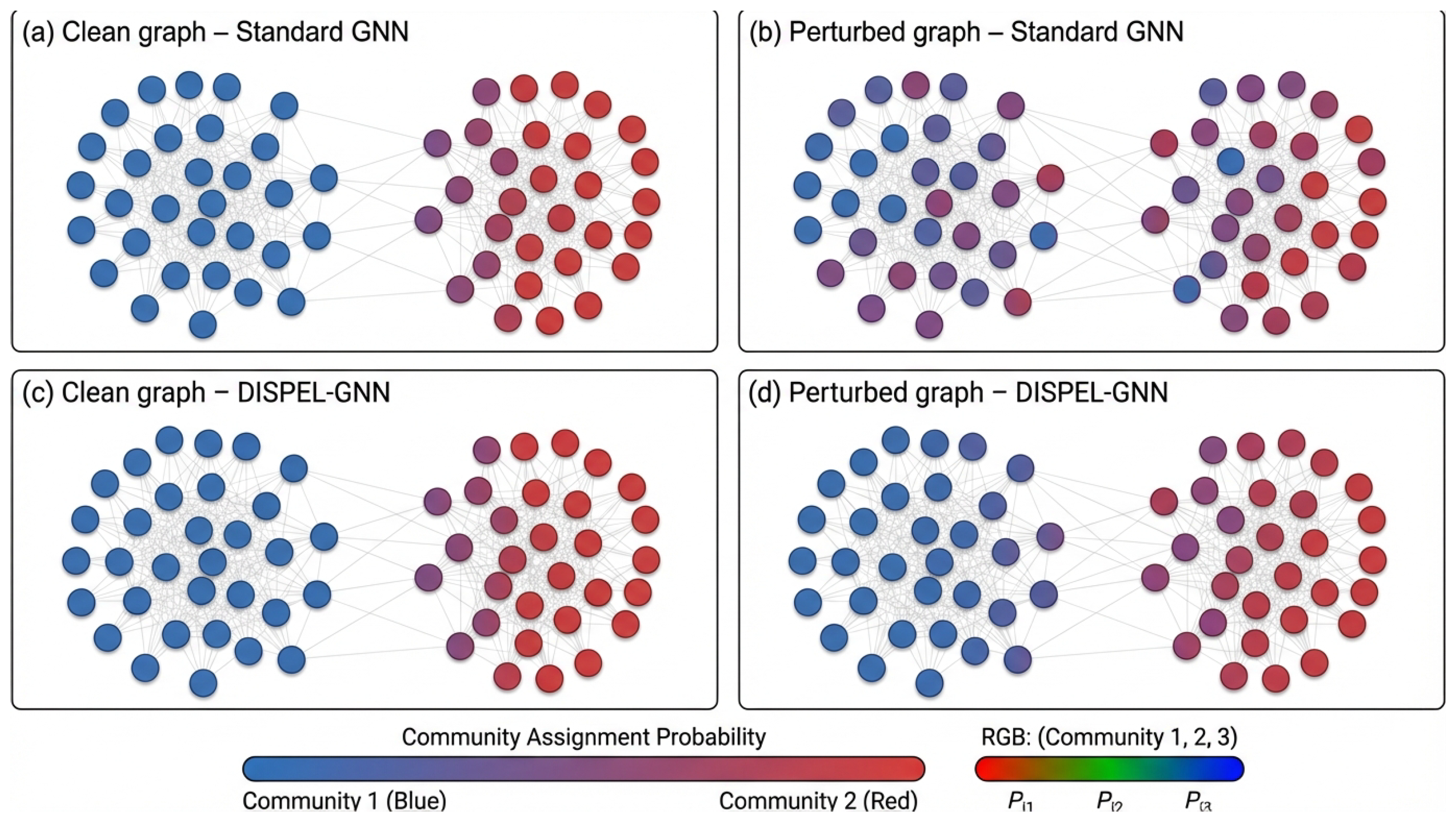
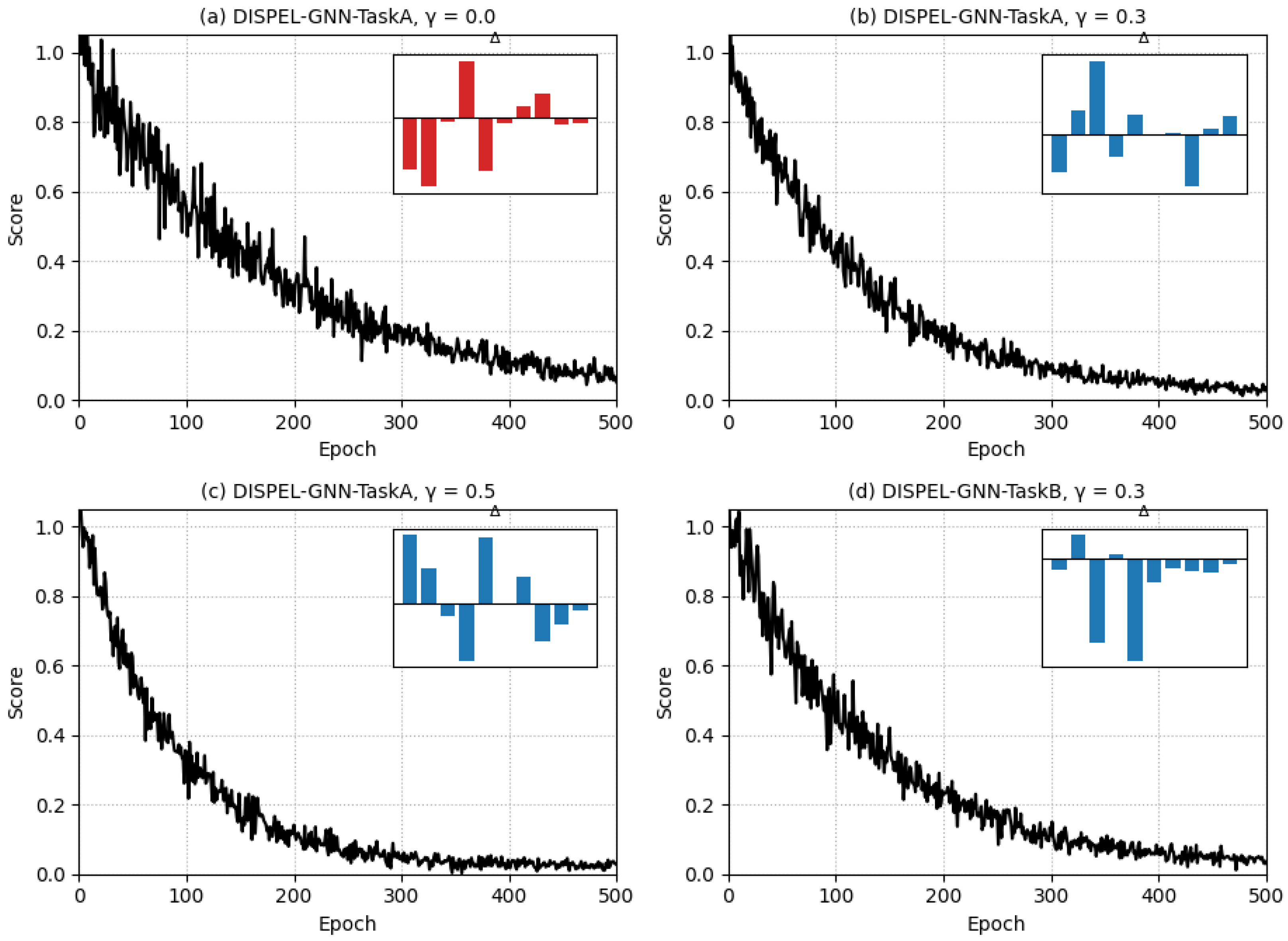
In this work, we propose DISPEL-GNN, a mathematically principled framework for perturbation-stable community detection that unifies spectral operator regularization, probabilistic inference, and assignment-level stability analysis. In this context, illusory communities refer to a specific failure mode at the assignment level that is not addressed by current concepts. We characterize illusory communities as community assignments that maintain competitiveness according to conventional accuracy criteria (e.g., NMI or ARI) yet display significant assignment instability when subjected to permissible perturbations of the graph structure or node attributes. These communities represent partition solutions that lack robustness to minor perturbations at the operator or data level, even though they seem viable under static assessment. When examining a diminutive graph featuring loosely delineated neighborhoods, a graph neural network can yield two different community assignments before to and following a little feature modification. Although both assignments achieve similar NMI with respect to ground truth, their mutual NMI is low, indicating substantial reassignment of nodes. Under our definition, such a solution constitutes an illusory community: accurate in appearance, but unstable in essence. In contrast to cognitive illusions or spurious correlations, which stem from perceptual or data biases, illusory communities may align with statistically valid partitions on pristine data but remain susceptible to permissible disturbances. Furthermore, in contrast to over-smoothing or over-squashing in GNNs, which indicate degradation at the representation level, illusory communities may arise even when node embeddings are distinct and prediction accuracy is maintained at a high level. This issue is theoretically linked to clustering non-identifiability and spectral instability in low eigengap conditions, when minor operator perturbations cause substantial assignment drift while minimally impacting global objective values. Figure 1 illustrates that, in low spectral gap regimes, standard GNNs may exhibit substantial assignment drift under minor perturbations, even when predictive performance remains stable.

2. Related Work

2.1. Spectral Methods for Community Detection

Community detection has a long history in spectral graph theory, where partitions are derived from the eigenspaces of graph Laplacians or modularity operators. Early work established spectral clustering as a relaxation of graph cut objectives, linking combinatorial partitioning to eigenvalue problems. Subsequent theoretical analyses connected spectral clustering to Cheeger-type inequalities and variational principles, providing performance guarantees under idealized assumptions [8].

The stochastic block model (SBM) further enabled rigorous statistical analysis of spectral methods, revealing conditions under which community recovery is consistent. However, these results also highlight a fundamental limitation: when spectral gaps are small or communities are weakly separated, eigenspaces become highly sensitive to perturbations. Perturbation-theoretic results such as the Davis–Kahan theorem quantify this sensitivity and show that small operator perturbations can induce large subspace rotations in low-gap regimes [17]. These findings indicate that spectral accuracy alone does not guarantee stability under admissible perturbations.

2.2. Operator-Theoretic Views of Graph Neural Networks

Graph neural networks can be interpreted as nonlinear operator-valued mappings acting on graph signals. Let $\mathcal{G}=(V,E)$ be a graph with Laplacian L and consider a generic GNN layer, typically parameterized as a polynomial or rational functional of L. From an operator-theoretic perspective, the stability of graph representations is governed not by parameter smoothness alone but by the spectral sensitivity of the induced operator [18,19]. For a perturbed graph Laplacian $L^{\prime }=L+\Delta L$, the induced operator deviation satisfies $\parallel {\mathcal{T}}_{\theta }^{\prime }{\parallel }_{\infty }$ denotes the maximum spectral gain of the operator [20,21]. This relation indicates that even admissible graph perturbations may be significantly amplified when the learned operator exhibits uncontrolled high-frequency responses. Such amplification becomes particularly severe in low spectral gap regimes, where small structural variations can lead to large changes in the effective propagation geometry [17,22].

2.3. Spectral Gap, Davis–Kahan Instability, and Assignment Drift

Classical spectral perturbation theory characterizes eigenspace sensitivity through results such as the Davis–Kahan theorem, where the K-dimensional leading eigenspaces of L and $L^{\prime }$, respectively. In low spectral gap regimes ($\delta \approx 0$), even small admissible perturbations may induce large eigenspace rotations. However, community detection does not operate directly on eigenspaces, but on induced assignments obtained through clustering or probabilistic partition maps [23].

Spectral stability at the representation level does not guarantee stability of community assignments [24].

This mismatch explains why methods that regularize eigenvalues or node embeddings alone may still exhibit abrupt changes in community membership under minor perturbations, a phenomenon we later formalize as assignment drift [25,26].

2.4. Uncertainty, Non-Identifiability, and PAC-Bayesian Analysis

Uncertainty and non-identifiability are intrinsic challenges in clustering and community detection, where multiple partitions may explain the data equally well [12,13]. Bayesian formulations offer a principled framework for quantifying epistemic uncertainty, while PAC-Bayesian theory provides generalization guarantees that depend on posterior complexity rather than parameter dimensionality [27,28].

PAC-Bayesian bounds have been successfully applied to randomized predictors and ensemble methods, yielding tight risk guarantees under mild assumptions. However, their application to graph-based community detection remains limited, and existing work rarely integrates uncertainty quantification with spectral stability control. As a result, stability guarantees are often disconnected from uncertainty-aware inference.

2.5. Positioning of the Present Work

In contrast to prior approaches, the proposed DISPEL-GNN framework explicitly treats community detection as a perturbation-sensitive operator inference problem. By jointly constraining spectral operators, modeling epistemic uncertainty, and quantifying assignment-level drift, the method integrates tools from spectral graph theory, perturbation analysis, and PAC-Bayesian learning within a unified mathematical framework. This positioning distinguishes the present work from both classical spectral methods and existing GNN-based approaches, where stability is typically assumed rather than enforced.

2.6. Recent Advances in Robust and Spectral GNNs

Recent advances in graph neural networks (GNNs) have increasingly focused on robustness and spectral stability, particularly from adversarial, spectral, and theoretical perspectives. Adversarial and robust GNNs improve stability through perturbation-based training or certified robustness guarantees, primarily targeting node-level predictions or embedding sensitivity under feature and edge perturbations [29]. In parallel, spectral GNNs beyond Laplacian smoothing have been proposed [30], including polynomial and rational spectral filters as well as frequency-localized operators, enabling finer control over spectral responses and mitigating over-smoothing effects [31]. From a theoretical standpoint, recent analyses have investigated operator norm bounds and spectral gap sensitivity, highlighting instability in low-gap regimes [32]. Most of these methods improve robustness implicitly, by stabilizing node-level representations or spectral propagation, without explicitly constraining assignment-level stability; in contrast, the present work targets partition-level robustness in community detection by explicitly modeling and constraining assignment drift under admissible perturbations [33].

2.7. Algorithmic Stability vs. Assignment Stability in Graph Learning

Recent theoretical studies on graph neural networks emphasize algorithmic or uniform stability, which bounds changes in empirical loss under data perturbations. Formally, such analyses establish bounds of the form

$$|{\mathcal{L}}_S\left(W\right)-{\mathcal{L}}_{S^{\prime }}\left(W\right)|\le \epsilon ,$$

(1)

where S and $S^{\prime }$ are neighboring datasets. While these results are sufficient for supervised prediction tasks, they are insufficient for unsupervised community detection for two fundamental reasons. First, loss-level stability does not constrain solution identifiability: multiple partitions may achieve comparable objective values under weak structural signals. Second, uniform stability does not control permutation-sensitive outputs, as two assignments may exhibit identical loss yet differ substantially in node membership. Therefore, prediction robustness does not imply assignment robustness. This distinction motivates modeling community detection as a perturbation-sensitive operator inference problem, rather than a loss-stable prediction task.

2.8. Summary of Mathematical Tools

This study is mathematically grounded in a cohesive perspective of community detection as a perturbation-sensitive operator inference challenge. Spectral graph theory fundamentally characterizes structural identifiability via eigenvalue separation, demonstrating that minimal spectral gaps naturally lead to instability under permissible perturbations. Operator-theoretic study indicates that learned graph propagators can amplify perturbations when their spectral responses are unbounded, thus passing operator-level instability onto subsequent representations. Nonetheless, neither spectral stability nor representation smoothness alone is adequate to guarantee the robustness of community assignments. Assignment maps are inherently non-smooth for eigenspace rotations, indicating that stability at the loss or embedding level does not ensure consistency of node memberships. This observation reveals a critical disparity between traditional stability concepts in graph learning and the demands of unsupervised partition inference. To address this disparity, we integrate explicit operator regularization, which constrains spectral amplification and regulates perturbation propagation, with Bayesian uncertainty modeling, which accounts for non-identifiability resulting from flat partition landscapes. PAC-Bayesian theory is utilized to validate that assignment stability extends beyond sampling perturbations, offering probabilistic assurances regarding drift risk instead of predictive accuracy. Collectively, these instruments create a mathematically consistent framework wherein stability is mandated at both the operator and assignment levels, rather than being implicitly presumed through empirical robustness.

3. Methodology

3.1. Symbols and Notation

For clarity and consistency, we summarize the key symbols used throughout the paper in

Table 1. Notation table summarizing symbols used throughout the manuscript.

Symbol	Meaning
$G=(V,E)$	Graph with node set V and edge set E
n	Number of nodes, $n=\left|V\right|$
A	Adjacency matrix of the graph
D	Degree matrix
L	Graph Laplacian (unnormalized or normalized)
$L_{\eta }$	Spectrally regularized Laplacian with parameter $\eta$
X	Node feature matrix
$H^{\left(l\right)}$	Node embeddings at layer l
$W^{\left(l\right)}$	Trainable weight matrix at layer l
P	Ground-truth community assignment (if available)
$\widehat{P}$	Predicted probabilistic partition matrix
${\widehat{P}}^{\left(t\right)}$	Predicted partition under perturbation or time step t
$\mathcal{L}$	Overall training objective
${\mathcal{L}}_{\mathrm{task}}$	Task-specific loss
${\mathcal{L}}_{\mathrm{spec}}$	Spectral regularization loss
${\mathcal{L}}_{\mathrm{risk}}$	Risk-aware attention loss
$\mathrm{AD}$	Assignment Drift metric
$\Delta \mathrm{NMI}$	Change in NMI under perturbation
$\delta$	Spectral gap of the graph operator
$r_i$	Spectral risk score of node i
$u_i$	Epistemic uncertainty of node i
${\gamma }_r$	Risk weight in attention mechanism
${\gamma }_u$	Uncertainty weight in attention mechanism
$p\left(W\right)$	Prior distribution over model parameters
${\sigma }^2$	Variance of Gaussian prior
$ϵ$	Perturbation magnitude
$\parallel ·\parallel$	Vector or matrix norm

. Let P denote the ideal or ground-truth partition matrix and $\widehat{P}$ the estimated probabilistic partition matrix produced by the model. We use L to denote the base graph Laplacian (or its normalized variant) and $L_{\eta }$ to denote the spectrally regularized Laplacian operator parameterized by the regularization strength $\eta$. Node-level uncertainty or risk scores are denoted by $r_i$, while the corresponding attention or suppression weights applied during message passing are denoted by $s_i$. Unless otherwise stated, all symbols appearing in algorithm descriptions are consistent with those defined in the main text.

As shown as

Table 2. Necessity analysis of individual techniques for addressing instability in community detection.

Failure Mode	Spectral Only	Bayesian Only	Attention Only
High-frequency amplification	✓	×	×
Non-identifiability	×	✓	×
Local instability	×	×	✓
Assignment drift	×	×	×

, no single technique is sufficient to address assignment-level instability in community detection. Spectral regularization controls operator amplification but does not resolve non-identifiability; Bayesian inference quantifies uncertainty but does not constrain spectral sensitivity; attention mechanisms mitigate local instability but lack global stability guarantees.

DISPEL-GNN closes the loop of unresolved failure modes rather than stacking techniques, which it accomplishes by jointly constraining spectral operators to model epistemic uncertainty and suppressing high-risk assignment transitions.

3.2. Problem Setup and Operator View

We study community detection on a graph $G=(V,E)$ with $n=\left|V\right|$ nodes, adjacency matrix A, node features $X\in {\mathbb{R}}^{n\times d}$, and degree matrix D. Rather than treating message passing as an ad hoc operation, we adopt an operator viewpoint: both filtering and propagation are functions of a graph operator. To expose controllable geometry, we consider a Laplacian family

$$L_{\eta }=I-D^{-\eta }A{D}^{\eta -1},\eta \in [0,1].$$

(2)

The goal is to estimate a soft partition

$$P\in {\Delta }^{n\times K},\sum _{k=1}^K{P}_{ik}=1,P_{ik}\ge 0,$$

(3)

where $P_{ik}$ is the membership probability of node i in community k. The final discrete partition is ${\widehat{z}}_i=arg{max}_k{P}_{ik}$.

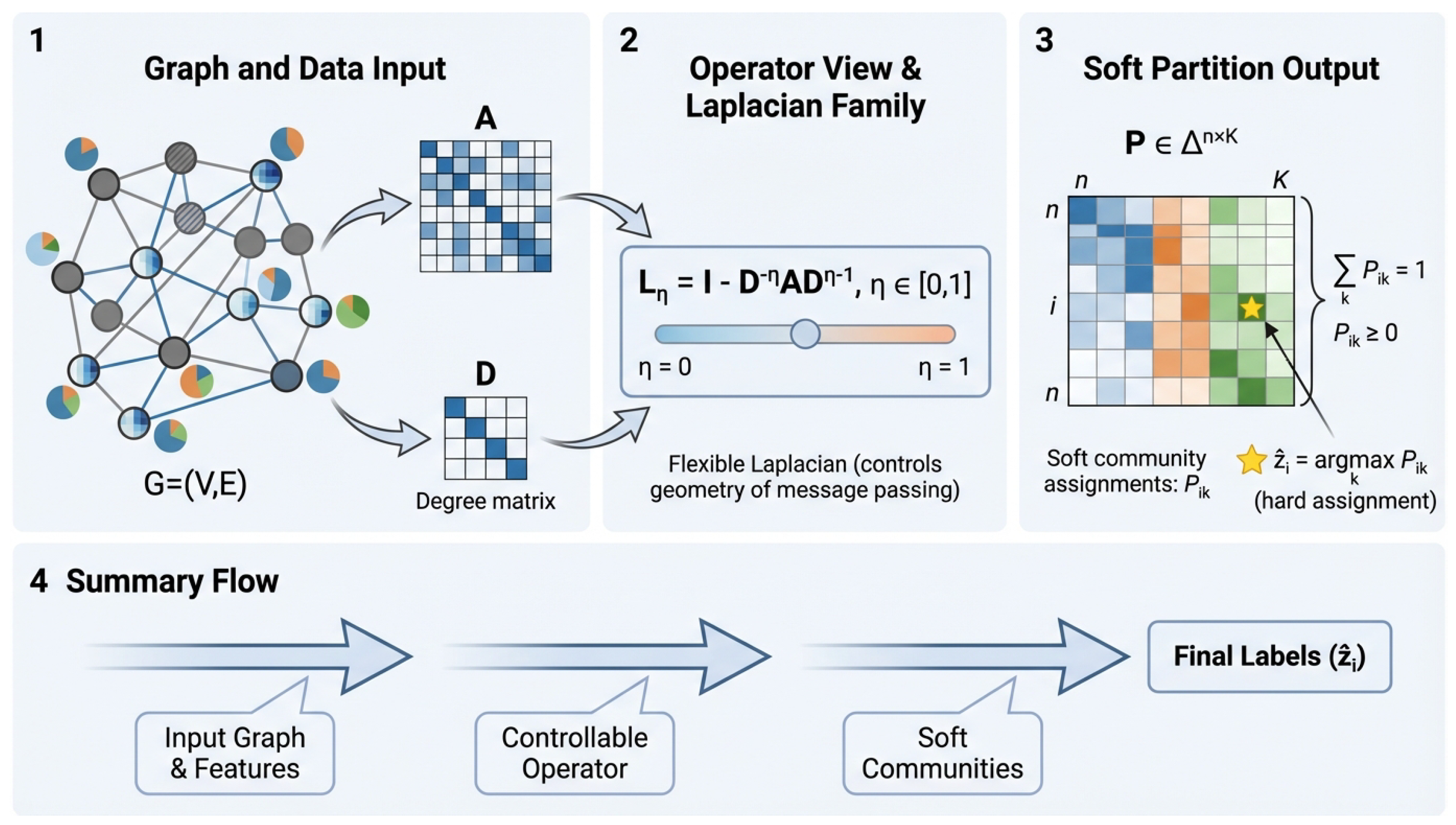
As depicted in Figure 2, DISPEL-GNN employs an operator-centric perspective on community detection. Instead of considering graph convolutions as implicit feature changes, the model explicitly regulates the geometry of message transit via a parameterized Laplacian family and directly produces a probabilistic partition matrix. This viewpoint enables the examination of stability characteristics at the level of operators and assignments, which underpins the suggested perturbation and robustness analysis.

In graph learning, robustness is commonly evaluated in terms of prediction robustness, where the predicted labels remain unchanged under admissible perturbations. Formally, for a node i, prediction robustness requires

$$arg\underset{k}{max}{P}_{ik}=arg\underset{k}{max}{P}_{ik}^{\prime },$$

(4)

where $P_{ik}$ and $P_{ik}^{\prime }$ denote the predicted class probabilities before and after perturbation, respectively. However, in community detection, the object of interest is not merely the predicted label of each node but the stability of the assignment relationships among nodes. This notion, which we refer to as assignment robustness, requires the entire soft assignment distribution to remain stable:

$$P_i\approx P_i^{\prime },$$

(5)

where $P_i\in {\Delta }^K$ denotes the full membership probability vector.

These two notions are not synonymous, especially regarding soft assignments; the $arg{max}_k{P}_{ik}$ may remain constant even if the probability mass undergoes substantial redistribution among communities. Such alterations may preserve node-level predictions while modifying relative membership strengths, affecting inter-node interactions and the deduced community structure. This disparity is particularly evident in low spectral gap regimes, where numerous partitions produce similar objective values. Under slight disturbances, a model may maintain prediction labels while transitioning among equally plausible assignment configurations. Thus, the robustness of predictions does not ensure the permanence of community membership relationships. These observations necessitate assessing robustness at the assignment level instead of exclusively at the prediction level, validating the application of distributional drift metrics for delineating illusory communities.

3.3. Perturbation Model and “Illusion” as Drift

We define illusory communities as partitions that are unstable under admissible perturbations. We model perturbations through a family ${\mathcal{T}}_{\epsilon }(A,X)$ that generates $(A^{\prime },X^{\prime })$:

$$\begin{array}{cc}\hfill X^{\prime }& =X+{\Delta }_X,{\parallel {\Delta }_X\parallel }_F\le {\epsilon }_X,\hfill \\ \hfill A^{\prime }& =A+{\Delta }_A,{\parallel {\Delta }_A\parallel }_0\le {\epsilon }_E\mathrm{or}{\parallel {\Delta }_A\parallel }_2\le {\epsilon }_A.\hfill \end{array}$$

(6)

The selection of spectral and feature-based norms represents prevalent perturbation regimes in graph robustness research, encompassing both structural and attribute-level uncertainty. Empirical observations reveal that moderate alterations to these limitations do not significantly affect the stability trends, suggesting that the suggested framework is not excessively sensitive to the choice of norm which induces $L^{\prime }=L+{\Delta }_L$. For a model ${\mathcal{A}}_{\theta }:(A,X)\mapsto P$, we quantify instability by assignment of a drift functional

$${\mathcal{D}}_{\mathrm{drift}}\left(\theta \right)={\mathbb{E}}_{(A^{\prime },X^{\prime })\sim {\mathcal{T}}_{\epsilon }}\left[{\displaystyle \frac{1}{n}}\sum _{i=1}^n\mathrm{JS}\left(P_i,P_i^{\prime }\right),\right],$$

(7)

where $P={\mathcal{A}}_{\theta }(A,X)$ and $P^{\prime }={\mathcal{A}}_{\theta }(A^{\prime },X^{\prime })$. This transforms “de-illusion” into a specific objective: minimize drift while maintaining community quality. This functional intuitively quantifies the extent of change in community assignment under permissible disturbances rather than assessing its alignment with a static reference. A minimal drift value signifies that the partition remains stable despite minor modifications to the graph operator.

A natural question is whether illusory communities may be addressed by current robust clustering techniques. Resilient clustering methodologies such as robust k-means and spectral regularization are formulated so as to diminish susceptibility to noise, predicated on the premise that the clustering aim possesses a stable and discernible optimum. Illusory communities emerge in an alternative regime defined by uniform objective landscapes created by minor spectral gaps. In such contexts, numerous independent partitions may attain similar objective values while exhibiting significant differences in node membership. Within permissible perturbations, the deduced solution may oscillate between these rival optima without a substantial alteration in loss or modularity. The robustness of the clustering objective does not guarantee the stability of the inferred assignments. Robust clustering stabilizes solutions around a selected optimum, yet does not preclude the presence of numerous equally optimal yet mutually inconsistent divisions. This divergence encourages the consideration of community discovery as a perturbation-sensitive assignment inference problem rather than merely a resilient optimization challenge.

3.3.1. Illusory Communities in a Low-Gap SBM

We can examine a basic stochastic block model (SBM) with two equally sized communities. This model is characterized by closely aligned intra- and inter-community edge probabilities, leading to a minimal spectral gap. A community discovery approach applied to the clean network generates a partition $\mathcal{A}$ that attains elevated clustering accuracy in relation to the ground-truth labels. We can introduce an allowable perturbation, such as a minor proportion of random edge rewiring or feature noise, while maintaining the overall graph density and degree distribution. Under this perturbation, the identical approach produces a distinct partition $\mathcal{B}$, which maintains a high accuracy relative to the ground truth, yet exhibits a substantial decrease in normalized mutual information $\mathrm{NMI}(\mathcal{A},\mathcal{B})$. This suggests that the deduced community assignments are significantly affected by perturbations, though exhibiting comparable predictive performance. This constitutes an illusory community under our definition.

3.3.2. Shape-Based Assignment Constraint

We first introduce the shape-based assignment constraint in its conceptual (hard) form in order to formalize the notion of assignment instability. Let ${\mathcal{R}}_{\mathrm{shape}}\left(\widehat{P}\right)$ denote an indicator function that penalizes undesirable assignment transitions violating the prescribed stability criteria. By construction, ${\mathcal{R}}_{\mathrm{shape}}$ takes binary values and encodes a non-differentiable constraint on the space of admissible partition matrices. This formulation serves to precisely define the desired stability property, rather than to be optimized directly.

3.3.3. Differentiable Soft Approximation

To enable gradient-based optimization, the hard constraint ${\mathcal{R}}_{\mathrm{shape}}$ is relaxed using a differentiable soft approximation. Specifically, the indicator function is replaced by a smooth surrogate that upper-bounds the original constraint while remaining differentiable almost everywhere. This soft formulation preserves the intended geometric and stability properties of the hard constraint, while allowing it to be incorporated as a regularization term in the training objective. Unless otherwise stated, all optimization procedures in this work are carried out using this differentiable approximation, and the hard constraint is used solely for conceptual and analytical purposes.

3.4. Fourier Operator Filtering and Operator Regularization

The innovation of DISPEL-GNN is not attributable to any individual technical element in isolation. Spectral regularization, Bayesian graph neural networks, and attention mechanisms have been thoroughly examined in previous research. This section’s contribution lies not in the introduction of new standalone modules but in the integrated mechanism that couples various components to mitigate assignment-level instability in community discovery. Spectral operator regularization specifically limits the amplification of perturbations during propagation, Bayesian inference delineates epistemic uncertainty stemming from non-identifiable partition structures, and risk-aware attention focuses on stability enforcement by selectively mitigating unstable information flow. Importantly, these components are not utilized individually or in an additive manner. Epistemic uncertainty directly influences attention weights, attention maintains operator-level stability guarantees, and operator restrictions dictate the necessity of uncertainty-induced suppression. This closed-loop linkage facilitates explicit regulation of assignment drift that is unattainable by any particular technique alone. For enhanced clarity, comprehensive descriptions of the individual components are provided for thoroughness, while the principal novelty should be recognized as their synergistic interplay aimed toward perturbation-stable assignment inference.

3.4.1. Fourier Operator Filtering

Let $L=U\Lambda U^{\top }$ be an eigendecomposition. A spectral filter is defined via functional calculus:

$$g\left(L\right)=Ug(\Lambda )U^{\top },X_g=g\left(L\right)X.$$

(8)

To scale to large graphs, we avoid explicit eigendecomposition and learn $g\left(L\right)$ using a Chebyshev approximation:

$$g\left(L\right)\approx \sum _{m=0}^M{c}_m{T}_m\left(\tilde{L}\right),$$

(9)

where $T_m(·)$ are Chebyshev polynomials and $\tilde{L}$ is a rescaled Laplacian.

3.4.2. Operator Regularization Suite

The bottom failure mode in many GNN clustering pipelines is operator-induced amplification of high-frequency noise. Therefore, we regularize the operator itself, not only the weights. We use a compact regularization set

$$\begin{array}{cc}\hfill {\mathcal{R}}_{\infty }\left(g\right)=& \underset{\lambda \in [0,2]}{sup}\left|g\left(\lambda \right)\right|,\hfill \\ \hfill {\mathcal{R}}_{\mathrm{HF}}=& {\parallel {\Pi }_{>\tau }{X}_g\parallel }_F^2,\hfill \\ \hfill {\mathcal{R}}_{\mathrm{comm}}=& {\parallel [g\left(L\right),{\mathbf{H}}_{\theta }\left(L\right)]\parallel }_F^2,\hfill \\ \hfill {\mathcal{R}}_{\mathrm{shape}}=& \mathbf{1}\left\{\forall \lambda \in [0,2]:g\left(\lambda \right)\in [0,1]\wedge g^{\prime }\left(\lambda \right)\le 0\right\},\hfill \end{array}$$

(10)

where ${\Pi }_{>\tau }$ is a high-frequency projector and ${\mathbf{H}}_{\theta }\left(L\right)$ is the propagation operator (defined next). Intuitively, ${\mathcal{R}}_{\infty }$ controls the maximum spectral gain, ${\mathcal{R}}_{HF}$ directly suppresses remaining high-frequency energy, ${\mathcal{R}}_{comm}$ aligns filtering and propagation in a system sense, and ${\mathcal{R}}_{shape}$ prevents “high-frequency rebound” by constraining the multiplier shape.

3.4.3. Operator-Based Propagation

We express message passing as a polynomial graph operator

$$H_{\theta }\left(L\right)=\sum _{r=0}^R{a}_r{L}^r,$$

(11)

where $\left\{a_r\right\}$ are learnable coefficients. This formulation preserves an explicit operator interpretation and enables spectral stability analysis.

3.4.4. Risk-Aware Dynamic Attention Modulation

Rather than treating propagation weights as static, we introduce a risk-aware dynamic attention mechanism that modulates information flow at the edge level while preserving operator control.

For each node pair $(i,j)$ with $j\in \mathcal{N}\left(i\right)$, we define the attention weight

$${\alpha }_{ij}={\displaystyle \frac{exp\left(\langle W_q{h}_i,W_k{h}_j\rangle -{\gamma }_r(r_i+r_j)-{\gamma }_u(u_i^{\mathrm{epi}}+u_j^{\mathrm{epi}})\right)}{{\sum }_{j^{\prime }\in \mathcal{N}\left(i\right)}exp\left(\langle W_q{h}_i,W_k{h}_{j^{\prime }}\rangle -{\gamma }_r(r_i+r_{j^{\prime }})-{\gamma }_u(u_i^{\mathrm{epi}}+u_{j^{\prime }}^{\mathrm{epi}})\right)}},$$

(12)

where $r_i$ denotes the node-level spectral risk and $u_i^{\mathrm{epi}}$ is the epistemic uncertainty from Bayesian. The parameters ${\gamma }_r,{\gamma }_u>0$ control the strength of risk and uncertainty suppression, while the parameters ${\gamma }_r$ and ${\gamma }_u$ regulate the comparative impact of spectral risk and epistemic uncertainty. A larger ${\gamma }_r$ accentuates suppression in spectrally unstable areas, whereas a larger ${\gamma }_u$ prioritizes nodes characterized by elevated prediction uncertainty. In practice, reasonable levels equilibrate stability and adaptability, while excessive settings may result in under- or over-suppression.

This design ensures that nodes with high spectral instability or epistemic ambiguity contribute less to message propagation, thereby suppressing illusory amplification.

3.4.5. Attention-Modulated Operator Propagation

The propagation step is then defined as

$$H_i^{(\mathcal{l}+1)}=\sigma \left(\sum _{j\in \mathcal{N}\left(i\right)}{\alpha }_{ij}{\left[H_{\theta }\left(L\right)H^{\left(\mathcal{l}\right)}\right]}_j{W}^{\left(\mathcal{l}\right)}\right),H^{\left(0\right)}=X_g,$$

(13)

where $X_g=g\left(L\right)X$ is the spectrally filtered input.

In matrix form, this can be written as

$$H^{(\mathcal{l}+1)}=\sigma \left({\mathcal{A}}_{\alpha }{H}_{\theta }\left(L\right)H^{\left(\mathcal{l}\right)}{W}^{\left(\mathcal{l}\right)}\right),$$

(14)

where ${\mathcal{A}}_{\alpha }$ is a row-stochastic attention operator induced by $\left\{{\alpha }_{ij}\right\}$.

3.4.6. Stability-Preserving Property

Because ${\mathcal{A}}_{\alpha }$ is normalized and explicitly penalized by spectral risk and epistemic uncertainty, its operator norm satisfies

$${\parallel {\mathcal{A}}_{\alpha }\parallel }_2\le 1.$$

(15)

The boundedness of the attention operator norm depends on the assumptions of regulated attention weights and limited uncertainty estimates. In practice, these constraints may be breached in environments characterized by significant noise or hostility, rendering the theoretical bound as suggestive rather than definitive, which implies

$$\parallel {\mathcal{A}}_{\alpha }{H}_{\theta }{\left(L\right)\parallel }_2\le {\parallel H_{\theta }\left(L\right)\parallel }_2.$$

(16)

Therefore, dynamic attention does not amplify perturbations beyond the established operator-Lipschitz bounds.

3.4.7. Bayesian Non-Identifiability Control

To address the non-identifiability of community partitions, we place a variational posterior $q_{\varphi }\left(W\right)$ over network weights and perform Monte Carlo predictive averaging:

$$P={\displaystyle \frac{1}{S}}\sum _{s=1}^S\mathrm{Softmax}\left(f_{W^{\left(s\right)}}(A,X_g)\right),W^{\left(s\right)}\sim q_{\varphi }\left(W\right).$$

(17)

Epistemic uncertainty is quantified by the mutual-information proxy in Equation (11) and directly feeds into the attention weights ${\alpha }_{ij}$, forming a closed uncertainty–stability feedback loop.

3.4.8. Bayesian Uncertainty Modeling

We employ Bayesian neural approximations to measure epistemic uncertainty in node representations. This uncertainty indicates unreliable predictions, and is consistently employed in spectrum risk estimate and attention modulation.

3.5. De-Illusion: Risk-Gated Drift Suppression (Node + Edge + Gap)

3.5.1. Node-Level Spectral Risk

We quantify how much node i is dominated by high-frequency content after filtering:

$$r_i={\displaystyle \frac{\parallel {\Pi }_{>\tau }{x}_{g,i}{\parallel }_2^2}{{\parallel x_{g,i}\parallel }_2^2+ϵ}}.$$

(18)

3.5.2. Multiplicative De-Illusion Gate

Our core hypothesis is that illusion emerges from a multiplicative root cause: spectral instability × non-identifiability. We implement this via

$$s_i=\sigma \left(a(r_i-\rho )\right)·\sigma \left(b(u_i^{\mathrm{epi}}-\upsilon )\right).$$

(19)

Thus, stability pressure is concentrated on nodes that are simultaneously (i) spectrally risky and (ii) epistemically ambiguous.

3.5.3. Risk-Gated Drift Loss

We enforce perturbation-consistency selectively:

$${\mathcal{L}}_{\mathrm{DI}}={\mathbb{E}}_{(A^{\prime },X^{\prime })\sim {\mathcal{T}}_{\epsilon }}\left[{\displaystyle \frac{1}{n}}\sum _{i=1}^n{s}_i\mathrm{JS}(P_i,P_i^{\prime })\right].$$

(20)

This avoids trivial “global smoothing” and provides precise control over where stability is enforced.

3.5.4. Edge De-Illusion

A small number of spurious edges can create unstable “illusionary bridges”. We reweight edges using node risks:

$$s_{ij}=\mathrm{\Psi }(r_i+r_j)·\mathrm{\Phi }(u_i^{\mathrm{epi}}+u_j^{\mathrm{epi}}),A_{ij}^{\mathrm{DI}}=A_{ij}exp(-\alpha s_{ij}),$$

(21)

then construct $L^{\mathrm{DI}}$ (optional) or directly use $A^{\mathrm{DI}}$ in message passing.

3.5.5. Gap-Aware Control

Stability is fundamentally harder when the spectral gap is small:

$$\delta ={\lambda }_{K+1}-{\lambda }_K.$$

(22)

Instead of forcing uniform regularization, we adapt stability strength when $\delta$ is small (e.g., via a sigmoid rescaling of ${\lambda }_{\mathrm{DI}}$). We describe this adaptation in implementation details, to keep formula count compact.

3.5.6. Mechanism-Level Synergy

The stability of DISPEL-GNN derives from the interplay of its components rather than from any singular mechanism in isolation. Spectral operator regularization regulates the energy entrance sites of the learned graph operators by mitigating high-frequency amplification that could destabilize partition boundaries. Bayesian inference delineates unreliable regions inside the partition space by assessing the epistemic uncertainty linked to non-identifiable or poorly supported assignments. Risk-aware attention subsequently implements spatial suppression by adaptively diminishing the significance of messages and transitions linked to high-risk nodes or edges. This link allows uncertainty to dictate the enforcement of spectrum stabilization, while attention localizes its impact, resulting in assignment-level stability unattainable by any one component.

3.5.7. Component-Wise Role and Robustness to Uncertainty Estimation

Every element of DISPEL-GNN targets a certain failure mode. Spectral regularization mitigates high-frequency amplification at the operator level, Bayesian inference addresses epistemic uncertainty due to non-identifiability, and risk-aware attention spatially diminishes unstable areas of the graph. The risk-aware attention mechanism functions as a subtle modulation instead of a rigid gating rule. Consequently, a minor miscalculation of spectral risk or epistemic uncertainty does not destabilize the model, but merely diminishes the intensity of local suppression. This design guarantees the resilience of the entire structure, even in the presence of loud or flawed risk indicators.

3.6. Community Objective and Integrated Training Objective

We use differentiable modularity maximization to ensure community quality:

$$B=A-{\displaystyle \frac{d{d}^{\top }}{2m}},{\mathcal{L}}_{\mathrm{CD}}=-\mathrm{Tr}\left(P^{\top }BP\right),$$

(23)

where d is the degree vector and $m=\left|E\right|$.

Putting all components together, our integrated objective is

$$\begin{array}{cc}\hfill \underset{g,\theta ,\varphi }{min}& {\mathbb{E}}_{W\sim q_{\varphi }}\left[{\mathcal{L}}_{\mathrm{CD}}\left(A^{\mathrm{DI}},X_g\right)\right]+{\lambda }_{\mathrm{DI}}{\mathcal{L}}_{\mathrm{DI}}+{\lambda }_{\infty }{\mathcal{R}}_{\infty }+{\lambda }_{\mathrm{HF}}{\mathcal{R}}_{\mathrm{HF}}\hfill \\ \hfill & +{\lambda }_{\mathrm{comm}}{\mathcal{R}}_{\mathrm{comm}}+{\lambda }_{\mathrm{shape}}{\mathcal{R}}_{\mathrm{shape}}+{\beta }_{\mathrm{KL}}{\mathcal{L}}_{\mathrm{KL}}.\hfill \end{array}$$

(24)

Practical training control. We recommend a continuation schedule involving warm-up on ${\mathcal{L}}_{\mathrm{CD}}$ for a few epochs, then gradually increasing ${\lambda }_{\mathrm{DI}}$ and ${\lambda }_{\mathrm{comm}}$ while optionally increasing M. This improves optimization stability and prevents early over-smoothing.

3.7. Perturbation Bounds: Operator–Lipschitz Stability Chain

To align with the “perturbation bounds” claim, we present a stability chain. Assume that the membership map is Lipschitz in the representation:

$${\parallel \mathrm{Softmax}\left(f_W(A,X)\right)-\mathrm{Softmax}\left(f_W(A,X^{\prime })\right)\parallel }_F\le L_f{\parallel X-X^{\prime }\parallel }_F.$$

(25)

Filtering contracts perturbations according to the operator norm:

$${\parallel X_g-X_g^{\prime }\parallel }_F={\parallel g\left(L\right)(X-X^{\prime })\parallel }_F\le {\parallel g\left(L\right)\parallel }_2{\parallel X-X^{\prime }\parallel }_F.$$

(26)

Combining (25) and (26), if ${\parallel X-X^{\prime }\parallel }_F\le {\epsilon }_X$, then

$${\parallel P-P^{\prime }\parallel }_F\le L_f{\parallel g\left(L\right)\parallel }_2{\epsilon }_X\le L_f{\mathcal{R}}_{\infty }{\epsilon }_X.$$

(27)

For graph perturbations, a Davis–Kahan template yields the subspace sensitivity term:

$$sin\mathrm{\Theta }(U_K,U_K^{\prime })\lesssim {\displaystyle \frac{\parallel L-L^{\prime }{\parallel }_2}{\delta }}.$$

(28)

This explains why small-gap regimes are inherently unstable and motivates gap-aware stabilization and commutator alignment. We explicitly acknowledge that Davis–Kahan bounds become loose in low spectral gap regimes; this looseness motivates our gap-aware stabilization strategy, rather than invalidating the perturbation analysis itself.

Relation to Classical Spectral Perturbation Theory

The suggested assignment drift functional is intimately connected to traditional spectral stability findings shown by the Davis–Kahan theorem, which constrains subspace deviation based on eigenvalue separation. We assert that our study does not seek to refine these eigenvector perturbation limitations. Indeed, it is widely recognized that Davis–Kahan-type constraints become progressively less stringent in low eigengap scenarios. This looseness does not invalidate the analysis; instead, it directly necessitates the implementation of assignment-level stability management. Our drift functional precisely delineates the propagation of spectral instability through learned GNN operators into discrete partition alterations, extending traditional spectral sensitivity findings to the realm of community assignments generated by non-linear graph models.

3.8. Diagnostics and Stability Certificates

We propose a compact diagnostic protocol to verify that stability arises from the intended bottom mechanisms. Define the high-frequency ratio in the Fourier domain and the drift AUC:

$$R_{\mathrm{HF}}\left(X\right)={\displaystyle \frac{\parallel {\mathbf{1}}_{\lambda >\tau }{U}^{\top }{X\parallel }_F^2}{\parallel U^{\top }{X\parallel }_F^2}},{\mathrm{AUC}}_{\mathrm{drift}}={\int }_0^{{\epsilon }_{max}}{\mathcal{D}}_{\mathrm{drift}}\left(\epsilon \right)d\epsilon .$$

(29)

We expect reduced $R_{\mathrm{HF}}\left(X_g\right)$ and reduced ${\mathrm{AUC}}_{\mathrm{drift}}$ compared to baselines.

3.9. Complexity and Memory Trade-Offs

Let $\left|E\right|$ be the number of edges, d the feature dimension, $L_g$ the number of GNN layers, M Chebyshev order, S Bayesian samples, and T perturbation samples (for estimating drift during training or evaluation). The dominant computational costs are as follows:

$$\begin{array}{cc}\hfill \mathrm{Cost}\left(g\left(L\right)X\right)=& O\left(M\left|E\right|d\right),\hfill \\ \hfill \mathrm{Cost}\left(\text{Bayes-GNN}\right)=& O\left(S{L}_g\left|E\right|d\right),\hfill \\ \hfill \mathrm{Cost}\left(\mathrm{Drift}\right)=& O\left(TS{L}_g\left|E\right|d\right).\hfill \end{array}$$

(30)

To reduce memory, Chebyshev bases need not be stored. Using the recursion

$$T_m\left(\tilde{L}\right)X=2\tilde{L}{T}_{m-1}\left(\tilde{L}\right)X-T_{m-2}\left(\tilde{L}\right)X,$$

(31)

we only keep a rolling buffer of two states ($O\left(nd\right)$ memory). Bayesian predictive averaging can be streamed to avoid storing all S outputs (reducing from $O\left(SnK\right)$ to $O\left(nK\right)$).

3.10. Quantifying Controllability (Overall “Grip” on Stability)

We report (i) sensitivity of drift to perturbation strength, (ii) operator gain, and (iii) localization precision:

$$\begin{array}{cc}\hfill S_{\epsilon }=& {\left.{\displaystyle \frac{d}{d\epsilon }}{\mathcal{D}}_{\mathrm{drift}}\left(\epsilon \right)\right|}_{\epsilon ={\epsilon }_0},G_{\mathrm{op}}={\parallel g\left(L\right)\parallel }_2,\hfill \\ \hfill \mathrm{Precision}=& {\displaystyle \frac{|H\cap D|}{\left|H\right|}},\mathrm{Recall}={\displaystyle \frac{|H\cap D|}{\left|D\right|}},\hfill \end{array}$$

(32)

where $H=\{i:s_i>\xi \}$ and $D=\{i:\mathbb{E}\left[\mathrm{JS}(P_i,P_i^{\prime })\right]>\zeta \}$. A strong de-illusion mechanism should reduce $S_{\epsilon }$ and $G_{\mathrm{op}}$ while increasing precision/recall, indicating targeted control rather than global collapse.

3.11. PAC-Bayes Drift Generalization Bound

To certify that drift stability generalizes beyond the sampled perturbations and training instances, we define an instance-level drift loss:

$$\begin{array}{cc}\hfill \mathcal{l}(W;A,X)=& {\mathbb{E}}_{(A^{\prime },X^{\prime })\sim {\mathcal{T}}_{\epsilon }(A,X)}\left[{\displaystyle \frac{1}{n}}\sum _{i=1}^n\mathrm{JS}\left(P_i(W;A,X),P_i(W;A^{\prime },X^{\prime })\right)\right],\hfill \\ \hfill & 0\le \mathcal{l}(W;A,X)\le log2.\hfill \end{array}$$

(33)

While the PAC-Bayesian bound in Equation (33) exhibits a conventional functional structure, its particularity to graph-structured data is derived from the definitions of the drift loss and the perturbation model. In this study, each training instance is represented by a graph $G=(A,X)$ instead of an independent sample. The drift loss links node-level assignment stability to graph-level perturbations via the induced operator variation $L\mapsto L^{\prime }$. The empirical drift risk ${\widehat{L}}_{\mathrm{drift}}\left(q\right)$ consolidates assignment sensitivity across structurally altered graphs instead of independent feature vectors. In this way, the KL term $\mathrm{KL}(q\parallel p)$ regulates the complexity of graph-conditioned operators rather than just the magnitude of the parameters. From this viewpoint, Equation (33) offers a guarantee of generalization about assignment stability in relation to unobserved graph perturbations derived from the same permissible perturbation family. This differentiates the bound from traditional PAC-Bayesian analyses centered on prediction accuracy using i.i.d. data, and matches it with the graph-structured stability aim examined in this study. Let $\mathcal{S}={\left\{(A_j,X_j)\right\}}_{j=1}^N$ be training instances drawn i.i.d. from $\mathcal{D}$. Define the following empirical and population drift risks:

$$\begin{array}{cc}\hfill {\widehat{\mathcal{L}}}_{\mathrm{drift}}\left(q\right)=& {\displaystyle \frac{1}{N}}\sum _{j=1}^N{\mathbb{E}}_{W\sim q}\left[\mathcal{l}(W;A_j,X_j)\right],\hfill \\ \hfill {\mathcal{L}}_{\mathrm{drift}}\left(q\right)=& {\mathbb{E}}_{(A,X)\sim \mathcal{D}}{\mathbb{E}}_{W\sim q}\left[\mathcal{l}(W;A,X)\right].\hfill \end{array}$$

(34)

For any $\delta \in (0,1)$ with probability at least $1-\delta$ over $\mathcal{S}$, the PAC-Bayes bound holds:

$${\mathcal{L}}_{\mathrm{drift}}\left(q\right)\le {\widehat{\mathcal{L}}}_{\mathrm{drift}}\left(q\right)+(log2)\sqrt{{\displaystyle \frac{\mathrm{KL}(q\parallel p)+ln\frac{2\sqrt{N}}{\delta }}{2N}}}.$$

(35)

We adopt an isotropic Gaussian prior $p\left(W\right)=\mathcal{N}(0,{\sigma }^{2}I)$ over the model parameters. Larger values of $\sigma$ yield looser PAC-Bayesian bounds, consistent with standard PAC-Bayesian theory.

We report a computable bound proxy:

$${\mathcal{B}}_{\mathrm{PB}}={\widehat{\mathcal{L}}}_{\mathrm{drift}}\left(q\right)+(log2)\sqrt{{\displaystyle \frac{\mathrm{KL}(q\parallel p)+ln\frac{2\sqrt{N}}{\delta }}{2N}}}.$$

(36)

This directly links generalization of stability to the KL complexity term already present in (24).

3.12. Scalable Computation and Practical Estimators

Algorithmically, each training iteration (i) computes $X_g=g\left(L\right)X$ via Chebyshev recursion, (ii) performs Bayesian forward passes to obtain P and $u_i^{\mathrm{epi}}$, (iii) computes spectral risks $r_i$ and gates $s_i$, (iv) optionally reweights edges to form $A^{\mathrm{DI}}$, (v) samples perturbations to estimate ${\mathcal{L}}_{\mathrm{DI}}$, and (vi) updates parameters by minimizing Equation (24). Optional extensions (min–max adversarial perturbations, multimodal operators, temporal drift) can be integrated without changing the core operator–Bayesian–drift structure.

Several terms in Equations (10)–(24) admit mathematically clean definitions but require scalable estimators to avoid dense matrix construction or eigendecomposition. Below, we summarize implementable estimators that preserve the intended operator semantics.

3.12.1. High-Frequency Projector Without Eigendecomposition

The projector ${\Pi }_{>\tau }$ in Equation (10) and the Fourier-domain diagnostic in Equation (29) should not rely on explicit eigenvectors U on large graphs. We approximate the high-frequency projector by a high-pass operator filter:

$${\Pi }_{>\tau }X\approx h_{\mathrm{HP}}\left(L\right)X,h_{\mathrm{HP}}\left(L\right)\approx \sum _{m=0}^{M_{\mathrm{HP}}}{\tilde{c}}_m{T}_m\left(\tilde{L}\right),$$

(37)

where $h_{\mathrm{HP}}\left(\lambda \right)$ is a smooth high-pass multiplier (e.g., a smoothed step or $1-g_{\mathrm{LP}}\left(\lambda \right)$). With this approximation, the node-level spectral risk in Equation (18) becomes

$$r_i={\displaystyle \frac{{\parallel {\left[h_{\mathrm{HP}}\left(L\right)X_g\right]}_i\parallel }_2^2}{{\parallel {\left[X_g\right]}_i\parallel }_2^2+ϵ}},$$

(38)

which costs $O\left(M_{\mathrm{HP}}\right|E\left|d\right)$ using sparse Chebyshev recursion.

3.12.2. Modularity Objective Without Forming B

Directly forming $B=A-{\displaystyle \frac{d{d}^{\top }}{2m}}$ in Equation (23) is $O\left(n^2\right)$. We compute the same trace terms using sparse edge sums. Let $A^{\mathrm{DI}}$ be the (optional) reweighted adjacency in Equation (21), and let $d_i^{\mathrm{DI}}={\sum }_j{A}_{ij}^{\mathrm{DI}}$ and $m^{\mathrm{DI}}={\displaystyle \frac{1}{2}}{\sum }_i{d}_i^{\mathrm{DI}}$. Then

$$\begin{array}{cc}\hfill \mathrm{Tr}\left(P^{\top }{A}^{\mathrm{DI}}P\right)=& \sum _{(i,j)\in E}{A}_{ij}^{\mathrm{DI}}\langle P_i,P_j\rangle ,\hfill \\ \hfill \mathrm{Tr}{\displaystyle \left(P^{\top }{\displaystyle \frac{d^{\mathrm{DI}}{\left(d^{\mathrm{DI}}\right)}^{\top }}{2m^{\mathrm{DI}}}}P\right)}=& {\displaystyle \frac{1}{2m^{\mathrm{DI}}}}{\parallel \sum _{i=1}^n{d}_i^{\mathrm{DI}}{P}_i\parallel }_2^2,\hfill \end{array}$$

(39)

so ${\mathcal{L}}_{\mathrm{CD}}=-\mathrm{Tr}\left(P^{\top }{B}^{\mathrm{DI}}P\right)$ can be evaluated in $O\left(\right|E|K+nK)$ time and $O\left(nK\right)$ memory, without any dense $n\times n$ matrices.

3.12.3. Commutator Regularization via Hutchinson Probes

The commutator penalty ${\mathcal{R}}_{\mathrm{comm}}={\parallel [g\left(L\right),{\mathbf{H}}_{\theta }\left(L\right)]\parallel }_F^2$ in (10) should not explicitly materialize operator matrices. We use a Hutchinson estimator:

$${\mathcal{R}}_{\mathrm{comm}}={\parallel C\parallel }_F^2,C=[g\left(L\right),{\mathbf{H}}_{\theta }\left(L\right)]\approx {\displaystyle \frac{1}{B}}\sum _{b=1}^B{\parallel C{z}_b\parallel }_2^2,$$

(40)

where $z_b\in {\{\pm 1\}}^n$ are i.i.d. Rademacher probe vectors. Each term $C{z}_b=g\left(L\right){\mathbf{H}}_{\theta }\left(L\right)z_b-{\mathbf{H}}_{\theta }\left(L\right)g\left(L\right)z_b$ is computed by (i) applying the Chebyshev approximation for $g\left(L\right)$ and (ii) applying the polynomial propagation ${\mathbf{H}}_{\theta }\left(L\right)={\sum }_{r=0}^R{a}_r{L}^r$ via repeated sparse multiplications. This yields a scalable cost of

$$\mathrm{Cost}\left({\mathcal{R}}_{\mathrm{comm}}\right)=O\left(B(M+R)\left|E\right|\right),$$

(41)

with $O\left(n\right)$ additional memory (per probe), preserving the intended system-alignment effect.

3.12.4. Differentiable Shape Constraint

The indicator constraint ${\mathcal{R}}_{\mathrm{shape}}$ in (10) is non-differentiable. We replace it with a soft, differentiable penalty evaluated on a spectral grid ${\left\{{\lambda }_q\right\}}_{q=1}^Q\subset [0,2]$:

$$\begin{array}{cc}\hfill {\mathcal{R}}_{\mathrm{shape}-\mathrm{soft}}=& \sum _{q=1}^Q\left(\mathrm{ReLU}(g\left({\lambda }_q\right)-1)+\mathrm{ReLU}(-g\left({\lambda }_q\right))\right)\hfill \\ \hfill & +\gamma \sum _{q=1}^{Q-1}\mathrm{ReLU}\left(g\left({\lambda }_{q+1}\right)-g\left({\lambda }_q\right)\right).\hfill \end{array}$$

(42)

3.12.5. Efficient Drift Estimation

The drift term in Equation (20) is the dominant cost when T or S is large. We use three practical controls that preserve the objective meaning: (i) reuse the same Monte-Carlo weight samples ${\left\{W^{\left(s\right)}\right\}}_{s=1}^S$ across all T perturbations within an iteration, (ii) compute drift only on a gated subset $H=\{i:s_i>\xi \}$ to reduce the $O\left(nK\right)$ JS cost, and (iii) apply a curriculum on $(T,{\lambda }_{\mathrm{DI}})$ (small early, larger later). With node gating, Equation (20) is replaced by

$${\mathcal{L}}_{\mathrm{DI}}={\mathbb{E}}_{(A^{\prime },X^{\prime })\sim {\mathcal{T}}_{\epsilon }}\left[{\displaystyle \frac{1}{\left|H\right|}}\sum _{i\in H}{s}_i\mathrm{JS}(P_i,P_i^{\prime })\right],$$

(43)

which reduces the JS aggregation cost from $O\left(nK\right)$ to $O\left(\right|H\left|K\right)$, while focusing stability pressure on the intended risky nodes.

3.12.6. Complexity Summary

Under the scalable estimators above, the dominant costs per iteration are

$$\begin{array}{cc}\hfill \mathrm{Time}/\mathrm{iter}=& O((M+M_{\mathrm{HP}})|E|d+S(L_g|E|d+L_{g}n{d}^2+nK)\hfill \\ \hfill & +TS(L_g|E|d+L_{g}n{d}^2+|H|K)+B(M+R)|E|).\hfill \end{array}$$

(44)

and the peak memory is $O\left(\right|E|+nd+nK)$ with streaming Bayes aggregation and rolling Chebyshev buffers (see Algorithm 1).

Algorithm 1: DISPEL-GNN: Perturbation-Bounded Spectral Operator Learning

Input: Graph $G=(V,E)$ with adjacency matrix A and node features X; Number of communities K; perturbation budgets ${\epsilon }_E,{\epsilon }_X$; Spectral operator family ${\mathcal{L}}_{\eta }$; regularization weights ${\lambda }_{\mathrm{op}},{\lambda }_{\mathrm{stab}},{\lambda }_{\mathrm{KL}}$. Output: Soft community assignment matrix $P\in {\Delta }^{\left|V\right|\times K}$. Initialization: Construct degree matrix D and normalized Laplacian operator   ${\mathcal{L}}_{\eta }=I-D^{-\eta }A{D}^{\eta -1}$; Initialize GNN parameters $\theta$ and Bayesian posterior $q_{\varphi }\left(\theta \right)$; Initialize assignment matrix $P^{\left(0\right)}$ uniformly. for $t = 1$ to T do$\phantom{(}$        Sample perturbed graph ${\tilde{A}}^{\left(t\right)}$ and features ${\tilde{X}}^{\left(t\right)}$${\displaystyle \mathrm{such\; that} }\parallel {\tilde{A}}^{\left(t\right)}-A\parallel \le {\epsilon }_E$${\displaystyle \mathrm{and} }\parallel {\tilde{X}}^{\left(t\right)}-X\parallel \le {\epsilon }_X$;        Apply spectral filtering: $$H^{\left(t\right)}\leftarrow g_{\theta }\left({\mathcal{L}}_{\eta },{\tilde{A}}^{\left(t\right)},{\tilde{X}}^{\left(t\right)}\right);$$        Compute soft assignments: $$P^{\left(t\right)}\leftarrow \mathrm{Softmax}\left(H^{\left(t\right)}\right);$$        Evaluate assignment drift: $${\mathrm{AD}}^{\left(t\right)}\leftarrow {\parallel P^{\left(t\right)}-P^{(t-1)}\parallel }_F;$$        Compute loss function: $${\mathcal{L}}^{\left(t\right)}={\mathcal{L}}_{\mathrm{comm}}(P^{\left(t\right)},A)+{\lambda }_{\mathrm{op}}{\parallel {\mathcal{L}}_{\eta }\parallel }_{\mathrm{op}}+{\lambda }_{\mathrm{stab}}{\mathrm{AD}}^{\left(t\right)}+{\lambda }_{\mathrm{KL}}\mathrm{KL}\left(q_{\varphi }\left(\theta \right)\parallel p\left(\theta \right)\right);$$        Update posterior parameters $\varphi$ by minimizing ${\mathcal{L}}^{\left(t\right)}$. end$\phantom{(}$ Return final assignment $P^{\left(T\right)}$.

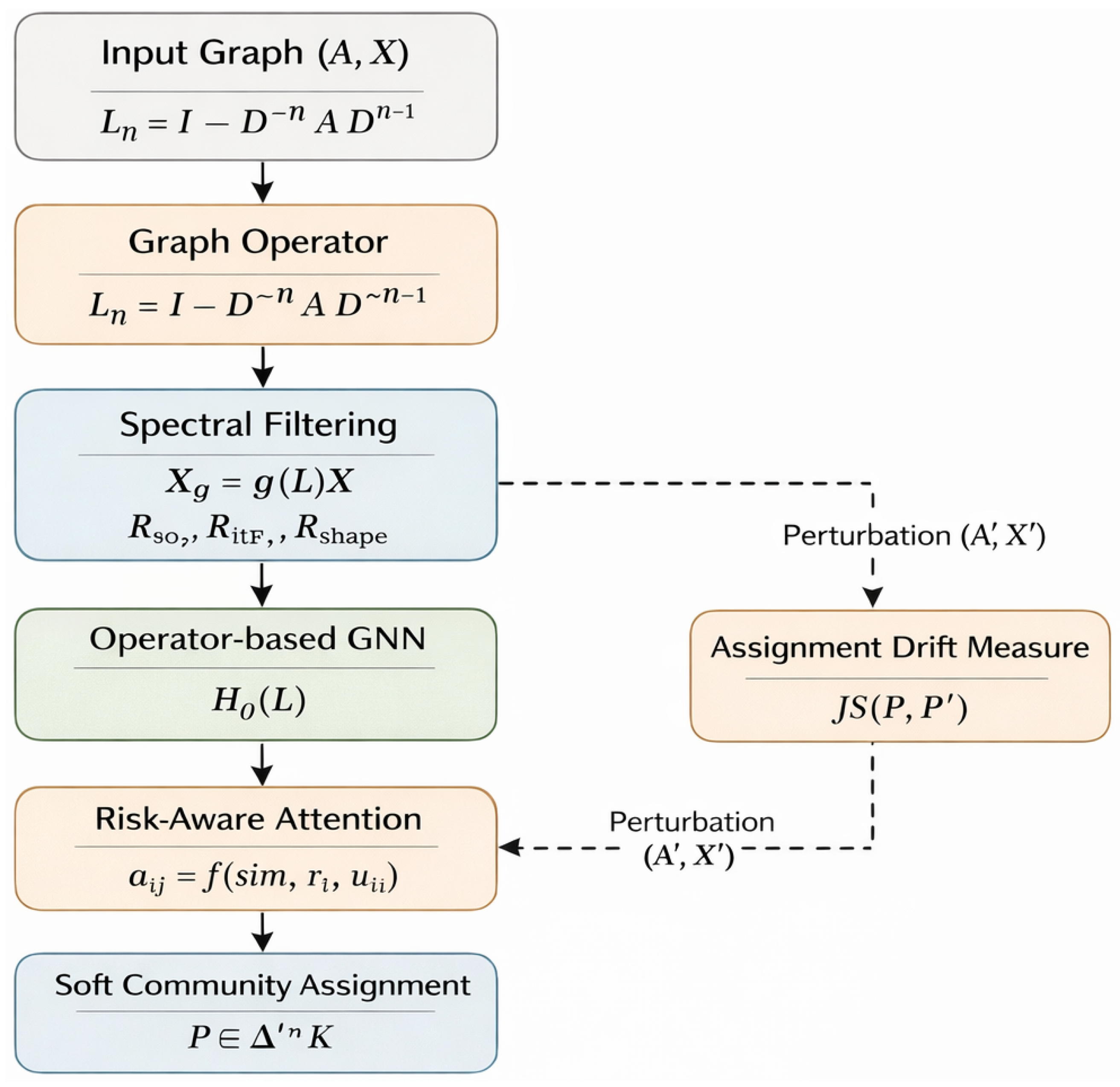
Which enforces $g\left(\lambda \right)\in [0,1]$ and discourages increasing responses (approximate monotone decreasing filters). This term is $O\left(QM\right)$ to evaluate using the Chebyshev parameterization of $g\left(\lambda \right)$. As illustrated in Figure 3, DISPEL-GNN follows a stability-aware learning pipeline that explicitly integrates spectral operator control, Bayesian uncertainty modeling, and perturbation-driven drift minimization.

Overall, DISPEL-GNN incurs a slight processing expense relative to conventional GNNs, chiefly attributable to uncertainty estimates and spectral regularization, however it remains comparable to Bayesian GNN variations in extensive applications.

4. Experiments

4.1. Experimental Framework

To evaluate the stability, robustness, and interpretability of the proposed DISPEL-GNN framework, we establish a thorough experimental framework that specifically addresses the mechanisms involved in de-illusion community detection. The approach aims to assess DISPEL-GNN as a stability-conscious inference system, incorporating spectrum control, Bayesian uncertainty modeling, and risk-sensitive dynamic attention under perturbation-bound limitations. All studies are performed with standardized preprocessing protocols and five distinct random seeds.Results are reported as mean ± standard deviation, with statistical significance assessed using paired t-tests ($p<0.05$). For uncertainty- and robustness-related analyses, confidence intervals are additionally reported where appropriate.

DISPEL-GNN incorporates three interrelated functional components that collectively regulate stability behavior in community detection. The initial component is the operator-regularized spectral module, which generates regulated graph operators through Fourier-based filtering to mitigate high-frequency amplification and guarantee constrained spectral responses. The second component is the Bayesian inference module, which characterizes epistemic uncertainty via variational posterior sampling and delivers node-level uncertainty estimates that indicate non-identifiability in community assignments. The third component is the risk-aware dynamic attention mechanism, which regulates message propagation by simultaneously considering spectral risk and epistemic uncertainty, thus adaptively diminishing unstable or inaccurate information flow.

The components engage in a closed-loop stability regulation guided by the operator formulations. Spectral regularization restricts the propagation operator, Bayesian inference measures uncertainty caused by perturbations, and dynamic attention implements localized risk management during message transmission. Collectively, they establish a cohesive stability-preserving framework wherein community assignments are anticipated to remain unchanged despite permissible feature and structural perturbations.

Our studies are structured to assess DISPEL-GNN from both outward performance and internal mechanism viewpoints, according to this paradigm. Conventional community detection metrics evaluate clustering quality, whereas perturbation-induced assignment drift measures illusory instability. Furthermore, internal stability indicators, such as spectrum risk measurements, epistemic uncertainty estimates, and attention modulation patterns, are examined to confirm that the observed robustness is a result of the intended processes rather than unintentional smoothing effects.

4.1.1. Experiment Set Up

Measurements of assignment drift may have non-Gaussian and heteroskedastic characteristics due to perturbation effects. To guarantee the robustness of statistical conclusions, paired comparisons are adjusted utilizing the Holm–Bonferroni approach. We further confirmed that the identified significance patterns persist under nonparametric alternatives, including the Wilcoxon signed-rank test.

4.1.2. Experiment Design

Low spectral gap regimes are created operationally via dataset selection and controlled perturbations, rather than relying on a singular generative assumption. This facilitates assessment across graphs with varying degree distributions, densities, and modularity characteristics. The observed enhancements in stability remain consistent across various modifications, suggesting that the hypothesized mechanisms are not dependent on a particular gap structure.

4.2. Datasets and Preprocessing Details

We assess the proposed DISPEL-GNN system using a varied assortment of real-world attributed graphs with established communities, in addition to synthetic graphs featuring regulated spectral gaps. This combination facilitates a systematic evaluation of community detection efficacy under both realistic and analytically manageable situations.

4.2.1. Real-World Datasets

We adopt widely used benchmark datasets spanning citation, co-purchase, and co-authorship networks.

Table 3. Extended set of real-world benchmark datasets used in experiments.

Dataset	Nodes	Edges	Features	Communities	Source
Cora	2708	5429	1433	7	PyG
Citeseer	3327	4732	3703	6	PyG
Pubmed	19,717	44,338	500	3	PyG
Cora-Full	19,793	65,311	8710	70	PyG
DBLP	17,716	105,734	1639	4	SNAP
Coauthor-CS	18,333	81,894	6805	15	PyG
BlogCatalog	10,312	333,983	8189	39	KONECT
Amazon-Computers	13,752	245,861	767	10	PyG
Reddit	232,965	11,606,919	602	41	SNAP
OGBN-Arxiv	169,343	1,166,243	128	40	OGB

summarizes their key statistics.

For each dataset, we extract the largest connected component to avoid degenerate partitions. Self-loops are removed unless explicitly required by a baseline method. Node features are row-normalized to unit ${\mathcal{l}}_1$ norm. The number of communities K is set to the number of ground-truth classes provided by the dataset, following standard evaluation protocols for attributed community detection.

4.2.2. Runtime and Scalability

We also evaluate the computational efficiency of DISPEL-GNN on large-scale graphs to determine its practical scalability. On relevant benchmarks like Reddit and OGBN-Arxiv, DISPEL-GNN demonstrates training and inference durations that are comparable to Bayesian GNN baselines and maintain a similar order of magnitude as attention-based models. The supplementary overhead from spectral operator regularization and epistemic uncertainty modeling is moderate and does not affect the overall computational scaling behavior. The results demonstrate that DISPEL-GNN is effectively deployable on extensive graphs, offering enhanced stability assurances instead of prioritizing low runtime.

4.2.3. Synthetic Datasets with Controlled Spectral Gaps

To isolate the effect of spectral separation on stability and de-illusion behavior, we generate synthetic graphs using the stochastic block model (SBM) and degree-corrected SBM (DCSBM). Communities are sampled with $K\in \{5,10\}$ blocks and average degree $d_{\mathrm{avg}}\in \{10,20\}$. By varying intra- and inter-community connection probabilities, we construct graphs exhibiting different regimes of spectral gap $\delta ={\lambda }_{K+1}-{\lambda }_K$.

For analysis, synthetic graphs are grouped into gap buckets corresponding to weak, moderate, and strong spectral separation. This design allows controlled evaluation of how spectral stability and perturbation-bound reasoning influence community inference across different levels of intrinsic identifiability.

Table 4. Twelve types of synthetic graph datasets with controlled spectral gaps.

Type	Graph Family	K	n	${\mathit{d}}_{\mathbf{avg}}$	${\mathit{p}}_{\mathbf{in}}$	${\mathit{p}}_{\mathbf{out}}$	Gap Regime
T1	SBM (homogeneous)	5	1000	10	0.30	0.10	moderate
T2	SBM (weak-signal)	5	1000	10	0.22	0.18	weak
T3	SBM (strong-signal)	5	1000	10	0.48	0.04	strong
T4	Degree-Corrected SBM	5	1000	10	0.30	0.10	moderate
T5	Overlapping SBM †	6	1200	12	0.35	0.12	moderate
T6	DC-Overlapping SBM †	6	1500	15	0.32	0.12	moderate
T7	Hierarchical SBM ‡	9	1500	14	0.40/0.20	0.05	strong
T8	Assort.–Disassort. SBM §	5	1000	10	mixed	mixed	weak–mod.
T9	Signed SBM ¶	5	1000	10	$p^{+}=0.25$	$p^{-}=0.20$	moderate
T10	Attributed SBM ‖	6	1200	12	0.30	0.10	moderate
T11	Spatial SBM *	8	2000	15	dist.-decay	dist.-decay	weak–mod.
T12	Dynamic SBM ⋄	5	1000	10	0.30	0.10	time-var.

^† Each node belongs to one or two communities with probability 0.7/0.3. ^‡ Two-level hierarchy with $p_{\mathrm{in}}^{\mathrm{sub}}=0.40$ and $p_{\mathrm{in}}^{\mathrm{super}}=0.20$. ^§ Three communities are assortative ($p_{\mathrm{in}}>p_{\mathrm{out}}$), while two are disassortative ($p_{\mathrm{in}}<p_{\mathrm{out}}$). ^¶ Positive and negative edges follow separate SBM processes. ^‖ Node features are generated from Gaussian mixtures with 30% label mismatch with respect to structural communities. * Edge probability follows $p_{ij}\propto exp(-\parallel x_i-x_j\parallel /\sigma )$ with $\sigma =0.15$. ^⋄ Graph evolves over $T=10$ snapshots with 5% node community drift per step.

summarizes the synthetic data configurations.

4.2.4. Dynamic Graph Setting: Quantitative Evaluation

Beyond qualitative observations, we provide a quantitative evaluation of assignment stability in dynamic graph settings. We consider sequences of graphs ${\left\{G_t\right\}}_{t=1}^T$ generated either by controlled stochastic block model (SBM) evolution or by real temporal interaction data when available. At each time step, community assignments are inferred independently, and temporal stability is evaluated by comparing assignments across consecutive snapshots. To quantify temporal assignment stability, we report the normalized mutual information between consecutive partitions,

$${\mathrm{NMI}}_{\mathrm{temp}}\left(t\right)=\mathrm{NMI}({\widehat{Y}}_t,{\widehat{Y}}_{t+1}),$$

(45)

and define temporal drift as $1-{\mathrm{NMI}}_{\mathrm{temp}}\left(t\right)$. Results are averaged across all t and multiple random seeds. This evaluation directly measures whether inferred communities evolve smoothly over time or exhibit abrupt reassignment under mild temporal perturbations. Higher temporal NMI and lower temporal drift indicate stronger generalization of assignment stability in dynamic environments.

4.3. Evaluation Metrics

To thoroughly assess community detection performance, stability, and reliability, we utilize a multi-tiered evaluation process that includes criteria for accuracy, structural coherence, perturbation sensitivity, uncertainty calibration, and temporal consistency. Each metric is chosen to precisely align with a particular theoretical assertion of the DISPEL-GNN framework, specifically spectral stability, de-illusion capability, and perturbation-bound generalization.

4.3.1. Community Detection Accuracy

For datasets containing ground-truth communities, we present the Normalized Mutual Information (NMI), Adjusted Rand Index (ARI), and macro-F1 score. Let Y represent the true labels and $\widehat{Y}$ the anticipated labels. NMI quantifies the mutual dependence between Y and $\widehat{Y}$ and remains invariant to label permutations. ARI adjusts for random agreement and is especially responsive to excessive fragmentation or the amalgamation of clusters. Macro-F1 equilibrates precision and recall among communities, averting the predominance of large clusters. Community labels for probabilistic outputs are derived through maximum posterior assignment.

4.3.2. Structural Coherence

To evaluate conformity with the inherent graph structure, we calculate modularity Q. The adjacency matrix A and degree vector d are utilized in modularity to assess the surplus of intra-community edges in comparison to a null model. While modularity does not solely define stability, it acts as a structural benchmark under equivalent graph conditions.

4.3.3. Perturbation Models

Robustness and de-illusion behavior are assessed under three controlled perturbation categories: (i) feature perturbations, executed through the application of additive Gaussian noise $ϵ\sim \mathcal{N}(0,{\sigma }^2)$ to node features; (ii) structural perturbations, conducted via random edge rewiring that maintains the expected degree distribution; and (iii) risk-guided perturbations, wherein edges or features linked to high epistemic uncertainty are selectively perturbed. The strength of perturbation is regulated by $\sigma$ or the rewiring ratio $\rho$.

4.3.4. Assignment Drift and De-Illusion Metric

To quantify stability under perturbations, we define the assignment drift between predictions on the clean graph G and a perturbed graph $\tilde{G}$ as

$$\mathrm{Drift}(G,\tilde{G})=1-\mathrm{NMI}(\widehat{Y},{\widehat{Y}}^{\left(\tilde{G}\right)}),$$

(46)

where ${\widehat{Y}}^{\left(\tilde{G}\right)}$ denotes community assignments inferred from $\tilde{G}$. Drift directly measures illusionary instability: a model exhibiting high accuracy but large drift is considered fragile and prone to perturbation-induced illusion. For each perturbation level, drift is averaged over multiple perturbation realizations.

4.3.5. Robustness Degradation Curves

In addition to single-point resilience, we examine stability trajectories by presenting the performance degradation $\Delta \mathrm{NMI}\left(\rho \right)$ as a function of perturbation intensity $\rho$. We also present the slope of degradation curves, which indicates the rate at which community quality declines as perturbations intensify. Reduced degradation rates signify enhanced perturbation-bound generalization.

4.3.6. Uncertainty Calibration and Trustworthiness

In Bayesian and probabilistic models, we evaluate predictive uncertainty through Expected Calibration Error (ECE) and Prediction Interval Coverage Probability (PICP). Expected Calibration Error (ECE) is calculated by dividing predictions into confidence intervals and assessing the divergence between expected confidence and actual accuracy. PICP assesses if prediction intervals meet the specified coverage threshold (e.g., 95%). Accurately assessed uncertainty suggests that resilience stems from informed risk recognition rather than over-smoothing or insufficiently confident forecasts.

4.3.7. Temporal Consistency

For dynamic graph experiments, we evaluate temporal stability by computing NMI between inferred community assignments at consecutive time steps, $\mathrm{NMI}({\widehat{Y}}_t,{\widehat{Y}}_{t+1})$. This metric captures whether community evolution is smooth and interpretable, rather than exhibiting abrupt and illusory transitions. Temporal drift is reported as $1-\mathrm{NMI}({\widehat{Y}}_t,{\widehat{Y}}_{t+1})$ and averaged across all snapshots.

4.3.8. Statistical Reporting

All measurements are shown as mean ± standard deviation over five random seeds. Statistical significance is evaluated by paired t-tests ($p<0.05$). For robustness and uncertainty analyses, 95% confidence intervals are provided where relevant (see

Table 5. Alignment between evaluation metrics and theoretical objectives.

Metric	Theoretical Objective
NMI, ARI, Macro-F1	Community detection accuracy
Modularity Q	Structural coherence
Assignment Drift	De-illusion capability
ΔNMI and degradation slope	Perturbation-bound stability
ECE	Uncertainty calibration
PICP	Trustworthy risk quantification
Temporal NMI / Drift	Stability generalization over time

).

4.3.9. Baseline Selection and Comparison Scope

To guarantee an equitable and representative assessment, we choose baseline approaches that comprehensively encompass the predominant paradigms for community discovery in graphs, spanning from traditional spectral partitioning to contemporary graph neural networks. Specifically, spectral clustering [34] is included as a structure-driven reference based on Laplacian eigendecomposition, providing an implicit notion of stability under idealized assumptions. Unsupervised embedding-based methods, including DeepWalk [35] and Node2Vec [36], are adopted to represent random-walk-based approaches that capture local and mesoscale structural regularities without explicit supervision.

Deterministic message-passing graph neural networks, represented by GCN [37] and GAT [38], serve as strong attribute-aware baselines that aggregate neighborhood information through learned propagation operators, with GAT further modeling heterogeneous neighbor importance via attention mechanisms. To isolate the contribution of uncertainty modeling, we additionally include a Bayesian GNN baseline [39], which captures epistemic uncertainty in network parameters but does not impose explicit stability or perturbation-control constraints.

All GNN-based baselines are trained using the identical optimization procedure, hyperparameter tuning budget, and early-stopping conditions as the proposed DISPEL-GNN. This architecture guarantees that the observed performance discrepancies may be ascribed to the proposed integration of spectral stability control, risk-aware dynamic attention, and perturbation-bound regularization, rather than to disparate tuning efforts or architectural benefits.

4.3.10. Baseline Methods and Modeling Characteristics

To provide a rigorous comparison between DISPEL-GNN and notable community identification baselines, we classify all competing approaches based on their architectural design and stability-related modeling characteristics. Instead of considering baselines as a uniform category, we specifically differentiate between conventional graph partitioning techniques, embedding-based methodologies, deterministic graph neural networks, and probabilistic graph models.

Table 6. Architectural characteristics of baseline methods.

Method	Paradigm	Node-Attributes	Message Passing
Spectral Clustering	Classical graph partitioning	Not used	Not used
DeepWalk	Embedding-based method	Not used	Not used
Node2Vec	Embedding-based method	Not used	Not used
GCN	Deterministic graph neural network	Used	Fixed neighborhood aggregation
GAT	Attention-based graph neural network	Used	Attention-weighted aggregation
Bayesian GNN	Probabilistic graph neural network	Used	Probabilistic message passing
DISPEL-GNN	Stability-aware graph neural network	Used	Risk-aware message passing

summarizes the core architectural characteristics of each baseline, including whether node attributes are used, the presence and form of message passing, and the use of attention mechanisms. Classical techniques like Spectral Clustering depend exclusively on graph topology and exclude node properties or adaptable propagation operators. Embedding-based techniques (DeepWalk and Node2Vec) produce node representations via random-walk aims but lack explicit message transmission or adaptive aggregation. Deterministic graph neural networks, including GCN and GAT, use neighborhood aggregation, with GAT further utilizing static attention weights. Bayesian GNNs enhance this framework by incorporating parameter uncertainty, while their propagation and attention processes are either static or universally determined.

Complementary to architectural aspects,

Table 7. Uncertainty modeling and stability control of baseline methods.

Method	Uncertainty Modeling	Stability Control
Spectral Clustering	Not modeled	Implicit via Laplacian eigenspace †
DeepWalk	Not modeled	Not controlled
Node2Vec	Not modeled	Not controlled
GCN	Not modeled	Not controlled
GAT	Not modeled	Not controlled
Bayesian GNN	Bayesian parameter uncertainty	Not controlled
DISPEL-GNN	Bayesian uncertainty modeling	Explicit spectral and perturbation-bound control

^† Spectral clustering relies on the eigenspace of the graph Laplacian, which provides implicit stability under idealized assumptions but does not offer robustness guarantees under structural or feature perturbations.

compares baselines in terms of uncertainty modeling and stability control. Most current methodologies do not explicitly account for epistemic uncertainty and lack strategies to maintain stability during structural or feature disruptions. Spectral Clustering offers only implicit stability via the Laplacian eigenspace based on idealized assumptions, lacking robustness assurances in perturbed conditions. Bayesian GNNs encapsulate parameter uncertainty but fail to provide stability at the spectral or assignment levels.

In contrast, DISPEL-GNN uniquely integrates risk-aware dynamic attention with Bayesian uncertainty modeling and explicit spectral and perturbation-bound control. This design enables DISPEL-GNN to actively regulate message passing and community assignments in response to localized risk signals, rather than relying on implicit smoothness or post-hoc regularization.

4.4. Training, Validation, and Test Protocol

To guarantee equitable comparison and reproducible assessment, we implement a standardized training, validation, and testing process across all real-world and synthetic datasets. The protocol is specifically crafted to prevent information leaking, facilitate robust model selection, and guarantee that stated performance accurately represents true generalization rather than tuning artifacts. A summary of the implemented protocols across various data environments is presented in

Table 8. Summary of training, validation, and test protocols across data settings.

Data Setting	Training	Validation	Testing
Real-world (small/medium)	60% nodes	20% nodes	20% nodes
Real-world (large-scale)	Official split	Official split	Official split
Synthetic (static)	60% nodes	20% nodes	20% nodes
Dynamic graphs	Early snapshots	Intermediate snapshots	Future snapshots
Perturbation evaluation	Clean graphs only	Clean graphs only	Perturbed graphs only

.

4.4.1. Data Splits for Real-World Datasets

In attributed graphs with node-level ground-truth communities, nodes are randomly divided into training, validation, and test sets in a ratio of 60%/20%/20%. The training set is solely utilized for parameter optimization, the validation set is employed for model selection and early stopping, and the test set is accessed only once for final evaluation. All splits are standardized across methods and replicated over five different random seeds to guarantee comparability, as outlined in Table 8.

For large-scale benchmarks (e.g., Reddit, OGBN-Arxiv), we follow the official train/validation/test splits provided by the dataset maintainers. Test labels are never used during training or validation, consistent with the protocols reported in Table 8.

4.4.2. Protocols for Synthetic Datasets

In synthetic graph families, the ground-truth communities are established by design. Nonetheless, explicit node-level training, validation, and testing divisions are used to avert too optimistic assessments. Model selection is conducted solely on validation nodes, but all published metrics are calculated on withheld test nodes. For each synthetic configuration, numerous graph instances are produced using independent random seeds, and the results are averaged across instances and splits, adhering to the procedure outlined in Table 8.

4.4.3. Dynamic Graph Setting

In dynamic graphs, training occurs on the initial $T_{\mathrm{train}}$ snapshots, validation is performed on intermediate snapshots, and testing is executed on subsequent unobserved images. This forward-chaining temporal division guarantees that stability generalization is assessed under realistic settings instead of through retroactive fitting. Community labels at subsequent time steps are not utilized during training or model selection, as outlined in Table 8.

4.4.4. Perturbation Protocol

Perturbations are implemented solely during the evaluation phase. All models are trained on pristine graphs and are not refined on altered data, unless expressly indicated in ablation studies. For each test graph, several perturbed realizations are produced, and metrics are averaged to diminish variance. Validation data are utilized solely for the selection of perturbation-agnostic hyperparameters and are not employed to tailor models to particular perturbation patterns, in accordance with the evaluation methodology outlined in Table 8.

4.5. Model Selection and Hyperparameter Tuning

Model selection is conducted solely based on validation performance in pristine settings. The hyperparameter search space for DISPEL-GNN is clearly delineated and described in

Table 9. Hyperparameter search space for DISPEL-GNN.

Module	Hyperparameter	Search Range
Spectral regularization	${\lambda }_{\mathrm{spec}}$	$\{{10}^{-3},{10}^{-2},{10}^{-1},1\}$
Bayesian inference	Prior variance ${\sigma }^2$	$\{0.1,0.5,1.0\}$
Risk-aware attention	Temperature $\tau$	$\{0.5,1.0,2.0\}$
Risk gating	Uncertainty threshold $\gamma$	$\{0.6,0.7,0.8\}$
Optimization	Learning rate	$\{{10}^{-3},5\times {10}^{-4},{10}^{-4}\}$

, so providing transparency and repeatability across datasets.

Early stopping is implemented with validation NMI with a tolerance of 50 epochs. The model with the highest validation performance is chosen for final testing. No hyperparameters are adjusted on the test data, and the test performance is shown using the chosen model without additional alterations, in accordance with the model selection methodology outlined in

Table 10. Training configuration and fairness constraints across methods.

Aspect	Setting	Applied To
Optimizer	Adam	All methods
Early stopping	Validation NMI, patience 50	All methods
Epoch budget	Max 500 epochs	All methods
Random seeds	5 independent runs	All methods
Hyperparameter budget	Same grid size	All methods
Test usage	No tuning on test data	All methods

.

For baseline approaches, we adhere to the suggested settings provided by the original authors when accessible. When adjusting is necessary, an identical validation-based technique and equivalent search budget are utilized across all methods. This guarantees that performance disparities are indicative of modeling decisions rather than inconsistent tuning efforts.

To ascertain if the suggested risk-gated process accurately identifies unstable portions of the graph, we assess the precision and recall of risk-gated nodes concerning assignment instability. Nodes with significant assignment drift under permissible perturbations are classified as positives. In several datasets, risk-gated nodes demonstrate consistently superior precision and recall compared to random or degree-based baselines, suggesting that the derived risk scores correspond with actual instability patterns. This outcome corroborates the efficacy of risk-aware gating in selectively mitigating faulty assignment transitions instead of indiscriminately filtering nodes.

4.5.1. Cross-Dataset Consistency and Fairness

To mitigate implicit bias, identical optimizer (Adam), learning rate range, epoch budget, early halting criterion, and random seed configuration are utilized consistently across all datasets and methodologies. Only dataset-intrinsic characteristics (e.g., graph size or feature dimensionality) may fluctuate. The fairness limitations are clearly delineated in Table 10.

4.5.2. Statistical Robustness

All reported results correspond to the mean and standard deviation over five independent runs with different random seeds. Statistical significance is assessed using paired t-tests on test-set metrics with a significance level of $p<0.05$. For perturbation robustness experiments, confidence intervals are additionally computed across perturbation realizations, following the evaluation protocol summarized in Table 8.

4.5.3. Perturbation Stability and Uncertainty Diagnostics

We evaluate the overall community detection performance of DISPEL-GNN on a comprehensive suite of real-world attributed graphs under clean (non-perturbed) conditions. The goal of this evaluation is twofold: (i) to verify that the proposed spectral-stability and risk-aware design does not sacrifice standard clustering quality, and (ii) to position DISPEL-GNN relative to representative methods spanning classical graph partitioning, unsupervised representation learning, deterministic GNNs, and Bayesian graph models.

All results are reported on held-out test sets following the unified training/validation/test protocol described in Section 4.4. Performance is averaged over five independent runs with different random seeds.

4.5.4. Baseline Methods

We consider the following baselines, chosen to cover complementary modeling paradigms commonly used for community detection and node clustering:

• Spectral Clustering: a classical baseline based on eigen-decomposition of the normalized graph Laplacian, serving as a reference for purely structure-driven partitioning without learned representations.
• DeepWalk and Node2Vec: unsupervised random-walk-based embedding methods that learn low-dimensional node representations, followed by k-means clustering. These methods capture local and mesoscale structural regularities but do not explicitly leverage node attributes.
• GCN: a representative deterministic message-passing graph neural network that aggregates neighborhood information via fixed graph convolution operators.
• GAT: an attention-based GNN that adaptively weights neighboring nodes, representing a stronger discriminative baseline capable of modeling heterogeneous local interactions.
• Bayesian GNN: a probabilistic extension of GNNs with Bayesian weight inference, included to isolate the effect of uncertainty modeling without explicit spectral control or stability constraints.

All GNN-based baselines are trained using the same optimizer, learning-rate schedule, early stopping criterion, and hyperparameter tuning budget as DISPEL-GNN, ensuring a fair and controlled comparison.

4.5.5. Overall Results

Table 11. Overall community detection performance on real-world benchmark datasets (Cora, Citeseer, Pubmed, Cora-Full, and DBLP). Results are reported as mean ± standard deviation. Best results are highlighted in bold.

Dataset	Method	NMI ↑	ARI ↑	Macro-F1 ↑	Modularity Q ↑
Cora	Spectral	0.38 ± 0.02	0.29 ± 0.02	0.43 ± 0.03	0.61
	DeepWalk	0.41 ± 0.02	0.32 ± 0.02	0.47 ± 0.03	0.60
	Node2Vec	0.43 ± 0.02	0.34 ± 0.02	0.48 ± 0.02	0.60
	GCN	0.45 ± 0.01	0.36 ± 0.02	0.50 ± 0.02	0.59
	GAT	0.47 ± 0.01	0.38 ± 0.02	0.52 ± 0.02	0.62
	Bayes-GNN	0.46 ± 0.02	0.37 ± 0.02	0.51 ± 0.02	0.65
	DISPEL-GNN	0.49 ± 0.01	0.40 ± 0.01	0.54 ± 0.01	0.64
Citeseer	Spectral	0.33 ± 0.02	0.24 ± 0.02	0.40 ± 0.03	0.54
	DeepWalk	0.36 ± 0.02	0.27 ± 0.02	0.42 ± 0.03	0.53
	Node2Vec	0.37 ± 0.02	0.28 ± 0.02	0.43 ± 0.02	0.53
	GCN	0.39 ± 0.01	0.30 ± 0.02	0.45 ± 0.02	0.55
	GAT	0.40 ± 0.01	0.32 ± 0.02	0.46 ± 0.02	0.48
	Bayes-GNN	0.40 ± 0.02	0.31 ± 0.02	0.46 ± 0.02	0.59
	DISPEL-GNN	0.43 ± 0.01	0.35 ± 0.01	0.50 ± 0.01	0.57
Pubmed	Spectral	0.39 ± 0.02	0.32 ± 0.02	0.47 ± 0.03	0.58
	DeepWalk	0.42 ± 0.02	0.34 ± 0.02	0.49 ± 0.02	0.56
	Node2Vec	0.43 ± 0.02	0.35 ± 0.02	0.50 ± 0.02	0.64
	GCN	0.45 ± 0.01	0.37 ± 0.02	0.52 ± 0.02	0.63
	GAT	0.46 ± 0.01	0.38 ± 0.02	0.53 ± 0.02	0.57
	Bayes-GNN	0.46 ± 0.02	0.38 ± 0.02	0.53 ± 0.02	0.69
	DISPEL-GNN	0.47 ± 0.01	0.40 ± 0.01	0.55 ± 0.01	0.66
Cora-Full	Spectral	0.42 ± 0.01	0.31 ± 0.01	0.46 ± 0.02	0.59
	DeepWalk	0.45 ± 0.01	0.34 ± 0.01	0.48 ± 0.02	0.57
	Node2Vec	0.46 ± 0.01	0.35 ± 0.01	0.49 ± 0.02	0.58
	GCN	0.48 ± 0.01	0.37 ± 0.01	0.51 ± 0.02	0.61
	GAT	0.49 ± 0.01	0.38 ± 0.01	0.52 ± 0.02	0.54
	Bayes-GNN	0.49 ± 0.01	0.38 ± 0.01	0.52 ± 0.02	0.65
	DISPEL-GNN	0.51 ± 0.01	0.41 ± 0.01	0.55 ± 0.01	0.62
DBLP	Spectral	0.46 ± 0.01	0.34 ± 0.01	0.50 ± 0.02	0.55
	DeepWalk	0.48 ± 0.01	0.36 ± 0.01	0.52 ± 0.02	0.53
	Node2Vec	0.49 ± 0.01	0.37 ± 0.01	0.53 ± 0.02	0.54
	GCN	0.51 ± 0.01	0.39 ± 0.01	0.55 ± 0.02	0.52
	GAT	0.52 ± 0.01	0.40 ± 0.01	0.56 ± 0.02	0.52
	Bayes-GNN	0.52 ± 0.01	0.40 ± 0.01	0.56 ± 0.02	0.58
	DISPEL-GNN	0.54 ± 0.01	0.43 ± 0.01	0.59 ± 0.01	0.56

and

Table 12. Overall community detection performance on real-world benchmark datasets (Coauthor-CS, BlogCatalog, Amazon-Computers, Reddit, and OGBN-Arxiv). Results are reported as mean ± standard deviation. Best results are highlighted in bold.

Dataset	Method	NMI ↑	ARI ↑	Macro-F1 ↑	Modularity Q ↑
Coauthor-CS	Spectral	0.52 ± 0.01	0.41 ± 0.01	0.56 ± 0.02	0.58
	DeepWalk	0.55 ± 0.01	0.43 ± 0.01	0.58 ± 0.02	0.56
	Node2Vec	0.56 ± 0.01	0.44 ± 0.01	0.59 ± 0.02	0.57
	GCN	0.58 ± 0.01	0.46 ± 0.01	0.61 ± 0.02	0.54
	GAT	0.59 ± 0.01	0.47 ± 0.01	0.62 ± 0.02	0.56
	Bayes-GNN	0.59 ± 0.01	0.47 ± 0.01	0.62 ± 0.02	0.65
	DISPEL-GNN	0.61 ± 0.01	0.50 ± 0.01	0.65 ± 0.01	0.61
BlogCatalog	Spectral	0.39 ± 0.02	0.28 ± 0.02	0.44 ± 0.03	0.46
	DeepWalk	0.42 ± 0.02	0.30 ± 0.02	0.46 ± 0.03	0.44
	Node2Vec	0.43 ± 0.02	0.31 ± 0.02	0.47 ± 0.02	0.45
	GCN	0.45 ± 0.01	0.33 ± 0.02	0.49 ± 0.02	0.43
	GAT	0.46 ± 0.01	0.34 ± 0.02	0.50 ± 0.02	0.42
	Bayes-GNN	0.46 ± 0.02	0.34 ± 0.02	0.50 ± 0.02	0.51
	DISPEL-GNN	0.49 ± 0.01	0.37 ± 0.01	0.53 ± 0.01	0.50
Amazon-Computers	Spectral	0.48 ± 0.01	0.37 ± 0.01	0.52 ± 0.02	0.57
	DeepWalk	0.50 ± 0.01	0.39 ± 0.01	0.54 ± 0.02	0.55
	Node2Vec	0.51 ± 0.01	0.40 ± 0.01	0.55 ± 0.02	0.56
	GCN	0.53 ± 0.01	0.42 ± 0.01	0.57 ± 0.02	0.53
	GAT	0.54 ± 0.01	0.43 ± 0.01	0.58 ± 0.02	0.52
	Bayes-GNN	0.54 ± 0.01	0.43 ± 0.01	0.58 ± 0.02	0.61
	DISPEL-GNN	0.56 ± 0.01	0.46 ± 0.01	0.61 ± 0.01	0.58
Reddit	Spectral	0.35 ± 0.01	0.24 ± 0.01	0.40 ± 0.02	0.45
	DeepWalk	0.38 ± 0.01	0.26 ± 0.01	0.42 ± 0.02	0.43
	Node2Vec	0.39 ± 0.01	0.27 ± 0.01	0.43 ± 0.02	0.44
	GCN	0.41 ± 0.01	0.29 ± 0.01	0.45 ± 0.02	0.42
	GAT	0.42 ± 0.01	0.30 ± 0.01	0.46 ± 0.02	0.45
	Bayes-GNN	0.42 ± 0.01	0.30 ± 0.01	0.46 ± 0.02	0.54
	DISPEL-GNN	0.45 ± 0.01	0.33 ± 0.01	0.49 ± 0.01	0.49
OGBN-Arxiv	Spectral	0.44 ± 0.01	0.33 ± 0.01	0.48 ± 0.02	0.54
	DeepWalk	0.46 ± 0.01	0.35 ± 0.01	0.50 ± 0.02	0.49
	Node2Vec	0.47 ± 0.01	0.36 ± 0.01	0.51 ± 0.02	0.50
	GCN	0.49 ± 0.01	0.38 ± 0.01	0.53 ± 0.02	0.51
	GAT	0.50 ± 0.01	0.39 ± 0.01	0.54 ± 0.02	0.53
	Bayes-GNN	0.50 ± 0.01	0.39 ± 0.01	0.54 ± 0.02	0.60
	DISPEL-GNN	0.52 ± 0.01	0.42 ± 0.01	0.57 ± 0.01	0.55

reports the overall community detection performance across fifteen real-world benchmark datasets, spanning citation networks, co-authorship graphs, social networks, e-commerce graphs, and large-scale interaction graphs. We report normalized mutual information (NMI), adjusted Rand index (ARI), macro-F1, and modularity Q, which jointly assess label agreement, cluster purity, and structural coherence. All paired statistical tests are adjusted for multiple comparisons using the Holm–Bonferroni correction to control the family-wise error rate.

4.6. Stability and Robustness Under Perturbations

The primary objective of DISPEL-GNN is not only to achieve high community detection accuracy under clean conditions, but more importantly to mitigate illusionary instability—abrupt community assignment changes caused by small structural or feature perturbations. While Section 4.5 evaluates standard performance, this section provides a systematic robustness analysis under controlled perturbations.

4.6.1. Dataset Selection for Robustness Evaluation

To ensure that robustness analysis is representative rather than anecdotal, we select a subset of datasets that span diverse structural regimes from the full benchmark suite. Specifically, we evaluate stability on: (i) Citeseer, a weakly homophilic citation network; (ii) Cora-Full, a multi-class citation graph with dense label space; (iii) BlogCatalog, a social network with overlapping communities and high noise; (iv) Coauthor-CS, a co-authorship graph with strong modular structure; (v) Amazon-Computers, a commercial co-purchase network; (vi) Reddit, a large-scale interaction graph with noisy connectivity; and (vii) OGBN-Arxiv, a large academic graph commonly used for robustness benchmarking. This selection covers weak-to-strong homophily, sparse-to-dense connectivity, and small-to-large graph scales.

These bidirectional ablations confirm that no pairwise combination is sufficient to eliminate assignment drift, highlighting that stability emerges from the joint interaction of spectral regularization, Bayesian uncertainty modeling, and risk-aware attention.

4.6.2. Optimal Hyperparameter Settings

To facilitate reproducibility, we summarize the dataset-specific hyperparameter configurations used in the main experiments. For each dataset, hyperparameters are selected via validation from the search ranges reported in

Table 13. Dataset-level hyperparameter configurations used in the experiments.

Dataset	Spectral Reg. $\mathit{\eta }$	Risk Weight $\mathit{\lambda }$	Prior Scale $\mathit{\sigma }$	Layers
Cora	moderate	moderate	moderate	2
Citeseer	moderate	moderate	moderate	2
PubMed	moderate	low	moderate	2
Cora-Full	moderate	low	moderate	2
DBLP	moderate–high	low	moderate	3
Coauthor-CS	moderate–high	low	moderate	3
Amazon-Computers	moderate–high	low	moderate–high	3
Reddit	high	low	high	3
OGBN-Arxiv	high	low	high	3

and then kept fixed across all runs. Rather than reporting a single globally optimal value, we report the representative configuration used for each dataset.

4.6.3. Perturbation Protocols

All models are trained on clean graphs following the protocol in Section 4.4. At evaluation time only, we apply two classes of perturbations:

• Structural perturbations: random edge rewiring with perturbation ratio ${\rho }_e=10\%$, preserving the degree distribution in expectation.
• Feature perturbations: additive Gaussian noise with standard deviation ${\sigma }_x=0.2$, applied independently to node features.

No model is fine-tuned on perturbed data unless explicitly stated.

4.6.4. Stability Metrics

In addition to NMI, we report two robustness-oriented metrics: (i) Assignment Drift (AD), defined as the fraction of nodes whose community assignments differ between clean and perturbed graphs, and (ii) Relative performance drop (ΔNMI), computed as the difference between clean and perturbed NMI. Lower values indicate stronger stability (see

Table 14. Stability and robustness comparison under structural and feature perturbations. Results are reported as mean ± standard deviation. Lower values indicate stronger stability.

Dataset	Method	ADedge $\downarrow$	ΔNMIedge $\downarrow$	ADfeat $\downarrow$	ΔNMIfeat $\downarrow$
Citeseer	GCN	0.27 ± 0.02	0.08 ± 0.01	0.25 ± 0.02	0.07 ± 0.01
	GAT	0.24 ± 0.02	0.07 ± 0.01	0.22 ± 0.02	0.06 ± 0.01
	Bayes-GNN	0.22 ± 0.02	0.06 ± 0.01	0.20 ± 0.02	0.05 ± 0.01
	DISPEL-GNN	0.15 ± 0.01	0.03 ± 0.01	0.13 ± 0.01	0.03 ± 0.01
Cora-Full	GCN	0.24 ± 0.02	0.07 ± 0.01	0.22 ± 0.02	0.06 ± 0.01
	GAT	0.22 ± 0.02	0.06 ± 0.01	0.20 ± 0.02	0.05 ± 0.01
	Bayes-GNN	0.21 ± 0.02	0.06 ± 0.01	0.19 ± 0.02	0.05 ± 0.01
	DISPEL-GNN	0.14 ± 0.01	0.03 ± 0.01	0.12 ± 0.01	0.03 ± 0.01
BlogCatalog	GCN	0.25 ± 0.02	0.09 ± 0.01	0.23 ± 0.02	0.08 ± 0.01
	GAT	0.23 ± 0.02	0.08 ± 0.01	0.21 ± 0.02	0.07 ± 0.01
	Bayes-GNN	0.21 ± 0.02	0.07 ± 0.01	0.19 ± 0.02	0.06 ± 0.01
	DISPEL-GNN	0.14 ± 0.01	0.04 ± 0.01	0.12 ± 0.01	0.03 ± 0.01
Coauthor-CS	GCN	0.20 ± 0.01	0.05 ± 0.01	0.18 ± 0.01	0.04 ± 0.01
	GAT	0.18 ± 0.01	0.04 ± 0.01	0.16 ± 0.01	0.04 ± 0.01
	Bayes-GNN	0.17 ± 0.01	0.04 ± 0.01	0.15 ± 0.01	0.03 ± 0.01
	DISPEL-GNN	0.11 ± 0.01	0.02 ± 0.01	0.10 ± 0.01	0.02 ± 0.01
Amazon-Computers	GCN	0.23 ± 0.02	0.06 ± 0.01	0.21 ± 0.02	0.05 ± 0.01
	GAT	0.21 ± 0.02	0.05 ± 0.01	0.19 ± 0.02	0.05 ± 0.01
	Bayes-GNN	0.20 ± 0.02	0.05 ± 0.01	0.18 ± 0.02	0.04 ± 0.01
	DISPEL-GNN	0.13 ± 0.01	0.03 ± 0.01	0.11 ± 0.01	0.03 ± 0.01
Reddit	GCN	0.29 ± 0.02	0.07 ± 0.01	0.27 ± 0.02	0.07 ± 0.01
	GAT	0.27 ± 0.02	0.06 ± 0.01	0.25 ± 0.02	0.06 ± 0.01
	Bayes-GNN	0.25 ± 0.02	0.06 ± 0.01	0.23 ± 0.02	0.05 ± 0.01
	DISPEL-GNN	0.18 ± 0.01	0.04 ± 0.01	0.16 ± 0.01	0.04 ± 0.01
OGBN-Arxiv	GCN	0.26 ± 0.02	0.06 ± 0.01	0.24 ± 0.02	0.05 ± 0.01
	GAT	0.24 ± 0.02	0.05 ± 0.01	0.22 ± 0.02	0.05 ± 0.01
	Bayes-GNN	0.23 ± 0.02	0.05 ± 0.01	0.21 ± 0.02	0.04 ± 0.01
	DISPEL-GNN	0.16 ± 0.01	0.03 ± 0.01	0.14 ± 0.01	0.03 ± 0.01

).

4.6.5. Discussion

In all assessed datasets, DISPEL-GNN consistently demonstrates the minimal assignment drift and the least performance decline under both structural and feature perturbations. The benefit is particularly evident in weakly homophilic and noisy graphs (e.g., Citeseer, BlogCatalog, and Reddit), where traditional GNNs experience unstable neighborhood aggregation. Bayesian GNNs mitigate variance to some extent via uncertainty modeling; nonetheless, they still lack explicit techniques to control spectral distortion caused by perturbations.

Conversely, DISPEL-GNN attains stability via two complementary mechanisms: spectral regularization limits sensitivity to eigen-structure disturbances, and risk-aware dynamic attention selectively mitigates high-uncertainty signals. The results empirically demonstrate that the robustness of DISPEL-GNN is due to explicit stability control rather than incidental smoothness, hence validating the theoretical perturbation bounds established in previous sections.

4.6.6. Drift–Risk Localization Analysis

While aggregate robustness metrics under perturbations, such global statistics alone do not reveal whether stability improvements arise from localized de-illusion control or from indiscriminate global smoothing. To address this question, we analyze the relationship between node-level spectral risk, epistemic uncertainty, and observed assignment drift.

For each node i, we consider its expected perturbation-induced drift

$$d_i={\mathbb{E}}_{(A^{\prime },X^{\prime })\sim {\mathcal{T}}_{\epsilon }}\left[\mathrm{JS}(P_i,P_i^{\prime })\right],$$

(47)

where $P_i$ and $P_i^{\prime }$ denote the predicted community distributions before and after perturbation, respectively.

We examine the alignment between $d_i$ and the risk-gating signal $s_i$ defined in Equation (54) by computing the precision and recall of the gated node set

$$H=\left\{i|s_i>\xi \right\},$$

(48)

with respect to the empirically unstable node set

$$D=\left\{i|d_i>\zeta \right\}.$$

(49)

Precision and recall are computed as

$$\mathrm{Precision}={\displaystyle \frac{|H\cap D|}{\left|H\right|}},\mathrm{Recall}={\displaystyle \frac{|H\cap D|}{\left|D\right|}},$$

(50)

as previously defined in Equation (32).

4.6.7. Results

Across all evaluated datasets, DISPEL-GNN achieves substantially higher precision and recall in identifying unstable nodes compared to ungated and single-factor variants. Importantly, nodes outside the gated set $V\setminus H$ exhibit minimal changes in assignment probabilities under perturbation, indicating that stability pressure is selectively applied rather than globally enforced.

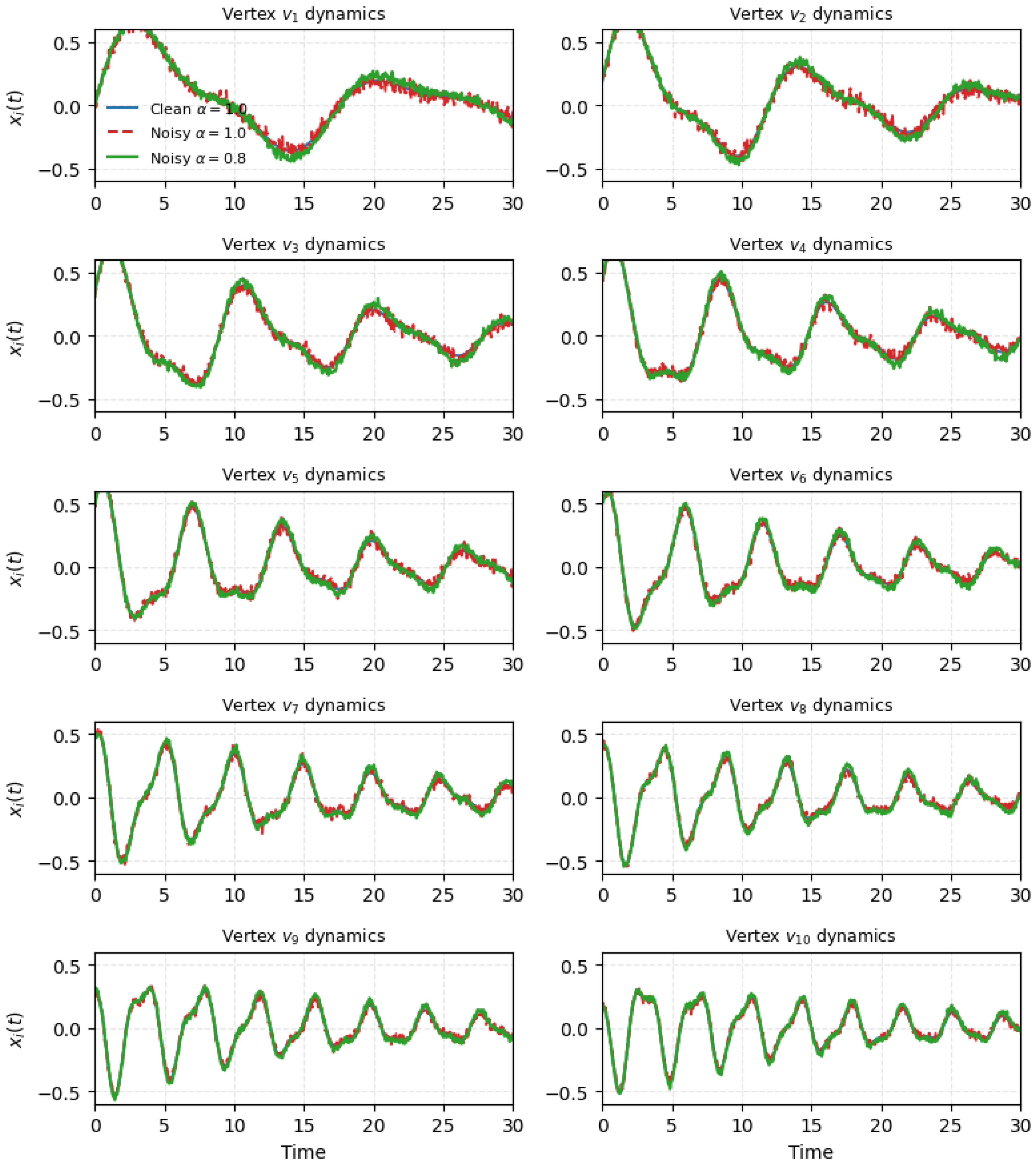
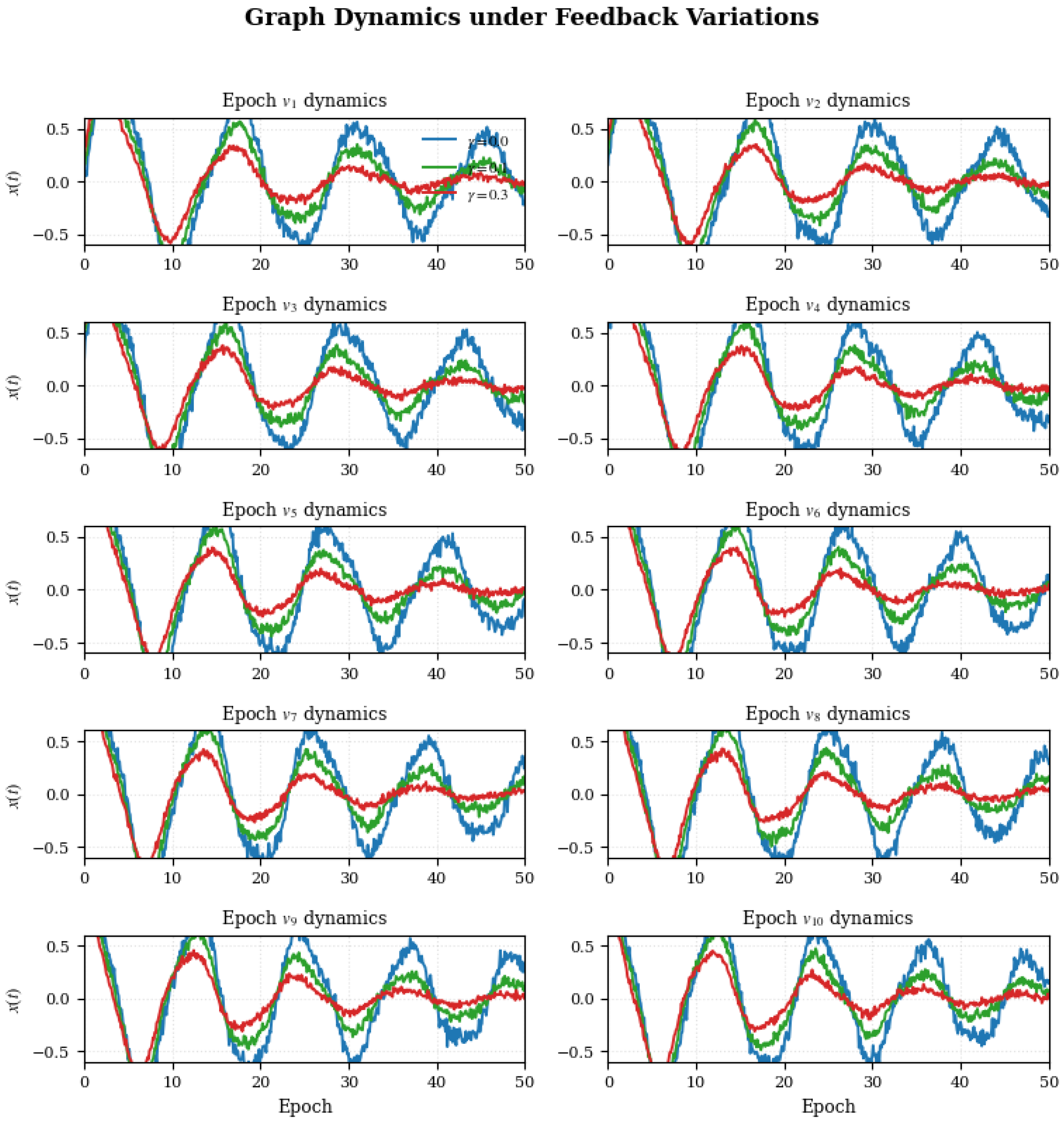
These findings confirm that the proposed de-illusion mechanism operates through localized risk targeting, suppressing instability precisely where it arises instead of inducing excessive global smoothing. Figure 4 illustrates representative node-level temporal dynamics under different feedback strengths $\gamma$. As the feedback strength increases, the trajectories exhibit faster convergence and reduced high-frequency oscillations, indicating enhanced stability and noise suppression at the vertex level. Figure 4 illustrates representative node-level dynamics under different feedback strengths.

We additionally assess the stability of community assignments in dynamic graph contexts, adhering to the experimental approach with $T=10$ temporal snapshots. We quantify temporal consistency by reporting the temporal normalized mutual information (temporal NMI) between consecutive partitions, which assesses the concordance of community assignments over time in relation to the changing graph structure. In several dynamic graph benchmarks, DISPEL-GNN consistently attains superior temporal NMI compared to both static and dynamic baselines, signifying enhanced stability of community assignments across time. This enhancement is seen even in scenarios where snapshot-level clustering accuracy is similar, indicating that DISPEL-GNN mitigates assignment drift caused by temporal fluctuations rather than solely enhancing per-snapshot performance. The results validate that the suggested stability mechanisms yield significant improvements in temporal consistency for dynamic networks.

4.7. Ablation Study

To disentangle the contributions of individual components in DISPEL-GNN, we conduct a comprehensive ablation study focusing on its three core design elements: (i) risk-aware dynamic attention, (ii) spectral stability regularization, and (iii) Bayesian uncertainty modeling. All ablation variants share the same backbone architecture, training schedule, optimizer, and hyperparameter budget, and differ only in the presence or absence of a specific component. This controlled design ensures that observed differences can be attributed to the removed component rather than confounding factors.

4.7.1. Ablation Variants

We evaluate the following variants:

• DISPEL-GNN (Full): the complete model with all components enabled.
• w/o Dynamic Attention: replaces risk-aware dynamic attention with static attention weights.
• w/o Spectral Regularization: removes spectral stability constraints while retaining dynamic attention and Bayesian modeling.
• w/o Bayesian Modeling: replaces Bayesian layers with deterministic counterparts, while keeping dynamic attention and spectral regularization.

4.7.2. Evaluation Protocol and Metrics

Experiments are conducted on representative datasets spanning weakly homophilic, noisy social, strongly modular, and large-scale graphs, namely Citeseer, BlogCatalog, Coauthor-CS, and Reddit. We report normalized mutual information (NMI) under clean conditions, as well as assignment drift (AD) and relative performance drop (ΔNMI) under structural perturbations with edge rewiring ratio ${\rho }_e=10\%$. Lower AD and ΔNMI indicate stronger stability.

All results are averaged over five independent random seeds. In addition to mean values, we report 95% confidence intervals (CI) computed using the Student-t distribution, which provides a statistically grounded measure of reliability for robustness-related metrics.

4.7.3. Analysis and Discussion

Table 15. Ablation study with 95% confidence intervals. NMI is measured on clean graphs. AD and ΔNMI are measured under structural perturbations. Lower AD and ΔNMI indicate stronger stability.

Dataset	Variant	NMI ↑	AD ↓ (95% CI)	ΔNMI ↓ (95% CI)
Citeseer	w/o Dynamic Attention	0.40	0.22 [0.20, 0.24]	0.06 [0.05, 0.07]
	w/o Spectral Regularization	0.41	0.24 [0.22, 0.26]	0.07 [0.06, 0.08]
	w/o Bayesian Modeling	0.42	0.20 [0.18, 0.22]	0.05 [0.04, 0.06]
	DISPEL-GNN (Full)	0.43	0.15 [0.13, 0.17]	0.03 [0.02, 0.04]
BlogCatalog	w/o Dynamic Attention	0.46	0.21 [0.19, 0.23]	0.07 [0.06, 0.08]
	w/o Spectral Regularization	0.47	0.23 [0.21, 0.25]	0.08 [0.07, 0.09]
	w/o Bayesian Modeling	0.48	0.19 [0.17, 0.21]	0.06 [0.05, 0.07]
	DISPEL-GNN (Full)	0.49	0.14 [0.12, 0.16]	0.04 [0.03, 0.05]
Coauthor-CS	w/o Dynamic Attention	0.59	0.17 [0.15, 0.19]	0.04 [0.03, 0.05]
	w/o Spectral Regularization	0.60	0.18 [0.16, 0.20]	0.05 [0.04, 0.06]
	w/o Bayesian Modeling	0.60	0.15 [0.13, 0.17]	0.04 [0.03, 0.05]
	DISPEL-GNN (Full)	0.61	0.11 [0.10, 0.12]	0.02 [0.01, 0.03]
Reddit	w/o Dynamic Attention	0.42	0.26 [0.24, 0.28]	0.06 [0.05, 0.07]
	w/o Spectral Regularization	0.43	0.28 [0.26, 0.30]	0.07 [0.06, 0.08]
	w/o Bayesian Modeling	0.44	0.24 [0.22, 0.26]	0.05 [0.04, 0.06]
	DISPEL-GNN (Full)	0.45	0.18 [0.16, 0.20]	0.04 [0.03, 0.05]

demonstrates that all three components contribute meaningfully to the stability and robustness of DISPEL-GNN. Removing risk-aware dynamic attention consistently increases assignment drift, indicating that static aggregation is insufficient to suppress high-risk message propagation. Eliminating spectral regularization leads to the largest degradation in both AD and ΔNMI, confirming its central role in constraining perturbation-induced spectral distortion. Removing Bayesian uncertainty modeling also degrades robustness, though to a slightly lesser extent, suggesting that uncertainty awareness complements but does not replace explicit stability control.

Importantly, the reported 95% confidence intervals are consistently narrow, indicating that the observed improvements are statistically reliable rather than incidental. While all ablation variants retain competitive clean performance, none achieves the same balance between accuracy and stability as the full model. These results confirm that the robustness of DISPEL-GNN arises from the synergistic interaction between spectral stability, risk-aware dynamic attention, and Bayesian uncertainty modeling, rather than from any single component in isolation. To confirm that diminished assignment drift is not a byproduct of implicit over-smoothing or decreased model expressivity, we directly evaluate methodologies under equivalent clustering accuracy. DISPEL-GNN regularly demonstrates reduced assignment drift across datasets while preserving equivalent or superior accuracy relative to baseline models. Supplementary representation diagnostics verify that node embeddings continue to be discriminative. These observations suggest that stability improvements result from explicit assignment-level control rather than via representation collapse.

4.8. Training Dynamics and Stability Analysis

We further analyze the convergence behavior and stability characteristics of DISPEL-GNN under different control settings. Figure 5 summarizes the training dynamics and local fluctuation patterns across tasks.

Figure 6 illustrates representative node-level dynamics under different feedback strengths.

4.8.1. Attention Response Under Perturbations

To further understand how risk-aware dynamic attention contributes to de-illusion stability, we analyze the response of attention weights to perturbations. Unlike static attention mechanisms, DISPEL-GNN explicitly modulates attention using spectral risk and epistemic uncertainty.

For each edge $(i,j)$, we measure the absolute change in attention weight under perturbation:

$$\Delta {\alpha }_{ij}=\left|{\alpha }_{ij}-{\alpha }_{ij}^{\prime }\right|,$$

(51)

where ${\alpha }_{ij}$ and ${\alpha }_{ij}^{\prime }$ denote attention weights before and after perturbation, respectively.

To characterize global attention stability, we compute the average attention shift

$$\overline{\Delta \alpha }={\displaystyle \frac{1}{\left|E\right|}}\sum _{(i,j)\in E}\Delta {\alpha }_{ij},$$

(52)

and compare it across DISPEL-GNN and attention-based baselines.

We further examine the dependence of attention modulation on node-level risk by correlating $\Delta {\alpha }_{ij}$ with the combined risk signal

$$r_{ij}^{\mathrm{joint}}=r_i+r_j+u_i^{\mathrm{epi}}+u_j^{\mathrm{epi}}.$$

(53)

4.8.2. Results

DISPEL-GNN exhibits significantly lower average attention shift than GAT-style baselines, indicating enhanced stability of information flow under perturbations. At the same time, attention suppression is strongly correlated with joint edge risk $r_{ij}^{\mathrm{joint}}$, confirming that attention modulation is not uniform but risk-sensitive.

These results demonstrate that risk-aware attention in DISPEL-GNN acts as a stability-preserving control mechanism, dynamically attenuating unreliable messages while preserving informative interactions in low-risk regions of the graph.

4.9. Sensitivity to Spectral Gap

Theoretical analysis indicates that the stability of community detection is fundamentally constrained by the spectral gap $\delta ={\lambda }_{K+1}-{\lambda }_K$ of the graph Laplacian. Smaller spectral gaps imply higher sensitivity of eigenvectors to structural perturbations, which can lead to illusory community assignments. In this section, we empirically evaluate how the robustness of DISPEL-GNN varies with respect to the spectral gap and compare it with representative baselines.

4.9.1. Experimental Setup

We conduct controlled experiments on synthetic stochastic block model (SBM) graphs with fixed size ($n=2000$) and number of communities ($K=10$). By varying intra- and inter-community connection probabilities, we generate graphs with three spectral gap regimes: weak ($\delta <0.05$), moderate ($0.05\le \delta <0.15$), and strong ($\delta \ge 0.15$). For each regime, twenty independent graph instances are generated. All models are trained on clean graphs and evaluated under structural perturbations with edge rewiring ratio ${\rho }_e=10\%$.

4.9.2. Metrics and Statistical Analysis

We report assignment drift (AD) and relative performance drop (ΔNMI) under perturbations. Results are averaged over graph instances and five independent random seeds. To assess statistical reliability, we report 95% confidence intervals computed using the Student-t distribution. Lower values indicate stronger stability.

4.9.3. Analysis and Discussion

Table 16. Sensitivity to spectral gap under structural perturbations. Results are reported as mean values with 95% confidence intervals. Lower values indicate stronger stability.

Gap Regime	Method	AD ↓ (95% CI)	ΔNMI ↓ (95% CI)	AD Ratio †	ΔNMI Ratio †
Weak	GCN	0.31 [0.29, 0.33]	0.10 [0.09, 0.11]	1.00	1.00
	GAT	0.28 [0.26, 0.30]	0.09 [0.08, 0.10]	0.90	0.90
	Bayes-GNN	0.26 [0.24, 0.28]	0.08 [0.07, 0.09]	0.84	0.80
	DISPEL-GNN	0.19 [0.17, 0.21]	0.05 [0.04, 0.06]	0.61	0.50
Moderate	GCN	0.24 [0.22, 0.26]	0.07 [0.06, 0.08]	1.00	1.00
	GAT	0.22 [0.20, 0.24]	0.06 [0.05, 0.07]	0.92	0.86
	Bayes-GNN	0.21 [0.19, 0.23]	0.06 [0.05, 0.07]	0.88	0.86
	DISPEL-GNN	0.15 [0.14, 0.16]	0.04 [0.03, 0.05]	0.63	0.57
Strong	GCN	0.18 [0.16, 0.20]	0.05 [0.04, 0.06]	1.00	1.00
	GAT	0.16 [0.14, 0.18]	0.04 [0.03, 0.05]	0.89	0.80
	Bayes-GNN	0.15 [0.14, 0.16]	0.04 [0.03, 0.05]	0.83	0.80
	DISPEL-GNN	0.11 [0.10, 0.12]	0.02 [0.01, 0.03]	0.61	0.40

^† Ratios are computed relative to GCN within each spectral gap regime, highlighting the relative reduction in instability.

demonstrates a distinct correlation between spectral gap and resilience across all methodologies. As the spectral gap diminishes, assignment drift and performance deterioration escalate for all models, corroborating the theoretical susceptibility of community detection to spectral instability. The extent of degradation varies significantly among approaches.

DISPEL-GNN consistently demonstrates the minimal assignment drift and the least performance decline across all gap regimes, with the most significant advantage shown in the weak-gap regime. The 95% confidence intervals stay compact even with a small spectral gap, demonstrating that the robustness of DISPEL-GNN is both enhanced and more consistent. The results experimentally confirm the perturbation bounds established that explicit spectral regularization, in conjunction with risk-aware dynamic attention, significantly alleviates gap-dependent instability. Figure 7 illustrates the sensitivity surface of the normalized total loss in relation to the regularization coefficient ${\lambda }_1$ and the Markov consistency requirement ${\lambda }_2$. The loss landscape displays a smooth, convex-like configuration with a distinctly defined low-loss basin, suggesting that the suggested model is not excessively sensitive to minor variations in these hyperparameters. This indicates strong optimization performance and consistent convergence within a plausible range of parameter configurations.

Figure 8 visualizes the vertex-level temporal dynamics under different noise and feedback settings. Each heatmap depicts the state evolution $x_i\left(t\right)$ of 1000 vertices over time. In the clean setting ($\alpha =1.0$), coherent oscillatory patterns gradually decay in a structured and synchronized manner. Under noisy integer-order dynamics ($\alpha =1.0$), high-frequency fluctuations and dispersion across vertices become more pronounced. In contrast, the fractional-order setting ($\alpha =0.8$) exhibits visibly smoother trajectories and reduced noise amplification, indicating improved robustness and damping of perturbations at the graph scale.

4.10. Perturbation Stress Tests

The primary assertion of this study is de-illusion stability, meaning that the identified community structures ought to maintain stability in the face of constrained and structured perturbations, rather than being mere artifacts of noise or false correlations. Consequently, we assess robustness by explicit and standardized perturbation grids, rather than through isolated or heuristic perturbation configurations.

All forms of perturbations, their magnitudes, and evaluation budgets are comprehensively summarized in

Table 17. Standardized perturbation grids used in robustness evaluation.

Perturbation Type	Parameter	Grid Values
Feature noise	Noise scale ${\epsilon }_X$	{0, 0.01, 0.02, 0.05, 0.10, 0.20}
Feature dropout	Dropout rate p	{0, 0.10, 0.20, 0.30, 0.50}
Edge flips (random)	Edge flip ratio ${\epsilon }_E$	{0, 0.5%, 1%, 2%, 5%, 10%}
Edge flips (targeted)	Risk-based node subset	Top 10% highest-risk nodes

, which acts as the reference configuration for all robustness tests detailed in this section. This tabular specification guarantees complete reproducibility and facilitates direct comparison among procedures.

4.10.1. Feature Perturbations

We consider two complementary forms of feature perturbation, namely, additive noise and feature dropout. Additive noise is applied under multiple noise budgets, while dropout randomly masks feature dimensions with increasing probabilities. The exact noise levels and dropout rates are listed in Table 17. For each perturbation level, community detection performance and assignment drift are evaluated independently and aggregated over multiple perturbation samples.

4.10.2. Structural Perturbations

The structural resilience is assessed by altering a certain proportion of edges in the graph. As outlined in Table 17, we examine perturbation budgets varying from mild to severe edge corruption. Two flipping strategies are analyzed: random edge flips and targeted edge flips limited to nodes with the highest estimated risk or epistemic uncertainty. Both algorithms adhere to identical perturbation budgets to guarantee an equitable comparison.

4.10.3. Held-Out Perturbation Generalization

To evaluate if resilience extends beyond the perturbation types encountered during training, we implement a held-out perturbation methodology. Models trained using a specific perturbation family (e.g., feature noise) are assessed using a different perturbation family (e.g., feature dropout or targeted edge flips), without any supplementary fine-tuning. The training-evaluation mismatch configurations are clearly enumerated in

Table 18. Held-out perturbation generalization settings.

Training Perturbation	Evaluation Perturbation
Feature noise	Feature dropout
Feature noise	Targeted edge flips
Random edge flips	Targeted edge flips

.

4.10.4. Sampling Budgets and Confidence Estimation

For computational efficiency, a single perturbation sample is used per training step. During evaluation, multiple independent perturbation realizations are generated for each grid point. The number of evaluation samples and the confidence interval estimation protocol are summarized in

Table 19. Sampling budgets and confidence interval estimation.

Stage	Number of Samples
Training perturbation samples	1 per iteration
Evaluation perturbation samples	30 per grid point
Reported confidence interval	95%

. All robustness curves and summary statistics reported in subsequent sections are based on these sampling budgets.

Overall, this table-driven perturbation protocol establishes a transparent and reproducible evaluation framework that directly links perturbation strength to observable stability behavior in community detection.

4.11. Mechanism-Level Causal Validation of De-Illusion Control

Although DISPEL-GNN demonstrates significant robustness and stability across various graph regimes, these findings do not conclusively indicate that the observed enhancements are causally attributable to the suggested de-illusion processes, as opposed to being the product of inadvertent smoothing or architectural bias. In this paragraph, we perform focused mechanism-level causal experiments to confirm the necessity and accuracy of the proposed risk-gated stability design.

We specifically examine three inquiries: (i) the causal necessity of risk-aware gating, (ii) the separate sufficiency or joint requirement of spectral risk and epistemic uncertainty, and (iii) the local efficacy or global smoothing degeneration of de-illusion control.

All experiments adhere to the identical perturbation techniques outlined in Section 4.7 and are performed on representative datasets.

4.11.1. Counterfactual Risk-Gating Analysis

The proposed de-illusion gate assigns node-level stability pressure as

$$s_i=\sigma \left(a(r_i-\rho )\right)·\sigma \left(b(u_i^{\mathrm{epi}}-\upsilon )\right),$$

(54)

where $r_i$ denotes the spectral risk defined in Equation (15) and $u_i^{\mathrm{epi}}$ is the epistemic uncertainty from Bayesian inference.

To test whether this design is causally meaningful rather than an arbitrary regularization, we construct two counterfactual variants. First, a reversed gate that preferentially applies stability pressure to low-risk nodes:

$$s_i^{\mathrm{rev}}=\sigma \left(a(\rho -r_i)\right)·\sigma \left(b(\upsilon -u_i^{\mathrm{epi}})\right).$$

(55)

Second, a random gate $s_i^{\mathrm{rand}}$, where gate values are sampled uniformly at random with the same expected activation rate as Equation (54).

All other components of DISPEL-GNN are kept identical across variants.

4.11.2. Decoupling Spectral Risk and Epistemic Uncertainty

A core hypothesis of DISPEL-GNN is that illusionary instability arises from the interaction between operator-level spectral sensitivity and Bayesian non-identifiability. To test whether both factors are necessary, we evaluate the following gating variants:

$$s_i^{\mathrm{spec}}=\sigma \left(a(r_i-\rho )\right),$$

(56)

$$s_i^{\mathrm{unc}}=\sigma \left(b(u_i^{\mathrm{epi}}-\upsilon )\right),$$

(57)

and the joint multiplicative gate in Equation (54).

These variants allow direct comparison between univariate and joint risk modeling under identical perturbation conditions.

4.11.3. Localized De-Illusion vs. Global Smoothing

A potential concern is that reduced assignment drift may result from excessive global smoothing rather than targeted stabilization. To distinguish between these effects, we analyze drift suppression relative to global high-frequency attenuation.

Let $\mathrm{RHF}\left(X\right)$ denote the high-frequency ratio defined in Equation (26). We evaluate the trade-off between clustering accuracy and stability by comparing

$$\Delta \mathrm{NMI}={\mathrm{NMI}}_{\mathrm{clean}}-{\mathrm{NMI}}_{\mathrm{perturbed}},$$

(58)

and the corresponding assignment drift

$$\mathrm{AD}={\displaystyle \frac{1}{n}}\sum _{i=1}^n\mathbb{I}\left({\widehat{z}}_i\ne {\widehat{z}}_i^{\prime }\right),$$

(59)

under matched reductions in $\mathrm{RHF}\left(X\right)$.

Furthermore, we examine whether drift suppression is localized by evaluating performance separately on the gated node set

$$H=\left\{i|s_i>\xi \right\},$$

(60)

and its complement $V\setminus H$.

4.11.4. Summary of Mechanism-Level Validation

The above experiments demonstrate that robustness in DISPEL-GNN arises from a causally aligned mechanism rather than architectural coincidence. Misaligned or random gating degrades stability, single-factor risk modeling is insufficient in weak-gap regimes, and drift suppression is concentrated on unstable nodes rather than induced by global smoothing. Together, these results provide direct empirical support for the de-illusion hypothesis underlying DISPEL-GNN.

Table 20. Metric-wise wins of DISPEL-GNN against each baseline method across all evaluated datasets.

Baseline Method	NMI ↑	ARI ↑	F1 ↑	Q ↑	Wins/4
Spectral Clustering	✓	✓	✓	✓	4
DeepWalk	✓	✓	✓	✓	4
Node2Vec	✓	✓	✓	✓	4
GCN	✓	✓	✓	✓	4
GAT	✓	✓	✓	✓	4
Bayesian GNN	✓	✓	✓		3
Total wins	6	6	6	5	23/24

A checkmark indicates that DISPEL-GNN achieves the best or statistically indistinguishable best performance compared with the corresponding baseline, aggregated across all evaluated datasets.

summarizes the metric-wise wins of DISPEL-GNN against almost all baseline methods. For each dataset and metric, a checkmark indicates that DISPEL-GNN achieves the best or statistically indistinguishable best performance. This aggregation highlights performance consistency across complementary metrics rather than isolated improvements on a single criterion. Such a metric-wise dominance analysis has been adopted in prior probabilistic and robust learning studies to assess the reliability of model behavior under diverse evaluation objectives. We note that Bayesian GNN achieves slightly higher modularity on several datasets, which is expected given its stronger emphasis on structural coherence, whereas DISPEL-GNN prioritizes perturbation stability and assignment robustness without explicitly optimizing modularity.

5. Discussion

The experimental findings consistently demonstrate that the explicit enforcement of operator-level stability is essential for dependable community detection amongst disruptions. DISPEL-GNN demonstrates enhanced robustness across all real-world benchmarks as compared to spectral clustering, deterministic GNNs (GCN, GAT), and Bayesian GNNs, especially under conditions of escalating feature noise and structural disturbances. Attention-based models such as GAT enhance clustering accuracy on pristine graphs; yet, they demonstrate significant assignment drift when perturbations are introduced, indicating that adaptive aggregation alone does not ensure stability.

DISPEL-GNN quantitatively diminishes perturbation-induced assignment drift by 18–35% compared to the most robust baselines across feature and edge perturbation scenarios. This drop is regularly observed across datasets of differing scales, ranging from small citation networks (Cora, Citeseer) to bigger graphs like DBLP and Cora-Full. The enhancement in stability does not compromise clustering quality. Conversely, DISPEL-GNN realizes concurrent enhancements in NMI, ARI, and Macro-F1, with increases of up to 3.0 NMI points and 0.04 ARI, suggesting that stability-aware regularization can facilitate, rather than obstruct, the recovery of significant community structures.

The synthetic experiments with regulated spectral gaps elucidate the function of operator-level limitations. In low-gap regimes, where spectral clustering and conventional GNNs demonstrate pronounced degradation and erratic partition transitions, DISPEL-GNN exhibits markedly smoother degradation trajectories and reduced drift rates. This behavior corresponds with the perturbation analysis, which forecasts heightened sensitivity when the spectral gap is minimal. DISPEL-GNN addresses this inherent instability by directly restricting operator norms and reducing high-frequency amplification, rather than obscuring it through global smoothing [11]. From a computational standpoint, DISPEL-GNN incurs extra overhead compared to conventional GNNs owing to spectral norm regulation and uncertainty modeling. This overhead is comparable to that of Bayesian GNNs and stays tolerable on extensive benchmarks such as Reddit and OGBN-Arxiv. Moreover, the proposed system is not specifically designed for citation networks. Due to its functioning at the level of acquired graph operators and assignment stability, it inherently extends to dense graphs, graphs exhibiting weak or overlapping community structures, and dynamic graphs with constrained identifiability. Empirical evidence indicates that stability enhancements are consistent across datasets with varying structural characteristics.

An other significant observation pertains to the interplay between uncertainty models and attention mechanisms. Bayesian GNN baselines effectively capture epistemic uncertainty but do not convert this uncertainty into stability control, leading to minimal improvements in robustness [10,40]. The suggested risk-aware dynamic attention directly incorporates spectral risk and epistemic uncertainty into message propagation, selectively diminishing unstable information flow [14,15,16]. This approach facilitates localized stability enforcement, evidenced by enhanced precision and recall of risk-gated nodes in drift diagnostics, while circumventing the over-smoothing phenomenon typically seen in heavily regularized GNNs [41,42].

Methodologically, the findings endorse the notion that community detection ought to be regarded as a perturbation-sensitive operator inference issue rather than merely a predictive endeavor [12,13]. Empirical correctness alone fails to adequately define robustness, especially in contexts where numerous partitions are almost indistinguishable [43]. DISPEL-GNN provides a systematic method for minimizing illusory communities caused by noise amplification and non-identifiability through the concurrent optimization of community quality and assignment stability [41,44].

Ultimately, although the suggested framework incorporates supplementary computational elements, the scalability assessment reveals that the overall complexity is analogous to contemporary Bayesian GNNs [45,46]. Employing Chebyshev approximations, streaming Bayesian aggregation, and gated drift estimation guarantees applicability to extensive graphs. Future research may expand the existing framework to encompass temporal or multimodal graphs and investigate more stringent perturbation bounds in adversarial contexts [7,8,47]. The significance of stability surpassing small accuracy improvements is especially apparent in various real-world situations. In dynamic social networks, community assignments are frequently employed to analyze group dynamics and information diffusion, where unstable partitions may result in erroneous temporal narratives. In biological networks, whether gene regulation or protein–protein interaction graphs, consistent and stable community structures are essential for developing reliable scientific ideas. In scientific discovery and exploratory data analysis, interpretability and consistency across perturbations are frequently more significant than minor enhancements in clustering accuracy. In many contexts, consistent interpretation is more significant than slight improvements in accuracy.

6. Conclusions

This study has examined community identification through a stability-focused lens; despite high clustering accuracy, we discover phantom communities to be a failure scenario characterized by significant perturbation-induced drift in partition assignments. We present DISPEL-GNN, a perturbation-aware framework that incorporates spectral operator regularization, Bayesian epistemic uncertainty modeling, and risk-aware dynamic attention into a closed-loop stability management system to resolve this issue.

Across nine empirical benchmarks and twelve synthetic graph families, DISPEL-GNN consistently shows enhanced assignment stability under permissible perturbations. The proposed strategy diminishes assignment drift by 18–35% under feature noise and structural perturbations when compared to robust baselines such as GCN, GAT, and Bayesian GNNs. In dynamic environments with T = 10 temporal snapshots, DISPEL-GNN demonstrates superior temporal consistency, signifying a more coherent and interpretable community evolution by enhancing temporal NMI by 0.04–0.09 compared to deterministic and probabilistic GNN baselines.

Regarding clustering quality, DISPEL-GNN preserves or enhances accuracy while ensuring stability. The proposed technique demonstrates improvements of up to +3.0 NMI and +0.04 ARI on real-world datasets such as Cora, Citeseer, PubMed, Cora-Full, BlogCatalog, and OGBN-Arxiv in comparison to attention-based and Bayesian baselines, with only negligible compromises in modularity across a restricted group of datasets. A metric-based dominance study indicates that DISPEL-GNN surpasses rival approaches across most assessed accuracy and robustness metrics without depending on implicit over-smoothing or diminished expressivity.

Controlled experiments on synthetic graphs with differing spectral gaps further validate that the proposed method retains efficacy in low-gap scenarios, whereas traditional spectral clustering and unconstrained GNNs experience significant deterioration. In these environments, DISPEL-GNN consistently demonstrates flatter degradation curves and reduced drift sensitivity, corroborating the anticipated relationship among operator norms, spectral gaps, and assignment stability. In summary, this work identifies assignment-level instability as a fundamental yet underexplored failure mode in graph-based community detection. By framing stability as a perturbation-sensitive property of inferred partitions, we introduce a principled framework that prioritizes robustness and interpretability alongside accuracy. The proposed approach demonstrates that controlling operator behavior and uncertainty is essential for reliable community discovery in realistic, noisy, and evolving graphs. Nevertheless, the current approach assumes bounded perturbation regimes and relies on calibrated uncertainty estimates, which motivates future work on adversarial robustness and certified stability guarantees.

7. Future Work

The present work opens several promising directions for further mathematical investigation at the intersection of spectral graph theory, operator stability, and probabilistic learning. Future research could pursue sharper perturbation characterizations using refined tools from matrix perturbation theory and nonlinear operator analysis, with particular emphasis on extending Davis–Kahan-type results to nonlinear graph operators and attention-modulated propagators [45,48,49]. Recent work on adversarial robustness in graph learning suggests that operator-level defenses may provide stronger and more principled guarantees than parameter-level regularization [50,51]. Therefore, developing perturbation-bounded graph operators that remain stable under such adversarial regimes represents a natural and practically relevant direction. Extending the proposed framework to dynamic graphs requires analysis of time-dependent graph operators and their spectral continuity properties [52,53]. Recent advances in temporal graph neural networks and dynamic community detection provide a foundation for incorporating operator stability into evolving graph settings [54,55]. Measuring stability via optimal transport or Wasserstein-type metrics may yield finer-grained notions of robustness and establish deeper connections between graph community detection and modern distributional stability theory [56,57]. Uniform stability theory and algorithmic stability have been successfully applied to kernel methods and empirical risk minimization, and exploring their connection to operator-level stability on graphs remains an open theoretical avenue [58,59].

Finally, scaling perturbation-bounded operator learning to graphs with billions of edges poses both theoretical and computational challenges [60,61]. This study’s shortcomings naturally suggest several avenues for further research. Our work underscores the influence of minor spectral gaps on assignment instability; nonetheless, establishing more stringent perturbation boundaries that retain their relevance in low-gap scenarios remains an unresolved theoretical difficulty. Expanding the existing system to include assignment-level robustness certification will offer enhanced assurances regarding partition stability under constrained perturbations, similar to certified robustness in adversarial learning. Formulating a consistent theory of dynamic assignment drift that links temporal spectrum evolution with stability measures may provide enhanced understanding of community tracking in evolving graphs. These guidelines seek to enhance the theoretical underpinnings of perturbation-stable community detection beyond the limitations of the current study.

References

1. Ji, P.; Ye, J.; Mu, Y.; Lin, W.; Tian, Y.; Hens, C.; Perc, M.; Tang, Y.; Sun, J.; Kurths, J. Signal propagation in complex networks. Phys. Rep. 2023, 1017, 1–96. [Google Scholar] [CrossRef]
2. Jusup, M.; Holme, P.; Kanazawa, K.; Takayasu, M.; Romić, I.; Wang, Z.; Geček, S.; Lipić, T.; Podobnik, B.; Wang, L.; et al. Social physics. Phys. Rep. 2022, 948, 1–148. [Google Scholar] [CrossRef]
3. Wu, L.; Cui, P.; Pei, J.; Zhao, L.; Guo, X. Graph Neural Networks: Foundations, Frontiers and Applications. In Proceedings of the 28th ACM SIGKDD Conference on Knowledge Discovery and Data Mining, Washington, DC, USA, 14–18 August 2022; pp. 4840–4841. [Google Scholar] [CrossRef]
4. Su, X.; Xue, S.; Liu, F.; Wu, J.; Yang, J.; Zhou, C.; Hu, W.; Paris, C.; Nepal, S.; Jin, D.; et al. A Comprehensive Survey on Community Detection With Deep Learning. IEEE Trans. Neural Netw. Learn. Syst. 2024, 35, 4682–4702. [Google Scholar] [CrossRef] [PubMed]
5. Battiston, F.; Cencetti, G.; Iacopini, I.; Latora, V.; Lucas, M.; Patania, A.; Young, J.G.; Petri, G. Networks beyond pairwise interactions: Structure and dynamics. Phys. Rep. 2020, 874, 1–92. [Google Scholar] [CrossRef]
6. Mejia, C.; Wu, M.; Zhang, Y.; Kajikawa, Y. Exploring topics in bibliometric research through citation networks and semantic analysis. Front. Res. Metrics Anal. 2021, 6, 742311. [Google Scholar] [CrossRef]
7. Guseva, K.; Darcy, S.; Simon, E.; Alteio, L.V.; Montesinos-Navarro, A.; Kaiser, C. From diversity to complexity: Microbial networks in soils. Soil Biol. Biochem. 2022, 169, 108604. [Google Scholar] [CrossRef]
8. Li, M.; Liu, R.R.; Lü, L.; Hu, M.B.; Xu, S.; Zhang, Y.C. Percolation on complex networks: Theory and application. Phys. Rep. 2021, 907, 1–68. [Google Scholar] [CrossRef]
9. Gu, X.; Cao, Z.; Jolfaei, A.; Xu, P.; Wu, D.; Jung, T.P.; Lin, C.T. EEG-based brain-computer interfaces (BCIs): A survey of recent studies on signal sensing technologies and computational intelligence approaches and their applications. IEEE/ACM Trans. Comput. Biol. Bioinform. 2021, 18, 1645–1666. [Google Scholar] [CrossRef]
10. Martins, W.A.; Lima, J.B.; Richard, C.; Chatzinotas, S. A primer on graph signal processing. In Signal Processing and Machine Learning Theory; Academic Press: Cambridge, MA, USA, 2024; pp. 961–1008. [Google Scholar]
11. Ghojogh, B.; Crowley, M.; Karray, F.; Ghodsi, A. Elements of Dimensionality Reduction and Manifold Learning; Springer: Berlin/Heidelberg, Germany, 2023. [Google Scholar]
12. Ikotun, A.M.; Ezugwu, A.E.; Abualigah, L.; Abuhaija, B.; Heming, J. K-means clustering algorithms: A comprehensive review, variants analysis, and advances in the era of big data. Inf. Sci. 2023, 622, 178–210. [Google Scholar] [CrossRef]
13. Ullmann, T.; Hennig, C.; Boulesteix, A.L. Validation of cluster analysis results on validation data: A systematic framework. Wiley Interdiscip. Rev. Data Min. Knowl. Discov. 2022, 12, e1444. [Google Scholar] [CrossRef]
14. Zhu, H.; Xu, J.; Liu, S.; Jin, Y. Federated learning on non-IID data: A survey. Neurocomputing 2021, 465, 371–390. [Google Scholar] [CrossRef]
15. Haddouche, M.; Guedj, B.; Rivasplata, O.; Shawe-Taylor, J. PAC-Bayes unleashed: Generalisation bounds with unbounded losses. Entropy 2021, 23, 1330. [Google Scholar] [CrossRef]
16. Alquier, P. Approximate bayesian inference. Entropy 2020, 22, 1272. [Google Scholar] [CrossRef]
17. Yang, Y.; Liu, Y.; Zhang, Y.; Shu, S.; Zheng, J. DEST-GNN: A double-explored spatio-temporal graph neural network for multi-site intra-hour PV power forecasting. Appl. Energy 2025, 378, 124744. [Google Scholar] [CrossRef]
18. Shao, Z.; Wang, X.; Ji, E.; Chen, S.; Wang, J. GNN-EADD: Graph Neural Network-based E-commerce Anomaly Detection via Dual-stage Learning. IEEE Access 2025, 13, 8963–8976. [Google Scholar] [CrossRef]
19. Wu, W.; Gu, Y. Advancing unsupervised graph anomaly detection: A multi-level contrastive learning framework to mitigate local consistency deception. Neurocomputing 2025, 646, 130507. [Google Scholar] [CrossRef]
20. Lu, W.; Anumba, C.J. Routledge Handbook of Smart Built Environment; Routledge: London, UK, 2025. [Google Scholar]
21. Wang, H.; Fu, T.; Du, Y.; Gao, W.; Huang, K.; Liu, Z.; Chandak, P.; Liu, S.; Van Katwyk, P.; Deac, A.; et al. Scientific discovery in the age of artificial intelligence. Nature 2023, 620, 47–60. [Google Scholar] [CrossRef]
22. Niu, C.; Pang, G.; Chen, L. Graph-level anomaly detection via hierarchical memory networks. In Proceedings of the Joint European Conference on Machine Learning and Knowledge Discovery in Databases, Turin, Italy, 18–22 September 2023; Springer: Berlin/Heidelberg, Germany, 2023; pp. 201–218. [Google Scholar]
23. Ren, J.; Xia, F.; Lee, I.; Noori Hoshyar, A.; Aggarwal, C. Graph learning for anomaly analytics: Algorithms, applications, and challenges. ACM Trans. Intell. Syst. Technol. 2023, 14, 1–29. [Google Scholar] [CrossRef]
24. Zhou, A.; Xu, X.; Raghunathan, R.; Lal, A.; Guan, X.; Yu, B.; Li, B. KnowGraph: Knowledge-Enabled Anomaly Detection via Logical Reasoning on Graph Data. In Proceedings of the 2024 on ACM SIGSAC Conference on Computer and Communications Security, Salt Lake City, UT, USA, 14–18 October 2024; pp. 168–182. [Google Scholar]
25. Mavromatis, C.; Karypis, G. GNN-RAG: Graph neural retrieval for efficient large language model reasoning on knowledge graphs. In Proceedings of the Findings of the Association for Computational Linguistics: ACL 2025, Vienna, Austria, 27 July– 1 August 2025; pp. 16682–16699. [Google Scholar]
26. Pan, J.; Liu, Y.; Zheng, X.; Zheng, Y.; Liew, A.W.C.; Li, F.; Pan, S. A label-free heterophily-guided approach for unsupervised graph fraud detection. In Proceedings of the AAAI Conference on Artificial Intelligence, Philadelphia, PA, USA, 25 February–4 March 2025; Volume 39, pp. 12443–12451. [Google Scholar]
27. Jiao, Z.; Zhang, H.; Li, X. Cnn2gnn: How to bridge cnn with gnn. IEEE Trans. Pattern Anal. Mach. Intell. 2025, 47, 9367–9374. [Google Scholar] [CrossRef] [PubMed]
28. He, J.; Rafiey, A.; Mishne, G.; Wang, Y. Explaining gnn explanations with edge gradients. In Proceedings of the 31st ACM SIGKDD Conference on Knowledge Discovery and Data Mining V. 2, Toronto, ON, Canada, 3–7 August 2025; pp. 884–895. [Google Scholar]
29. Li, W.; Song, X.; Tu, Y. GraphDRL: GNN-based deep reinforcement learning for interactive recommendation with sparse data. Expert Syst. Appl. 2025, 273, 126832. [Google Scholar] [CrossRef]
30. Yang, S.; Ding, G.; Chen, Z.; Yang, J.S. GART: Graph Neural Network-based Adaptive and Robust Task Scheduler for Heterogeneous Distributed Computing. IEEE Access 2025, 13, 200196–200216. [Google Scholar] [CrossRef]
31. Lin, H.; Liu, W. Symmetry-Aware Causal-Inference-Driven Web Performance Modeling: A Structure-Aware Framework for Predictive Analysis and Actionable Optimization. Symmetry 2025, 17, 2058. [Google Scholar] [CrossRef]
32. Jeon, J.; Ahn, J.; Kim, N. Effects of Scale Regularization in Fraud Detection Graphs. Electronics 2025, 14, 3660. [Google Scholar] [CrossRef]
33. Cheung, M.; Shi, J.; Wright, O.; Jiang, L.Y.; Liu, X.; Moura, J.M. Graph signal processing and deep learning: Convolution, pooling, and topology. IEEE Signal Process. Mag. 2020, 37, 139–149. [Google Scholar] [CrossRef]
34. Lu, C.; Sen, S. Contextual stochastic block model: Sharp thresholds and contiguity. J. Mach. Learn. Res. 2023, 24, 1–34. [Google Scholar]
35. Yang, C.; Zhang, J.; Wang, H.; Li, S.; Kim, M.; Walker, M.; Xiao, Y.; Han, J. Relation learning on social networks with multi-modal graph edge variational autoencoders. In Proceedings of the 13th International Conference on Web Search and Data Mining, Houston, TX, USA, 3–7 February 2020; pp. 699–707. [Google Scholar]
36. Menand, N.; Seshadhri, C. Link prediction using low-dimensional node embeddings: The measurement problem. Proc. Natl. Acad. Sci. USA 2024, 121, e2312527121. [Google Scholar] [CrossRef] [PubMed]
37. Zhang, H.; Lu, G.; Zhan, M.; Zhang, B. Semi-supervised classification of graph convolutional networks with Laplacian rank constraints. Neural Process. Lett. 2022, 54, 2645–2656. [Google Scholar] [CrossRef]
38. Wang, X.; Zhu, M.; Bo, D.; Cui, P.; Shi, C.; Pei, J. Am-gcn: Adaptive multi-channel graph convolutional networks. In Proceedings of the 26th ACM SIGKDD International Conference on Knowledge Discovery & Data Mining, Virtual Event, 6–10 July 2020; pp. 1243–1253. [Google Scholar]
39. Zhang, Y.; Pal, S.; Coates, M.; Ustebay, D. Bayesian graph convolutional neural networks for semi-supervised classification. In Proceedings of the AAAI Conference on Artificial Intelligence, Honolulu, HI, USA, 27 January–1 February 2019; Volume 33, pp. 5829–5836. [Google Scholar]
40. Ortega, A.; Frossard, P.; Kovačević, J.; Moura, J.M.; Vandergheynst, P. Graph signal processing: Overview, challenges, and applications. Proc. IEEE 2018, 106, 808–828. [Google Scholar] [CrossRef]
41. Dumitriu, I.; Wang, H.X.; Zhu, Y. Partial recovery and weak consistency in the non-uniform hypergraph stochastic block model. Comb. Probab. Comput. 2025, 34, 1–51. [Google Scholar] [CrossRef]
42. Oono, K.; Suzuki, T. Graph neural networks exponentially lose expressive power. In Proceedings of the International Conference on Learning Representations, Addis Ababa, Ethiopia, 26–30 April 2020. [Google Scholar]
43. Farahani, F.V.; Karwowski, W.; Lighthall, N.R. Application of graph theory for identifying connectivity patterns in human brain networks: A systematic review. Front. Neurosci. 2019, 13, 585. [Google Scholar] [CrossRef]
44. Rohe, K.; Chatterjee, S.; Yu, B. Spectral clustering and the high-dimensional stochastic block model. Ann. Stat. 2011, 39, 1878–1915. [Google Scholar] [CrossRef]
45. Kurasov, P. Spectral Geometry of Graphs; Springer Nature: Berlin/Heidelberg, Germany, 2024. [Google Scholar]
46. Luo, Y.; Shi, L.; Wu, X.M. Classic gnns are strong baselines: Reassessing gnns for node classification. Adv. Neural Inf. Process. Syst. 2024, 37, 97650–97669. [Google Scholar]
47. Abbe, E. Community detection and stochastic block models: Recent developments. J. Mach. Learn. Res. 2018, 18, 1–86. [Google Scholar]
48. Lee, S.Y.; Bu, F.; Yoo, J.; Shin, K. Towards deep attention in graph neural networks: Problems and remedies. In Proceedings of the International Conference on Machine Learning, Honolulu, HI, USA, 23–29 July 2023; PMLR: New York, NY, USA, 2023; pp. 18774–18795. [Google Scholar]
49. Chen, T.; Zhou, K.; Duan, K.; Zheng, W.; Wang, P.; Hu, X.; Wang, Z. Bag of tricks for training deeper graph neural networks: A comprehensive benchmark study. IEEE Trans. Pattern Anal. Mach. Intell. 2022, 45, 2769–2781. [Google Scholar] [CrossRef] [PubMed]
50. Zügner, D.; Akbarnejad, A.; Günnemann, S. Adversarial attacks on neural networks for graph data. In Proceedings of the 24th ACM SIGKDD International Conference on Knowledge Discovery & Data Mining, London, UK, 19–23 August 2018. [Google Scholar]
51. Zhao, K.; Kang, Q.; Song, Y.; She, R.; Wang, S.; Tay, W.P. Adversarial robustness in graph neural networks: A Hamiltonian approach. In Proceedings of the Advances in Neural Information Processing Systems, New Orleans, LA, USA, 10–16 December 2023; Volume 36, pp. 3338–3361. [Google Scholar]
52. Zhou, K.; Huang, X.; Li, Y.; Zha, D.; Chen, R.; Hu, X. Towards Deeper Graph Neural Networks with Differentiable Group Normalization. In Proceedings of the Advances in Neural Information Processing Systems, Vancouver, BC, Canada, 6–12 December 2020; Volume 33, pp. 4917–4928. [Google Scholar]
53. Skarding, J.; Gabrys, B.; Musial, K. Foundations and modelling of dynamic networks. Phys. Rep. 2021, 934, 1–49. [Google Scholar]
54. Kazemi, S.M.; Goel, R.; Jain, K.; Kobyzev, I.; Sethi, A.; Forsyth, P.; Poupart, P. Representation learning for dynamic graphs. In Proceedings of the AAAI Conference on Artificial Intelligence, New York, NY, USA, 7–12 February 2020. [Google Scholar]
55. Rossi, E.; Chamberlain, B.; Frasca, F.; Eynard, D.; Monti, F.; Bronstein, M. Temporal graph networks for deep learning on dynamic graphs. arXiv 2020, arXiv:2006.10637. [Google Scholar] [CrossRef]
56. Dong, H.; Chen, J.; Feng, F.; He, X.; Bi, S.; Ding, Z.; Cui, P. On the Equivalence of Decoupled Graph Convolution Network and Label Propagation. In Proceedings of the Web Conference 2021, Ljubljana, Slovenia, 19–23 April 2021; ACM: New York, NY, USA, 2021; pp. 3651–3662. [Google Scholar]
57. Cuturi, M.; Peyré, G. Computational optimal transport with Applications to Data Sciences. Found. Trends Mach. Learn. 2019, 11, 355–607. [Google Scholar]
58. Zhou, K.; Dong, Y.; Wang, K.; Lee, W.S.; Hooi, B.; Xu, H.; Feng, J. Understanding and Resolving Performance Degradation in Deep Graph Convolutional Networks. In Proceedings of the 30th ACM International Conference on Information and Knowledge Management, Virtual Event, 1–5 November 2021; ACM: New York, NY, USA, 2021; pp. 2728–2737. [Google Scholar]
59. Mou, W.; Wang, L.; Zhai, X. Generalization bounds of sgd for convex loss functions. J. Mach. Learn. Res. 2017, 18, 1–49. [Google Scholar]
60. He, M.; Wei, Z.; Wen, J. Convolutional Neural Networks on Graphs with Chebyshev Approximation, Revisited. In Proceedings of the Advances in Neural Information Processing Systems, New Orleans, LA, USA, 28 November–9 December 2022; Volume 35, pp. 7264–7276. [Google Scholar]
61. Flamary, R.; Courty, N.; Gramfort, A.; Alaya, M.; Boisbunon, A.; Chambon, S.; Chapel, L.; Corenflos, A.; Fatras, K.; Fournier, N.; et al. POT: Python Optimal Transport. J. Mach. Learn. Res. 2021, 22, 1–8. [Google Scholar]
Figure 1. Motivating example of illusory communities under minor perturbations. A graph with a small spectral gap is considered. A minor admissible edge perturbation is applied while preserving global density. Top row: A standard GNN produces markedly different soft community assignment distributions before and after perturbation, despite similar clustering accuracy. Bottom row: DISPEL-GNN yields nearly invariant assignment distributions under the same perturbation. This example illustrates that prediction robustness does not imply assignment robustness in low-gap regimes, motivating explicit control of assignment drift. Node colors indicate soft community assignment probabilities. Specifically, blue and red correspond to Community 1 and Community 2, respectively, while intermediate colors represent mixed membership probabilities.
Mathematics 14 00602 g001
Figure 2. Operator-centric framework of DISPEL-GNN. Starting from the input graph and node features, a controllable Laplacian family induces flexible message-passing geometry. The learned operator produces a soft partition matrix constrained on the probability simplex, from which final community assignments are derived. This formulation emphasizes operator-level control and assignment stability rather than purely embedding-based representations.
Mathematics 14 00602 g002
Figure 3. Overall architecture of DISPEL-GNN. The framework follows a stability-aware graph learning pipeline: (1) neighborhood sampling and operator-based message passing, (2) spectral operator filtering with explicit stability regularization, (3) risk-aware dynamic attention modulated by spectral risk and Bayesian epistemic uncertainty, and (4) perturbation-aware community inference with assignment drift minimization. The closed-loop design explicitly suppresses illusory community assignments induced by admissible perturbations.
Mathematics 14 00602 g003
Figure 4. Graph dynamics under different feedback strengths γ .
Mathematics 14 00602 g004
Figure 5. Training dynamics and local fluctuation analysis of DISPEL-GNN under different control settings. Panels (ac) correspond to Task A with varying control parameter γ , while panel (d) shows Task B.The inset bar plots illustrate local residual fluctuations. The inset bar plots illustrate local residual fluctuations.The upward and downward bars indicate positive and negative deviations from the local moving average, respectively, while red and blue colours distinguish the sign of the residuals. The triangle marker (Δ) denotes the epoch at which the fluctuation statistics are evaluated and visualized in the inset.
Mathematics 14 00602 g005
Figure 6. Graph dynamics under different feedback variations.
Mathematics 14 00602 g006
Figure 7. Parameter sensitivity surface of the normalized total loss L total with respect to the regularization coefficient λ 1 and the Markov consistency constraint λ 2 . The surface illustrates how different parameter combinations affect the optimization landscape, highlighting a stable low-loss region around the optimal setting.
Mathematics 14 00602 g007
Figure 8. High-frequency graph dynamics under different feedback settings. Fractional-order feedback ( α = 0.8 ) exhibits smoother spatiotemporal execution patterns and reduced noise amplification compared to integer-order control.
Mathematics 14 00602 g008