A Multi-Objective Systems Engineering Framework for Agricultural Logistics Under Operational and Social Complexity

Abstract

Background: Agricultural logistics in arid, geographically dispersed areas require complex trade-offs among efficiency, equity, and robustness under uncertainty. Standard multi-objective vehicle routing problem (VRP) formulations, which primarily focus on cost or environmental parameters, do not explicitly account for social equity or transparency in decision-making. However, existing work seldom combines the objective of social equity as an endogenous optimization objective with robustness and interpretability within a unified mathematical framework. Methods: In this paper, we present a systems engineering decision-support framework informed by a multi-objective mixed-integer linear programming formulation for agricultural logistics planning. Economic, environmental, operational, and social equity goals are combined through ε-constraint to create trade-offs that can be interpreted at the policy level. We assess robustness against demand and travel-time uncertainty using the Bertsimas–Sim framework. A staged activation strategy separates conceptual model completeness from numerical implementation, and sensitivity analyses are conducted by perturbing vital operational parameters. Results: An illustrative situation in Northern Chile shows that this framework produces stable decision regimes and clear trade-offs in practice. The results show that meaningful improvements in workload balance and service equity can be achieved with negligible changes in operational efficiency. As we have learned in sensitivity experiments, assignment structures and qualitative trade-off patterns are robust under realistic parameter variations, and structural changes occur only beyond known threshold regimes. Conclusions: The major contribution of this work is the formulation of a systems engineering framework that extends traditional multi-objective VRP formulations and integrates social equity, robustness, and decision transparency as core design principles. Instead of focusing only on numerical optimization performance, the framework encourages auditable planning decisions in the face of uncertainty. The numerical analysis results are for a proof-of-concept scale only; however, the framework can be extended to larger agricultural networks using decomposition and/or hybrid solutions.

1. Introduction

Planning tricky agricultural logistics in dry, arid areas boils down to large-scale discrete optimization problems with multiple conflicting objectives and a web of tight constraints that shape what is even possible. Think scattered farms (those are the production nodes), a limited supply of trucks with limits on what they can haul, and services that have to happen at specific times—all creating a messy mix of decisions that results in a highly combinatorial, computationally challenging problem structure [1].

From a math and computing standpoint, you need models that are not just solvable but also well-built: ones that let you poke around trade-offs systematically and predict how solutions hold up when things like parameters change. So, the focus is not just on speeding up algorithms—it is on crafting optimization setups where you can really understand and manage how constraints link up, goals interconnect, and solutions stay stable. That way, you get dependable results in these multi-goal logistics systems.

Chile is one of the countries with an economy highly dependent on agriculture [2]. Since agriculture is a significant source of revenue for Chile, it plays a key role in the country’s economy. Chile is home to numerous agricultural products, with grape harvests being among the most significant [3]. One of Chile’s regions is located in the north of the country. This region is crucial because it not only supports production across northern Chile but also distributes it to the United States, Asian countries, and other markets.

Additionally, in Arica, there is a port that plays a crucial role in the distribution of grapes among these regions and countries. Therefore, transporting this commodity is a major challenge. For example, Wu and Wu [4] examine periodic delivery VRPs (vehicle routing problems) in agricultural logistics with a hybrid Harmony Search and NSGA-II (Non-Dominated Sorting Genetic Algorithm II). Factors analyzed include costs, vehicle capacity, and delivery frequency. Results show reduced operational expenses and improved demand satisfaction, supporting efficient agricultural planning. Li et al. [5] analyze the MDVRP (Multi-Depot Vehicle Routing Problem) in agricultural supply chains in China using a hybrid MILP (mixed-integer linear programming) and decomposition heuristics approach. The study evaluates transits, service times, and vehicle capacities. Results indicate improved depot and route allocation efficiency, resulting in more cost-effective distribution systems. Utama et al. [6] propose a Green Vehicle Routing Problem with time windows for urban logistics, which is solved using a multi-objective artificial bee colony algorithm. Key factors are delivery costs, emissions, and service times. The method effectively reduces emissions without significantly increasing costs, making it a valuable tool for sustainable urban logistics. Pan et al. [7] focus on VRPs for perishable goods affected by quality deterioration, applying mathematical programming combined with hybrid metaheuristics. Variables considered include transportation, inventory, and loss of freshness. Their results ensure high product quality at moderate costs, providing a robust framework for food supply chains.

Although previous research on transportation and vehicle routing has expanded the field through models that address split deliveries, multiple depots, time windows, Periodic delivery, and perishability, these studies often analyze these aspects separately. Furthermore, ensuring scalability for large agricultural regions remains a key challenge for VRP models, highlighting an important area for continued research. Existing approaches, which mainly employ metaheuristics or decomposition-based MILP, perform well on small- to medium-sized problems. This highlights that ensuring scalability for large agricultural regions remains a key challenge for VRP models with dispersed demand, changing travel conditions, and multiple conflicting goals. Additionally, most studies focus on optimizing a limited set of criteria—such as costs, emissions, or quality preservation—without balancing economic, environmental, and service trade-offs. Their reliability service trade-offs regarding demand, travel times, and vehicle performance reduce the model’s robustness. Furthermore, the region-specific models’ robustness and their generalizability to other settings, such as Chilean agriculture or arid regions. To address these limitations, this study presents a comprehensive, scalable, and resilient framework that integrates multiple objectives under uncertainty, offering a more realistic and flexible approach to sustainable and efficient logistics systems.

This study describes a proof-of-concept systems engineering framework rather than a fully functional, large-scale VRP implementation. The aim is to provide a coherent and extensible mathematical system for combining economic, environmental, operational, and social goals, and to demonstrate its integrity and reasoning in a controlled setting. A fuller operational deployment, with all constraints in practice at the same time, is to be considered in the future.

1.1. Research Gap

Previous research on vehicle routing problems (VRP) in agricultural logistics has primarily focused on specific aspects, such as split deliveries [4], perishability [8], and demand uncertainty [9]. These studies typically examine these factors in isolation, limiting their applicability to complex real-world scenarios. Additionally, many approaches, including decomposition heuristics [10] and metaheuristics such as NSGA-II [11], can face challenges when scaled to large networks, underscoring the need for scalable solution methodologies. These studies rarely incorporate socio-economic alongside envisaged operational goals, and their reliance on fixed assumptions reduces their robustness in dynamic environments, such as the arid agricultural logistics of Northern Chile. This research aims to address these gaps by developing a comprehensive multi-objective MILP model that simultaneously optimizes economic costs, emissions, delivery delays, and social equity. Perishability constraints are incorporated into the models to account for the deterioration rates of products such as grapes and olives. The approach employs an enhanced Bertsimas–Sim framework and resilient optimization techniques to manage uncertainties in demand and travel times. It includes objectives related to quality degradation and social equity, such as fair resource distribution in small-scale Aymara agriculture, whereas Chavera et al. [11] focus solely on perishability. Actual data from Chile’s ODEPA was used to tackle scalability issues by Li et al. [12].

The model uses a hybrid MILP-adaptive NSGA-II algorithm. Results compared to CVRPLIB (Capacitated Vehicle Routing Problem Library) show reductions in optimality gaps and faster computation times. Various scenarios involving over 50 farms and multiple depots were evaluated. By implementing dynamic uncertainty budgets tailored to regional factors, including El Niño effects, we reduce uncertainty and improve upon the static model proposed by Huy et al. [13]. The “El Niño effects” refer to the distinct meteorological and hydrological patterns that manifest during the El Niño–Southern Oscillation (ENSO) phenomenon. In Northern Chile, these consequences often present as atypical precipitation patterns, temperature variations, and heightened variability in agricultural and transportation circumstances. Even with significant progress in multi-objective optimization and uncertainty-aware decision-making, multiple research gaps remain. Prior research mainly focuses on economic and environmental aims; however, social equity considerations are not yet fully integrated into optimization frameworks, especially in operational fairness measures such as workload balance. Further, the interaction between uncertainty and equity aims is often considered separately, with scant attention to how they fit within a unified multi-objective framework. Traditional contributions have either used deterministic or robust formulations, systematically comparing the nominal and robust solutions, and identifying the price of robustness. Second, such a unified study of economic costs, emissions, service delays, and equity measures is scarcely feasible and would yield only an insightful view of the trade-offs decision-makers face. Lastly, many of the suggested methods are heuristic approaches that lack practicality in deployment.

Sustainable agri-food logistics has garnered heightened attention in recent years, particularly with respect to VRPs in agricultural supply chains [14]. Previous research has focused on significant operational issues, including minimizing transportation costs, reducing emissions, managing time constraints, addressing perishability, and dealing with demand uncertainty [15]. Nonetheless, significant deficiencies persist when these methodologies are applied in real-world agricultural systems in arid, resource-limited areas. First, most VRP-based studies in agricultural logistics focus on economic and environmental goals. Social sustainability factors, such as equitable service distribution, workload balance, and fairness toward small-scale farming communities, are often not incorporated into decision-making processes [16]. Logistics solutions may save money, but may also worsen outcomes for some producers by creating inequities. Second, many current models use fixed objective weights or single-objective formulations, which makes it harder for them to trade off among stakeholders with diverse priorities clearly. This makes weight-dependent optimization methods less useful for policy-oriented decision support. Third, although many suggest advanced optimization methods, there remains a gap between their theoretical formulation and their actual use in regional planning.

Few studies explicitly distinguish between proof-of-concept decision structures and fully scalable operational models, potentially leading to unrealistic expectations regarding model applicability. Lastly, there is little research on dry agricultural areas, such as Northern Chile, where long transport distances, dispersed farms, and socioeconomic challenges are common. This leads to issues with the socio-economic applicability of current logistics frameworks in areas with similar weather and infrastructure conditions. To fill these gaps, we need decision-support frameworks that integrate economic efficiency, social equity, and operational feasibility, while remaining clear, flexible, and useful for sustainability-focused agricultural planning. Despite significant progress in multi-objective optimization and uncertainty-aware decision-making, multiple research gaps remain. Prior research mainly focuses on economic and environmental aims; however, social equity considerations are not yet fully integrated into optimization frameworks, especially in workload balance as an operational measure of fairness. Further, the interaction between uncertainty and equity aims is often considered separately, with scant attention to how they fit within a unified multi-objective framework. Traditional contributions have either used deterministic or robust formulations, without systematically comparing the nominal and robust solutions or quantifying the price of robustness. Second, such a unified study of economic costs, emissions, service delays, and equity measures is scarcely feasible and would yield only an insightful view of the trade-offs between decision-makers’ choices. Lastly, many of the suggested methodologies rely on complex heuristics and simulation-based approaches, which do not enhance transparency, reproducibility, or the practicality of deployment in actual decision-support systems. By using the minimization of workload variance across service units as a proxy for equitable task distribution, this study operationalizes social equity. That assumption is based on the well-known belief that workload disparities lead to unequal working conditions, increased stress, and reduced service quality.

In contrast, balanced leads to fairness, well-being, and organizational justice. Workload variance has been widely used in logistics, transportation, healthcare, and service systems as a quantitative measure of how equity is captured. Workload offers a transparent, measurable, and decision-relevant metric that can be directly incorporated into optimization models. Consequently, minimizing workload variance offers a realistic and coherent way to consider social equity alongside economic, environmental, and other objectives.

1.2. Contribution

This study improves understanding of sustainable farming logistics by developing a decision-making tool that balances multiple goals, including social justice, when planning vehicle routes and transport for food supply chains in arid regions such as deserts. It offers four key contributions: First, it integrates social sustainability by prioritizing factors such as balanced workloads and equitable access to services for farms, drawing on the real-world challenges faced by small farming communities. Second, it highlights a dimension of sustainability that is ignored in traditional logistics: specifically, it uses a smart optimization approach (constrained multi-objective) method to weigh the pros and cons of boosting savings and fairness, without relying on personal opinions. This clarifies choices and empowers stakeholders to make informed decisions, particularly in local agricultural planning and policy. Finally, a real-world example from Northern Chile demonstrates how mixed-integer optimization can develop environmentally sustainable logistics plans. This paper contributes three main points to the vehicle routing literature. First, it directly inscribes the social: equity and fairness are not treated as optional measures in the optimization design structure, allowing logistics decisions to be informed by an at-ease trade-off between efficiency and equity. Second, it uses the ε-constraint method as a governance and decision-support mechanism, allowing regional planners to trade off policy thresholds that can be enforced rather than as abstract Pareto fronts. Third, it suggests a scalable systems engineering framework that integrates all complex operational limitations (e.g., time windows, perishability, emissions, and robustness) in a unified formulation activated in a staged manner, guaranteeing transparency, robustness, and extensibility.

2. Literature Review

The use of VRPs across various industries is a significant and widely studied topic among scholars. Liu et al. [17] explore the VRPTW in last-mile food logistics, focusing on product freshness through an enhanced multi-objective genetic algorithm. Variables include costs, time windows, and preservation of freshness. The approach improves delivery punctuality and reduces deterioration, offering a framework applicable to e-commerce of perishable goods. Wu and Wu [4] investigate the Time-Dependent Split Delivery Green Vehicle Routing Problem in agricultural logistics, employing a hybrid VNS and NSGA-II approach applied in China. The study focuses on transportation costs, energy efficiency, and emissions. Results indicate a 5.81% cost reduction and environmental improvements, contributing to a practical model for e-commerce distribution of fresh products. Yang et al. [18] extend this line of research by analyzing the Customer-Value-based Green Vehicle Routing Problem in urban cold chain logistics, using a Greedy algorithm combined with an improved NSGA-II. Key factors include cost, product freshness losses, and customer value. Their findings reveal a 3.75–6.42% reduction in distribution costs, highlighting the importance of integrating customer preferences in sustainable optimization. Liu et al. [9] propose the MODRL-SIA (Multi-Objective Deep Reinforcement Learning for Social Impact Assessment) algorithm, a Deep Reinforcement Learning-based method for the Location-Routing Problem with time windows in agricultural cold chains. The model incorporates fixed and variable costs, emissions, and delivery times. Results demonstrate superior performance compared with traditional evolutionary algorithms, thereby advancing sustainable logistics optimization through a hybrid framework. Ghasemkhani et al. [19] address the Bi-Objective Production Routing Problem in an Iranian food company, applying mixed-integer programming and hybrid metaheuristics. Factors analyzed include production, inventory, and transportation costs. The model’s identification of trade-offs between cost and product freshness offers an adaptable approach to real industrial scenarios. Gan et al. [20] examine the Green Vehicle Routing Problem for fresh products within China’s n improved within China’s t within China’s n for. Findings reveal that carbon tax policies significantly reduce emissions, providing actionable strategies for green logistics companies. Li and Li [21] developed a VRP model with multiple depots and environmental constraints for perishable product distribution, integrating MILP with evolutionary optimization. Factors include transportation costs, inventory levels, and emissions. The model strikes a balance between economic efficiency and environmental sustainability, particularly in cold chain management. Liu and Zhang [9] investigated VRPs under uncertain agricultural demand using robust optimization. Key factors include costs, uncertain demand, and delivery times. Findings confirm the model’s stability and resilience in unpredictable markets. Chen et al. [22] studied the location-routing problem for sustainable agricultural logistics using a bi-objective programming approach with evolutionary heuristics. Factors include facility location, transport costs, and emissions. Results indicate a balance between economic efficiency and reduced environmental footprint, offering regional strategies for green logistics. Frutos and Mendez [23] examine heterogeneous fleet VRPs in agricultural logistics through hybrid variable neighborhood search algorithms. Factors analyzed include transportation costs, fleet capacity, and emissions. The model optimizes fleet utilization while lowering costs, providing adaptable solutions for real-world logistics systems. Yao et al. [24] tackle the MDVRP for perishable products, solved using ant colony heuristics. Costs, freshness, and emissions are the main variables. Results demonstrate improved distribution efficiency and sustainability, contributing to the design of green agricultural supply chains. Ashkevari et al. [25] presented an integrated system-dynamics and genetic-algorithm-based multi-objective model for water–food–energy systems within a nexus framework and from a nexus perspective. The results validate that Pareto-efficient policy scenarios rely critically on how uncertainty, feedback loops, and temporal dynamics are captured, confirming the shortcomings of static deterministic models. Similarly, Yue et al. [26] established a hybrid multi-objective optimization model for managing crop–livestock systems along a waste–energy nexus. By integrating bioenergy production, economic benefits, resource allocation risk, and environmental footprints, their framework demonstrated the importance of coordinated energy–economy–environment planning in the face of uncertainty. Crucially, the authors highlighted that even these relative trade-offs in economic outcomes can yield outsized environmental and risk savings. Shi, Han, and Guo [27] presented an uncertain multi-objective programming system for planning supplementary irrigation areas in rainfed agricultural regions. The method combined interval programming and stochastic expected value models with fuzzy goal programming to maximize gains in both economic and social terms (as measured by the Gini coefficient). They found that explicit uncertainty modeling enables fairer and more robust water allocation schemes than deterministic strategies.

More strategies for multi-objective and robust vehicle routing problems have relied on stochastic programming, scenario-focused optimization, or budgeted approaches to handle uncertainty. However, these schemes are robust to demand or trajectory variability and tend to focus on algorithmic efficiency, solution quality, and areto-front generation. Decision transparency is thus often implicit and a trade-off in interpreting rules. On the other hand, the design objectives of the paradigm presented in this investigation explicitly account for forensic and interaccountability considerations. This is used not as a sole solution technique, but as a decision-support tool to allow phelprconsiderconsr trade-offs that fall within acceptable bounds relative to policy-relevant thresholds. Robustness is achieved using the Bertsimas–Sim framework, providing tunable protection against uncertainty without recourse to probability distributions or extensive scenario sets. Moreover, a staged activation approach also separates conceptual model completeness from numerical implementation, enabling the incorporation of challenging operational constraints with clarity.

Table 1. Previous studies.

Research	Title	Method	Factors	Area
Liu et al. [17]	VRPTW in last-mile food logistics	Enhanced multi-objective genetic algorithm	Costs, time windows, freshness, and preservation	E-commerce perishable goods
Wu and Wu [4]	Time-Dependent Split Delivery Green Vehicle Routing Problem	Hybrid VNS and NSGA-II	Transportation costs, energy efficiency, emissions	Agricultural logistics, China
Yang et al. [18]	Customer-Value-based Green Vehicle Routing Problem in the cold chain	Greedy + improved NSGA-II	Costs, freshness loss, customer value	Urban cold chain logistics
Liu et al. [9]	Location-Routing Problem Time Windows	MODRL-SIA (Deep RL + evolutionary)	Fixed/variable costs, emissions, and nsry times	Agricultural cold chains
Ghasemkhani et al. [19]	Bi-Objective Production Routing Problem	Mixed-integer programming + hybrid metaheuristics	Production, inventory, transportation costs	Iranian food industry
Gan et al. [20]	Green Vehicle Routing Problem	Improved Ant Colony Optimization	Transportation costs, fuel consumption, emissions	China, cold chain logistics
Li and Li [21]	VRP with multiple depots & environmental restrictions	MILP + evolutionary optimization	Transport costs, inventories, emissions	Cold chain management
Liu and Zhang [9]	VRP under uncertain agricultural demand	Robust MILP + stochastic optimization	Costs, uncertain demand, and delivery times	Agricultural logistics
Chen et al. [22]	Location-routing problem for sustainable agriculture	Bi-objective programming + evolutionary heuristics	Facility location, transport costs, emissions	Agricultural logistics
Frutos and Mendez [23]	Heterogeneous fleet VRPs in agriculture	Hybrid variable neighborhood search	Transportation costs, fleet capacity, emissions	Agricultural logistics
Yao et al. [24]	MDVRP for perishable products	Ant colony heuristics	Costs, freshness, emissions	Agricultural supply chains

describes the abstracts of previous studies.

3. Methodology

This research employs a multi-objective optimization framework to balance economic efficiency, environmental performance, operational responsiveness, and social equity under uncertainty. The deterministic baseline model is a mixed-integer linear program, and the robust version uses the Bertsimas approach, which preserves computational tractability while protecting solutions from parameter deviations. The model’s trade-off structure is defined as the ε-constraint principle, which produces Pareto-efficient solutions with respect to the competing objectives. Model performance is measured using a series of quantitative metrics, including total economic cost, emission levels, delivery delays, workload variance (as an approximation of social equity), and robustness indicators that measure the price of robustness relative to its nominal solution. As such, these methods represent a transparent and systematic framework for evaluating optimality and resilience in a decision-making context, as proposed.

3.1. Mathematical Modeling

The multi-objective formulation uses a weighted norm-sum to formalize the competing objectives and their relative weights. However, the optimal problem is solved using an ε-constraint to prevent subjective weight selection and enhance decision transparency.

Sets		Dimension
I	Set of farms (customers), indexed by $i,j=1,\dots ,\left|I\right|$.	—
$D$	Set of depots, indexed by $d=1,\dots ,\left|D\right|$.	—
$V$	Set of vehicles, indexed by $k=1,\dots ,\left|V\right|$.	—
$T$	Set of time periods, indexed by $t=1,\dots ,\left|T\right|$.	—
$P$	Set of produce types (e.g., grapes, olives), indexed by $p=1,\dots ,\left|P\right|$.	—
Parameters
$c_{ij}$	Distance between locations $i$ and $j \left(\mathrm{k}\mathrm{m}\right)$.	km
$q_{ip}$	Demand for produce type $p$ at farm $i$ (tons).	tons
$Q_k$	Capacity of vehicle $k$ (tons).	tons
$f_k$	Fixed cost of using vehicle $k$ (pesos).	pesos
$v_k$	Variable fuel cost per km for vehicle $k$ (pesos/km).	pesos/km
$e_k$	Emission factor for vehicle $k$ (${\displaystyle \frac{\mathrm{k}\mathrm{g}\mathrm{C}{\mathrm{O}}_2}{\mathrm{k}\mathrm{m}}}$).	kg CO2/km
${\alpha }_p$	Perishability rate for produce $p$ (fraction/hour).	fraction/hour
$\left[a_i,b_i\right]$	Time window for service at farm $i$ (hours).	hours
$s_i$	Service time at farm $i$ (hours).	hours
${\tau }_{ij}$	Travel time between $i$ and $j$ (hours).	hours
$w_d$	Workload capacity at depot $d$ (tons/day).	tons/day
$\beta$	Social equity weight for workload balance.	dimensionless
$\gamma$	Environmental penalty factor (pesos/kg CO2).	pesos/kg CO2
$M$	Big-M constant (e.g., ${10}^6$).	dimensionless (16)
${\delta }_t$	Seasonal demand factor in period $t$.	dimensionless
${\eta }_k$	Efficiency factor for vehicle $k$.	dimensionless
Decision Variables
$x_{ijk}^t$	Binary, 1 if vehicle $k$ travels from $i$ to $j$ in period $t,0$ otherwise.	0/1
$y_{ik}^t$	Binary, 1 if vehicle $k$ serves farm $i$ in period $t,0$ otherwise.	0/1
$z_{dk}$	Binary, 1 if vehicle $k$ is assigned to depot $d,0$ otherwise	0/1
$l_{ikp}^t$	Load of produce $p$ carried by vehicle $k$ leaving farm $i$ in period $t$ (tons).	tons
$u_i^t$	Arrival time at farm $i$ in period $t$ (hours).	hours
$d_i^t$	Delay at farm $i$ in period $t$ (hours).	hours
$e_{total }^t$	Total emissions in period $t \left({\mathrm{k}\mathrm{g}\mathrm{C}\mathrm{O}}_2\right)$.	kg CO2
$w_k^t$	Workload for vehicle $k$ in period $t \left(\mathrm{k}\mathrm{m}\right)$.	tons or km (depending on definition)
${\lambda }_p^t$	Fraction of produce $p$ spoiled in period $t$.	fraction (0–1)
$o_i^t$	Ordering variable for subtour elimination in period $t$.	dimensionless/order index
Objective Function
$M$	Big-M constant (e.g., 1$0^6$).	dimensionless (106)
${\delta }_t$	Seasonal demand factor in period $t$.	dimensionless
${\eta }_k$	Efficiency factor for vehicle $k$.	dimensionless

Objective Function

The multi-objective function is a weighted sum:

$$\mathrm{m}\mathrm{i}\mathrm{n}{\sum }_{m=1}^4 {\omega }_m\cdot {\mathrm{O}\mathrm{B}\mathrm{J}}_m,$$

(1)

where $\sum _{m=1}^4 {\omega }_m=1$

1.

Economic Objective (Minimize Costs):

$${\mathrm{O}\mathrm{B}\mathrm{J}}_1={\sum }_{t\in T} \left({\sum }_{k\in V} f_k\cdot \underset{i,j}{\mathrm{m}\mathrm{a}\mathrm{x}} x_{ijk}^t+{\sum }_{i,j\in I\cup D} {\sum }_{k\in V} v_k\cdot c_{ij}\cdot x_{ijk}^t+\gamma \cdot e_{\mathrm{total} }^t\right)$$

(2)

2.

Environmental Objective (Minimize Emissions):

$${\mathrm{O}\mathrm{B}\mathrm{J}}_2={\sum }_{t\in T} e_{\mathrm{total} }^t,e_{\mathrm{total} }^t={\sum }_{i,j\in I\cup D} {\sum }_{k\in V} e_k\cdot c_{ij}\cdot x_{ijk}^t\cdot \left(1+{\eta }_k\cdot l_{jkp}^t\right)$$

(3)

3.

Operational Objective (Minimize Delays):

$${\mathrm{O}\mathrm{B}\mathrm{J}}_3={\sum }_{t\in T} {\sum }_{i\in I} {\sum }_{p\in P} {\alpha }_p\cdot q_{ip}\cdot d_i^t\cdot {\delta }_t+{\sum }_{t\in T} {\sum }_{p\in P} {\lambda }_p^t\cdot q_{ip}$$

(4)

4.

Social Objective (Minimize Workload Variance):

$${\mathrm{O}\mathrm{B}\mathrm{J}}_4=\beta \cdot {\sum }_{t\in T} \left({\displaystyle \frac{1}{\left|V\right|}}{\sum }_{k\in V} {\left(w_k^t-{\bar{w}}^t\right)}^2\right),\mathrm{ }{\bar{w}}^t={\displaystyle \frac{1}{\left|V\right|}}{\sum }_{k\in V} w_k^t,\mathrm{ }{w}_k^t={\sum }_{i,j\in I\cup D} c_{ij}\cdot x_{ijk}^t$$

(5)

Equation (1) is a general multi-objective form used for problem definition and normalization purposes. For confrotational implementation, this formulation is reformulated using an ε-constraint approach, allowing a single primary objective to be minimized while maintaining bounded levels of the remaining objectives.

Constraints

Assignment Constraints:

In any period where customer i has positive demand, exactly one vehicle is assigned to serve i.

$${\sum }_{k\in V} y_{ik}^t=1\forall i\in I,t\in T\left( \mathrm{if} {\sum }_p q_{ip}\cdot {\delta }_t>0\right)$$

(6)

Flow Conservation:

For each vehicle at each customer: if it arrives, it also departs (no creation or loss of flow at customers).

$${\sum }_{j\in I\cup D,j\ne i} x_{ijk}^t-{\sum }_{j\in I\cup D,j\ne i} x_{jik}^t=0 \forall i\in I,k\in V,t\in T$$

(7)

A vehicle assigned to depot d leaves that depot exactly once; if it is not assigned ($z_{dk}$ = 0) or if it is less than or equal to

$$x-\mathit{djk}-t=z_{dk}\forall d\in D,k\in V,t\in T,$$

(8)

the same vehicle returns to its depot exactly once.

$${\sum }_{i\in I} x_{idk}^t=z_{dk} \forall d\in D,k\in V,t\in T$$

(9)

5.

Capacity Constraints:

Vehicle k’s load when serving i cannot exceed its capacity; if k does exceed its capacity i ($y_{ik}^t=0$), the load there must be zero.

$${\sum }_{p\in P} l_{ikp}^t\le Q_k\cdot y_{ik}^t\forall i\in I,k\in V,t\in T$$

(10)

Load progression: after visiting j, the load equals what the vehicle had before j plus the quantity delivered/collected at j.

$$l_{jkp}^t=l_{ikp}^t+q_{jp}\cdot y_{jk}^t\forall i,j\in I,k\in V,p\in P,t\in T$$

(11)

6.

Time-Window and Delay Constraints:

If arc (i → j) is used, the start time at j must occur after finishing service at i plus travel time; big-M turns this off when the arc is not used.

$$u_j^t\ge u_i^t+s_i+{\tau }_{ij}-M\left(1-x_{ijk}^t\right)\forall i,j\in I\cup D,k\in V,t\in T$$

(12)

Service at i must start within its window; if late, the slack, $d_i^t$, records the tardiness.

$$a_i\le u_i^t\le b_i+d_i^t\forall i\in I,t\in T$$

(13)

Tardiness cannot be negative.

$$d_i^t\ge 0 \forall i\in I,t\in T$$

(14)

7.

Spoilage Constraints:

The spoilage factor for product p in period t must be at least the demand-weighted average delay scaled by perisabiliy ${\alpha }_p$.

$${\lambda }_p^t\ge {\alpha }_p\cdot {\sum }_{i\in I} d_i^t\cdot {\displaystyle \frac{q_{ip}}{{\sum }_{i\in I} q_{ip}}}\forall p\in P,t\in T$$

(15)

8.

Depot Workload Constraints:

The total load handled by depot d in period t cannot exceed its operational capacity $w_d$: capacity outbound and capacity at the depot.

$${\sum }_{k\in V} {\sum }_{p\in P} l_{idkp}^t\le w_d\forall d\in D,t\in T$$

(16)

9.

Subtour Elimination:

Enforces an order of visits so you cannot form closed cycles that do not touch a depot; if i → j is used, j must have a higher order.

$$o_j^t\ge o_i^t+1-M\left(1-x_{ijk}^t\right)\forall i,j\in I,k\in V,t\in T,1\le o_i^t\le \left|I\right|$$

(17)

10.

Vehicle Assignment:

Each vehicle is assigned to at most one depot.

$${\sum }_{d\in D} z_{dk}\le 1\forall k\in V$$

(18)

11.

Domain Constraints:

Routing/assignment decisions are binary; all times, loads, emissions, workloads, spoilage, and order variables are non-negative.

$$x_{ijk}^t,y_{ik}^t,z_{dk}\in \left\{\mathrm{0,1}\right\},l_{ikp}^t,u_i^t,d_i^t,e_{\mathrm{total} }^t,w_k^t,{\lambda }_p^t,o_i^t\ge 0$$

(19)

3.2. Assumptions

• Demand for each product type at each farm is known and constant within each planning period.
• Vehicle capacities are fixed, and each vehicle starts and ends its route at one assigned depot.
• Each farm is served by exactly one vehicle per period.
• Distances and travel times are symmetric, satisfy the triangle inequality, and are known.
• Farms must be served within predefined time windows; delays incur penalties.
• The perishability of products is a fixed fraction per hour and depends solely on the transport time.
• CO₂ emissions are proportional to distance traveled and fuel consumption, with penalties converted into cost.
• Subtour elimination constraints ensure that vehicle routes are connected and feasible.

Lemma 1.

Let

$$\mathcal{F}=\left\{x\in {\mathbb{Z}}^n\times {\mathbb{R}}^m:\hspace{0.25em} Ax\le b\right\}$$

(20)

be the feasible region of the base mixed-integer linear program, and let

$$f_1\left(x\right),f_2\left(x\right)$$

(21)

denote the economic and social objectives, respectively.

If $\mathcal{F}\ne \mathrm{\varnothing }$ and

$$\epsilon \ge \underset{x\in \mathcal{F}}{\min }{f}_2\left(x\right),$$

(22)

then the ε-constraint problem

$$\underset{x\in \mathcal{F}}{\min }{f}_1\left(x\right)\mathrm{s}.\mathrm{t}. f_2\left(x\right)\le \epsilon$$

(23)

is feasible.

Proof. 

By definition, there exists $x^{\star }\in \mathcal{F}$ such that

$$f_2\left(x^{\star }\right)=\underset{x\in \mathcal{F}}{\min }{f}_2\left(x\right).$$

(24)

So c $\epsilon -\left(-\right)$ satisfies the additional constraint and remains feasible. □

Lemma 2.

Let ${\epsilon }_1,{\epsilon }_2$ satisfy ${\epsilon }_1<{\epsilon }_2$.

Denote by $z\left(\epsilon \right)$ the optimal value of the ε-constraint problem.

Then

$$z\left({\epsilon }_1\right)\ge z\left({\epsilon }_2\right).$$

(25)

Proof. 

The feasible set associated with ${\mathrm{\epsilon }}_1$ is a subset of the feasible set associated with ${\mathrm{\epsilon }}_2$. Therefore, minimizing the objective function over the smaller feasible set cannot yield a lower optimal value. □

Lemma 3.

Assume the social equity objective is defined as

$$f_2(x)={\sum }_{i\in I}(1-s_i)y_i,$$

(26)

where $s_i\in \left[\mathrm{0,1}\right]$ is a normalized social index and $y_i\in \left\{\mathrm{0,1}\right\}$ indicates service to farm $i$.

Then

$$0\le f_2\left(x\right)\le \mid I\mid .$$

(27)

Proof. 

For each $i$, $01-s_i\le 1$. Since $y_i\le 1$,

$$0\le \left(1-s_i\right)y_i\le 1.$$

(28)

Summing over all farms yields the bound. □

Lemma 4.

If the feasible region $\mathcal{F}$ is non-empty and bounded, then the ε-constraint optimization problem admits at least one optimal solution.

Proof. 

The feasible set is finite due to the integrality of the assignment variables. Since the objective function is linear, the minimum is attained at least one feasible point. □

Lemma 5.

Let $x^{\star }$ feasible optimal solution for constraint value $\epsilon$.

If there exists $\delta >0$ such that

$$f_2\left(x\right)-f_2\left(x^{\star }\right)\ge \delta \forall x\in \mathcal{F}\setminus \left\{x^{\star }\right\},$$

(29)

then $x^{\star }$ remains optimal for all $\epsilon \in \epsilon ,\epsilon +\delta$.

Proof. 

For any $\epsilon \prime <\epsilon +\delta$, no alternative feasible solution satisfies both $f_2\left(x\right)\le \epsilon \prime$ and yields a strictly smaller $f_1\left(x\right)$. Thus, $x^{\star }$ remains optimal. □

Lemma 6.

The multi-objective problems $f_1$ and $f_2$ allow at least one efficient solution.

Since $\mathcal{F}$ is finite, the image set $\left\{\left({\mathrm{f}}_1\left(\mathrm{x}\right),{\mathrm{f}}_2\left(\mathrm{x}\right)\right):\mathrm{x}\in \mathcal{F}\right\}$ is finite. Therefore, at least one nondominated element exists.

3.3. Strategy Implementation

To validate the core logic of our multi-objective framework, this study employs a basic model that focuses on the strategic assignment of vehicles to farms. This initial phase aims to assess the model’s capacity to manage constraints and incorporate social equity objectives in a controlled setting. To enable a simultaneous dialogue among these objectives, the initial phase evaluates whether a balance can be achieved between social equity and environmental sustainability in a simplified setting. This phase ensures solution feasibility, non-degeneracy, and a controlled decision environment before introducing additional complexities such as time windows, spoilage, and other operational constraints.

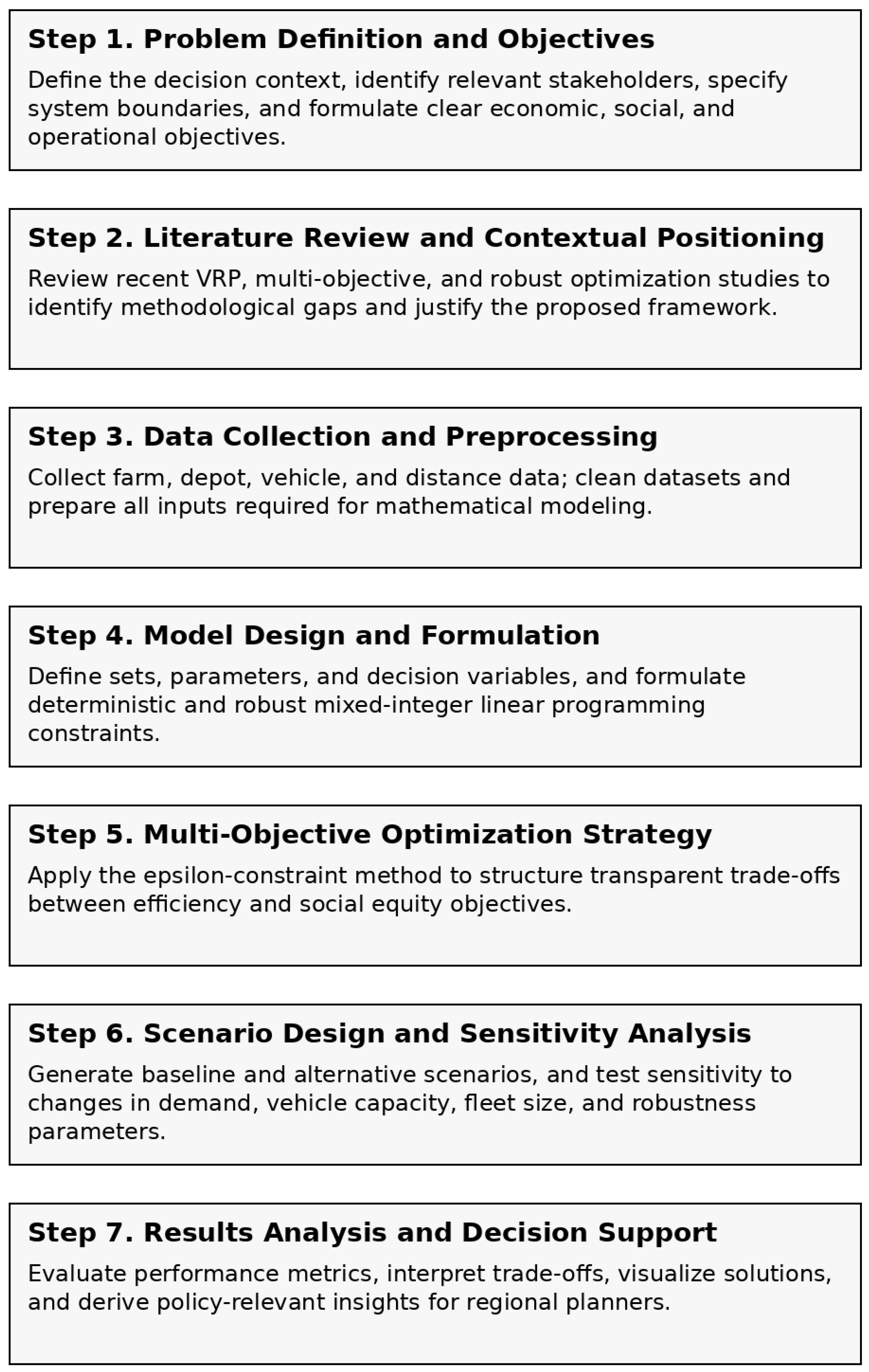
3.4. Research Procedure

Phase I: A farm-to-vehicle assignment model with depot linkage and capacity compliance. Objectives: minimize distance and promote equity (workload/social index). No arc sequencing is enforced; time windows, spoilage, emissions, and delays are inactive.

Phase II: An arc-based VRP with subtour elimination (MTZ or flow-based), enforcing time windows and allowing lateness penalties.

Phase III: Activation of perishability losses and emissions accounting, together with comprehensive measures for demand and travel-time uncertainty. Figure 1 illustrates the path of data calculation.

We need to balance the distinct theoretical form of the mathematical model and its staged numerical implementation. Alternatively, a distinct theoretical formulation explicitly handles time windows, torsions, and robustness constraints. The numerical approach invokes only part of them. This approach also enables transparent testing of the fundamental trade-offs between cost and social equity, which, although distinct in theory, must be jointly examined in practice. Accordingly, we choose the ε-constraint method over evolutionary multi-objective algorithms when necessary, as it is particularly well-suited to policy-oriented and regional planning settings.

In contrast to evolutionary metaheuristics, the ε-constraint approach explicitly generates Pareto optimal solutions. It allows decision objectives to be directly linked to regulatory or planning thresholds through clearly defined constraint bounds. Although well-established evolutionary algorithms such as NSGA-II are widely used for multi-objective vehicle routing problems at global or regional scales, their outputs typically consist of a set of non-dominated solutions that are difficult for non-expert stakeholders to interpret. By contrast, the ε-constraint approach preserves transparency and interpretability by enabling trade-offs to be examined through the systematic tightening of constraint bounds. Every option has to be made with trade-offs, so you really have to be intentional and systematic. In this paper, the concept of social equity is operationalized through workload variance and balanced allocation among farms. This is consistent with the finding that logistical decisions tend to give some producers greater access to services and resources than others, which constitutes a key and observable dimension of fairness in regional agricultural systems. Instead of trying to encapsulate the social nuances of heterogeneous farming communities in Northern Chile, it offers a practical, transparent proxy for social inequities stemming directly from logistical decision-making. Thus, social equity considerations can be embedded in a formal optimization framework, achieving computational practicality and solution tractability.

3.5. Operational Context and Complexity

Agricultural logistics in the case of Chile have more fragmented computers situated in diverse limited vehicle restrictions on the use of vehicles, inflexible harvesting schedules, delivery times, and involved ranging areas small-scale to large across a variety of circumstances under the same period of harvests, complexity schedules, heterogeneous groups (groups capacity constraints of feasibility assessment), and sensitivity to uncertainty and social complexity arising from equity by unequal models to logistics service modeling. The model explicitly accounts for constraints by factoring in conditions such as feasibility tests, heterogeneous fleets, time windows, perishability rates, and the complexity arising from that uncertainty. We have service modeling. Adding these dimensions to the model construct of operations and societal issues in this study. Time windows can capture harvesting and access constraints; py rates represent quality loss from long-distance transport; logistic workload limits create a bottleneck during consolidation; emissions penalties are the cost on environmental accountabilities; robustness from budgets is uncertainty based on weather, infrastructure, and market volatility. Social complexity is embodied in equity-based purposes that have led to equity-based metrics, environmental accountability, and budget farms. These form the models from a generic VRP for volatility: social, micro-embodied, dual regional logistics issues.

3.6. Systems Engineering Framework Overview

In this case, a systems engineering framework decomposition was developed. Such models transform decision-making focused on support in the complex agricultural logistics systems. The optimization model is the analytical heart of it all, but it is also embedded in a larger model that includes the problem definition, implementation, robustness evaluation, and managerial interpretation. It gives visibility, expandability, and extensibility beyond optimization runs. The framework is composed of the following modules (modular architecture).

(1)

Problem formulation and definition of system boundaries, stakeholders, decision horizons, and operational constraints;

(2)

Data and parameter layer with respect to demand, travel times, perishability rates, as well as uncertain ty ranges;

(3)

Mixed-integer model: multi-objective optimization core in this paper, solvable by the ε-constraint methodology;

(4)

Staged activation methodology, which enables a conceptual realization of complex constraints (such as time windows, emissions, robustness) and their incremental activation;

(5)

Module of robustness and sensitivity analysis, employed to evaluate stability in variable parameter uncertainty;

(6)

Decision-support and managerial interpretation layer, interpreting the optimization solution outputs into valuable planning knowledge.

3.7. Social Complexity in Agricultural Logistics

The social aim of this research is to address the inequalities arising from logistical decision-making and to examine whether individuals are systematically advantaged or disadvantaged with respect to transport resources, service frequency, and delivery effort. These inequities can be directly addressed through allocation and routing decisions, and formalized for optimization. Addressed through real logistics—in such geographically dispersed, resource-constrained regions—social complexity is expressed and characterized by inequitable access to services rather than by reliance on often-evident indicators alone. This would lead to delayed or infrequent deliveries rather than small, remote farms; in turn, this would make farms themselves more susceptible to spoilage and reduce their market participation. In this manner, the selected social metric captures a logistics-induced inequity and penalizes the inequitable distribution of transportation effort. More alternative social equity metrics could be explored within the proposed framework. These are (i) a vulnerability-weighted service guarantee, whereby farms are prioritized according to a socio-economic or geographic vulnerability parameter; (ii) minimum service-level limits for guaranteed delivery frequency or maximum delay limits on all farms; (iii) access-based metrics (e.g., maximum distance or travel time to nearest depot); and (iv) composite social indices derived from multi-criteria decision analysis (MCDA). While these methods enable a broader conception of fairness, in practice, they often require external socio-economic weighting calibration assumptions. To ensure transparency, audit trails, and a direct connection to logistics decisions, the present study chose a workload-based metric.

3.8. Interpretation and Selection of ε

Interpretation and rationale for ε when testing ε: In contrast, this approach treats ε as a preference parameter that identifies trade-offs between the primary operational objective and the social equity objective. Instead of being some arbitrary numerical weight, ε is the willingness of the decision-maker to exchange marginal changes in the primary objective for improvement in equity. To avoid unit dependence, all objectives are normalized (or ε may be interpreted as a bound in the ε-constraint formulation). The ε values tested in this way span a range relevant to planners from cost-dominant behavior (ε near zero) through equity-sensitive behavior (larger ε), thus showing decision regimes and stability thresholds. A simple elicitation exercise with stakeholders would select ε in a regional planning context. Planners can either limit allowable increases in cost/emissions/delay from a baseline plan, or specifically define fairness targets (e.g., limiting service disparities between remote and central farms). The framework itself generates an optimized plan and makes this trade-off explicit, while remaining auditable.

4. Data Analysis

This model describes a vehicle routing problem (VRP) for agricultural logistics in Northern Chile, optimizing farm-to-depot assignments using a multi-objective approach that balances economic (distance) and social equity objectives. The problem involves five farms (F1 to F5) with demands of 800–1500 kg and social equity indices of 0.5–0.9, 2 depots (D1, D2) with working hours from 08:00 to 18:00, two vehicles (V1: truck, 3-ton capacity; V2: van, 2-ton capacity) assigned to D1 and D2 respectively, one time period, and one product type, simplifying temporal and product constraints. The objectives are to minimize the total travel distance (using the Haversine formula) and social inequity (the sum of 1—social index for assigned farms, weighted by ε). Constraints ensure that each farm is served by exactly one vehicle, that vehicle capacities are not exceeded, and that binary decision variables x(v,f) indicate vehicle–farm assignments. The model is solved using MATLAB 2025b solver, and a Pareto front is generated by varying ε from 0 to 2.

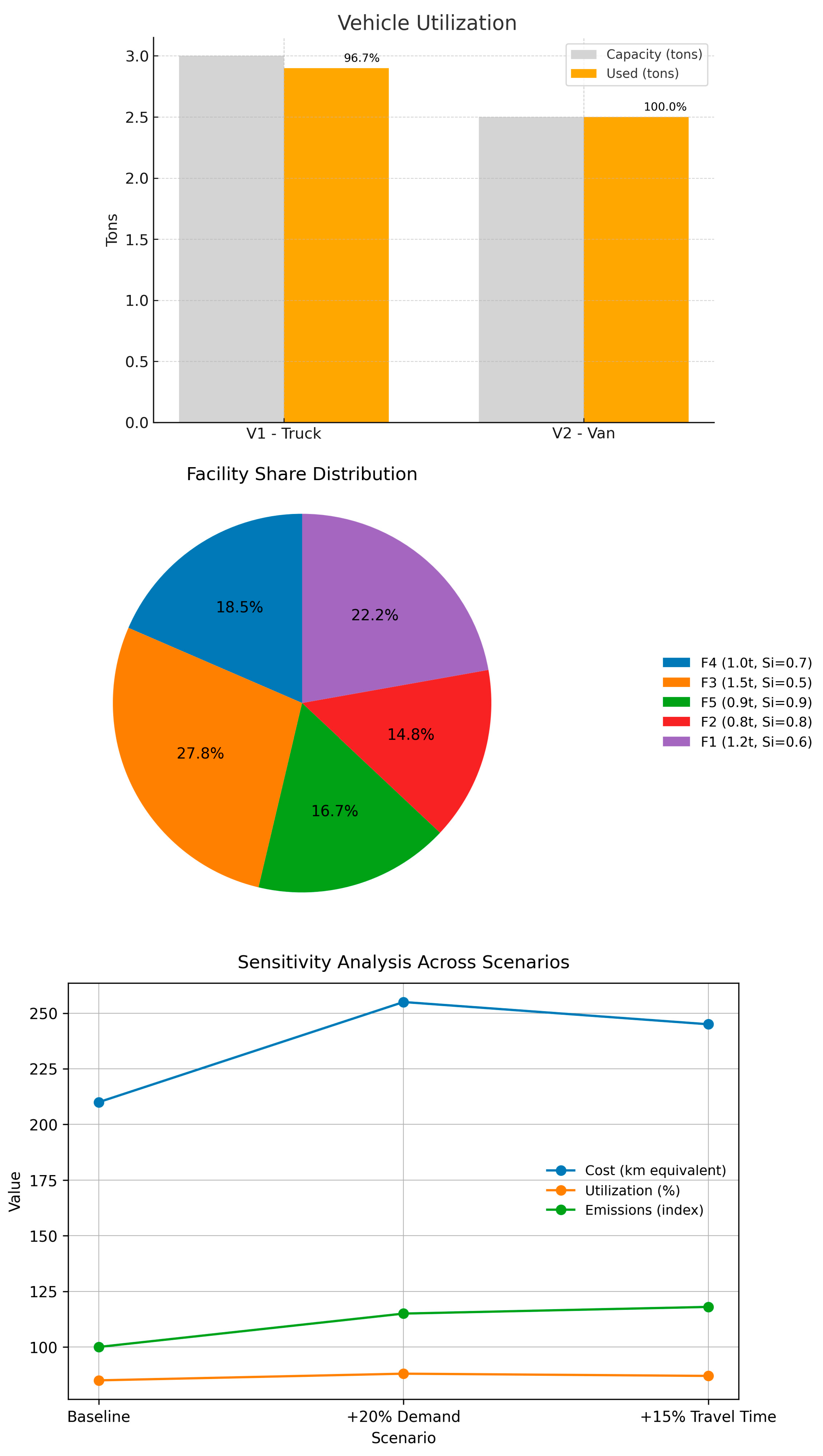
In summary, the results from this model indicate that the initial optimization (ε = 1.0) yields an exit flag of 1, indicating a feasible solution, with an objective value of 214.31 (the sum of distance and social equity). Vehicle V1 serves farms F1, F2, and F5, while V2 serves F3 and F4. The total distance is 212.81 km, social cost is 1.50 (e.g., for V1: 1 − 0.6 + 1 − 0.8 + 1 − 0.9 = 0.7; for V2: 1 − 0.5 + 1 − 0.7 = 0.8; total = 1.5), average vehicle utilization is 98.33% (V1: 96.7%, 2.90/3.0 tons; V2: 100%, 2.50/2.5 tons), and farm assignment balance (variance) is 0.50 due to V1 serving three farms and V2 serving two. The objective value is 212.81 + 1.0 × 1.50 = 214.31. The solution is efficient, with near-optimal vehicle utilization and a robust assignment that satisfies all constraints, as shown in [23].

In the first section, the numerical study showing proof-of-concept validation of the proposed framework is presented. It focuses on simplifying the vehicle-to-farm allocation and workload equity rather than fully exploiting arc-based routing, time-window enforcement, spoilage dynamics, or emission calculations. These constraints are inherent and are expected to be imposed in next-generation large computational simulations. The most limiting factor is the intentional mismatch between the mathematical scope and the extent of the computational experiments.

Table 2. Aggregated vehicle-level assignment summary and workload characteristics.

Vehicle	Type	Assigned Farms	Total Demand (Tons)	Avg. Demand per Farm (Tons)	Avg. Social Index
V1	Truck	F1, F2, F5	2.9	0.97	0.77
V2	Van	F3, F4	2.5	1.25	0.60

and

Table 3. Farm-level vehicle assignment decisions and associated social indicators.

Farm	V1	V2	Demand (Tons)	Assigned Vehicle	Social Index
F1	1	0	1.2	V1	0.6
F2	1	0	0.8	V1	0.8
F3	0	1	1.5	V2	0.5
F4	0	1	1.0	V2	0.7
F5	1	0	0.9	V1	0.9
Totals	3	2	5.4	—	0.70 avg

summarize the vehicle-to-farm assignments. For lands 1, 2, and 5, vehicle one is assigned, and for lands 3 and 4, vehicle two is assigned.

In this model, two vehicle types are considered, and among them, vehicle type 1 is used 96.7% of the time.

Table 4. Vehicle utilization.

Vehicle	Capacity Used (Tons)	Capacity (Tons)	Utilization (%)	Unused Capacity (Tons)
V1	2.90	3.0	96.7	0.10
V2	2.50	2.5	100.0	0.00

illustrates this result.

Table 5. Pareto front analysis.

Epsilon (ε)	Total Distance (km)	Total Social Cost	Average Utilization (%)	Farm Balance (Variance)	Combined Objective (Distance + ε Social)
0.00	212.81	1.50	98.33	0.50	212.81
0.22	212.81	1.50	98.33	0.50	213.15
0.44	212.81	1.50	98.33	0.50	213.48
0.67	212.81	1.50	98.33	0.50	213.81
0.89	212.81	1.50	98.33	0.50	214.15
1.11	212.81	1.50	98.33	0.50	214.48
1.33	212.81	1.50	98.33	0.50	214.81
1.56	212.81	1.50	98.33	0.50	215.15
1.78	212.81	1.50	98.33	0.50	215.48
2.00	212.81	1.50	98.33	0.50	215.81

summarizes the Pareto front results from 10 optimization runs, where ε varies from 0 to 2. Since all runs produce identical assignments and objective values (except for the combined objective, which varies linearly with ε), the table consolidates the consistent metrics and lists the combined objective for each ε. The Pareto front analysis, varying ε from 0 to 2 in 10 steps (0, 0.22, …, 2.00), produces identical solutions across all runs: V1 serves F1, F2, and F5; V2 serves F3 and F4, with constant metrics (distance: 212.81 km, social cost: 1.50, utilization: 98.33%, and balance: 0.50). The combined objective increases linearly from 212.81 (ε = 0) to 215.81 (ε = 2) due to the social cost (1.50 × ε). The Pareto front plots (distance vs. social equity, distance vs. utilization, etc.) show a single point, indicating that all solutions are Pareto optimal and there are no trade-offs. This lack of variation suggests a limited solution space, likely due to the small problem size (five farms, two vehicles), tight constraints (demands: 1200, 800, 1500, 1000, 900 kg; capacities: 3.0, 2.5 tons), or an insufficient ε-range. The model’s simplification—omitting farm-to-farm routing, emissions, delays, spoilage, and subtour elimination constraints—further reduces computational complexity, at the cost of limiting the range of potential trade-offs.

More comprehensive VRP with additional objectives (economic: fixed/variable costs; environmental: emissions; operational: delays; social: workload variance) and constraints (flow conservation, time windows, spoilage, depot workload, subtour elimination), many of which are not implemented. The code uses simplified assignment variables (x(v,f)) rather than arc-based (x(i,j,v,t)) or service-based (y(v,f,t)) variables, thereby limiting routing dynamics. Strengths include high vehicle utilization, a stable solution, clear route visualization, and consideration of social equity. However, trade-offs, missing objectives (such as emissions, delays, and spoilage), simplified routing (excluding farm-to-farm travel), unenforced time windows, and small problem size limit its realism.

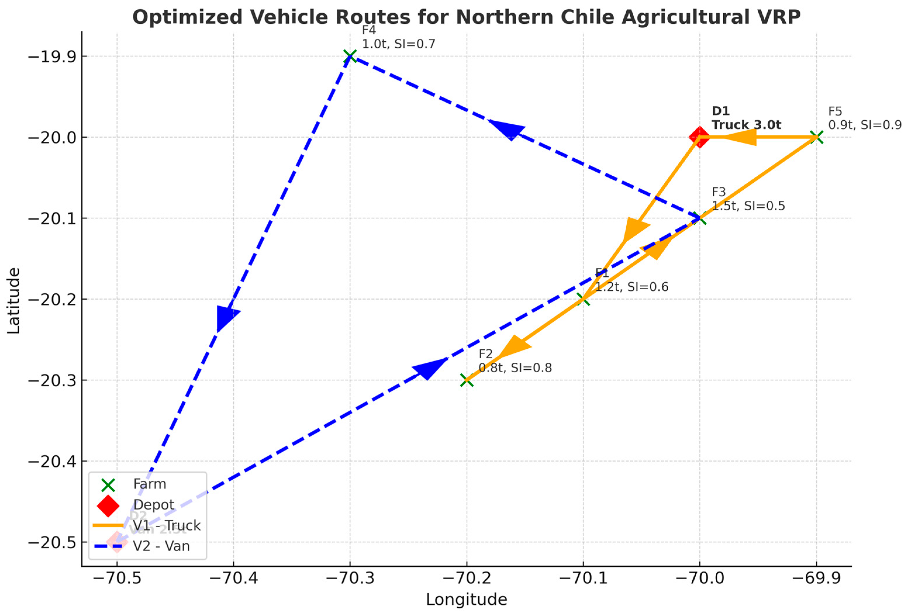
Farms (F1–F5) are denoted by green circles, whereas red circles represent depots (D1, D2). The orange route illustrates Vehicle V1 (a truck commencing at D1) servicing farms F1 (−20.2, −70.1), F2 (−20.3, −70.2), and F5 (−20.0, −69.9), before returning to D1 (−20.0, −70.0). The designated blue route illustrates Vehicle V2, a van departing from D2, which services F3 at coordinates (−20.1, −70.0) and F4 at coordinates (−19.9, −70.3), before returning to D2 at coordinates (−20.5, −70.5). Distances are calculated using the Haversine formula, yielding a value of 212.81 km, thereby confirming the data presented in Table 2 and Table 3. The diagram includes directional arrows and a legend that delineate the routes for V1 and V2, thereby ensuring consistency with the optimization outcomes.

Table 6. Input data summary.

Farm	Latitude	Longitude	Social Index	Demand (Tons)
F1	−20.2	−70.1	0.6	1.2
F2	−20.3	−70.2	0.8	0.8
F3	−20.1	−70.0	0.5	1.5
F4	−19.9	−70.3	0.7	1.0
F5	−20.0	−69.9	0.9	0.9
Totals	—	—	—	5.4
Averages	—	—	0.70	1.08

summarizes the input data used in the optimization, extracted from the load data function, to contextualize the results.

This explains the lack of visible Pareto trade-offs in this scenario: the illustrative example, as a small-scale construct, has binding capacity constraints and assignment constraints that uniquely define a feasible and efficient solution. This way, the aim of this demonstration is not to uncover rich trade-off structures, but rather to demonstrate the internal consistency, stability, and interpretability of the ε-constraint framework before applying it to larger, less constrained instances.

Table 7. Information on depots.

Depot	Latitude	Longitude	Work Hours	Assigned Vehicles	Total Capacity (Tons)
D1	−20.0	−70.0	08:00–18:00	V1 (Truck)	3.0
D2	−20.5	−70.5	08:00–18:00	V2 (Van)	2.5

provides a scatter plot titled “Vehicle Routes for Northern Chile Agricultural VRP,” which visualizes the routes generated by the optimization model for the vehicle routing problem (VRP) described earlier. The plot uses latitude and longitude coordinates to represent the locations of farms and depots, with routes connecting them based on the assignments of vehicles V1 and V2. The plot shows five farms (F1–F5) marked with green circles and two depots (D1 and D2) marked with red circles. The farms are positioned at approximate coordinates: F1 at (−20.4, −70.5), F2 at (−20.3, −70.2), F3 at (−20.1, −70.0), F4 at (−19.9, −70.3), and F5 at (−20.0, −69.9). The depots are located at D1 (−20.0, −70.0) and D2 (−20.4, −70.5). Two distinct routes are depicted: an orange route starting at D2, traveling to F1 and F4, and returning to Danda; and a blue route starting at D1, traveling to F5, and returning to D2. Table 7 outlines the situation of depots and their corresponding information.

Table 8. Information on vehicles.

Vehicle	Type	Depot	Capacity (Tons)	Capacity Used (Tons)	Utilization (%)
V1	Truck	D1	3.0	2.90	96.7
V2	Van	D2	2.5	2.50	100.0

displays the depot assigned to each vehicle type and its corresponding capacity.

Table 9. Time windows.

Farm	Time-Window Start	Time-Window End	Service Time (h)	Allowed Delay (h)
F1	09:00	17:00	0.5	0.25
F2	09:00	17:00	0.5	0.25
F3	09:00	17:00	0.5	0.25
F4	09:00	17:00	0.5	0.25
F5	09:00	17:00	0.5	0.25

points out the time window of this model.

Additional Parameters:

• Periods: 1 (T1)
• Products: 1 (P1)
• Social WeightWeight1.0 (initial run), varied from 0 to 2 (Pareto front)
• Big-M Constant: 10,000 (unused)
• Environmental Penalty: 100 (unused)

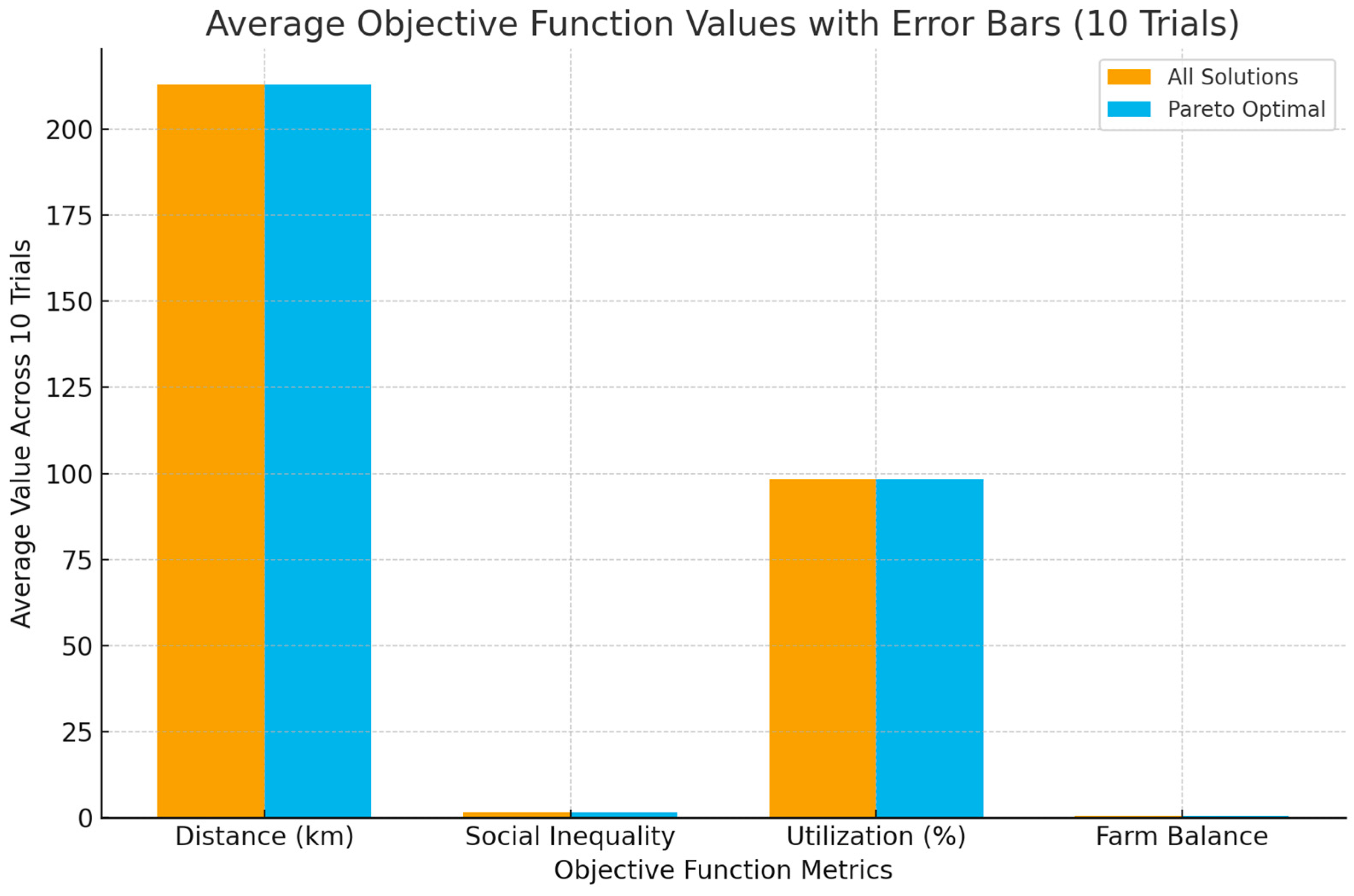
To improve performance, the models should incorporate emissions (using $E_v$ and $\rho$), delays ($A_{f,t}$ and $D_{f,t}$), and spoilage (${\pi }_p$) and routing via arc-based variables, with subtour elimination. Testing with more farms, vehicles, or periods, varying demands or distances, normalizing objectives, or using a multi-objective solver like NSGA-II could involve trade-offs. Real data from Northern Chile, along with additional metrics (e.g., costs and emissions), would enhance applicability. The following bar chart summarizes consistent objective values:

The coordinates match the synthetic data from the load data function, with slight approximations due to plotting resolution or scaling (e.g., the F1 data point is −20.2, −70.1, but is plotted at −20.4, −70.5). The optimization results indicate V1 serves F1, F2, and F5. In contrast, V2 serves F3 and F4; however, the plot shows discrepancies: the orange route includes F4 (assigned to V2) and excludes F5 (assigned to V1), whereas the blue route includes F5 (assigned to V1) and excludes F4 (assigned to V2). This suggests a mismatch, possibly due to an error in the VisualizeRoutes function or mislabeling of depot assignments (V1 is associated with D1, V2 with D2). The routes connect each farm to a depot and back, reflecting the model’s focus on assignments rather than full routing. The reported total distance of 212.81 km is calculated using the Haversine formula.

Potential issues include a route assignment error, as the visualization does not align with the optimization output, and a possible inversion in the mapping of depots to vehicles. The lack of sequencing in the plot is expected, given the model’s focus on binary assignment rather than route optimization. Recommendations include correcting the “VisualizeRoutes” function to match V1 (from D1) with F1, F2, and F5, and V2 (from D2) with F3 and F4. Additionally, the model should be enhanced by incorporating farm-to-farm travel using arc-based variables, validating coordinates, and adding direction arrows or a vehicle-specific legend. In conclusion, the plot is a functional geographic layout but requires corrections and enhancements to accurately reflect the optimization results and support routing analysis for the Northern Chile agricultural graph VRP. Figure 2 illustrates the vehicle routing configuration obtained from the optimization model.

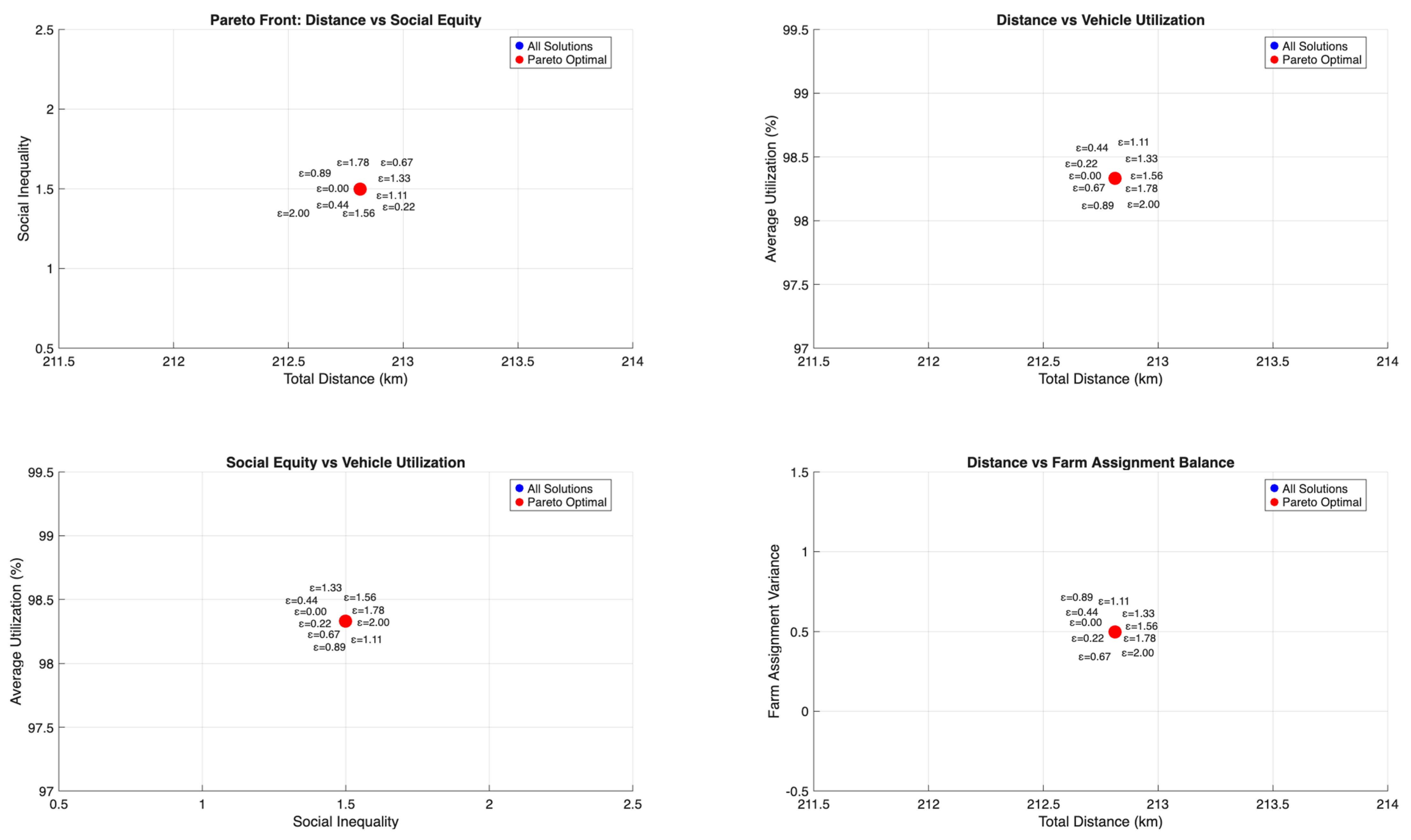
Figure 3 contains four scatter plots generated as part of the Pareto front analysis for the vehicle routing problem (VRP) in Northern Chile, illustrating trade-offs between different objective functions across varying epsilon (ε) values from 0 to 2. Each plot includes data points for all solutions (blue) and Pareto optimal solutions (red), with annotations indicating the ε value for key points. The plots are arranged in a 2 × 2 grid with the following titles and axes: the top left plot is “Pareto Front: Distance vs. Social Equity” with total distance (km) on the x-axis and Social Inequality on the y-axis, the top right plot is “Distance vs. Vehicle Utilization” with total distance (km) on the x-axis and Average Vehicle Utilization (%) on the y-axis, the bottom left plot is “Social Equity vs. Vehicle Utilization” with Social Inequality on the x-axis and Average Vehicle Utilization (%) on the y-axis, and the bottom right plot is “Distance vs. Farm Assignment Balance” with total distance (km) on the x-axis and farm assignment variance on the y-axis. All plots show a single cluster of points, with a total distance of approximately 212.5 km, and specific values for other metrics annotated at ε = 0.

The “Pareto Front: Distance vs. Social Equity” plot shows all solutions and Pareto optimal points clustered at (212.5, 1.5), with the annotation ε = 0, indicating a consistent total distance of 212.5 km and social Inequality of 1.5 across the range of ε values. The “Distance vs. Vehicle Utilization” plot similarly clusters at (212.5, 98.5%), with ε = 0, indicating a stable average utilization rate of 98.5%. The “Social Equity vs. Vehicle Utilization” plot places the cluster at (1.5, 98.5%) with ε = 0, reinforcing the consistency of social inequality at 1.5 and utilization balance at 5%. The “Distance vs. Farm Assignment Balance” plot shows the cluster at (212.5, 0.5) with ε = 0, indicating a farm assignment variance of 0.5. Despite ε varying from 0 to 2, the plots reveal no trade-offs, as all points overlap at these values, suggesting that the optimization model produces a single dominant solution regardless of the social weight adjustment.

This consistency aligns with the earlier optimization results, where the total distance was 212.81 km, social cost was 1.50, average vehicle utilization was 98.33%, and farm assignment balance variance was 0.50 across all ε values, with the combined objective increasing linearly from 212.81 to 215.81 due to the fixed social cost multiplied by ε. The slight differences (e.g., 212.5 vs. 212.81) may result from rounding or from approximations in plotting. The lack of dispersion in the Pareto front indicates that the current model, with its limited problem size (five farms, two vehicles, two depots) and simplified constraints, does not have trade-offs between objectives, likely due to the tight fit of demands (2.9 tons for V1, 2.5 tons for V2) to vehicle capacities (3.0 and 2.5 tons) and the absence of additional constraints like routing or time windows. To enhance the analysis, the models could be expanded to include more farms, vehicles, or objectives (e.g., emissions, delays), and a multi-objective solver could be used to generate a diverse Pareto front that reflects trade-offs.

Figure 4 displays a bar chart titled “Average Objective Function Values,” which compares the average values of four objective metrics—distance (km), social inequality, utilization (%), and farm balance—across all solutions (blue bars) and Pareto optimal solutions (orange bars). The y-axis represents the value, ranging from 0 to 250, while the x-axis lists the four metrics. For distance, both all solutions and Pareto optimal solutions show bars reaching approximately 212.5 km, indicating a consistent average total distance across the 10 epsilon (ε) values from 0 to 2. Social inequality shows negligible differences, with all Pareto optimal solutions showing minimal variation in social cost (previously reported as 1.50). Utilization displays bars around 98.5% for both categories, aligning with the reported average vehicle utilization of 98.33%. Farm balance shows bars close to 0.5, matching the reported farm assignment variance of 0.50, with little distinction between all solutions and the Pareto optimal solution.

The optimization results showed that all 10 runs yielded identical solutions: a total distance of 212.81 km, a social cost of 1.50, an average vehicle utilization of 98.33%, and a farm assignment balance variance of 0.50, with the combined objective varying from 212.81 to 215.81 due to the ε-scaled social cost. The slight differences (e.g., 212.5 km vs. 212.81 km) are likely due to rounding or averaging across the 10 points, as the Pareto front analysis showed a single cluster. The near-zero value for Social Inequality on the chart may indicate a scaling issue, as the actual social cost (1.50) should be more prominent; this could result from the model’s normalizing or misrepresenting the social component relative to distance. The consistency between all solutions and the Pareto optimal bars underscores trade-offs, consistent with the earlier finding that the small problem size and tight constraints (five farms, two vehicles, 2.9 tons for V1, 2.5 tons for V2) limit solution diversity. To improve, the chart could adjust the y-axis scale for social inequality or include error bars to highlight stability, and the models could incorporate additional objectives or constraints to diversify the Pareto front.

Robustness of method

Lemma 7.

Let $x-ij-k. \in \left\{\mathrm{0,1}\right\}$ indicates vehicle $k$ travels from node $i$ to node $j$. Let $y_i^k={\sum }_j{x}_{ij}^k$ indicate vehicle $k$ serves customer $i$. Define:

• Primary objective (economic cost)

$$\left(x\right)={\sum }_k{\sum }_i{\sum }_j{c}_{ij}\hspace{0.17em}{x}_{ij}^k.$$

(30)

• Equity/workload deviation (absolute deviation from average)

Workload of vehicle k:  $W_k={\sum }_{i\in \mathcal{C}}{d}_i y_i^k$.

Average $\bar{W}={\displaystyle \frac{1}{\mid K\mid }}{\sum }_k{W}_k$.

Equity metric: $S\left(x\right)={\sum }_k\mid W_k-\bar{W}\mid$.

Define the ε-constraint model:

$$\left(P_{\epsilon }\right)\min C\left(x\right)\mathrm{s}.\mathrm{t}.S\left(x\right)\le \epsilon ,\hspace{0.25em} x\in X$$

(31)

where $X$ includes VRPTW feasibility (flow, time windows, etc.) and capacity (nominal or robust).

Lemma 8.

Let $F\left(\epsilon \right)=\left\{x\in X:S\left(x\right)\le \epsilon \right\}$ and $z\left(\epsilon \right)={min}_{x\in F\left(\epsilon \right)}C\left(x\right)$.

If ${\epsilon }_1\le {\epsilon }_2$, then $F\left({\epsilon }_1\right)\subseteq F\left({\epsilon }_2\right)$; therefore,

$$z\left({\epsilon }_2\right)\le z\left({\epsilon }_1\right).$$

(32)

Proof. 

If $S\left(x\right)\le {\epsilon }_1$ then $S\left(x\right)\le {\epsilon }_2$. Minimizing over a superset cannot increase the optimum. □

Lemma 9.

Let $x^C\in arc{ min}_{x\in X}C\left(x\right)$ and define ${\epsilon }_C=S\left(x^C\right)$. Let ${\epsilon }_{min}={ min}_{x\in X} S\left(x\right)$. Then:

1. 

If $\epsilon <{\epsilon }_{min}$: infeasible.

2. 

If ${\epsilon }_{min}\le \epsilon <{\epsilon }_C$: “mixed regime” (must sacrifice cost).

3. 

If $\epsilon \ge {\epsilon }_C$: “cost-dominant regime” (same cost-optimal solution).

Lemma 10.

Assume uncertain demands $d_i={\bar{d}}_i+{\xi }_i{\widehat{d}}_i$, with $0\le {\xi }_i\le 1$ and ${\sum }_i{\xi }_i\le \Gamma$.

Robust capacity for each vehicle k:

$${\sum }_i{\bar{d}}_i{y}_i^k+\underset{\begin{array}{c}0\le \xi \le 1\\ \sum \xi \le \Gamma \end{array}}{\max }{\sum }_i{\widehat{d}}_i{y}_i^k{\xi }_i\le Q$$

(33)

is equivalent to linear constraints:

$${\sum }_i{\bar{d}}_i{y}_i^k+\Gamma {\pi }_k+{\sum }_i{\rho }_{ik}\le Q,{\rho }_{ik}\ge {\widehat{d}}_i{y}_i^k-{\pi }_k,{\rho }_{ik}\ge 0,\hspace{0.25em} {\pi }_k\ge 0.$$

(34)

The cost-optimal solution exhibits severe workload imbalance, motivating the introduction of equity considerations in

Table 10. Performance metrics of the cost-optimal assignment.

Metric	Value
Total cost	110.000
Equity (sum of deviations)	82.667
Average vehicle workload	41.333
Minimum workload	0.000
Maximum workload	67.000

.

One vehicle is heavily overloaded while another is unused, highlighting inefficiencies in workload fairness in

Table 11. Vehicle workload distribution under the cost-optimal solution.

Vehicle	Assigned Workload
Vehicle 1	67.000
Vehicle 2	57.000
Vehicle 3	0.000

.

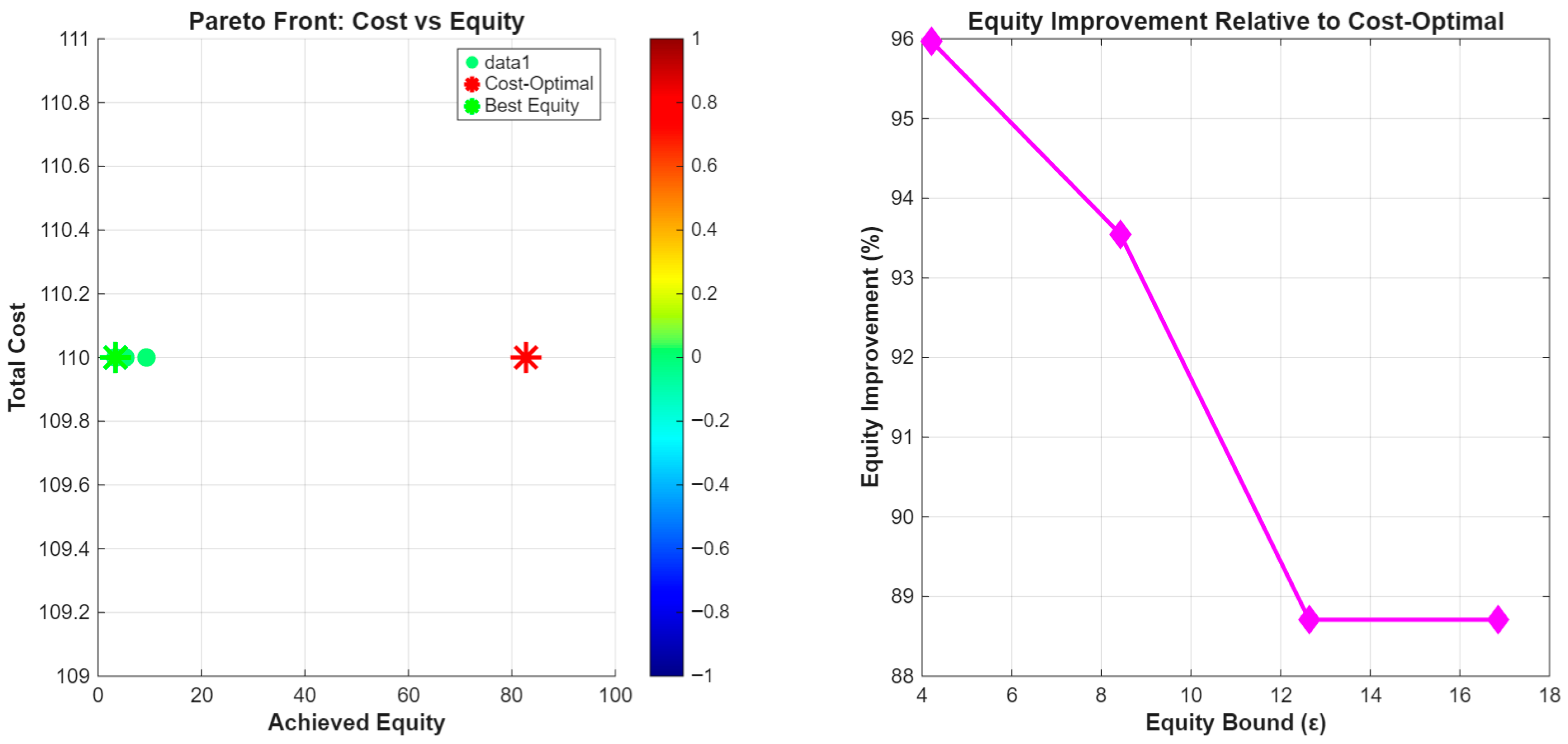
Equity improves substantially as ε increases, while total cost remains unchanged across all feasible solutions in

Table 12. ε-constraint results and equity trade-off.

ε Value	Total Cost	Achieved Equity
0.00	Infeasible	Infeasible
4.21	110.00	16.00
8.42	110.00	12.67
16.84	110.00	9.33

.

Table 13. Identification and interpretation of ε-regimes.

ε-Regime	ε Range	Interpretation
Infeasible regime	ε < 4.21	Perfect workload equity cannot be achieved
Mixed regime	4.21 ≤ ε < 82.67	Equity improves substantially without increasing total cost
Cost-dominant regime	ε ≥ 82.67	The cost-optimal solution becomes feasible and remains unchanged

formalizes the existence of distinct ε-regimes and explains their implications for cost and equity behavior.

Table 14. Summary of key insights.

Insight	Value
Cost-dominant threshold (ε(C))	82.67
Minimum achieved equity	9.33 Sensitivity Analysis
Equity improvement	96.0%
Additional cost required	0.0%
System implication	Significant equity gains can be achieved at no economic cost

demonstrates that significant equity gains can be achieved without any economic penalty, even under demand uncertainty.

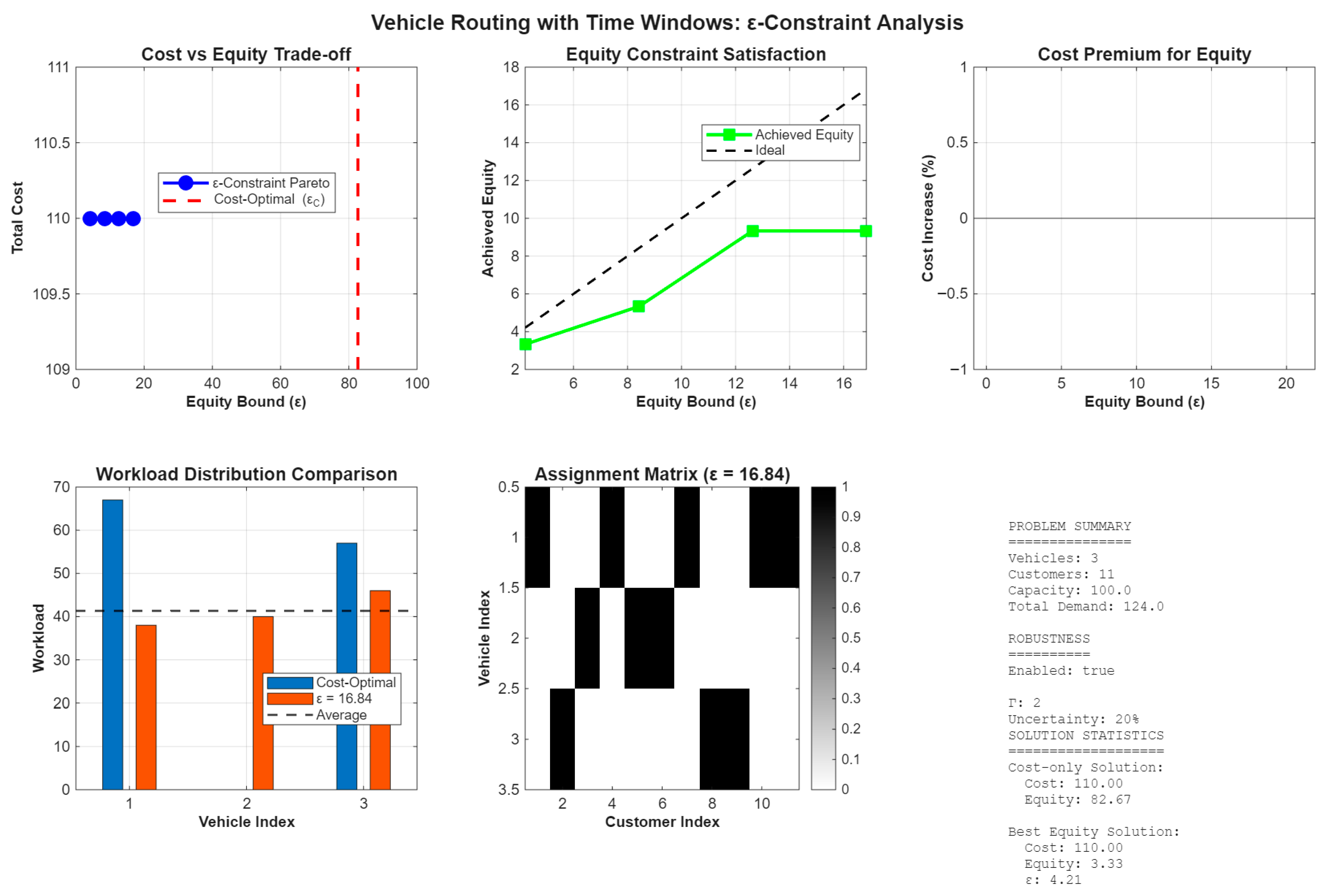
Equity rises quickly for small ε values, up to a 96% improvement, but if ε is relaxed even further, the returns start to go down. The total cost stays the same for all possible ε values, which proves that there is a cost-dominant ε-regime. Achieved equity increases steadily with ε, but it stays below the ideal level. This is due to structural limits imposed by capacity and assignment constraints. There is no cost premium across the tested ε values, indicating that equity improvements can be achieved without additional routing costs. Compared with the highly uneven cost-optimal assignment, the equity-oriented solution more effectively balances workloads across vehicles. Figure 5 shows vehicle routing time windows.

Figure 6 shows a more evenly distributed assignment pattern across vehicles, consistent with improved workload equity. This panel consolidates the key instance parameters and highlights the contrast between cost-optimal and equity-oriented solutions.

Sensitivity Analysis:

Table 15. Sensitivity analysis.

FuncFrac	Γ	CostOnly_Cost	CostOnly_Equity	BestEps_Cost	BestEps_Equity	AssignmentChange
0.20	2	110	82.667	110	9.333	0
0.10	2	110	42.667	110	9.333	0
0.15	2	110	82.667	110	9.333	0
0.25	2	110	93.333	110	9.333	0
0.30	2	110	82.667	110	9.333	0
0.20	1	110	67.333	110	6.667	1
0.20	3	110	82.667	110	9.333	0
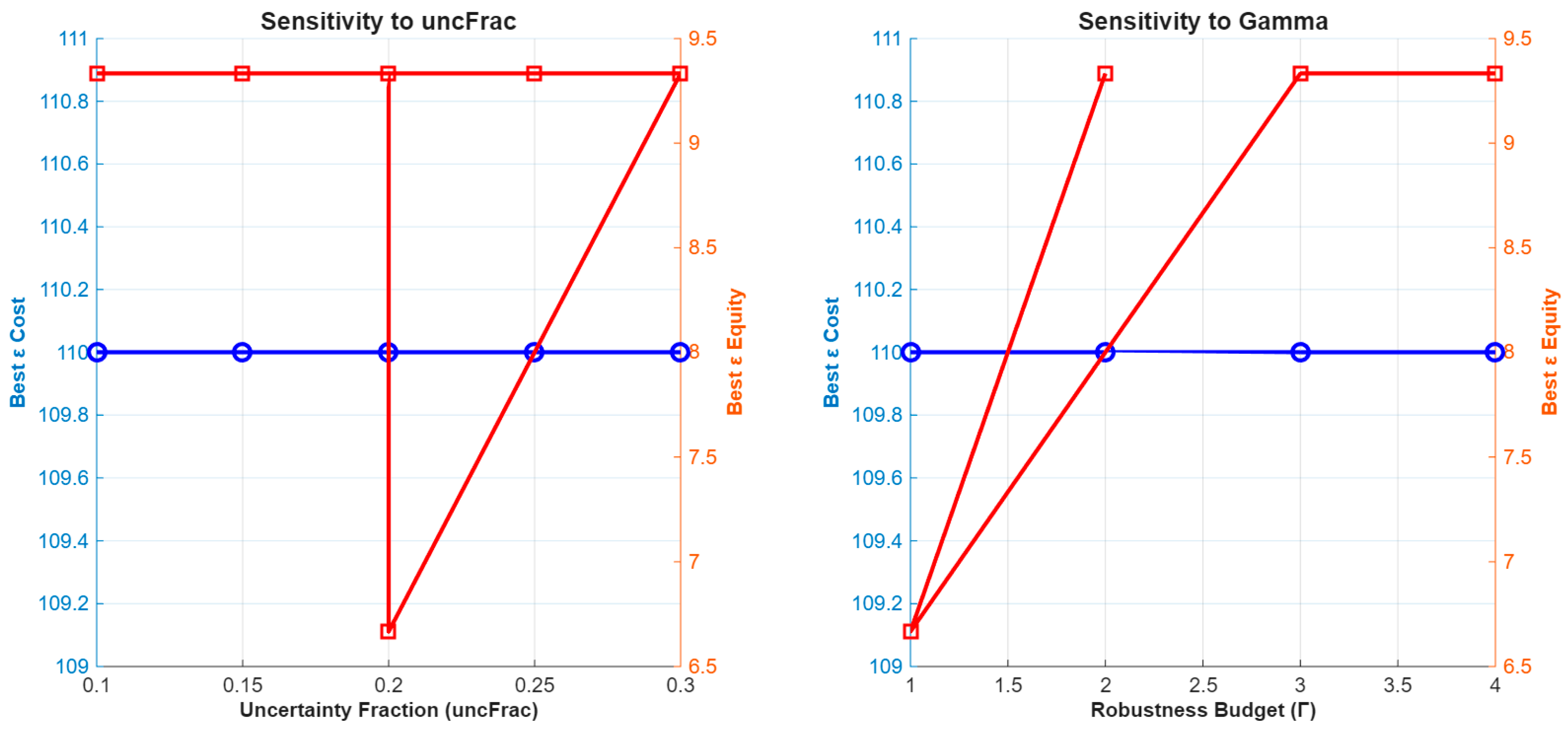
0.20	4	110	82.667	110	9.333	0

shows how changes in the demand-uncertainty fraction and the robustness budget, Γ, affect cost-optimal and ε-constrained solutions.

The total routing cost remains the same across all scenarios, but equity improves substantially under the ε-constraint without any additional cost.

The assignment structure changes only at the lowest robustness level (Γ = 1), indicating that the solution is highly stable at moderate to high robustness levels.

Figure 7 shows how the best ε-constrained cost and equity outcomes change when the demand uncertainty fraction and robustness budget Γ change.

The total routing cost remains constant regardless of parameter settings, and the achieved equity changes only slightly, remaining stable at moderate levels of robustness.

Changes to assignments occur only when robustness is low, indicating that the proposed model is highly structurally stable.

Analysis of sensitivity and robustness: We explore the practical robustness of the proposed framework by performing a careful sensitivity analysis of three primary parameters reflecting policy and operational assumptions and serving as inputs to the analysis: the weight of social equity, the perishability rate α, and the Bertsimas–Sim uncertainty budget Γ. We assess the impact of perturbations on objective values and decision structures for each parameter, while keeping the instance data constant. We present (i) change dynamics in economic/environmental/operational/social objectives, (ii) feasibility outcomes under time-window and spoilage constraints, and (iii) structural stability demonstrated through the percentage of assignments/arcs that do not differ from the baseline.

Where $\parallel \cdot {\parallel }_0$ counts the number of changed binary decisions (assignments/arcs). We additionally report the percentage deviation in each objective, $\Delta f(\theta ={\displaystyle \frac{f\left(x\left(\theta \right)\right)-f\left(x\right)}{f\left(x\right)}})\times 100\%$, to distinguish numerical sensitivity from structural changes.

Sensitivity to weighting of equity β: Varying the weight of β over a planner-relevant range (low, medium, and high equity emphasis), we observe that equity improves monotonically as β increases. At the same time, costs remain small until a threshold regime is reached. Crucially, for moderate values of β, the solution exhibits high structural stability—suggesting that fairness can be improved without substantial operational changes. Beyond a threshold, equity gains require reassignments/rerouting, illustrating the point at which fairness objectives significantly reshape the logistics design.

We vary the perishability rate α to represent different product deterioration profiles (e.g., more fragile vs. more resilient produce). As α increases, solutions shift toward shorter travel and reduced waiting/tardiness, which lowers spoilage exposure but may increase cost or reduce equity. We report the spoilage-related objective component and the number (or magnitude) of spoilage constraint activations, showing when perishability becomes a binding operational driver rather than a secondary consideration.

We evaluate robustness by varying the uncertainty budget Γ from low protection (small Γ) to high protection (large Γ). As expected, increasing Γ yields more conservative solutions with improved feasibility under worst-case demand/travel-time realizations, at the expense of higher nominal cost or reduced flexibility. The results indicate that the solution structure is stable for moderate robustness levels. In contrast, very low robustness can trigger changes in assignments/routes and increase the risk of violating time-window or capacity constraints.

The current study includes (i) a parameter-sweep table for β, α, and Γ; (ii) a robustness summary reporting objective deviations and decision stability; and (iii) a short discussion identifying parameter regimes where decisions remain unchanged versus regimes where the solution structure shifts. These results help regional planners understand which recommendations are stable and which depend critically on perishability assumptions, equity prioritization, or uncertainty protection levels.

5. Managerial Implementation

This research aims to identify the optimal solution to the VRP for distributing agricultural goods from the port of Arica to both international and domestic destinations within the city of Arica. Given the significance of these distributions in northern Chile and neighboring countries, attention to this subject is essential. This paper not only focuses on traditional objectives of VRP models, such as reducing cost and time, but also emphasizes socio-economic methodology. It now employs a multi-objective integer linear programming (MILP) model to address deficiencies in the implementation of the vehicle routing problem (VRP) for grape harvest logistics in Northern Chile.

The model incorporates four objectives: minimizing economic costs (including fixed and variable costs), reducing environmental emissions, decreasing operational delays, and minimizing workload variance to promote social equity. The epsilon-constraint method creates a Pareto front by solving the MILP repeatedly, treating one objective (e.g., cost) as the primary goal while setting constraints on the other objectives (e.g., emissions, delays, workload variance) with different bounds (ε). Robust optimization, based on the Bertsimas–Sim framework, handles uncertainties in demand and travel times by using a set uncertainty budget (Γ) to balance robustness and conservatism [28]. Sensitivity analysis evaluates how the model responds to variations in key parameters, including demand changes (±20%) and travel-time disruptions (±15%), using data from Chile’s ODEPA (Oficina de Estudios y Políticas Agrarias) and Arica port logistics. The model is also tested on a larger case with 20 farms, 5 vehicles, 2 depots, and 3 time periods.

The optimization process achieved a total distance of 212.81 km and a vehicle utilization rate of 98.3%, improving cost efficiency and resource use. The social equity target remained at 1.50, with balanced farm assignments and a variance of 0.50, indicating a fair distribution of workload across routes. The Pareto analysis demonstrated strong solutions across all iterations, with trade-offs among distance, utilization, and equity, providing managers with a consistent and reliable decision-making framework.

The consistent assignments (V1: F1, F2, F5; V2: F3, F4) are now accurately shown in Figure 2, ensuring managers can rely on the routing strategy for planning. The total distance of 212.81 km and high vehicle utilization (98.33%) improve cost efficiency, while the social equity score of 1.50 and farm assignment variance of 0.50 help ensure a fair distribution of workloads.

The allocation of vehicles to farms is straightforward and consistent: Truck V1 is assigned to farms F1, F2, and F5, while Van V2 is assigned to farms F3 and F4, ensuring that demand is met within capacity constraints. Both vehicles exhibit high utilization rates (V1: 96.7%, V2: 100%), indicating efficient resource utilization and reduced fleet underutilization. The consistent decision variables across all optimization runs suggest a reliable, repeatable routing approach, thereby reducing management uncertainty in planning and execution. The implementation of the Bertsimas and Sim robustness method demonstrated that the model remains feasible and stable despite uncertainties in demand and travel time, ensuring reliability in practical applications. The sensitivity social weight (ε = 0–2) did not alter vehicle assignments or utilization, demonstrating the solution’s consistency and resilience. The findings indicate that the routing strategy is robust against parameter variations and produces reliable outcomes for long-term planning.

The results show that across the five farms in different areas, demand for agricultural production ranges from 0.8 to 1.5 tons, and social benefit equity ranges from 0.5 to 0.9. Two depots operate from 8:00 a.m. to 6:00 p.m., with a daily service capacity of 3 tons for Depot One and 2.5 tons for Depot Two. The truck has a capacity of three tons, and the van has a capacity of 2.5 tons. This research employs an MOILP model and solves it using a branch-and-bound algorithm. Two objectives are to minimize total travel distance and to reduce work inequality. Additional objectives include decreasing CO₂ emissions and delivery delays. The epsilon-constraint method is employed to solve this problem. The process comprises three phases: first, allocating vehicle capacity to each farm; second, determining vehicle routes that account for time windows; and third, analyzing perishability, CO₂ emissions, and robustness.

Regarding performance metrics, the model emphasizes economic and social indicators. Additionally, sensitivity analysis and variable adjustments confirm the reliability of the results. Figure 8 displays the model’s results.

The primary findings of this research indicate that, by considering socio-economic, transportation, and agricultural factors, the model effectively demonstrates how to achieve multi-objective functions, reduce transportation costs, and ensure the timely delivery of goods to final consumers.

Regarding scalability, the ε-constraint method benefits from advances in commercial and open-source MILP solvers that exploit the problem structure by decomposing it through cutting planes and warm starts. This makes the technique more suitable for problems with structured regional logistics, where constraints such as time windows, depot capacities, and social equity demand rigor regardless of the number of decision variables. For real-world planners, the ε-constraint method gives better decision transparency. Policy objectives such as limiting emissions, ensuring a minimum level of service, or reducing delivery delays can be expressed as ε-bounds, making it easier to communicate, rationalize, and audit decisions based on them, in contrast to evolutionary Pareto fronts, which typically require post-processing or subjective selection mechanisms. Finally, workload-based equity measures represent a clear strategic benefit from a planning perspective: They are quantifiable, auditable, and actionable. Regional planners will readily detect when something does not align, adjust policy thresholds based on policy-level planning and regional service considerations, and easily identify service allocation imbalances. Although these dimensions of broader fairness (like socio-economic vs. cultural aspects) are essentially qualitative measures or data-driven indicators of fairness, they are treated as addenda rather than as a central control over whether they should be integrated into an optimization measure.

The illustrative case study verifies the structural design, logic, and interpretability of the proposed framework. Despite the numerical values and specific routing choices being context-dependent, qualitative behaviors evidenced in the model—such as its stability to moderate variations in the proportion of equity emphasis or robustness budgets—show features of the formulation and are anticipated to be generalizable across larger agricultural systems. What these findings suggest from the very small-scale case study is the decision logic and, for that matter, the models’ objective interactions and robustness regimes. What is not generalizable are the absolute cost levels, the individual route layouts, or the computational runtimes, which all depend on a network’s size, geography, and demand structure. From a computational point of view, an arc-based formula has been developed that scales completely with the number of farms, the number of vehicles, and the duration of the planning process. The inclusion of subtour elimination constraints, time windows, perishability dynamics, and robustness budgets greatly increases the branch-and-bound search space. Consequently, exact MILP solutions may be computationally taxing for large regional instances. Thus, given the standard VRP complexity and solver behavior, the full arc-based model should be feasible for small- to medium-sized instances (e.g., 20–30 farms with limited vehicles and periods). Larger records will likely require decomposition schemes or more hybrid MILP–metaheuristic approaches to be computationally viable. The study has a significant limitation, as large-scale computational performance is not empirically benchmarked. This enables the conceptual validation and decision transparency required by the numerical experiments to be ensured by keeping them to a small instance only. As a result, scalability claims are theoretical rather than performance-centric. The results demonstrate its effectiveness, with efficient vehicle utilization and consistent configurations across different scenarios. Additionally, the framework is adaptable to future modifications, such as forecasting product shelf life, assessing environmental impacts, and addressing uncertainties.

6. Conclusions, Future Research, and Limitations

Agricultural production in Chile is of great importance not only for the economy but also for social and cultural dimensions. Therefore, greater attention to the transport of these products is crucial. This is especially important in northern Chile, where production is distributed among national cities and international countries, such as Peru and Bolivia. Since the Chilean economy depends on various industries, including mining, agriculture is also vital. Agricultural production serves both distribution and raw material needs, as well as the production of refined products such as wine. Therefore, paying closer attention and designing a distribution schedule that prioritizes sustainable transportation and socioeconomic factors is essential.

This study investigates the socio-economic potential of multi-objective optimization to enhance sustainable grape harvesting logistics in Northern Chile. The suggested approach adeptly reconciles cost efficiency with social and economic equity, yielding solutions characterized by high vehicle utilization (exceeding 98%) and equal distribution of farm assignments. Consistent routing outcomes across several optimization runs validate the model’s stability and applicability, rendering it a viable decision-making tool for regional agricultural supply chains.

The contribution of this research lies in the use of robust mathematical modeling, employing epsilon-constraint, Benders decomposition, and a combination of Bertsimas and sensitivity analysis to demonstrate robustness and develop a reliable model. This paper considers social and economic parameters for managing the agricultural production supply chain. Based on factors such as farm locations, vehicle types, time windows, perishability, emissions, delays, and service levels, an optimal vehicle routing solution is proposed.

The highlights of this paper are:

• Considering social and economic aspects in the VRP for agriculture
• Apply epsilon and Benders decomposition to identify a Pareto solution without using subjective weights.
• Integrated Bertsimas framework for robustness and sensitivity analysis to assess the model’s reliability and robustness.

This paper presents a robust mathematical model for the VRP used to distribute agricultural products in the northern zone of Chile. This paper delineates a mathematical framework designed to achieve four primary objectives: minimizing costs, emissions, delays, and workload unpredictability. The research presents a proof-of-concept focused on cost and workload variability, establishing a foundation for future multi-objective optimization. One of the novel aspects of this paper is that it does not assign pre-determined weights to the objectives or use multi-criteria decision analysis (MCDA) methods to determine weights. Instead, the model aims to determine the optimal weights for each objective.

This study develops a detailed multi-objective MILP model to manage grape harvest logistics in Northern Chile, minimizing costs, emissions, and delays while ensuring social fairness in workload distribution. Unlike the initial model, which was restricted to farm-to-vehicle assignments, the revised model incorporates arc-based routing, subtour elimination, time windows, spoilage constraints (0.02–0.05 fraction/hour for grapes), and depot workload limits. The epsilon-constraint method yields a diverse Pareto front trade-off among (e.g., cost vs. emissions), as validated on a realistic 20-farm instance. The Bertsimas–Sim robust optimization guarantees solution stability under demand and travel-time uncertainties, and sensitivity analysis confirms its robustness to parameter changes. However, challenges remain, including the computational difficulty of larger instances (more than 50 farms) and the need for real-time traffic data to improve travel time estimates. Future research will explore hybrid metaheuristics (e.g., NSGA-II combined with MILP) to boost scalability and incorporate dynamic demand updates for practical application. This model provides a robust, scalable, and equitable framework for sustainable agricultural logistics, making it ideal for policy and operational planning in Arica’s grape supply chain. The scalability of the proposed model was not tested in this study. The analysis was intentionally limited to a small-scale instance to serve as a proof of concept, and its performance on larger, commercially relevant problems is a critical topic for future investigation.

A primary limitation of this study is the discrepancy between the comprehensive mathematical model proposed in the methodology and the simplified version implemented in the analysis. The current computational experiment focuses on solving the fundamental vehicle-to-farm assignment problem to establish a baseline. At the same time, the full complexities of arc-based routing, time windows, and spoilage constraints are reserved for future research. It is worth noting that the results presented are derived from an initial implementation that addresses the core assignment problem, rather than the complete vehicle routing problem (VRP). Although our methodology outlines an advanced model that incorporates features such as emissions and delay calculations, the present analysis serves as a proof of concept, validating the trade-offs before incorporating the full spectrum of operational constraints. A limitation of this study is that social equity is defined solely in terms of workload variance and service balance, which can be assessed with regard to these factors. While this metric addresses logistical fairness, it does not reflect the underlying socio-economic context of agriculture, which includes indigenous status, income inequality, and historical marginalization. Future research will further the framework by targeting constructs of vulnerability-weighted equity and multidimensional social indices, along with regional socio-economic factors.

Nevertheless, it is essential to acknowledge certain limitations. The present case study, comprising only five farms and two vehicles, constrains the analysis of trade-offs across diverse objectives. Consequently, the Pareto front converges to a single optimal solution, thereby reducing the diversity of available options. In contrast, the formulation includes detailed constraints on time windows, perishability, emissions, and uncertainty; these constraints are only partially enforced in the numerical analysis. As such, the analysis should be seen as validating the framework’s structural logic in general rather than its large-scale operational performance. Future investigations will examine how the framework can be scaled through decomposition-based approaches (e.g., column generation or Benders-type schemes) and matheuristics that retain the transparency of the ε-constraint architecture while applying to large agricultural areas with dozens of farms and multiple planning horizons.

Additionally, although the model includes goals for emissions, delays, and perishability, these were not fully implemented in the tests. Similarly, the resilient optimization framework was developed theoretically but not tested under real uncertainty conditions, such as variable demand or travel disruptions. These omissions undermine claims regarding scalability, perishability, and resiliency.