Structural Preservation in Time Series Through Multiscale Topological Features Derived from Persistent Homology

Abstract

A principled, model-agnostic framework for structural feature extraction in time series is presented, grounded in topological data analysis (TDA). The motivation stems from two gaps identified in the literature: First, compact and interpretable representations that summarise the global geometric organisation of trajectories across scales remain scarce. Second, a unified, task-agnostic protocol for evaluating structure preservation against established non-topological families is still missing. To address these gaps, time-delay embeddings are employed to reconstruct phase space, sliding windows are used to generate local point clouds, and Vietoris–Rips persistent homology (up to dimension two) is computed. The resulting persistence diagrams are summarised with three transparent descriptors—persistence entropy, maximum persistence amplitude, and feature counts—and concatenated across delays and window sizes to yield a multiscale representation designed to complement temporal and spectral features while remaining computationally tractable. A unified experimental design is specified in which heterogeneous, regularly sampled financial series are preprocessed on native calendars and contrasted with competitive baselines spanning lagged, calendar-driven, difference/change, STL-based, delay-embedding PCA, price-based statistical, signature (FRUITS), and network-derived (NetF) features. Structure preservation is assessed through complementary criteria that probe spectral similarity, variance-scaled reconstruction fidelity, and the conservation of distributional shape (location, scale, asymmetry, tails). The study is positioned as an evaluation of representations, rather than a forecasting benchmark, emphasising interpretability, comparability, and methodological transparency while outlining avenues for adaptive hyperparameter selection and alternative filtrations.

1. Introduction

Time series are encountered in the empirical sciences and engineering, spanning physiology, climate science, and the socio-economic sphere [1,2,3]. Against this backdrop, the transformation of raw sequences into compact and interpretable representations is sought to preserve essential structure while enabling subsequent tasks such as classification, clustering, anomaly detection, and forecasting [4]. A feature-based paradigm has been advanced as a pragmatic response: dynamics are summarised into descriptive vectors that interface cleanly with standard machine-learning workflows and that provide greater transparency than many black-box sequence models [5,6].

During the past decade, large-scale automated feature extraction has been systematised. Comprehensive repositories have been assembled to support highly comparative analyses, albeit with nontrivial computational demands and software dependencies [7]. To achieve parsimony without sacrificing coverage, compact, largely non-redundant sets have been distilled and shown to retain broad dynamical expressivity with strong computational efficiency [8,9]. In parallel, Python libraries have been developed to automate the computation and statistical selection of hundreds of characteristics [10], and accessible toolkits have been proposed to extract temporal, statistical, and spectral descriptors at scale [11,12]. In the R ecosystem, seasonal and econometric summaries have been curated to support forecasting-oriented model selection [13].

Beyond these catalogues, time- and statistics-domain features—low-order moments, auto- and partial autocorrelations, stationarity diagnostics, peak and zero-crossing counts, and run-length descriptors—have been documented to possess discriminative value and to support meta-learning strategies for model choice [14]. Interval-based representations inaugurated via Time Series Forest have been proposed, with which simple statistics on many subsequences are exploited to achieve competitive accuracy with interpretable temporal importance profiles; supervised and randomised extensions (STSF, R-STSF) have subsequently been introduced to improve efficiency and performance [15,16,17]. Complementary information has been captured via frequency-domain and time–frequency features, with which power spectra, spectral entropy, wavelets, and classical decompositions have been leveraged to characterise periodicity and oscillatory structure [10,18,19]. To address nonlinear dependencies, regime changes, and multiscale organisation, complexity-oriented summaries—approximate, sample, and permutation entropies, the fractal dimension and the Hurst exponent, and Lyapunov-type indicators—have been employed [20,21], and compact “structural complexity” bases have been advocated for on interpretability grounds [6].

A network perspective has also been adopted: time series have been mapped to visibility and recurrence graphs so that network and topological invariants—degree distributions, clustering coefficients, modularity, and motif counts—can be extracted and compared across generating mechanisms [5,22]. In financial contexts, graph encodings and learned embeddings have been explored to mitigate long-range dependence and chaotic fluctuations [23,24,25]. In parallel, graph neural networks (GNNs) have been increasingly used for time-series modelling by treating variables as nodes and learning latent, time-varying dependencies end to end for downstream tasks such as forecasting, classification, and anomaly detection [26,27,28,29]. Complementarily, pattern-centric families have been developed in which discriminative subsequences are discovered, and series are re-expressed as distances to a curated set of prototypes, often improving interpretability [30,31]. Symbolic and dictionary methods—SAX and successors such as BOSS and WEASEL—have been shown to summarise local motifs effectively via histograms of discretised words or symbolic Fourier approximations [32,33,34,35].

In a different direction, the ROCKET family has been proposed to construct fast, high-dimensional explicit feature maps using many random 1-D convolutions with simple pooling, which are then paired with linear models [36,37]. Hybrid strategies have been investigated through which deep encoders are fused with engineered or clinical attributes [38,39], and signature features from rough path theory have been introduced to provide principled, partially time-warp-invariant summaries with appealing computational properties [40,41]. Comparative evidence has indicated that compact, well-chosen sets can retain a significant fraction of the predictive signal, whereas vast libraries may harbour redundancy [9].

Notwithstanding this breadth, two cross-cutting gaps are identified as the motivation for the present study. First, prevailing feature-extraction frameworks—statistical/temporal, spectral, complexity-based, network-derived, and pattern-centric—have been primarily oriented toward local summaries or toward linear/global transforms, and only rarely has a representation been furnished that provides an explicitly geometric synopsis of a time series and quantifies its global organisation across scales in a compact, model-agnostic, and directly interpretable manner. In particular, a unifying, trajectory-level description in which connectivity, loops, and enclosed cavities are encoded in a reconstructed phase space has not been adopted widely. Second, a systematic, task-agnostic evaluation of structural preservation under a unified protocol is lacking, in which geometric/topological representations are placed side by side with widely used non-topological families (catch22, tsfresh, TSFEL, TSF/STSF/R-STSF, shapelet/dictionary, ROCKET, NetFs, FRUITS) and are compared using complementary criteria that probe spectral similarity, variance-scaled reconstruction, and distributional shape.

In response to these gaps, a topological framework for feature extraction is proposed in which a univariate time series is treated as a geometric trajectory in a reconstructed phase space, and its multiscale organisation is characterised by persistent homology. The series is embedded with time delays to recover a surrogate phase portrait. Overlapping windows at multiple temporal scales are used to form local point clouds, Vietoris–Rips filtrations are constructed, and the birth and death of topological features up to dimension two are tracked. Each persistence diagram is then summarised by three interpretable descriptors—persistence entropy, the maximum persistence amplitude, and feature counts—and the summaries are concatenated across delays and window sizes to yield a compact multiscale representation.

To summarise, two gaps in the literature are addressed. First, the scarcity of compact, interpretable descriptors that capture the global multiscale geometric organisation of time-series trajectories is mitigated by introducing a persistence-based representation that summarises connectivity, loops, and cavities across multiple delays and window sizes. Second, the lack of a unified, task-agnostic protocol for evaluating structural preservation is addressed through a common benchmarking design in which the proposed topological features are contrasted against established non-topological families under identical preprocessing and complementary preservation criteria (spectral similarity, variance-scaled reconstruction, and distributional shape). These contributions, taken together, provide a transparent, multiscale representation and a unified basis for assessing structural preservation.

The manuscript is structured as follows. Section 2 reviews feature-based time-series characterisation—covering automated libraries; time- and statistics-domain, spectral and time–frequency, complexity-oriented, network-derived, and pattern-centric approaches—and situates our contribution. Section 3 introduces the proposed topological framework, detailing delay embedding, sliding windows, persistent homology, and persistence-based descriptors. Section 4 describes the experimental design (datasets, preprocessing, non-topological baselines, structure-preservation metrics, and configuration). Section 5 reports the computational analyses. Section 6 concludes with implications and directions for future work.

2. Related Work: Feature-Based Time-Series Characterisation

Feature-based time-series characterisation transforms raw sequences into compact, informative representations by computing descriptive feature vectors that summarise their dynamics. This approach enables the use of standard machine-learning methods for classification, clustering, forecasting, and anomaly detection [5], often achieving competitive accuracy and improved interpretability compared to black-box sequence models [6]. This section reviews key advances in feature extraction, structured by feature type and methodology, and highlights representative contributions.

2.1. Automated Feature Extraction Libraries and Frameworks

Several general-purpose toolkits have been developed to automatically extract large sets of time-series features. A landmark contribution in this area is the Highly Comparative Time-Series Analysis (hctsa) framework, which compiles implementations of over 7000 time-series analysis methods as features [7]. While comprehensive, hctsa’s breadth entails high computational cost and reliance on proprietary software (MATLAB) [42,43]. To alleviate these issues, Lubba et al. introduced catch22, a carefully chosen set of 22 canonical time-series features distilled from the hctsa library [8]. The catch22 features capture a broad range of dynamics—including distributional shape statistics, linear and nonlinear autocorrelations, long-range scaling, and others—while being computationally efficient [9]. Despite using only 22 features, catch22 achieved only a minor loss (∼7%) in classification accuracy compared to thousands of hctsa features, demonstrating that a small, non-redundant feature set can retain significant predictive power.

In this direction, Christ et al. developed tsfresh, a Python library that automates the extraction of a large number of time-series characteristics and applies statistical selection to retain those most relevant to a target variable [10]. By aggregating 63 fundamental time-series analysis functions (covering statistics of distribution, autocorrelation, stationarity tests, etc.), tsfresh can compute hundreds of features per series (∼794 by default) and then uses multiple hypothesis testing (the “FRESH” algorithm) to filter out features that are not statistically significant. Another open-source toolkit is TSFEL (Time Series Feature Extraction Library) by Barandas et al. [11]. Written in Python, TSFEL provides an accessible way to compute over 60 features spanning temporal, statistical, and spectral domains [12]. It emphasises ease of use and efficiency for fast exploratory analysis, offering both a Python API and a GUI to configure feature extraction. In a similar vein, the R ecosystem provides packages such as tsfeatures and its successor feasts, which compute dozens of features (primarily geared toward classical seasonal and econometric time-series properties) for tasks such as forecasting and model selection [13,44].

Following a review of the principal libraries, comparative evidence [9] identifies catch22 and TSFEL as the most computationally efficient, while larger collections (e.g., hctsa, tsfresh) manifest substantial internal redundancy; by construction, catch22 yields a compact, relatively non-redundant representation. hctsa is the most comprehensive repository, and tsfresh is the most distinctive due to its inclusion of numerous raw Fourier coefficients.

2.2. Time-Domain and Statistical Features

Many time-series features are designed to quantify simple statistical properties or temporal patterns in the raw series [14]. Basic time-domain features include summary statistics (mean, median, variance, skewness, kurtosis), measures of temporal dependency (autocorrelation coefficients, partial autocorrelations, Ljung-Box test statistics), and thresholds or peak counts (e.g., number of local maxima above a particular value) [5]. For example, Talagala et al. (2018) [45] demonstrated that a handful of statistical features can effectively discriminate time series based on their patterns, enabling meta-learning approaches that select the best forecasting model for each series.

Beyond summary statistics, temporal shape descriptors capture structural properties of fluctuations, such as zero-crossing rates, run lengths, and distributions of successive differences [46]. Features like fluctuation-scaling exponents provide robust autocorrelation measures [47]. The catch22 library includes diverse, interpretable time-domain features—for example, the lag where autocorrelation drops below 0.5, fluctuation-scaling statistics, and outlier counts—each linked to established analytical methods [8]. Other libraries offer similar coverage, incorporating stationarity tests and change-point detectors [9]. These statistical features are computationally efficient and often have clear physical interpretations, supporting the explainability of feature-based approaches.

Interval-based features constitute a distinct class of time-domain descriptors that summarise statistical properties over randomly selected subsequences, rather than entire series [48]. This strategy was introduced by Deng et al. through the Time Series Forest (TSF) classifier, which constructs a random forest using simple interval statistics—such as mean, standard deviation, and linear trend—as node split attributes [15]. Despite their simplicity, these features achieved competitive or superior accuracy compared to methods like 1-NN DTW on benchmark datasets while offering interpretability through temporal importance curves that reveal discriminative regions and statistics. Subsequent extensions, including STSF [16] and R-STSF [17], enhance this framework by incorporating supervised interval selection and randomised splitting, thereby improving both efficiency and predictive performance.

2.3. Frequency-Domain and Spectral Features

Transforming time series into the frequency domain via Fourier or wavelet analysis yields features that capture periodicity and oscillatory structure, offering complementary information to time-domain descriptors [19]. Spectral features typically include dominant frequency, bandpower across predefined frequency ranges, spectral entropy, and characteristics of periodic peaks, all derived from the power spectrum [49]. Toolkits such as tsfresh [10] and TSFEL [11] implement these measures extensively, either through Fourier coefficients or band-specific power statistics. By quantifying the distribution and concentration of spectral energy, these features are particularly effective for identifying cyclic dynamics and signal complexity in domains such as signal processing, seismology, and economics.

Beyond Fourier analysis, time–frequency methods such as wavelet transforms, and classical decompositions extract multi-scale features that capture transient dynamics, trends, and seasonal structures [18]. Wavelet-based descriptors (e.g., scale-specific energies or coefficients) and decomposition-derived statistics (e.g., trend slopes, seasonal periodicities, remainder variances) provide complementary information that enhances forecasting performance [50]. Empirical studies, including that of Wong and Barahona (2023) [51], demonstrate their effectiveness in complex domains like finance, while recent deep learning research underscores their value as interpretable inputs in hybrid forecasting frameworks [52].

2.4. Complexity and Nonlinear Features

Time series frequently exhibit nonlinear dependencies, multi-scale organisation, and regime shifts that exceed the expressiveness of linear or purely spectral summaries. Complexity-oriented descriptors—information-theoretic entropies (approximate, sample, permutation), fractal dimension and Hurst exponent (scaling and persistence), and Lyapunov exponents (sensitivity to initial conditions)—compress these properties into low-dimensional, interpretable statistics [53]; for example, permutation entropy quantifies the diversity of ordinal motifs in a scale-free manner [20,21]. Building on this paradigm, Baldán and Benítez (2023) [6] propose a principled set of structural-complexity features that are model-agnostic and computationally tractable. When paired with transparent classifiers, their representation achieves accuracy on the UCR archive that is statistically comparable to leading black-box baselines (e.g., HIVE-COTE, 1-NN DTW), indicating that complexity-based featurisation can approach state-of-the-art performance while preserving interpretability.

Another approach to measuring complexity involves representing a time series as a complex network and characterising it through topological invariants [54]. In this paradigm, the series is mapped to a graph—e.g., visibility graphs linking observations by line-of-sight criteria, recurrence networks connecting nearby states in phase space, or networks derived from delay embeddings and transition structure—from which one extracts descriptors such as degree distributions, clustering coefficients, centralities, diameters, and motif counts [22]. NetFs [5] systematise this strategy by generating multiple network mappings per series and aggregating representative graph measures into a feature vector; the method is preprocessing- and data-agnostic and yields clean separations across generative processes (e.g., in clustering), often outperforming conventional feature sets [14].

In the financial domain, Wu et al. (2022) [25] encode price series as graphs whose nodes are time points and whose edges capture temporal proximity or pattern similarity and then derive low-dimensional graph embeddings as features for trend prediction [55]. This representation mitigates long-range dependencies and chaotic fluctuations, and—when coupled with an attention-based predictor—yields improved stock-movement forecasts relative to several deep-learning baselines [23,24].

2.5. Shapelet and Pattern-Based Features

Pattern-centric feature extraction targets discriminative local subsequences, rather than global summaries. In this vein, shapelets—short subsequences with high class-discriminative power—were initially discovered via exhaustive scanning and information gain and deployed within decision trees [30,56]. The Shapelet Transform later decoupled discovery from classification by selecting the top-k shapelets and embedding each series as its distances to these prototypes, thereby converting the problem into a standard feature-vector task amenable to SVMs or ensembles and typically improving accuracy [57]. Crucially, shapelet features are inherently interpretable: each dimension quantifies the presence or similarity of a specific pattern, often corresponding to meaningful domain events (e.g., ECG morphologies), which facilitates mechanistic insight alongside predictive performance [31].

A complementary line of work leverages symbolic representations [58] and bag-of-patterns models [32]. Methods such as SAX discretise segments into words and represent a series with the histogram of word frequencies, yielding noise-robust features that capture recurrent motifs [33]. Building on this idea, BOSS replaces SAX with symbolic Fourier approximation and uses ensembles of histograms to achieve strong accuracy among dictionary-based classifiers [59], while WEASEL further improves the efficiency and discriminative power of bag-of-patterns features via statistically guided word selection [34]. Collectively, shapelet and symbolic/dictionary approaches provide compact, interpretable encodings of local structure and remain competitive with state-of-the-art classifiers—particularly in settings requiring robustness to amplitude variations or temporal warping [35].

Extending the pattern-centric view beyond shapelets and symbolic/by combining deep encoders with interpretable handcrafted features of thousands of 1-D convolutions as an explicit feature map. ROCKET applies randomly parameterised kernels and summarises each response with simple pooling statistics—chiefly the proportion of positive values (PPV) and the maximum—yielding a high-dimensional yet speedy transform that, when paired with a linear classifier, achieves strong accuracy at a fraction of the computational cost [60]. MiniROCKET makes the transform almost deterministic by fixing the kernel set and exploiting PPV across a range of dilations, delivering order-of-magnitude speedups with essentially unchanged accuracy [36]. MultiROCKET further broadens feature diversity by incorporating multiple pooling operators and lightweight transformations (e.g., first differences), improving accuracy while preserving training-free extraction and linear downstream models [37].

2.6. Emerging Directions and Hybrid Feature Strategies

Recent work extends classical time-series feature engineering through hybrid representation learning, which fuses deep encoders with interpretable hand-crafted or clinical features at the feature level. In ECG classification, Eltrass et al. (2022) convert signals to constant-Q time–frequency images, extract AlexNet embeddings, and concatenate them with engineered ECG/HRV measures (including chaos/fragmentation metrics) before classification, improving multi-class diagnosis performance [38]. Likewise, Murat et al. (2021) jointly exploit deep features from CNN layers with expert ECG attributes to detect cardiac rhythm classes, demonstrating clear gains over using either source alone [61]. Beyond CNNs, Qiu et al. fuse Transformer-based ECG representations with tabular clinical variables to predict post-ablation atrial-fibrillation recurrence, showing that deep+hand-crafted multimodal integration yields superior predictive accuracy [39].

Second, signature-based features from rough path theory [40] have emerged as mathematically principled, expressive summaries. The 2024 FRUITS pipeline computes truncated iterated sums/integrals of the signal to form feature maps with intense nonlinear and time-ordering expressivity, partial invariance to time warping, and favourable computational properties [41]. Empirically, these signature features enable simple linear classifiers to achieve accuracy competitive with state-of-the-art methods on UCR-style benchmarks, underscoring that judicious feature mappings—rather than increasingly complex models—can deliver both efficiency and interpretability.

3. A Topological Framework for Structural Feature Extraction in Time Series

Topological data analysis (TDA) provides a mathematical framework for quantifying the intrinsic geometric and topological structure of data sets. By tracking the evolution of topological features as a scale parameter varies, TDA captures global organisational patterns that are often invisible to classical statistical or spectral methods. When applied to time series, these techniques enable the identification of nonlinear dynamical structures and recurring motifs by studying the geometry induced via temporal embeddings.

3.1. Reconstruction of Phase Space via Time-Delay Embedding

Let a univariate time series ${\left\{x_t\right\}}_{t=1}^T$ be given. The time-delay embedding technique projects this one-dimensional sequence into a higher-dimensional phase space, allowing the underlying dynamics to be represented geometrically. Specifically, for a chosen embedding dimension $d\in {\mathbb{Z}}_{+}$ and time delay $\tau \in {\mathbb{Z}}_{+}$, each observation is mapped to a vector

$${\mathbf{y}}_t=\left(x_t,x_{t+\tau },x_{t+2\tau },\dots ,x_{t+(d-1)\tau }\right)\in {\mathbb{R}}^d,$$

for all t, such that $1\le t\le T-(d-1)\tau$. The parameter d determines the number of lagged coordinates that collectively describe the system’s local state, while $\tau$ specifies the temporal separation between these coordinates. Selecting these parameters properly is fundamental to ensuring that the reconstructed phase space preserves the system’s essential dynamical invariants.

In this work, the embedding dimension is fixed at $d=3$, under the assumption that three delayed coordinates are sufficient to capture the system’s dominant low-dimensional behaviour. The delay is fixed at two levels, $\tau \in \{72,168\}$, chosen a priori to reflect distinct temporal scales or characteristic periods of the process. These delays were selected to correspond to interpretable temporal horizons under an hourly sampling grid: $\tau =72$ corresponds to approximately three days, whereas $\tau =168$ corresponds to one week, both of which are commonly associated with short-term momentum and weekly seasonality in financial series. Through this embedding, the scalar sequence $\left\{x_t\right\}$ is represented as a collection of vectors $\left\{{\mathbf{y}}_t\right\}$ in ${\mathbb{R}}^d$, whose geometric configuration provides a basis for subsequent topological analysis.

3.2. Temporal Evolution of Embedded Structures via Sliding Windows

Although the time-delay embedding yields a trajectory in ${\mathbb{R}}^d$, it is often desirable to analyse local structures that evolve over shorter time intervals. To this end, a sliding window of length $w\in {\mathbb{Z}}_{+}$ is introduced, generating overlapping subsets of the embedded sequence:

$$W_t=\left\{{\mathbf{y}}_t,{\mathbf{y}}_{t+1},\dots ,{\mathbf{y}}_{t+w-1}\right\},t=1,2,\dots ,T-(d-1)\tau -w+1.$$

Each window $W_t$ is regarded as a finite point cloud in ${\mathbb{R}}^d$, serving as the input for the subsequent TDA computations. In this formulation, the one-dimensional temporal signal is transformed into a family of geometrical configurations, each describing a localised segment of the system’s trajectory in phase space. This approach facilitates the examination of transient phenomena and time-varying patterns by scanning the series with overlapping windows.

In the present experimental setting, a multiscale protocol is adopted by considering the set of window sizes $w\in \{336,504,720,1080\}$, rather than committing to a single value. Shorter windows emphasise rapid, short-term dynamics, whereas longer windows favour more stable and persistent structural patterns. Varying w, therefore, yields a multiscale characterisation of the underlying trajectory, capturing both transient and sustained regimes. The selected window lengths span multi-week contexts, from approximately two weeks ($w=336$) up to about six weeks ($w=1080$), and were chosen to provide a practical balance between structural stability and computational tractability.

3.3. Multiscale Topological Characterisation via Persistent Homology

The central topological tool employed in this framework is persistent homology, which quantifies how topological features—such as connected components, loops, and voids—appear and disappear as a continuous scale parameter, $ϵ$, increases. Conceptually, this is achieved by constructing a filtration of simplicial complexes built from the point cloud $W_t$.

3.3.1. Vietoris–Rips (VR) Complex

For a given point cloud, $W_t\subset {\mathbb{R}}^d$, the Vietoris–Rips filtration is defined as follows:

1.

For each $ϵ\ge 0$, construct a graph, $G_{ϵ}$, whose vertices correspond to points in $W_t$ and where an edge connects two points if their Euclidean distance does not exceed $ϵ$.

2.

Include higher-dimensional simplices (triangles, tetrahedra, etc.) whenever all of their faces already belong to $G_{ϵ}$, yielding the simplicial complex $V{R}_{ϵ}\left(W_t\right)$.

3.

As $ϵ$ increases, new topological features are born at certain scales, ${ϵ}_{\mathrm{b}}$, and die at larger scales, ${ϵ}_{\mathrm{d}}$, giving rise to persistence intervals $({ϵ}_{\mathrm{b}},{ϵ}_{\mathrm{d}})$.

This process generates a nested sequence of complexes:

$$V{R}_{{ϵ}_0}\left(W_t\right)\subseteq V{R}_{{ϵ}_1}\left(W_t\right)\subseteq \cdots \subseteq V{R}_{{ϵ}_m}\left(W_t\right),$$

where $0={ϵ}_0<{ϵ}_1<\cdots <{ϵ}_m$. The resulting homological features—connected components ($H_0$), loops ($H_1$), and voids ($H_2$)—are tracked throughout this filtration, yielding a complete multi-scale description of the data’s topological structure.

3.3.2. Persistence Diagrams

Each detected feature in homological dimension k is represented by a pair $({ϵ}_{\mathrm{b}},{ϵ}_{\mathrm{d}})$ indicating the scales at which it appears and disappears. Collecting all such pairs yields the persistence diagram

$${\mathcal{D}}_t^{\left(k\right)}=\left\{({ϵ}_{\mathrm{b}}^{\left(i\right)},{ϵ}_{\mathrm{d}}^{\left(i\right)})|i\in I_t^{\left(k\right)}\right\},$$

where $I_t^{\left(k\right)}$ indexes the features present in $W_t$ for homology dimension k. Features that persist across wide ranges of $ϵ$ are typically associated with robust, large-scale geometric structures, whereas short-lived features are often attributed to local irregularities or noise. The persistence diagram, therefore, serves as a concise summary of the topological organisation of the embedded data.

3.4. Topological Feature Quantification and Multivariate Representation

While the persistence diagram ${\mathcal{D}}_t^{\left(k\right)}$ provides a rigorous topological summary, it is not directly amenable to numerical computation or statistical modelling. To obtain a tractable multivariate representation, scalar descriptors are extracted that preserve essential topological information. In this work, three such descriptors are computed for each homology dimension $k\in \{0,1,2\}$ and each window $W_t$.

3.4.1. Entropy of Persistence

Let ${\mathcal{D}}_t^{\left(k\right)}=\{({ϵ}_{\mathrm{b}}^{\left(i\right)},{ϵ}_{\mathrm{d}}^{\left(i\right)})\mid i\in I_t^{\left(k\right)}\}$ denote the persistence diagram associated with $W_t$ in dimension k. The persistence length of each feature is

$${\ell }_k^{\left(i\right)}={ϵ}_{\mathrm{d}}^{\left(i\right)}-{ϵ}_{\mathrm{b}}^{\left(i\right)}.$$

A normalised weight is then defined as

$${\omega }_k^{\left(i\right)}={\displaystyle \frac{{\mathsf{\ell }}_k^{\left(i\right)}}{{\sum }_{j\in I_t^{\left(k\right)}}{\mathsf{\ell }}_k^{\left(j\right)}}}.$$

The persistence entropy is given by

$$E\left({\mathcal{D}}_t^{\left(k\right)}\right)=-\sum _{i\in I_t^{\left(k\right)}}{\omega }_k^{\left(i\right)}ln\left({\omega }_k^{\left(i\right)}\right),$$

which quantifies the dispersion of feature lifetimes across the filtration. High entropy indicates a wide diversity of persistent features, while low entropy suggests the dominance of a few prominent structures. If ${\mathcal{D}}_t^{\left(k\right)}$ is empty (or equivalently ${\sum }_{j\in I_t^{\left(k\right)}}{\mathsf{\ell }}_k^{\left(j\right)}=0$), the persistence entropy is set to $E\left({\mathcal{D}}_t^{\left(k\right)}\right)=0$.

3.4.2. Amplitude of Persistence

The amplitude captures the most persistent topological feature and is defined as

$$A\left({\mathcal{D}}_t^{\left(k\right)}\right)=\underset{i\in I_t^{\left(k\right)}}{max}\left({ϵ}_{\mathrm{d}}^{\left(i\right)}-{ϵ}_{\mathrm{b}}^{\left(i\right)}\right).$$

This measure reflects the scale range over which the most dominant feature exists and provides a quantitative notion of its geometric significance. It is important to note that, under this definition, ties are inconsequential because the amplitude is uniquely defined as the maximum persistence length. Moreover, if ${\mathcal{D}}_t^{\left(k\right)}$ is empty, we set $A\left({\mathcal{D}}_t^{\left(k\right)}\right)=0$.

3.4.3. Number of Topological Features

The total number of detected features in ${\mathcal{D}}_t^{\left(k\right)}$ is given by

$$N\left({\mathcal{D}}_t^{\left(k\right)}\right)=\sum _{i\in I_t^{\left(k\right)}}1.$$

This descriptor measures the richness of the topological structure present in the window $W_t$.

3.4.4. Interpretation by Homology Dimension

In $H_0$, N equals the number of connected components that ever appear along the filtration (initially one per point); excluding the essential class or under a truncated filtration, A reflects the largest merge scale and thus inter-cluster separation. In $H_1$, persistent loops typically indicate oscillatory or rotational dynamics in the embedded trajectory (e.g., limit cycles). In $H_2$, persistent 2-cycles correspond to closed surfaces sampled by the dynamics in ${\mathbb{R}}^d$, effectively capturing cavities enclosed by the point cloud.

3.4.5. Dimensional Considerations and Multivariate Representation

Each quantity $E\left({\mathcal{D}}_t^{\left(k\right)}\right)$, $A\left({\mathcal{D}}_t^{\left(k\right)}\right)$, and $N\left({\mathcal{D}}_t^{\left(k\right)}\right)$ is computed independently for homology dimensions $k\in \{0,1,2\}$. For each pair $(\tau ,w)$ in the predefined sets $\mathcal{T}=\{72,168\}$ and $\mathcal{W}=\{336,504,720,1080\}$, this yields a 9-dimensional descriptor,

$${\mathbf{f}}_t^{(\tau ,w)}={concat}_{k\in \{0,1,2\}}\left(\begin{array}{c}{E}_k^{(\tau ,w)}\left(t\right)\\ A_k^{(\tau ,w)}\left(t\right)\\ N_k^{(\tau ,w)}\left(t\right)\end{array}\right)\in {\mathbb{R}}^9.$$

A single feature vector is then formed by concatenation across all $(\tau ,w)$ combinations,

$${\mathbf{z}}_t^{\mathrm{TDA}}=concat\left\{{\mathbf{f}}_t^{(\tau ,w)}:\tau \in \mathcal{T},w\in \mathcal{W}\right\}\in {\mathbb{R}}^{9\left|\mathcal{T}\right|\left|\mathcal{W}\right|}={\mathbb{R}}^{72}.$$

The resulting multivariate sequence, $\left\{{\mathbf{z}}_t^{\mathrm{TDA}}\right\}$, constitutes a time-dependent representation that encodes the evolving topological properties at multiple delays and window scales and is suitable for subsequent quantitative or modelling analyses.

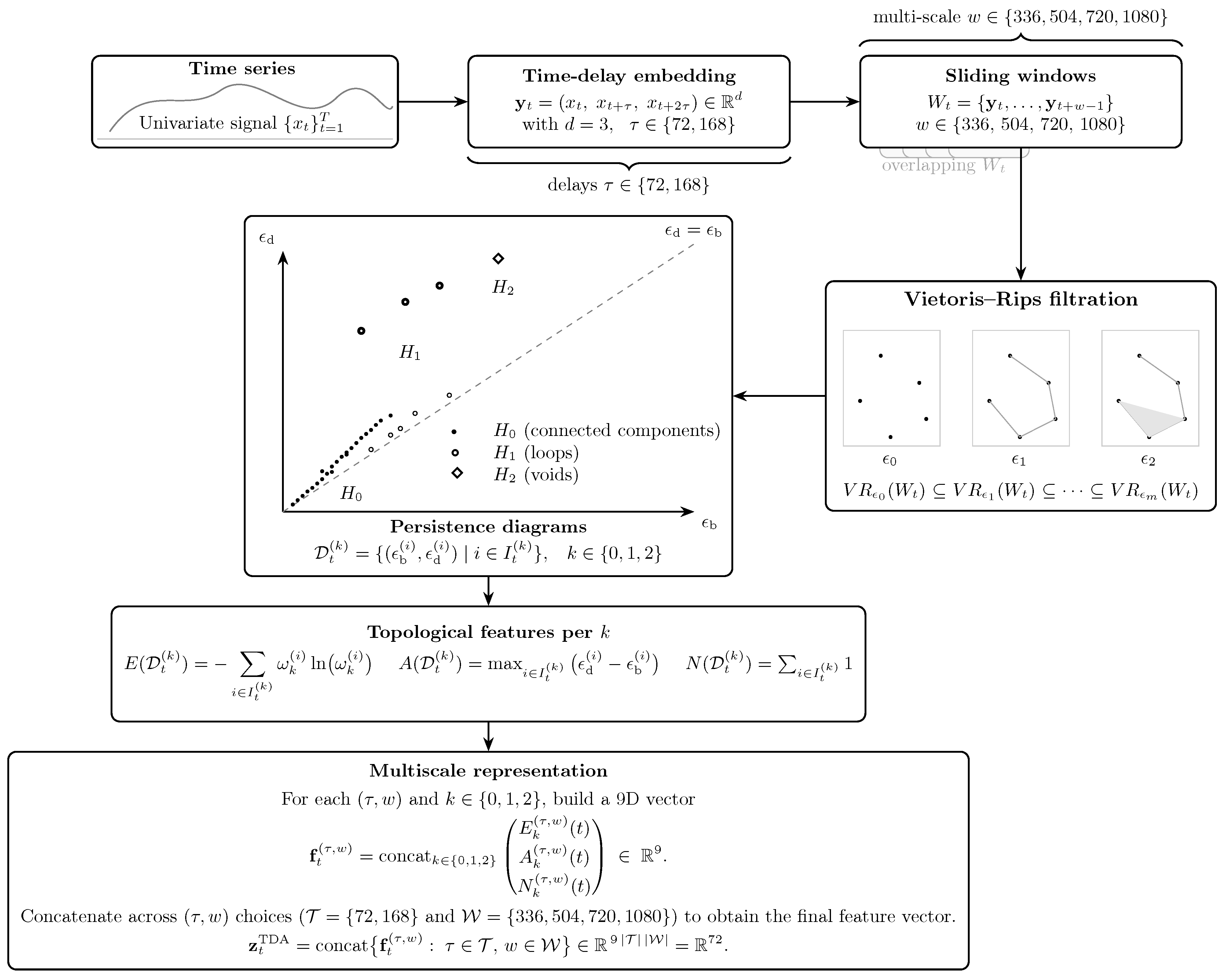
An overview of the proposed pipeline for topological feature extraction from time-series data is provided in Figure 1. The system’s phase space is reconstructed from a univariate time series, $\left\{x_t\right\}$ through time-delay embedding in ${\mathbb{R}}^3$ using multiple delays, $\tau$. The embedded trajectory is transformed by a sliding-window procedure of different lengths, w, into a collection of overlapping point clouds, $W_t$, each of which encodes a local dynamical structure. For each $W_t$, a Vietoris–Rips filtration is constructed, and persistent homology is computed, allowing the multiscale topological features of the point cloud to be captured through persistence diagrams, ${\mathcal{D}}_t^{\left(k\right)}$. From these diagrams, three summary statistics—persistence entropy, E, persistence amplitude, A, and the number of topological features, N—are extracted for each homology dimension, $k\in \{0,1,2\}$. Finally, a rich, multiscale topological representation of the time-series dynamics is obtained by concatenating these descriptors across different embedding delays and window sizes, making the representation suitable for subsequent analysis and modelling.

3.5. Integration with Downstream Tasks

Although the present study evaluates representations through structure-preservation criteria, rather than task-specific accuracy, the proposed multiscale topological descriptors are designed to be directly usable in downstream learning settings. The output of the pipeline is a compact, time-indexed multivariate sequence, $\left\{{\mathbf{z}}_t^{\mathrm{TDA}}\right\}$, that can be integrated into standard workflows without requiring specialised architectures.

3.5.1. Forecasting

In a predictive setting, ${\mathbf{z}}_t^{\mathrm{TDA}}$ can be used as a set of exogenous covariates (or combined with conventional temporal/spectral features) to predict future values $x_{t+h}$ at horizon h. Because each feature vector is computed from a causal sliding window of past embedded states, the representation can be extracted online (without look-ahead) and paired with lightweight learners (e.g., linear/regularised regression, tree-based models) or more expressive sequence models. In this interpretation, the topological features act as a multiscale summary of recent geometric organisation in phase space (connectivity, loops, cavities) that complements local statistics and frequency-domain descriptors.

3.5.2. Anomaly and Regime Detection

The same time-indexed representation naturally supports unsupervised monitoring tasks. Abrupt changes in the geometry of the embedded trajectory, such as the appearance/disappearance of persistent $H_1$ loops or shifts in $H_0$ merge scales, translate into detectable changes in ${\mathbf{z}}_t^{\mathrm{TDA}}$. This enables anomaly detection via distance-to-baseline or one-class methods in feature space, as well as change-point or regime detection by tracking distributional shifts of $\left\{{\mathbf{z}}_t^{\mathrm{TDA}}\right\}$ over time.

4. Experimental Framework

The experimental framework is designed to assess, in a model-agnostic manner, the extent to which TDA yields feature representations that preserve the intrinsic structure of real-world time series. The section proceeds as follows. First, the benchmark datasets are specified, emphasising the use of heterogeneous, regularly sampled financial series as challenging test beds (Section 4.1). Second, a deterministic preprocessing pipeline is detailed to produce a working signal suitable for topology-oriented analysis while respecting each asset’s native calendar (Section 4.2). Third, non-TDA baselines are introduced to contextualise TDA against alternative representations under an identical synthesis protocol and input handling (Section 4.3). Fourth, structure-preservation evaluation criteria are formalised (Section 4.4). Finally, the configuration of the TDA-based feature extractor is reported (Section 4.5).

4.1. Benchmark Datasets

The evaluation of the structure-preserving properties of TDA requires time series that exhibit heterogeneous temporal dynamics, well-defined regime shifts, and sufficient length to support robust statistical comparisons. To meet these criteria, financial daily price data were selected as benchmark signals. These data are not used for predictive modelling or decision-making; instead, they serve as challenging, diverse test cases to assess how well TDA-based feature representations retain the salient structural characteristics of the original series. Their availability, regular sampling, and rich dynamical behaviour make them well suited for this purpose.

Two complementary families of assets were considered to span a broad range of market mechanisms and statistical profiles. The first consists of six major cryptocurrencies quoted against USDT: BNBUSDT, BTCUSDT, ETHUSDT, XRPUSDT, ADAUSDT, and LTCUSDT. By quoting all assets against a stablecoin pegged to the US dollar, the confounding influence of base-currency fluctuations was reduced, allowing the intrinsic dynamics of the digital assets to be emphasised. The cryptocurrency data covers the period from January 2018 to January 2023. The second family consists of traditional financial instruments, chosen to complement the cryptocurrency set by including multiple sectors: the French CAC 40 equity index (FCHI), crude oil futures (CL = F, continuous series), the EUR/USD exchange rate (EURUSD), and the iShares Core MSCI Europe ETF (IEUR). For these instruments, data were collected from January 2023 to June 2024. A summary of the asset universe and sampling horizons is provided in

Table 1. Asset list, calendar, and sampling horizon used for structure-preservation evaluation.

Class	Symbol	Calendar	Span
Crypto	BNBUSDT	7-day	Jan 2018–Jan 2023
Crypto	BTCUSDT	7-day	Jan 2018–Jan 2023
Crypto	ETHUSDT	7-day	Jan 2018–Jan 2023
Crypto	XRPUSDT	7-day	Jan 2018–Jan 2023
Crypto	ADAUSDT	7-day	Jan 2018–Jan 2023
Crypto	LTCUSDT	7-day	Jan 2018–Jan 2023
Traditional	FCHI (CAC 40)	Business days	Jan 2023–Jun 2024
Traditional	CL=F (crude oil, continuous)	Business days	Jan 2023–Jun 2024
Traditional	EURUSD (FX)	Business days	Jan 2023–Jun 2024
Traditional	IEUR (ETF)	Business days	Jan 2023–Jun 2024

.

4.2. Data Preprocessing

Preprocessing was designed to prepare each time series for topology-oriented feature extraction and for the subsequent evaluation of structure preservation. All operations were performed per asset and on the asset’s native trading calendar so that the temporal structure to be preserved by TDA was not inadvertently altered by cross-asset alignment or calendar imputation choices. Timestamps were parsed into a consistent, timezone-free datetime index, and the analysis window was restricted to the spans defined in Section 4.1.

Missing values were handled by interpolation on the price domain using a cubic spline in continuous time. In concrete terms, the datetime index was mapped to a real-valued time axis using Unix timestamps. A subset of observed points was used to fit a cubic spline, and values at missing timestamps were evaluated from this spline. Non-finite values (NaN or $\pm \infty$) were treated as missing before interpolation. The resulting series was stored as the processed close, maintaining the original sampling grid and index.

To obtain a scale-stable working signal and to reduce low-frequency multiplicative effects, log-returns were computed from processed prices as $r_t=log\left(p_t\right)-log\left(p_{t-1}\right)$, with the first observation discarded. Outliers were then assessed diagnostically via standardised scores on $r_t$ and treated through winsorization, rather than deletion. Specifically, the empirical 2nd and 98th percentiles were used as lower and upper caps, producing a winsorised return ${\tilde{r}}_t=min\{max\{r_t,q_{0.02}\},q_{0.98}\}$. Stationarity was examined on the winsorised returns using the augmented Dickey–Fuller test with automatic lag selection by AIC and a 5% decision threshold. When the unit-root null could not be rejected, a first difference was applied to ${\tilde{r}}_t$ on a per-asset basis, after which stationarity was rechecked. When invoked, differencing was confined to maximal contiguous segments to avoid spurious reinitialisations around isolated gaps.

To mitigate scale effects in non-inherently scale-invariant metrics and distances, a linear normalisation to $[-1,1]$ was applied to the working return signal. Finally, for controlled multiscale smoothing and to construct non-topological reconstruction baselines, a maximal overlap discrete wavelet transform (MODWT) with a Daubechies-2 mother wavelet was applied to the normalised series at level 5. These bandwise reconstructions provide controlled levels of smoothing, which are later used to benchmark structure-preservation features against TDA-based reconstructions under matched sampling and alignment.

4.3. Non-TDA Baselines for Structure Preservation

To situate the proposed TDA-based representation within the structure-preservation problem, a set of non-TDA baseline feature extractors was assembled. All baselines operate on the identical inputs produced via the pipeline in Section 4.2, and a common, lightweight linear synthesis is used to project features back into signal space so that evaluation metrics are strictly comparable across methods; consequently, observed differences can be attributed to representational capacity, rather than modelling choices or data handling. The feature extractors considered are the following:

1.

Lagged Feature (LF). A concise, model-agnostic baseline is defined by stacking the lagged coordinates of the working univariate signal $\left\{x_t\right\}$ (cf. Section 4.2), using a lag index, ℓ. Let the day-based horizons be ${\mathcal{L}}_{\mathrm{day}}=\{1,3,7,14,21,30\}$ (trading days). For daily sampling,

$${\mathbf{z}}_t^{\mathrm{LF}}={concat}_{\mathsf{\ell }\in {\mathcal{L}}_{\mathrm{day}}}\left(\begin{array}{c}{x}_{t+\mathsf{\ell }-1}\end{array}\right)\in {\mathbb{R}}^6.$$

for $t=1,\dots ,T-max\left({\mathcal{L}}_{\mathrm{day}}\right)$. For hourly sampling, the same horizons are enforced with multiplier $f=24$, i.e., ${\mathcal{L}}_{\mathrm{hour}}=\{\mathsf{\ell }f:\mathsf{\ell }\in {\mathcal{L}}_{\mathrm{day}}\}=\{24,72,168,336,504,720\}$, and 

$${\mathbf{z}}_t^{\mathrm{LF}}={concat}_{\mathsf{\ell }\in {\mathcal{L}}_{\mathrm{hour}}}\left(\begin{array}{c}{x}_{t+\mathsf{\ell }-1}\end{array}\right)\in {\mathbb{R}}^6,$$

for $t=1,\dots ,T-max\left({\mathcal{L}}_{\mathrm{hour}}\right)$. Shifts are implemented as temporal displacements that (if applied to the full index) would introduce trailing missing values up to $max{\mathcal{L}}_{\mathrm{day}}$ (daily) or $max{\mathcal{L}}_{\mathrm{hour}}$ (hourly), thereby preserving alignment and preventing look-ahead in downstream uses by restricting t to the stated range. The selected horizons span immediate, weekly, biweekly, and monthly scales, providing a compact and interpretable representation of temporal dependencies across multiple time horizons.

2.

DateTime Features (DTFs). A concise, deterministic, calendar-driven feature set is defined by extracting calendar components from the timestamp attached to each observation of the working univariate signal $\left\{x_t\right\}$ (cf. Section 4.2). Let $\mathrm{ts}\left(t\right)$ denote the datetime index of $x_t$, and let $\mathrm{yr}, \mathrm{mo}, \mathrm{dom}, \mathrm{h}, \mathrm{dow}, \mathrm{doy}, \dim$ return, respectively, year, month, day of month, hour (0–23), day of week (Mon = 0, …, Sun = 6), day of year (1–365/366), and days in the month. For daily sampling (no hour component),

$${\mathbf{z}}_t^{\mathrm{DTF}}={\left(\mathrm{yr}\left(\mathrm{ts}\right(t\left)\right),\mathrm{mo}\left(\mathrm{ts}\right(t\left)\right),\mathrm{dom}\left(\mathrm{ts}\right(t\left)\right),\mathrm{dow}\left(\mathrm{ts}\right(t\left)\right),\mathrm{doy}\left(\mathrm{ts}\right(t\left)\right),\dim \left(\mathrm{ts}\right(t\left)\right)\right)}^{\top }.$$

For hourly sampling,

$${\mathbf{z}}_t^{\mathrm{DTF}}={\left(\mathrm{yr}\left(\mathrm{ts}\right(t\left)\right),\mathrm{mo}\left(\mathrm{ts}\right(t\left)\right),\mathrm{dom}\left(\mathrm{ts}\right(t\left)\right),\mathrm{h}\left(\mathrm{ts}\right(t\left)\right),\mathrm{dow}\left(\mathrm{ts}\right(t\left)\right),\mathrm{doy}\left(\mathrm{ts}\right(t\left)\right),\dim \left(\mathrm{ts}\right(t\left)\right)\right)}^{\top }.$$

Each ${\mathbf{z}}_t^{\mathrm{DTF}}$ is computed one-to-one with $x_t$ using only its timestamp (no external data and no look-ahead), yielding a compact, interpretable encoding of calendar regularities (yearly, seasonal, monthly, weekly, and intraday when applicable).

3.

Difference and Change Features (DCFs). A compact momentum-oriented feature set is defined by pairing rate-of-change and differences computed from the working univariate signal, $\left\{x_t\right\}$ (cf. Section 4.2). Let the day-based horizons be ${\mathcal{H}}_{\mathrm{day}}=\{1,3,7,14,21,30\}$. For $h\in {\mathcal{H}}_{\mathrm{day}}$,

$${\mathrm{ROC}}_h\left(t\right)={\displaystyle \frac{x_{t+max\left({\mathcal{H}}_{\mathrm{day}}\right)}}{x_{t+max\left({\mathcal{H}}_{\mathrm{day}}\right)-h}}}-1,{\Delta }_h\left(t\right)=x_{t+max\left({\mathcal{H}}_{\mathrm{day}}\right)}-x_{t+max\left({\mathcal{H}}_{\mathrm{day}}\right)-h},$$

for $t=1,\dots ,T-max\left({\mathcal{H}}_{\mathrm{day}}\right)$. Respectively, the daily feature vector is written compactly as

$${\mathbf{z}}_t^{\mathrm{DCF}}={concat}_{h\in {\mathcal{H}}_{\mathrm{day}}}\left(\begin{array}{c}{\mathrm{ROC}}_h\left(t\right)\\ {\Delta }_h\left(t\right)\end{array}\right)\in {\mathbb{R}}^{12}.$$

For hourly sampling, the same horizons are enforced via ${\mathcal{H}}_{\mathrm{hour}}=\{24,72,168,336,504,720\}$ (i.e., daily horizons scaled by $f=24$). For $m\in {\mathcal{H}}_{\mathrm{hour}}$,

$${\mathrm{ROC}}_m\left(t\right)={\displaystyle \frac{x_{t+max\left({\mathcal{H}}_{\mathrm{hour}}\right)}}{x_{t+max\left({\mathcal{H}}_{\mathrm{hour}}\right)-m}}}-1,{\Delta }_m\left(t\right)=x_{t+max\left({\mathcal{H}}_{\mathrm{hour}}\right)}-x_{t+max\left({\mathcal{H}}_{\mathrm{hour}}\right)-m},$$

for $t=1,\dots ,T-max\left({\mathcal{H}}_{\mathrm{hour}}\right)$. Finally, the hourly feature vector is

$${\mathbf{z}}_t^{\mathrm{DCF}}={concat}_{m\in {\mathcal{H}}_{\mathrm{hour}}}\left(\begin{array}{c}{\mathrm{ROC}}_m\left(t\right)\\ {\Delta }_m\left(t\right)\end{array}\right)\in {\mathbb{R}}^{12}.$$

This interleaved, horizon-indexed construction yields matched scale-invariant (ROC) and absolute-change ($\Delta$) components while preserving chronological alignment and avoiding look-ahead by restricting t to the stated ranges.

4.

Seasonal–Trend Loess Features (STLFs). An STL-based baseline is considered in which the observed series is represented by additive components with a fixed hourly seasonal period of 24, and robust estimation is used to limit the influence of extreme events. The trend component $m_t$ is obtained by locally weighted regression (LOESS), capturing persistent movements while filtering short-term fluctuations. The seasonal component $s_t$ is then isolated through iterative seasonal smoothing, using the most recent residual from the prior iteration to refine recurring patterns. The residual $r_t$ is finally formed as the remaining variation after removing trend and seasonality, thereby concentrating irregular, event-driven dynamics. The baseline feature vector at each time t is defined by the concatenation of these components,

$${\mathbf{z}}_t^{\mathrm{STLF}}=concat\left(\begin{array}{c}{m}_t\\ s_t\\ r_t\end{array}\right)\in {\mathbb{R}}^3.$$

5.

Time-Delay Embedding PCA (TDE-PCA). A compact comparison baseline is defined by combining time-delay embedding with principal component analysis (PCA) on the working univariate signal ${\left\{x_t\right\}}_{t=1}^T$ (cf. Section 4.2). The embedding dimension is fixed at $d=3$, and the delay varies over the day-based set $\mathcal{T}=\{1,3,7,14,21,30\}$. For hourly sampling, delays are scaled as ${\tau }_h=24\tau$ (hours). Thus, for a given $\tau \in \mathcal{T}$, the phase-space reconstruction forms

$${\mathbf{y}}_t^{\left(\tau \right)}={\left(x_t,x_{t+{\tau }_h},x_{t+2{\tau }_h}\right)}^{\top }\in {\mathbb{R}}^d,t=1,\dots ,T-(d-1){\tau }_h,$$

and stacks these row-wise into

$${\mathbf{Y}}^{\left(\tau \right)}=\left[\begin{array}{c}{\left({\mathbf{y}}_1^{\left(\tau \right)}\right)}^{\top }\\ ⋮\\ {\left({\mathbf{y}}_{T-(d-1){\tau }_h}^{\left(\tau \right)}\right)}^{\top }\end{array}\right]\in {\mathbb{R}}^{\left(T-(d-1){\tau }_h\right)\times d}.$$

After column-centring ${\mathbf{Y}}^{\left(\tau \right)}$, the first principal component direction ${\mathbf{w}}^{\left(\tau \right)}\in {\mathbb{R}}^d$ is obtained by a global PCA fit,

$${\mathbf{w}}^{\left(\tau \right)}=arg\underset{\parallel \mathbf{w}\parallel =1}{max}Var\left({\mathbf{Y}}^{\left(\tau \right)}\mathbf{w}\right),$$

and the one-dimensional embedded feature sequence is produced by

$$p_t^{\left(\tau \right)}={\left({\mathbf{y}}_t^{\left(\tau \right)}\right)}^{\top }{\mathbf{w}}^{\left(\tau \right)},t=1,\dots ,T-(d-1){\tau }_h.$$

Finally, the feature vector at each valid time, t, is formed by concatenation across delays,

$${\mathbf{z}}_t^{\mathrm{TDE}\text{-}\mathrm{PCA}}={concat}_{\tau \in \{1,3,7,14,21,30\}}\left(\begin{array}{c}{p}_t^{\left(\tau \right)}\end{array}\right)\in {\mathbb{R}}^6,$$

so that the six entries correspond, in order, to the first principal-component projections from embeddings with $\tau \in \{1,3,7,14,21,30\}$ (scaled to ${\tau }_h$ for hourly data).

6.

Price-Based Statistical Features (PBSFs). A parsimonious, interpretable baseline is constructed directly from OHLC prices aligned with the working index of ${\left\{x_t\right\}}_{t=1}^T$ (Section 4.2). Let $P_{\mathrm{close},t}$, $P_{\mathrm{high},t}$, $P_{\mathrm{low},t}$, and $P_{\mathrm{open},t}$ denote close, high, low, and open at time t. At each timestamp, the following elementary quantities are computed: logarithmic returns and percentage changes for each component, together with two range measures capturing intraday dispersion and open–close displacement—

$$\begin{array}{cccc}\hfill r_{\mathrm{close},t}& =log\left({\displaystyle \frac{P_{\mathrm{close},t}}{P_{\mathrm{close},t-1}}}\right),\hfill & \hfill {\Delta }_{\mathrm{close},t}& ={\displaystyle \frac{P_{\mathrm{close},t}-P_{\mathrm{close},t-1}}{P_{\mathrm{close},t-1}}},\hfill \\ \hfill r_{\mathrm{high},t}& =log\left({\displaystyle \frac{P_{\mathrm{high},t}}{P_{\mathrm{high},t-1}}}\right),\hfill & \hfill {\Delta }_{\mathrm{high},t}& ={\displaystyle \frac{P_{\mathrm{high},t}-P_{\mathrm{high},t-1}}{P_{\mathrm{high},t-1}}},\hfill \\ \hfill r_{\mathrm{low},t}& =log\left({\displaystyle \frac{P_{\mathrm{low},t}}{P_{\mathrm{low},t-1}}}\right),\hfill & \hfill {\Delta }_{\mathrm{low},t}& ={\displaystyle \frac{P_{\mathrm{low},t}-P_{\mathrm{low},t-1}}{P_{\mathrm{low},t-1}}},\hfill \\ \hfill r_{\mathrm{open},t}& =log\left({\displaystyle \frac{P_{\mathrm{open},t}}{P_{\mathrm{open},t-1}}}\right),\hfill & \hfill {\Delta }_{\mathrm{open},t}& ={\displaystyle \frac{P_{\mathrm{open},t}-P_{\mathrm{open},t-1}}{P_{\mathrm{open},t-1}}}.\hfill \end{array}$$

$${\mathrm{HLR}}_t=P_{\mathrm{high},t}-P_{\mathrm{low},t},{\mathrm{COR}}_t=P_{\mathrm{close},t}-P_{\mathrm{open},t}.$$

In alignment with the standard representation, the feature vector at time t is formed by stacking these ten quantities in fixed order,

$${\mathbf{z}}_t^{\mathrm{PBSF}}=concat\left(\begin{array}{c}{r}_{\mathrm{close},t}\\ r_{\mathrm{high},t}\\ r_{\mathrm{low},t}\\ r_{\mathrm{open},t}\\ {\Delta }_{\mathrm{close},t}\\ {\Delta }_{\mathrm{high},t}\\ {\Delta }_{\mathrm{low},t}\\ {\Delta }_{\mathrm{open},t}\\ {\mathrm{HLR}}_t\\ {\mathrm{COR}}_t\end{array}\right)\in {\mathbb{R}}^{10},$$

so that ${\mathbf{z}}_t^{\mathrm{PBSF}}$ provides a price-based summary combining directional changes (log-returns and percentage changes) with dispersion and displacement (high–low and close–open ranges) under strict chronological alignment.

7.

Feature Extraction Using Iterated Sums (FRUITS). A univariate hourly signal ${\left\{x_t\right\}}_{t=1}^T$ (Section 4.2) is processed by a sliding window of length $L=24\times 21$ (hours) with unit stride. For each window starting at index t, the samples are standardised in-window to stabilise scales:

$${\tilde{x}}_{t+i}={\displaystyle \frac{x_{t+i}-{\mu }_t}{{\sigma }_t}},{\mu }_t={\displaystyle \frac{1}{L}}\sum _{i=0}^{L-1}{x}_{t+i},{\sigma }_t^2={\displaystyle \frac{1}{L}}\sum _{i=0}^{L-1}{(x_{t+i}-{\mu }_t)}^2.$$

On the standardised trajectory $({\tilde{x}}_t,\dots ,{\tilde{x}}_{t+L-1})$, a FRUITS iterated-sum signature (ISS) is computed with dim$=1$, mode$=$EXTENDED, and words of weights $w\in \{1,2,3,4\}$. The END sieve is applied to obtain terminal values for each weight; the order-r component for the window beginning at t is denoted as ${\mathrm{ISS}}_r^{\mathrm{END}}\left(t\right)$. The four-dimensional feature vector is then defined as

$${\mathbf{z}}_t^{\mathrm{FRUITS}}=\left(\begin{array}{c}{\mathrm{ISS}}_1^{\mathrm{END}}\left(t\right)\\ {\mathrm{ISS}}_2^{\mathrm{END}}\left(t\right)\\ {\mathrm{ISS}}_3^{\mathrm{END}}\left(t\right)\\ {\mathrm{ISS}}_4^{\mathrm{END}}\left(t\right)\end{array}\right)\in {\mathbb{R}}^4,t=1,\dots ,T-L+1.$$

This construction yields a compact summary, invariant to monotone time reparameterisations up to the chosen order, capturing cumulative patterns from linear (weight 1) through fourth-order interactions (weight 4) over the last L observations.

The implementation of the FRUITS iterated-sum signature used in this study was obtained directly from the authors’ official GitHub repository (https://github.com/irkri/fruits, accessed on 1 December 2025).

8.

Network-Based Features (NetFs). From the hourly univariate signal ${\left\{x_t\right\}}_{t=1}^T$ (Section 4.2), a sliding window of length $L=24\times 21$ h with unit stride is applied. Within each window, three graphs are constructed passively: a weighted natural-visibility graph, a weighted horizontal-visibility graph, and a quantile-transition graph. For each graph, five standard network descriptors are computed: the average weighted degree, the average shortest path length, the clustering coefficient, the number of communities (Louvain), and modularity (Louvain). The feature vector associated with the window starting at index t is then formed by the concatenation of these fifteen values, ordered by graph (natural visibility, horizontal visibility, quantile); in this way, ${\mathbf{z}}_t^{\mathrm{NetF}}\in {\mathbb{R}}^{15}$ includes the five descriptors for each of the three graphs.

The implementation of the NetF network-based feature extraction method employed in this study was directly obtained from the authors’ official GitHub repository (https://github.com/vanessa-silva/NetF, accessed on 1 December 2025).

4.4. Performance Measures: Structural Preservation

In this section, the metrics used to assess the degree to which feature-space representations preserve the structure of the original series are described. The original univariate series is denoted as $\mathbf{x}={\left(x_t\right)}_{t\in \mathbb{Z}}$, and the multivariate feature series is denoted as

$$\mathbf{Z}={\left({\mathbf{z}}_t\right)}_{t\in \mathbb{Z}},{\mathbf{z}}_t={\left(z_t^{\left(1\right)},\dots ,z_t^{\left(d\right)}\right)}^{\top }\in {\mathbb{R}}^d,$$

with temporal alignment determined by the specific method. Three complementary performance measures are considered to quantify structural preservation:

1.

Spectral score (SS). Preservation of frequency–domain structure is quantified. In accordance with the implementation, a one-dimensional representative of $\mathbf{Z}$ is obtained by standardising the columns of $\mathbf{Z}$ and projecting onto the first principal component, which yields a scalar sequence $s_t$. The (raw) power spectral densities of $\mathbf{x}$ and of $s_t$ are computed separately via the periodogram, producing nonnegative arrays ${\left(P_x\left(f_k\right)\right)}_{k=1}^{K_x}$ and ${\left(P_s\left(f_k\right)\right)}_{k=1}^{K_s}$. Because the arrays may have different lengths, both spectra are aligned by truncation to a common length, $K=min(K_x,K_s)$, with the first K frequency bins retained; the truncated spectra are denoted as ${\mathbf{P}}_x={\left(P_x\left(f_k\right)\right)}_{k=1}^K$ and ${\mathbf{P}}_s={\left(P_s\left(f_k\right)\right)}_{k=1}^K$.

To compare spectral shapes independently of total power, each spectrum is normalised to a probability mass function through division by its sum:

$$p_k={\displaystyle \frac{P_x\left(f_k\right)}{{\sum }_{j=1}^K{P}_x\left(f_j\right)}},q_k={\displaystyle \frac{P_s\left(f_k\right)}{{\sum }_{j=1}^K{P}_s\left(f_j\right)}}.$$

Let $m_k=\frac{1}{2}(p_k+q_k)$. The natural logarithm is used to compute the Jensen–Shannon divergence:

$$D_{\mathrm{JS}}(p\parallel q)={\displaystyle \frac{1}{2}}\sum _{k=1}^K{p}_{k}log{\displaystyle \frac{p_k}{m_k}}+{\displaystyle \frac{1}{2}}\sum _{k=1}^K{q}_{k}log{\displaystyle \frac{q_k}{m_k}}\ge 0.$$

Finally, error-to-score mapping is applied to obtain a unit-interval score,

$$\mathrm{SS}(\mathbf{Z}\mid \mathbf{x})={\displaystyle \frac{1}{1+D_{\mathrm{JS}}(p\parallel q)}}\in (0,1],$$

and higher values indicate closer agreement between the normalised spectra of the original series and the PCA-based representative of the feature family.

2.

Mean Squared Error (MSE). For each feature family, a one-dimensional representative, $s_t$, is obtained by standardising the columns of $\mathbf{Z}$ and projecting onto the first principal component. The representative is then affinely re-scaled to match the empirical mean and standard deviation of the aligned original series $\mathbf{x}$, yielding the reconstruction.

$${\widehat{x}}_t={\sigma }_x{\displaystyle \frac{s_t-{\mu }_s}{{\sigma }_s}}+{\mu }_x,$$

where ${\mu }_s,{\sigma }_s$ are the mean and standard deviation of $s_t$, and ${\mu }_x,{\sigma }_x$ are those of $x_t$ (all computed on the standard, aligned sample); the mean squared error is calculated and normalised by the variance of $\mathbf{x}$:

$${\mathrm{MSE}}_{\mathrm{raw}}={\displaystyle \frac{1}{n}}\sum _{t=1}^n{\left(x_t-{\widehat{x}}_t\right)}^2,\mathrm{MSE}={\displaystyle \frac{{\mathrm{MSE}}_{\mathrm{raw}}}{\mathrm{Var}\left(\mathbf{x}\right)+\epsilon }},$$

with $\epsilon ={10}^{-10}$ for numerical stability.

3.

Statistical Moment score (SM). This criterion assesses the preservation of distributional moments (mean, standard deviation, skewness, excess kurtosis). In this metric, elements of $\mathbf{Z}$ are first standardised as ${\tilde{\mathbf{z}}}_t={\mathbf{D}}^{-1}({\mathbf{z}}_t-{\mathit{\mu }}_Z)$, with ${\mathit{\mu }}_Z\in {\mathbb{R}}^d$ being the empirical column means and $\mathbf{D}=\mathrm{diag}\left({\mathit{\sigma }}_Z\right)$. A one–dimensional summary is then obtained by principal–component projection: the sample covariance of ${\left\{{\tilde{\mathbf{z}}}_t\right\}}_{t\in \mathcal{Z}}$ is computed, its leading eigenvector is extracted, and each ${\tilde{\mathbf{z}}}_t$ is projected onto that direction to yield $s_t$. The sequence $\left\{s_t\right\}$ is subsequently affinely transformed to match the empirical mean and standard deviation of $\mathbf{x}$: it is centred and scaled using its own mean and standard deviation and then mapped to have mean ${\mu }_x$ and standard deviation ${\sigma }_x$. If the projection variance is zero, the reconstruction defaults to the constant series with value ${\mu }_x$. The resulting reconstructed series is denoted as $\widehat{\mathbf{x}}={\left({\widehat{x}}_t\right)}_{t\in \mathcal{Z}}$. Let $\mu (·)$, $\sigma (·)$, ${\gamma }_1(·)$ (skewness), and ${\gamma }_2(·)$ (excess kurtosis) denote empirical moments. The moment-wise relative errors, with stability constants ${\epsilon }_{\mu },{\epsilon }_{\sigma },{\epsilon }_{{\gamma }_1},{\epsilon }_{{\gamma }_2}>0$, are

$$e_{\mu }={\displaystyle \frac{|\mu \left(\widehat{\mathbf{x}}\right)-\mu \left(\mathbf{x}\right)|}{\left|\mu \left(\mathbf{x}\right)\right|+{\epsilon }_{\mu }}},e_{\sigma }={\displaystyle \frac{|\sigma \left(\widehat{\mathbf{x}}\right)-\sigma \left(\mathbf{x}\right)|}{\left|\sigma \left(\mathbf{x}\right)\right|+{\epsilon }_{\sigma }}},e_{{\gamma }_1}={\displaystyle \frac{|{\gamma }_1\left(\widehat{\mathbf{x}}\right)-{\gamma }_1\left(\mathbf{x}\right)|}{|{\gamma }_1\left(\mathbf{x}\right)|+{\epsilon }_{{\gamma }_1}}},e_{{\gamma }_2}={\displaystyle \frac{|{\gamma }_2\left(\widehat{\mathbf{x}}\right)-{\gamma }_2\left(\mathbf{x}\right)|}{|{\gamma }_2\left(\mathbf{x}\right)|+{\epsilon }_{{\gamma }_2}}}.$$

The average error is $\overline{e}=\frac{1}{4}(e_{\mu }+e_{\sigma }+e_{{\gamma }_1}+e_{{\gamma }_2})$, and the (unit-interval) score is

$$\mathrm{SM}(\mathbf{Z}\mid \mathbf{x})={\displaystyle \frac{1}{1+\overline{e}}}\in (0,1],$$

so that higher values denote a better preservation of location, scale, asymmetry, and tail shape relative to $\mathbf{x}$.

Across SS, MSE, and SM, a one-dimensional representative is obtained by standardising the columns of $\mathbf{Z}$ and projecting onto the first principal component. This PCA-based synthesis is adopted as a simple, fully deterministic, linear common projection for cross-family comparison, and it is not intended as an optimal reconstruction decoder; more expressive nonlinear alternatives would introduce additional modelling assumptions and hyperparameter tuning and are, therefore, deferred to future work. Furthermore, within this evaluation setting, structural preservation is treated as a notion of structural fidelity and does not imply preservation of task semantics, which remains objective-dependent (e.g., forecasting targets or anomaly labels). SS, MSE, and SM, therefore, serve as complementary proxies of retained structural information, capturing spectral similarity, variance-scaled reconstruction fidelity, and distributional shape.

Finally, it is essential to clarify that all family-level scores reported in tables and figures are standardised to the unit interval on a per-dataset (asset) and per-metric basis to ensure cross-family comparability. Specifically, after each raw metric has been computed, monotone min–max rescaling (with a slight numerical offset for numerical stability) is applied across feature families for that asset–metric pair. This post hoc transformation preserves the within-asset ordering of methods and affects only the scale and the offset.

4.5. Model Configuration for TDA-Based Feature Extraction

As indicated in the methodological section (Section 3), Vietoris–Rips persistent homology is computed up to $k=2$ on the time-delay embedding in ${\mathbb{R}}^3$. From each persistence diagram, ${\mathcal{D}}_t^{\left(k\right)}$, three descriptors are extracted—persistence entropy, E, persistence amplitude, A, and the number of features, N. Thus, for every $(\tau ,w)$ configuration, 9 TDA features (three descriptors for each $k\in \{0,1,2\}$) are obtained and later concatenated across configurations to form a multiscale vector, ${\mathbf{z}}_t^{\mathrm{TDA}}\in {\mathbb{R}}^{72}$.

The parameter grid is defined as $\tau \in \{72,168\}$ and $w\in \{336,504,720,1080\}$. Under an hourly sampling grid, $\tau =72$ corresponds to approximately 3 days and is, therefore, suited to exposing short-to-medium temporal dependencies (e.g., intraday spillovers and few-day momentum), whereas $\tau =168$ equals one week and is used to render weekly cyclicity and more sustained movements geometrically explicit in the embedding. The window sizes $w=336$ (≈2 weeks), $w=504$ (≈3 weeks), $w=720$ (≈1 month), and $w=1080$ (≈6 weeks) determine how many embedded states are included in each point cloud, $W_t$. Larger windows permit richer and more stable topological organisation to be detected (e.g., persistent loops or shell-like structures), while smaller windows emphasise local and transient structure.

5. Results and Discussion

5.1. Computational Results

In this section, results are reported concerning the structural-preservation information conveyed by the considered feature families relative to the original series, using the evaluation metrics defined above. The univariate target is contrasted with each multivariate representation on a per-feature-family basis.

Table 2. Summary statistics for the spectral score (SS) across tested feature families. Entries report ${\mathrm{mean}}_{\mathrm{std}}$ of the score and mean-rank_std over assets for the overall set, cryptocurrencies, and traditional assets.

	Overall		Cryptocurrencies Assets		Traditional Assets
	meanstd	rankstd	meanstd	rankstd	meanstd	rankstd
LF	${0.1135}_{0.069}$	${5.5000}_{2.173}$	${0.1624}_{0.031}$	${4.0000}_{0.894}$	${0.0402}_{0.030}$	${7.7500}_{1.258}$
DTFs	0.45620.462	3.80002.440	${0.0987}_{0.038}$	${5.5000}_{1.378}$	${\mathbf{0.9925}}_{\mathbf{0.015}}$	${\mathbf{1.2500}}_{\mathbf{0.500}}$
DCFs	${0.0159}_{0.018}$	${8.3000}_{0.675}$	${0.0147}_{0.016}$	${8.3333}_{0.516}$	${0.0176}_{0.023}$	${8.2500}_{0.957}$
STLFs	${0.1629}_{0.083}$	${4.6000}_{1.430}$	${0.1354}_{0.082}$	${5.0000}_{1.673}$	${0.2042}_{0.075}$	${4.0000}_{0.816}$
TDE-PCA	${0.1692}_{0.145}$	${4.9000}_{1.969}$	${0.1689}_{0.132}$	${4.6667}_{2.251}$	${0.1697}_{0.185}$	${5.2500}_{1.708}$
PBSFs	${0.1554}_{0.116}$	${5.1000}_{1.524}$	${0.0810}_{0.031}$	${6.1667}_{0.753}$	${0.2671}_{0.105}$	${3.5000}_{0.577}$
FRUITS	${0.0451}_{0.044}$	${7.6000}_{1.350}$	${0.0176}_{0.021}$	${8.3333}_{0.816}$	${0.0862}_{0.037}$	${6.5000}_{1.291}$
NetFs	${0.2873}_{0.204}$	${3.9000}_{2.644}$	0.43850.074	2.00000.000	${0.0605}_{0.047}$	${6.7500}_{1.708}$
TDA	${\mathbf{0.9546}}_{\mathbf{0.119}}$	${\mathbf{1.3000}}_{\mathbf{0.483}}$	${\mathbf{1.0000}}_{\mathbf{0.000}}$	${\mathbf{1.0000}}_{\mathbf{0.000}}$	0.88640.179	1.75000.500

presents the outcomes for the spectral score (SS) criterion, disaggregated by asset type—cryptocurrencies and traditional assets—and also aggregated overall across all assets. For each asset typology and method, two summaries are provided: (i) the empirical mean and standard deviation of the SS score, reported as ${\mathrm{mean}}_{\mathrm{std}}$, and (ii) the mean rank and its standard deviation, reported as ${\mathrm{rank}}_{\mathrm{std}}$. Ranks are computed within each asset by ordering the families from best (rank 1) to worst using average ranks for ties, and then averaged across assets in the corresponding group; the standard deviation reflects between–asset variability of the ranks. In the table, the best method in each block is shown in bold and the second best in italics.

As shown in Table 2, the proposed TDA demonstrates the strongest performance overall, achieving the best mean SS and the best mean rank across assets. A nuanced pattern arises in traditional assets, where DTFs appear to surpass TDA on both mean SS and mean rank, suggesting that calendar-driven components can be particularly informative for spectra shaped by trading schedules and market microstructure. Across the remaining baselines, performance is heterogeneous: NetFs and PBSFs perform competitively in specific settings, whereas DCFs and FRUITS remain consistently weaker on SS, in line with their limited capacity to retain oscillatory content under the present protocol.

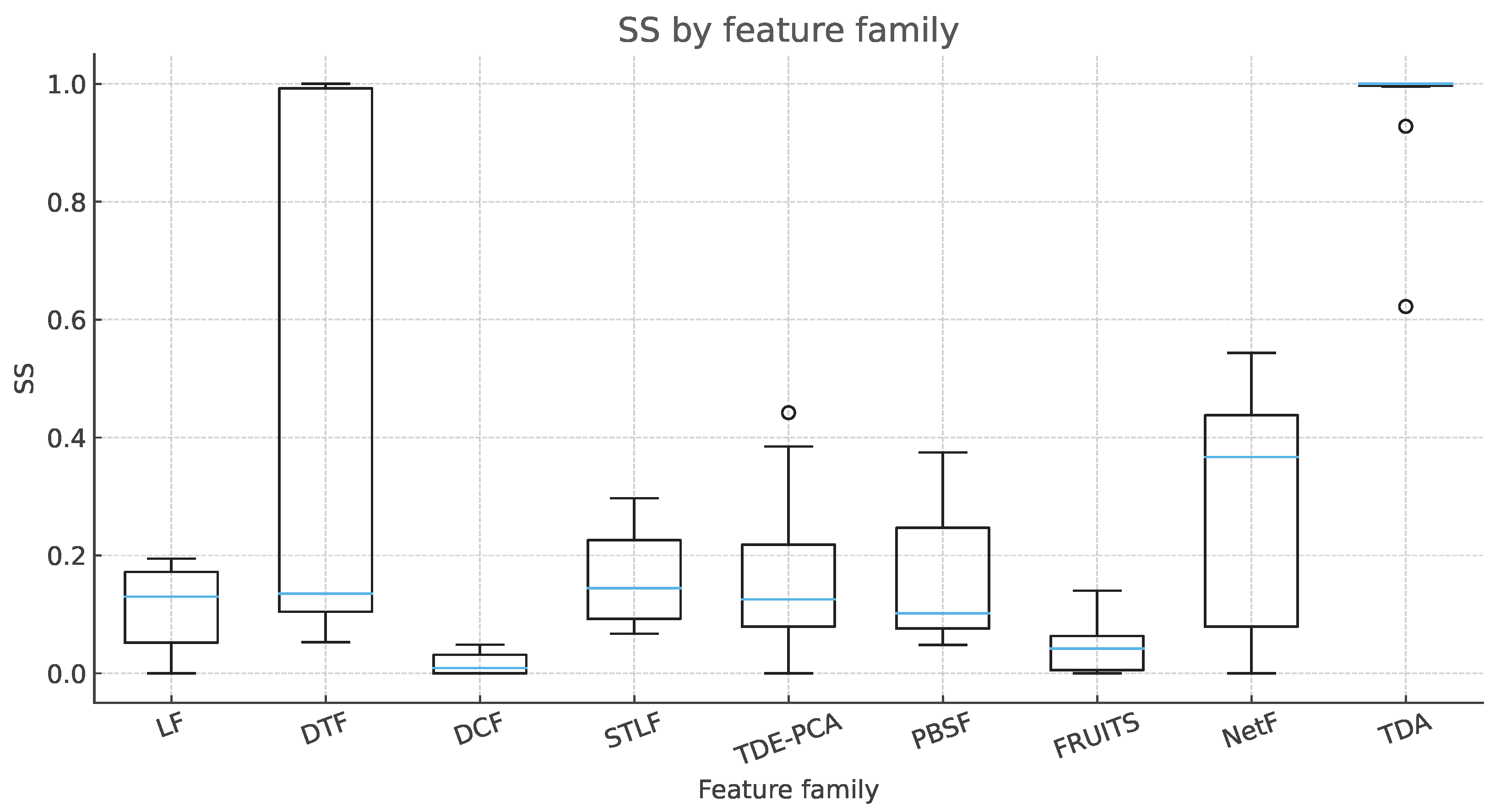
To complement these summaries, Figure 2 presents the distribution of SS via box–whisker plots. When the median (rather than the mean) is used as the measure of central tendency, the second most competitive family after TDA is NetFs, whose median SS is consistently high despite a wider interquartile range, indicating good typical performance with sensitivity to the asset class. This contrast between mean–based rankings (favouring DTFs in traditional assets) and median–based ordering (highlighting NetFs as the runner-up overall) underscores the presence of skewness and cross-asset heterogeneity in spectral preservation. Collectively, the box plots reaffirm TDA’s robust dominance while revealing distributional features that qualify the relative standing of non-topological baselines.

Second, an analysis analogous to the foregoing is conducted for the mean squared error (MSE), interpreted here as a reconstruction error; consequently, smaller values (closer to zero) are preferable. Detailed results are reported in

Table 3. Summary statistics for the mean squared error (MSE) across tested feature families. Entries report ${\mathrm{mean}}_{\mathrm{std}}$ of the error and mean-rank_std over assets for the overall set, cryptocurrencies, and traditional assets (lower is better).

	Overall		Cryptocurrencies Assets		Traditional Assets
	meanstd	rankstd	meanstd	rankstd	meanstd	rankstd
LF	${0.6189}_{0.239}$	${5.8000}_{1.989}$	${0.5850}_{0.226}$	${6.1667}_{2.041}$	${0.6698}_{0.282}$	${5.2500}_{2.062}$
DTFs	${\mathbf{0.2634}}_{\mathbf{0.312}}$	${\mathbf{3.0000}}_{\mathbf{2.789}}$	${\mathbf{0.2273}}_{\mathbf{0.195}}$	${\mathbf{2.8333}}_{\mathbf{2.229}}$	${\mathbf{0.3176}}_{\mathbf{0.472}}$	${\mathbf{3.2500}}_{\mathbf{3.862}}$
DCFs	${0.5373}_{0.224}$	${5.6000}_{1.955}$	${0.4331}_{0.146}$	${4.6667}_{1.966}$	${0.6935}_{0.246}$	${7.0000}_{0.816}$
STLFs	${0.6172}_{0.175}$	${6.5000}_{1.509}$	${0.5613}_{0.133}$	${6.1667}_{1.722}$	${0.7011}_{0.217}$	${7.0000}_{1.155}$
TDE-PCA	${0.4365}_{0.286}$	${3.8000}_{2.394}$	0.29930.225	3.00002.000	${0.6423}_{0.259}$	${5.0000}_{2.708}$
PBSFs	${0.5279}_{0.208}$	${4.7000}_{1.947}$	${0.4697}_{0.130}$	${4.5000}_{0.837}$	${0.6151}_{0.291}$	${5.0000}_{3.162}$
FRUITS	${0.5389}_{0.176}$	${4.8000}_{1.751}$	${0.4897}_{0.125}$	${5.3333}_{2.066}$	${0.6127}_{0.234}$	${4.0000}_{0.816}$
NetFs	${0.8103}_{0.231}$	${7.3000}_{2.263}$	${0.9102}_{0.142}$	${8.6667}_{0.516}$	${0.6606}_{0.277}$	${5.2500}_{2.363}$
TDA	0.38340.461	3.50003.598	${0.3719}_{0.487}$	${3.6667}_{3.777}$	0.40070.490	3.25003.862

for the overall sample, the subset of cryptocurrency assets, and the subset of traditional assets. In terms of averages, the proposed TDA is consistently competitive; however, DTFs attain the best mean MSE and the best mean rank overall and within the traditional segment, while TDA ranks second–best in both aggregations. Within cryptocurrencies, TDE–PCA exhibits the second–best average performance, and TDA remains close behind, indicating that delay–embedding with linear projections can be particularly effective when MSE is used to judge reconstruction fidelity. Collectively, the mean-based summaries suggest that calendar-driven regularities (DTFs) are especially beneficial for reducing the squared reconstruction error, with TDA providing a strong runner-up.

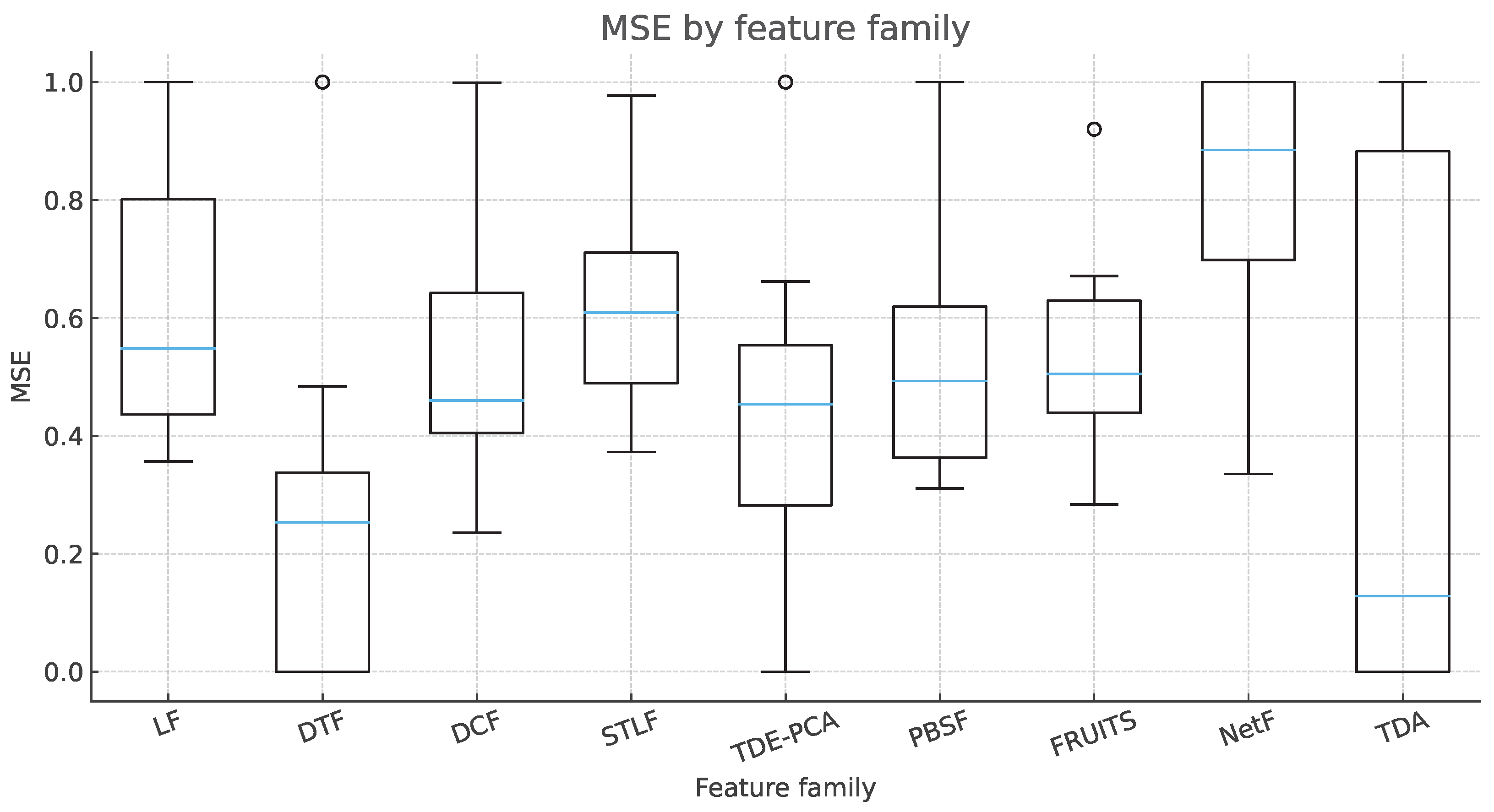
As the distributional perspective in Figure 3 shows, the median MSE (pooled across all assets) is the lowest for TDA, indicating the best typical reconstruction accuracy, whereas DTFs exhibit a smaller interquartile range (IQR), reflecting greater cross-asset stability around its central tendency. This pattern is consistent with a setting in which TDA achieves lower central errors but is more sensitive to asset heterogeneity or regime shifts, leading to a wider spread (and occasional larger errors). At the same time, DTFs deliver a more concentrated performance profile—likely driven by calendar regularities that generalise uniformly, albeit around a slightly higher median. Overall, TDA dominates in typical accuracy (lower median), whereas DTFs lead in dispersion (smaller IQR), highlighting a trade-off between central performance and variability.

In the final stage, an analysis analogous to the foregoing is conducted for the statistical moment score (SM), which assesses the preservation of low-order distributional moments (mean, standard deviation) and higher-order shape (skewness, kurtosis); higher values indicate better preservation. Detailed results are reported in

Table 4. Summary statistics for the statistical moment score (SM) across tested feature families. Entries report the ${\mathrm{mean}}_{\mathrm{std}}$ of the score and the mean-rank_std over assets for the overall set, cryptocurrencies, and traditional assets.

	Overall		Cryptocurrencies Assets		Traditional Assets
	meanstd	rankstd	meanstd	rankstd	meanstd	rankstd
LF	${0.6627}_{0.367}$	${3.8000}_{1.932}$	0.84550.129	3.00000.632	${0.3885}_{0.457}$	${5.0000}_{2.708}$
DTFs	${0.6864}_{0.174}$	${5.0000}_{2.000}$	${0.6387}_{0.214}$	${5.1667}_{2.041}$	${0.7580}_{0.055}$	${4.7500}_{2.217}$
DCFs	${0.5954}_{0.391}$	${4.8000}_{2.530}$	${0.7845}_{0.190}$	${3.6667}_{1.506}$	${0.3118}_{0.469}$	${6.5000}_{3.000}$
STLFs	${0.5261}_{0.329}$	${5.7000}_{2.452}$	${0.3570}_{0.181}$	${7.1667}_{0.408}$	${0.7798}_{0.358}$	3.50002.646
TDE-PCA	${0.6682}_{0.390}$	${3.6000}_{2.171}$	${0.7706}_{0.235}$	${3.1667}_{1.835}$	${0.5147}_{0.558}$	${4.2500}_{2.754}$
PBSFs	${0.4100}_{0.269}$	${6.6000}_{1.647}$	${0.2248}_{0.141}$	${7.8333}_{0.408}$	${0.6878}_{0.109}$	${4.7500}_{0.500}$
FRUITS	${0.0000}_{0.000}$	${9.0000}_{0.000}$	${0.0000}_{0.000}$	${9.0000}_{0.000}$	${0.0000}_{0.000}$	${9.0000}_{0.000}$
NetFs	0.84820.091	3.40001.713	${0.8109}_{0.077}$	${3.6667}_{1.506}$	${\mathbf{0.9042}}_{\mathbf{0.089}}$	${\mathbf{3.0000}}_{\mathbf{2.160}}$
TDA	${\mathbf{0.8642}}_{\mathbf{0.140}}$	${\mathbf{3.1000}}_{\mathbf{2.079}}$	${\mathbf{0.9142}}_{\mathbf{0.100}}$	${\mathbf{2.3333}}_{\mathbf{1.751}}$	0.78920.173	${4.2500}_{2.217}$

for the overall sample, cryptocurrencies, and traditional assets. In terms of averages, the proposed TDA attains the strongest overall performance and also leads within cryptocurrencies, while NetFs achieve the best mean and the best mean rank among traditional assets. Additional patterns are consistent with domain effects: LF is comparatively strong in cryptocurrencies, and TDE–PCA remains competitive across groups, whereas FRUITS is clearly the least competitive method in terms of moment preservation.

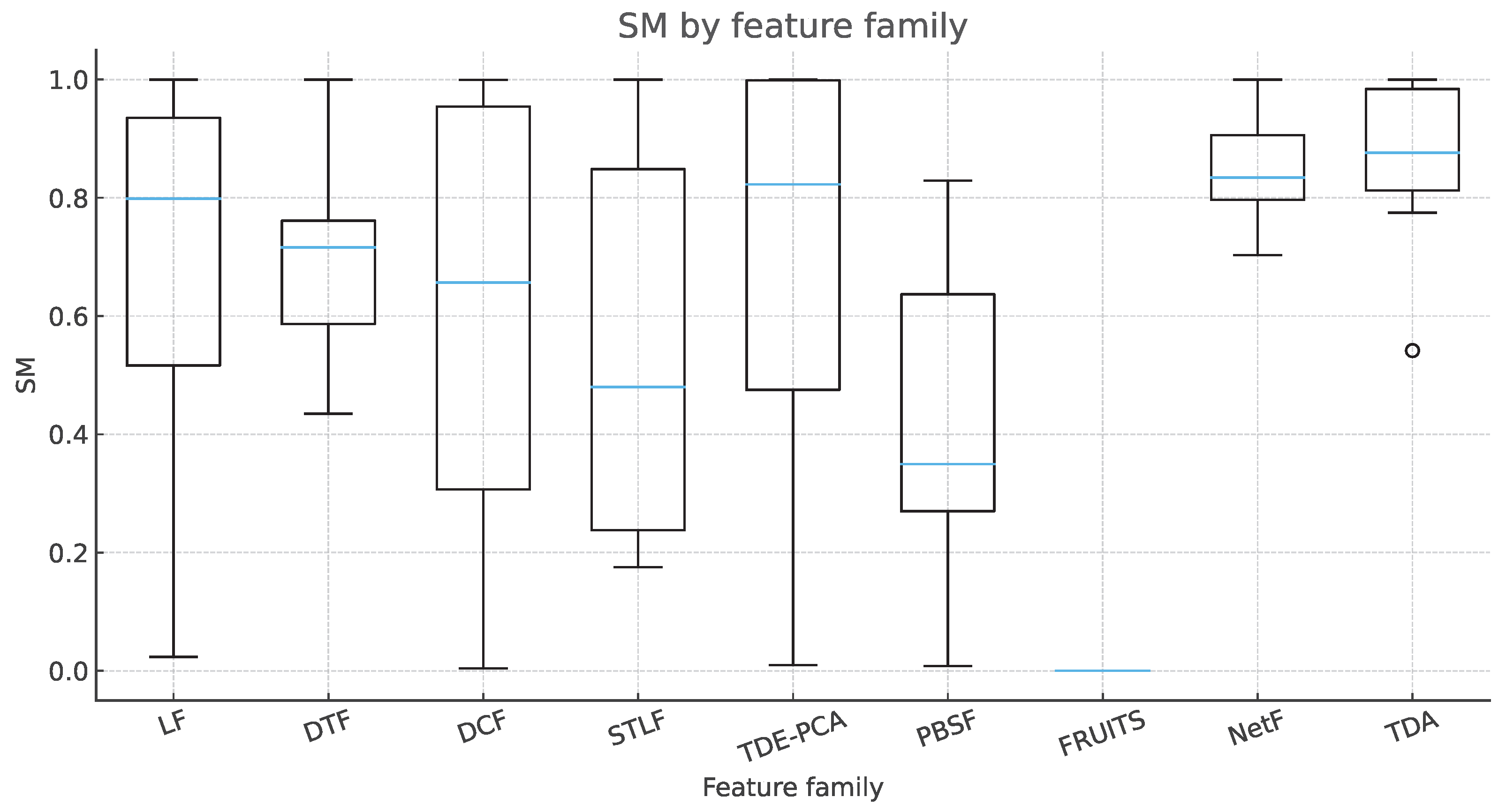
Turning to the distributional evidence in Figure 4, we find that the median SM is the highest for TDA, with NetFs emerging as the second most competitive family, TDE–PCA as the third, and LF as the fourth. Notably, TDA and NetFs stand out not only with their higher medians but also with their greater stability (narrower interquartile ranges) relative to the remaining families, indicating a robust preservation of moments across heterogeneous assets. This combination of superior central performance and reduced dispersion explains their consistent standing at the top of the distributional comparison.

Overall, the descriptive evidence indicates that the proposed TDA representation most reliably preserves structure across metrics and asset classes. For SS, TDA leads overall and in cryptocurrencies, while DTFs are strongest within traditional assets, consistent with calendar-driven spectral regularities. For MSE (reconstruction error), DTFs achieve the lowest mean, whereas TDA exhibits the lowest median with a wider spread, indicating better typical accuracy but greater cross-asset variability. For SM, TDA is best overall and in cryptocurrencies, with NetFs being comparatively strong in traditional assets. Collectively, these results position TDA as a broadly effective structural feature extractor, with domain-specific baselines (DTFs, NetFs, TDE–PCA) offering complementary strengths.

5.1.1. Inferential Evaluation of Structural Preservation

To complement the descriptive comparisons with an inferential evaluation, a nonparametric paired testing framework is adopted. The paired design is warranted because each feature family is assessed on the same set of assets, inducing within-asset coupling between TDA and each comparator and thereby controlling for cross–asset heterogeneity. A rank–based test is preferred over parametric alternatives to reduce sensitivity to heavy tails, heteroskedasticity, and non-Gaussian residual structures common in financial and nonlinear time-series data. Specifically, the two-sided Wilcoxon signed-rank test is applied to the vector of paired within-asset differences $\Delta =\mathrm{TDA}-\mathrm{family}$; for MSE (a loss to be minimised), the sign is inverted before testing so that, uniformly across metrics, positive differences favour TDA. Thus,

Table 5. Paired Wilcoxon signed-rank tests (by asset) comparing TDA against each feature family, reported per metric.

SS	LF	0.8450	0.0	0.0020 *°
SS	DTFs	0.8650	8.0	0.0488 *°
SS	DCFs	0.9777	0.0	0.0020 *°
SS	STLFs	0.8276	0.0	0.0020 *°
SS	TDE-PCA	0.8511	0.0	0.0020 *°
SS	PBSFs	0.8896	0.0	0.0020 *°
SS	FRUITS	0.9581	0.0	0.0020 *°
SS	NetFs	0.6021	0.0	0.0020 *°
MSE	LF	0.3705	15.0	$0.2324$
MSE	DTFs	−0.0099	22.0	0.6250
MSE	DCFs	0.2840	20.0	0.4922
MSE	STLFs	0.2911	13.0	0.1602
MSE	TDE-PCA	0.1772	24.0	0.7695
MSE	PBSFs	0.3895	21.0	0.5566
MSE	FRUITS	0.4196	20.0	0.4922
MSE	NetFs	0.4256	8.0	0.0488 *,°
SM	LF	0.1418	13.0	0.1602
SM	DTFs	0.1013	10.0	0.0840 °
SM	DCFs	0.2836	11.0	0.0955 °
SM	STLFs	0.3479	9.0	0.0645 °
SM	TDE-PCA	0.1177	16.0	0.2754
SM	PBSFs	0.4872	3.0	0.0098 *°
SM	FRUITS	0.8763	0.0	0.0020 *°
SM	NetFs	0.0741	22.0	0.6250

reports, for each metric and comparator, the Median diff. (the median of $\Delta$ across assets), the Wilcoxon statistic W, and the two–sided p-value. Values of p are annotated with * for $p\le 0.05$ and ° for $p\le 0.10$ (the latter subsumes the former), thereby separating the direction and magnitude of the effect (via the median difference) from strength of evidence (via W and p).

The inferential results are consistent and aligned with the descriptive evidence. For SS, all contrasts are strongly in favour of TDA (positive median differences; $p\approx 0.002$ throughout). For SM, TDA exhibits significant gains over FRUITS and PBSFs ($p\le 0.01$) and marginal advantages over DTFs, DCFs, and STLFs ($p\le 0.10$); the remaining contrasts are directionally favourable but not decisive at conventional levels. For MSE, only the comparison against NetFs reaches significance in favour of TDA ($p=0.0488$); the DTF contrast shows a small negative median difference ($-0.0099$) that is not significant ($p=0.625$). This last result coheres with the distributional analysis: although mean MSE is lower for DTFs, the box-plot comparison revealed a lower median MSE for TDA, indicating superior typical reconstruction at the expense of slightly greater dispersion. Taken together, the tests substantiate that TDA provides consistently superior structural preservation—median differences are positive against all families for SS and SM—and, except for the nonsignificant DTFs comparison in MSE, no statistically supported evidence contradicts TDA’s advantage.

5.1.2. Ablation Study

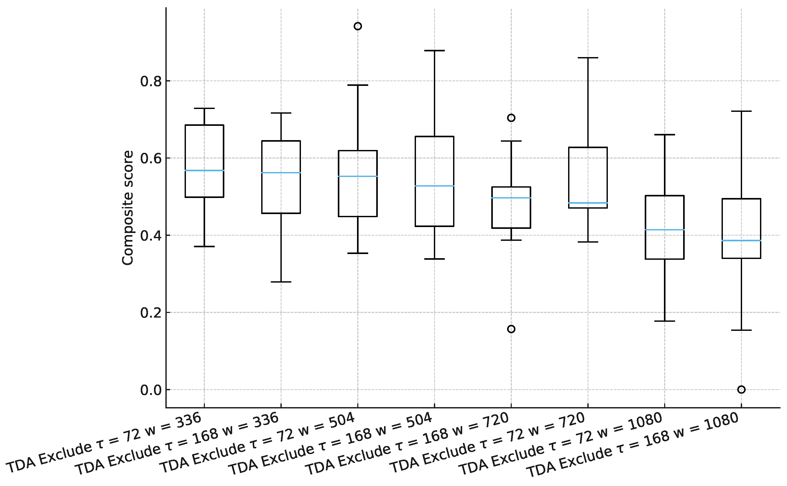
To conclude the experimental results, an ablation study was proposed in which, for each $(\tau ,w)$ configuration under consideration, the entire group of variables associated with that pair was removed. The objective was to assess how the exclusion of each such feature group influences the decline in model performance. To avoid unnecessary complexity while preserving a holistic view across metrics, performance was summarised by a single composite score, defined as the arithmetic mean of the three evaluation metrics (i.e., the mean of the three), computed after removing each group in turn.

The distribution of the composite score across ablations is shown in Figure 5 (box plots; one per $(\tau ,w)$ configuration). From these results, it is observed that the window length w constitutes the most influential determinant of performance: as w increases, larger declines in the composite score are obtained, indicating a stronger dependence on the excluded variables. The most pronounced degradations are observed at the upper bound of the window sizes considered ($w=1080$). With respect to the delay $\tau$, a comparatively modest effect is observed; descriptively, slightly better outcomes are associated with $\tau =168$ than with $\tau =72$.

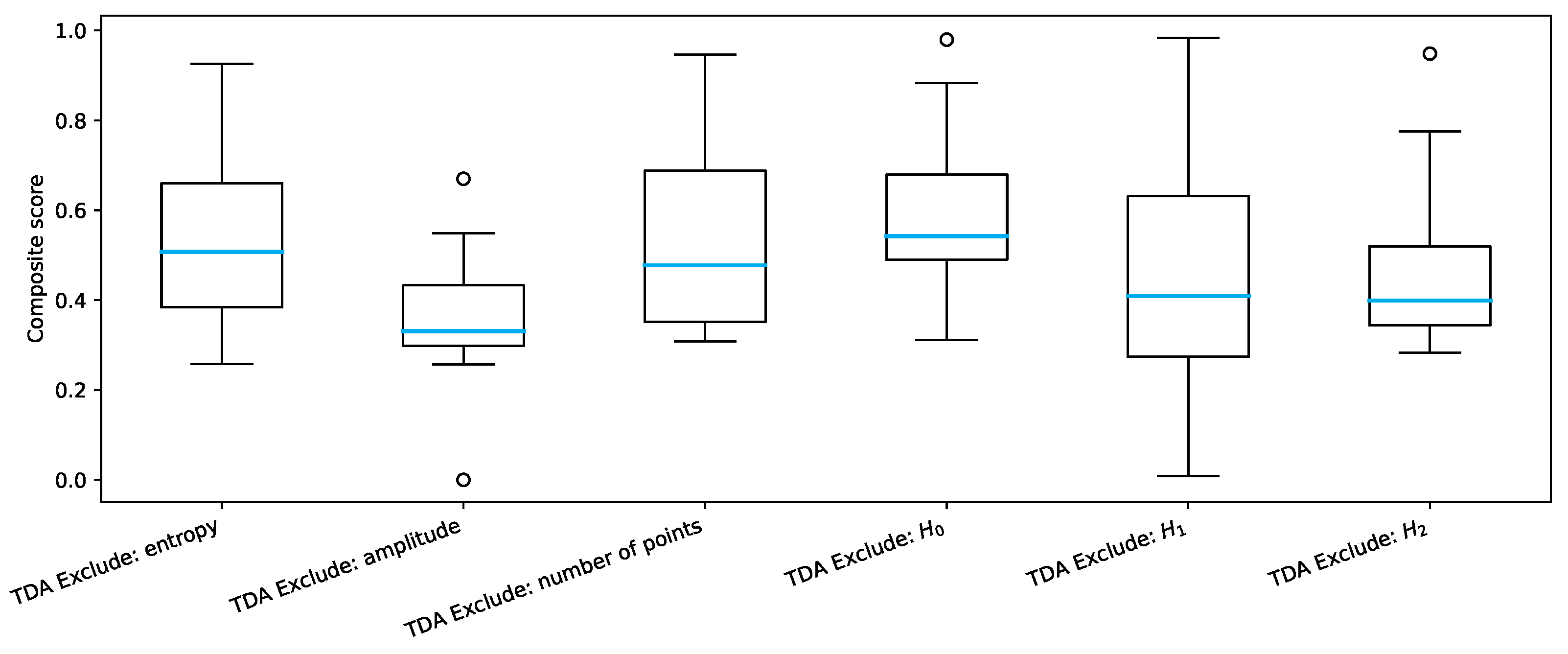
To further analyse which components of the multiscale TDA representation drive structural preservation, a complementary ablation was conducted by excluding entire groups of persistence-based descriptors. Two exclusion axes were considered: (i) the descriptor type (E, A, N) and (ii) the homology dimension ($H_0$, $H_1$, $H_2$). The resulting composite-score distributions are shown in Figure 6. Overall, the largest degradation is observed when amplitude-based descriptors (A) are removed, yielding the lowest median performance and indicating that maximum persistence carries the most influential topological signal under the present preservation criteria. Regarding homology dimensions, the lowest typical composite scores are observed when excluding $H_1$ and $H_2$, suggesting that these groups cause greater degradation in structural preservation than $H_0$. Moreover, the impact of excluding $H_1$ is markedly more heterogeneous across assets (wider dispersion) than that of excluding $H_2$, indicating stronger sensitivity to asset-specific dynamics.

5.1.3. Distance-Metric Sensitivity

To assess the sensitivity of the proposed TDA representation to the distance function used in the Vietoris–Rips filtration, an additional experiment was conducted by comparing three common choices: Euclidean (${\mathsf{\ell }}_2$), Manhattan (${\mathsf{\ell }}_1$), and Chebyshev (${\mathsf{\ell }}_{\infty }$). All remaining hyperparameters were held fixed ($d=3$, $\tau \in \{72,168\}$, $w\in \{336,504,720,1080\}$), and performance was evaluated with the same structural-preservation criteria (SS, MSE, SM). In addition, within this distance-sensitivity experiment, scores were min–max-normalised across distance variants (per asset and metric) to compare the relative effect of the distance metric. The summary in

Table 6. Distance-metric ablation for the VR filtration. Entries report the mean_std of the normalised scores and the mean rank in parentheses (lower is better). Best results in each column are highlighted in bold.

Distance	SS	MSE	SM	Composite
Euclidean (${\mathsf{\ell }}_2$)	${0.38}_{0.44}\left(2.30\right)$	${\mathbf{0.86}}_{\mathbf{0.31}}\left(\mathbf{1.60}\right)$	${0.57}_{0.44}\left(1.90\right)$	${\mathbf{0.61}}_{\mathbf{0.30}}\left(\mathbf{1.70}\right)$
Manhattan (${\mathsf{\ell }}_1$)	${\mathbf{0.61}}_{\mathbf{0.40}}\left(\mathbf{1.80}\right)$	${0.38}_{0.44}\left(2.20\right)$	${0.15}_{0.23}\left(2.60\right)$	${0.38}_{0.21}\left(2.30\right)$
Chebyshev (${\mathsf{\ell }}_{\infty }$)	${0.61}_{0.46}\left(1.90\right)$	${0.30}_{0.48}\left(2.20\right)$	${\mathbf{0.73}}_{\mathbf{0.38}}\left(\mathbf{1.50}\right)$	${0.55}_{0.30}\left(2.00\right)$

indicates that the Euclidean metric provides the strongest overall performance (best composite mean score and best mean rank), while Chebyshev is a competitive alternative when moment preservation is prioritised. Overall differences across metrics are moderate, supporting Euclidean distance as a robust default choice for the proposed pipeline.

5.1.4. Computational Burden

From a cost–performance perspective, the proposed representation remains compact (72 features per window) and is comparable in dimensionality to alternative multivariate summaries (e.g., NetFs with 15 features, FRUITS with 4, PBSFs with 10). The dominant computational cost arises from computing Vietoris–Rips persistent homology on each windowed point cloud of size w in ${\mathbb{R}}^3$. In practice, the per-window workload introduces a principled, model-agnostic framework for extracting and (ii) persistent-homology computation on the resulting filtration. Since homology is computed only up to dimension 2 (requiring simplices up to dimension 3), the number of simplices in the truncated VR complex admits a worst-case upper bound of $O\left(w^4\right)$, implying polynomial growth under this dimensional cap. By contrast, most non-topological baselines scale approximately linearly with the number of samples per window (e.g., lagged/calendar/difference features) or involve low-order transforms (e.g., STL and PCA-based embeddings). Overall, the extraction cost scales with the number of windows and the chosen window lengths, making w the primary driver of runtime and motivating the multiscale grid as a controllable trade-off between structural fidelity and computational expense. This yields a practical cost–performance compromise, since a larger w typically improves structural-preservation scores (SS, MSE, and SM) at the expense of a higher extraction cost.

5.2. Discussion: Practical Implications, Limitations, and Threats to Validity

This section discusses the results from a representation-centric perspective. Overall, the proposed TDA representation exhibits the strongest and most consistent structural preservation across heterogeneous assets, particularly in spectral similarity (SS) and distributional-shape preservation (SM). A key empirical observation is that calendar-driven DateTime features (DTFs) can outperform TDA in traditional assets under SS and mean MSE, likely reflecting strong market-calendar regularities and trading-schedule effects. In contrast, TDA remains robust across cryptocurrencies, where such calendar structure is weaker and multiscale geometric organisation plays a larger role.

From an interpretability standpoint, the ablation analyses suggest that maximum persistence amplitude carries the most influential signal and that higher-dimensional features ($H_1$ and $H_2$) contribute more strongly to preservation than $H_0$ under the present criteria. This indicates that loops and cavities in reconstructed phase space may encode meaningful multiscale organisation not easily captured by non-topological baselines.

5.2.1. Limitations and Threats to Validity

The current study relied on a fixed embedding dimension ($d=3$) and a fixed grid of delays and window sizes, which were selected for interpretability and tractability, rather than global optimality. In addition, Vietoris–Rips persistent homology may be sensitive to sampling density and noise, and the PCA-based synthesis used for cross-family reconstruction is intentionally a simple common decoder, rather than an optimal projection. These limitations motivate future work on adaptive hyperparameter selection, alternative filtrations, and nonlinear decoding strategies when task-specific reconstruction is desired.

5.2.2. Scope

Finally, structural preservation scores quantify fidelity in spectral, reconstruction, and distributional terms but do not guarantee the preservation of task semantics (e.g., forecasting utility or anomaly labels), which remain objective-dependent.

6. Conclusions

This study has introduced a principled, model-agnostic framework for extracting structural features from time series via topological data analysis (TDA). A multiscale pipeline was developed that reconstructs the phase space through time–delay embeddings, computes Vietoris–Rips persistent homology up to dimension $k=2$, and summarises persistence diagrams by entropy, amplitude, and feature counts across multiple delays and window sizes. The resulting multivariate representation was benchmarked against a diverse set of non-topological baselines (LF, DTFs, DCFs, STLFs, TDE–PCA, PBSFs, FRUITS, NetFs) under a unified preprocessing and evaluation protocol. Structural preservation was assessed with three complementary criteria: the spectral score (SS), the mean squared error (MSE; lower is better), and the statistical moment score (SM). Descriptively, TDA exhibited the most reliable structure retention across metrics and asset classes: it dominated SS (best mean and rank across all groups). For SM, it ranked the best overall and within cryptocurrencies, with NetFs being the strongest in traditional assets. For MSE, DTFs achieved the lowest mean error, whereas TDA attained the lowest median with a broader spread. These descriptive patterns were corroborated by paired Wilcoxon signed–rank tests by asset: median differences favoured TDA across all families for SS with uniformly significant p-values; and for SM, TDA showed statistically significant gains over FRUITS and PBSFs and marginal advantages over DTFs, DCFs, and STLFs; for MSE, only the contrast against NetFs was substantial in favour of TDA, while the TDA–DTF difference was slight and not substantial—consistent with the observed trade-off between a lower median error (TDA) and tighter dispersion (DTFs).

Future work will extend the topological representation along several dimensions. First, adaptive hyperparameter selection (embedding dimension, delays, window lengths) and data-driven filtrations (e.g., alpha complexes, witness complexes) will be explored to improve robustness and scalability. Second, downstream tasks such as forecasting, change-point detection, and regime classification will be considered to examine how topological features interact with task-specific objectives. Third, cross-domain validation beyond financial series (e.g., physiological, environmental, industrial signals) will be pursued to test generality. The limitations of the present study include the reliance on a fixed embedding dimension and VR filtrations, the potential sensitivity of persistence statistics to sampling density and noise, and the focus on summary descriptors, rather than whole diagram-based kernels or distances. Addressing these aspects may further strengthen the empirical advantages of TDA while clarifying the conditions under which topological structure offers the greatest practical benefit.

References

1. Nikolaou, A.; Gutiérrez, P.A.; Durán, A.; Dicaire, I.; Fernández-Navarro, F.; Hervás-Martínez, C. Detection of early warning signals in paleoclimate data using a genetic time series segmentation algorithm. Clim. Dyn. 2015, 44, 1919–1933. [Google Scholar] [CrossRef] [Scilit]
2. Fernández-Navarro, F.; de la Cruz, M.A.; Gutiérrez, P.A.; Castaño, A.; Hervás-Martínez, C. Time series forecasting by recurrent product unit neural networks. Neural Comput. Appl. 2018, 29, 779–791. [Google Scholar] [CrossRef] [Scilit]
3. Pérez-Ortiz, M.; Duran-Rosal, A.M.; Gutiérrez, P.A.; Sanchez-Monedero, J.; Nikolaou, A.; Fernández-Navarro, F.; Hervás-Martínez, C. On the use of evolutionary time series analysis for segmenting paleoclimate data. Neurocomputing 2019, 326, 3–14. [Google Scholar] [CrossRef] [Scilit]
4. Li, L.; Wu, Y.; Ou, Y.; Li, Q.; Zhou, Y.; Chen, D. Research on machine learning algorithms and feature extraction for time series. In Proceedings of the 2017 IEEE 28th Annual International Symposium on Personal, Indoor, and Mobile Radio Communications (PIMRC), Montreal, QC, Canada, 8–13 October 2017; pp. 1–5. [Google Scholar] [CrossRef] [Scilit]
5. Silva, V.F.; Silva, M.E.; Ribeiro, P.; Silva, F. Novel features for time series analysis: A complex networks approach. Data Min. Knowl. Discov. 2022, 36, 1062–1101. [Google Scholar] [CrossRef] [Scilit]
6. Baldán, F.J.; Benítez, J.M. Complexity measures and features for times series classification. Expert Syst. Appl. 2023, 213, 119227. [Google Scholar] [CrossRef] [Scilit]
7. Fulcher, B.D. Feature-Based Time-Series Analysis. In Feature Engineering for Machine Learning and Data Analytics; Dong, G., Liu, H., Eds.; CRC Press: Boca Raton, FL, USA, 2018; pp. 87–116. [Google Scholar] [CrossRef] [Scilit]
8. Lubba, C.H.; Sethi, S.S.; Knaute, P.; Schultz, S.R.; Fulcher, B.D.; Jones, N.S. catch22: CAnonical Time-series CHaracteristics: Selected through highly comparative time-series analysis. Data Min. Knowl. Discov. 2019, 33, 1821–1852. [Google Scholar] [CrossRef] [Scilit]
9. Henderson, T.; Fulcher, B.D. An Empirical Evaluation of Time-Series Feature Sets. In Proceedings of the 2021 International Conference on Data Mining Workshops (ICDMW), Auckland, New Zealand, 7–10 December 2021; pp. 1032–1038. [Google Scholar] [CrossRef] [Scilit]
10. Christ, M.; Braun, N.; Neuffer, J.; Kempa-Liehr, A.W. Time series feature extraction on basis of scalable hypothesis tests (tsfresh—A python package). Neurocomputing 2018, 307, 72–77. [Google Scholar] [CrossRef] [Scilit]
11. Barandas, M.; Folgado, D.; Fernandes, L.; Santos, S.; Abreu, M.; Bota, P.; Liu, H.; Schultz, T.; Gamboa, H. TSFEL: Time series feature extraction library. SoftwareX 2020, 11, 100456. [Google Scholar] [CrossRef] [Scilit]
12. Mothilall, D.; Van Zyl, T. An evaluation of the Long Short-Term Memory model for predictive maintenance applications in the aircraft industry. In Proceedings of the 2024 International Conference on Artificial Intelligence, Computer, Data Sciences and Applications (ACDSA), Victoria, Seychelles, 1–2 February 2024; pp. 1–5. [Google Scholar] [CrossRef] [Scilit]
13. Renault, A.; Bondu, A.; Lemaire, V.; Gay, D. Automatic feature engineering for time series classification: Evaluation and discussion. In Proceedings of the 2023 International Joint Conference on Neural Networks (IJCNN), Gold Coast, Australia, 18–23 June 2023; pp. 1–10. [Google Scholar] [CrossRef] [Scilit]
14. Kang, Y.; Hyndman, R.J.; Smith-Miles, K. Visualising forecasting algorithm performance using time series instance spaces. Int. J. Forecast. 2017, 33, 345–358. [Google Scholar] [CrossRef] [Scilit]
15. Deng, H.; Runger, G.; Tuv, E.; Vladimir, M. A time series forest for classification and feature extraction. Inf. Sci. 2013, 239, 142–153. [Google Scholar] [CrossRef] [Scilit]
16. Cabello, N.; Naghizade, E.; Qi, J.; Kulik, L. Fast and accurate time series classification through supervised interval search. In Proceedings of the 2020 IEEE International Conference on Data Mining (ICDM), Sorrento, Italy, 17–20 November 2020; pp. 948–953. [Google Scholar] [CrossRef] [Scilit]
17. Cabello, N.; Naghizade, E.; Qi, J.; Kulik, L. Fast, accurate and explainable time series classification through randomization. Data Min. Knowl. Discov. 2024, 38, 748–811. [Google Scholar] [CrossRef] [Scilit]
18. Mallat, S.G. A theory for multiresolution signal decomposition: The wavelet representation. IEEE Trans. Pattern Anal. Mach. Intell. 2002, 11, 674–693. [Google Scholar] [CrossRef] [Scilit]
19. Zhao, Q.; Lai, F.; Mo, X. Exploring time series analysis in frequency domain with complex-valued spectral attention and bidirectional variable mamb. J. Supercomput. 2025, 81, 875. [Google Scholar] [CrossRef] [Scilit]
20. Cuesta-Frau, D. Using the information provided by forbidden ordinal patterns in permutation entropy to reinforce time series discrimination capabilities. Entropy 2020, 22, 494. [Google Scholar] [CrossRef] [Scilit] [PubMed]
21. Pessa, A.A.; Ribeiro, H.V. ordpy: A Python package for data analysis with permutation entropy and ordinal network methods. Chaos Interdiscip. J. Nonlinear Sci. 2021, 31, 063110. [Google Scholar] [CrossRef] [Scilit]
22. Lacasa, L.; Luque, B.; Ballesteros, F.; Luque, J.; Nuno, J.C. From time series to complex networks: The visibility graph. Proc. Natl. Acad. Sci. USA 2008, 105, 4972–4975. [Google Scholar] [CrossRef] [Scilit]
23. Long, W.; Lu, Z.; Cui, L. Deep learning-based feature engineering for stock price movement prediction. Knowl.-Based Syst. 2019, 164, 163–173. [Google Scholar] [CrossRef] [Scilit]
24. Hao, Y.; Cao, H. A New Attention Mechanism to Classify Multivariate Time Series. In Proceedings of the Twenty-Ninth International Joint Conference on Artificial Intelligence, IJCAI-20; Bessiere, C., Ed.; International Joint Conferences on Artificial Intelligence Organization: Marina del Rey, CA, USA, 2020; pp. 1999–2005. [Google Scholar] [CrossRef] [Scilit]
25. Wu, J.; Xu, K.; Chen, X.; Li, S.; Zhao, J. Price graphs: Utilizing the structural information of financial time series for stock prediction. Inf. Sci. 2022, 588, 405–424. [Google Scholar] [CrossRef] [Scilit]
26. Qu, K.; Xue, S.; Zheng, X.; Yan, D.; Cao, H. Learning dynamic inter-farm dependencies for wind power forecasting via adaptive sparse graph attention network. Renew. Energy 2025, 258, 124969. [Google Scholar] [CrossRef] [Scilit]
27. Wu, Z.; Pan, S.; Long, G.; Jiang, J.; Chang, X.; Zhang, C. Connecting the Dots: Multivariate Time Series Forecasting with Graph Neural Networks. In Proceedings of the 26th ACM SIGKDD International Conference on Knowledge Discovery & Data Mining (KDD’20), Virtual Event, 23–27 August 2020; pp. 753–763. [Google Scholar] [CrossRef] [Scilit]
28. Cui, Y.; Zheng, K.; Cui, D.; Xie, J.; Deng, L.; Huang, F.; Zhou, X. METRO: A Generic Graph Neural Network Framework for Multivariate Time Series Forecasting. Proc. VLDB Endow. 2022, 15, 224–236. [Google Scholar] [CrossRef] [Scilit]
29. Jin, M.; Koh, H.Y.; Wen, Q.; Zambon, D.; Alippi, C.; Webb, G.I.; King, I.; Pan, S. A Survey on Graph Neural Networks for Time Series: Forecasting, Classification, Imputation, and Anomaly Detection. IEEE Trans. Pattern Anal. Mach. Intell. 2024, 46, 10466–10485. [Google Scholar] [CrossRef] [Scilit]
30. Ye, L.; Keogh, E. Time series shapelets: A new primitive for data mining. In Proceedings of the 15th ACM SIGKDD International Conference on Knowledge Discovery and Data Mining (KDD ’09), Paris, France, 28 June–1 July 2009; pp. 947–956. [Google Scholar] [CrossRef] [Scilit]
31. Grabocka, J.; Schilling, N.; Wistuba, M.; Schmidt-Thieme, L. Learning time-series shapelets. In Proceedings of the 20th ACM SIGKDD International Conference on Knowledge Discovery and Data Mining (KDD ’14), New York, NY, USA, 24–27 August 2014; pp. 392–401. [Google Scholar] [CrossRef] [Scilit]
32. Lin, J.; Khade, R.; Li, Y. Rotation-invariant similarity in time series using bag-of-patterns representation. J. Intell. Inf. Syst. 2012, 39, 287–315. [Google Scholar] [CrossRef] [Scilit]
33. He, Z.; Long, S.; Ma, X.; Zhao, H. A Boundary Distance-Based Symbolic Aggregate Approximation Method for Time Series Data. Algorithms 2020, 13, 284. [Google Scholar] [CrossRef] [Scilit]
34. Schäfer, P.; Leser, U. Fast and Accurate Time Series Classification with WEASEL. In Proceedings of the 2017 ACM on Conference on Information and Knowledge Management (CIKM ’17), Singapore, 6–10 November 2017; pp. 637–646. [Google Scholar] [CrossRef] [Scilit]
35. Bagnall, A.; Lines, J.; Bostrom, A.; Large, J.; Keogh, E. The great time series classification bake off: A review and experimental evaluation of recent algorithmic advances. Data Min. Knowl. Discov. 2017, 31, 606–660. [Google Scholar] [CrossRef] [Scilit]
36. Dempster, A.; Schmidt, D.F.; Webb, G.I. MiniRocket: A Very Fast (Almost) Deterministic Transform for Time Series Classification. In Proceedings of the 27th ACM SIGKDD Conference on Knowledge Discovery & Data Mining, Singapore, 14–18 August 2021; pp. 248–257. [Google Scholar] [CrossRef] [Scilit]
37. Tan, C.W.; Dempster, A.; Bergmeir, C.; Webb, G.I. MultiRocket: Multiple pooling operators and transformations for fast and effective time series classification. Data Min. Knowl. Discov. 2022, 36, 1623–1646. [Google Scholar] [CrossRef] [Scilit]
38. Eltrass, A.S.; Tayel, M.B.; Ammar, A.I. Automated ECG multi-class classification system based on combining deep learning features with HRV and ECG measures. Neural Comput. Appl. 2022, 34, 8755–8775. [Google Scholar] [CrossRef] [Scilit]
39. Qiu, Y.; Guo, H.; Wang, S.; Yang, S.; Peng, X.; Xiayao, D.; Chen, R.; Yang, J.; Liu, J.; Li, M.; et al. Deep learning-based multimodal fusion of the surface ECG and clinical features in prediction of atrial fibrillation recurrence following catheter ablation. BMC Med. Inform. Decis. Mak. 2024, 24, 225. [Google Scholar] [CrossRef] [Scilit]
40. Fermanian, A.; Lyons, T.; Morrill, J.; Salvi, C. New Directions in the Applications of Rough Path Theory. IEEE BITS Inf. Theory Mag. 2023, 3, 41–53. [Google Scholar] [CrossRef] [Scilit]
41. Diehl, J.; Krieg, R. FRUITS: Feature extraction using iterated sums for time series classification. Data Min. Knowl. Discov. 2024, 38, 4122–4156. [Google Scholar] [CrossRef] [Scilit]
42. Fulcher, B.D.; Little, M.A.; Jones, N.S. Highly comparative time-series analysis: The empirical structure of time series and their methods. J. R. Soc. Interface 2013, 10, 20130048. [Google Scholar] [CrossRef] [Scilit]
43. Fulcher, B.D.; Jones, N.S. hctsa: A computational framework for automated time-series phenotyping using massive feature extraction. Cell Syst. 2017, 5, 527–531. [Google Scholar] [CrossRef] [Scilit]
44. Santos, M.; Cerqueira, V.; Soares, C. Benchmarking Time Series Feature Extraction for Algorithm Selection. In Proceedings of the EPIA Conference on Artificial Intelligence; Springer: Berlin/Heidelberg, Germany, 2025; pp. 269–281. [Google Scholar] [CrossRef] [Scilit]
45. Talagala, T.S.; Hyndman, R.J.; Athanasopoulos, G. Meta-learning how to forecast time series. J. Forecast. 2023, 42, 1476–1501. [Google Scholar] [CrossRef] [Scilit]
46. Baydogan, M.G.; Runger, G. Time series representation and similarity based on local autopatterns. Data Min. Knowl. Discov. 2016, 30, 476–509. [Google Scholar] [CrossRef] [Scilit]
47. Abril, F.; Quimbay, C. Evolution of temporal fluctuation scaling exponent in nonstationary time series using supersymmetric theory of stochastic dynamics. Phys. Rev. E 2024, 109, 024112. [Google Scholar] [CrossRef] [Scilit] [PubMed]
48. Rodríguez, J.J.; Alonso, C.J. Support vector machines of interval-based features for time series classification. In Proceedings of the International Conference on Innovative Techniques and Applications of Artificial Intelligence; Springer: Berlin/Heidelberg, Germany, 2004; pp. 244–257. [Google Scholar] [CrossRef] [Scilit]
49. Percival, D.B.; Walden, A.T. Spectral Analysis for Univariate Time Series; Cambridge Series in Statistical and Probabilistic Mathematics; Cambridge University Press: Cambridge, UK, 2020. [Google Scholar] [CrossRef] [Scilit]
50. Milidiú, R.L.; Machado, R.J.; Renterıa, R.P. Time-series forecasting through wavelets transformation and a mixture of expert models. Neurocomputing 1999, 28, 145–156. [Google Scholar] [CrossRef] [Scilit]
51. Wong, T.; Barahona, M. Feature Engineering Methods on Multivariate Time-Series Data for Financial Data Science Competitions. arXiv 2023, arXiv:2303.16117. [Google Scholar] [CrossRef] [Scilit]
52. Kim, J.; Kim, H.; Kim, H.; Lee, D.; Yoon, S. A comprehensive survey of deep learning for time series forecasting: Architectural diversity and open challenges. Artif. Intell. Rev. 2025, 58, 1–95. [Google Scholar] [CrossRef] [Scilit]
53. Costa, M.; Goldberger, A.L.; Peng, C.K. Multiscale entropy analysis of complex physiologic time series. Phys. Rev. Lett. 2002, 89, 068102. [Google Scholar] [CrossRef] [Scilit]
54. Costa, L.d.F.; Rodrigues, F.A.; Travieso, G.; Villas Boas, P.R. Characterization of complex networks: A survey of measurements. Adv. Phys. 2007, 56, 167–242. [Google Scholar] [CrossRef] [Scilit]
55. Zhang, D.; Yin, J.; Zhu, X.; Zhang, C. Network Representation Learning: A Survey. IEEE Trans. Big Data 2020, 6, 3–28. [Google Scholar] [CrossRef] [Scilit]
56. Ye, L.; Keogh, E. Time series shapelets: A novel technique that allows accurate, interpretable and fast classification. Data Min. Knowl. Discov. 2011, 22, 149–182. [Google Scholar] [CrossRef] [Scilit]
57. Hills, J.; Lines, J.; Baranauskas, E.; Mapp, J.; Bagnall, A. Classification of time series by shapelet transformation. Data Min. Knowl. Discov. 2014, 28, 851–881. [Google Scholar] [CrossRef] [Scilit]
58. Sun, Y.; Li, J.; Liu, J.; Sun, B.; Chow, C. An improvement of symbolic aggregate approximation distance measure for time series. Neurocomputing 2014, 138, 189–198. [Google Scholar] [CrossRef] [Scilit]
59. Schäfer, P. The BOSS is concerned with time series classification in the presence of noise. Data Min. Knowl. Discov. 2015, 29, 1505–1530. [Google Scholar] [CrossRef] [Scilit]
60. Dempster, A.; Petitjean, F.; Webb, G.I. ROCKET: Exceptionally fast and accurate time series classification using random convolutional kernels. Data Min. Knowl. Discov. 2020, 34, 1454–1495. [Google Scholar] [CrossRef] [Scilit]
61. Murat, F.; Yildirim, O.; Talo, M.; Demir, Y.; Tan, R.S.; Ciaccio, E.J.; Acharya, U.R. Exploring deep features and ECG attributes to detect cardiac rhythm classes. Knowl.-Based Syst. 2021, 232, 107473. [Google Scholar] [CrossRef] [Scilit]
Figure 1. Topological feature extraction pipeline for time series.
Mathematics 14 00538 g001
Figure 2. Box–whisker plots of spectral score (SS) by feature family. Higher values denote better spectral structure preservation.
Mathematics 14 00538 g002
Figure 3. Box–whisker plots of mean squared error (MSE) by feature family. Lower values indicate a smaller reconstruction error.
Mathematics 14 00538 g003
Figure 4. Box–whisker plots of statistical moment score (SM) by feature family. Higher values reflect better preservation of distributional moments.
Mathematics 14 00538 g004
Figure 5. Box plots of the composite score obtained after the feature group associated with each ( τ , w ) configuration was excluded. Larger drops (lower scores) indicate a stronger dependence on the excluded group.
Mathematics 14 00538 g005
Figure 6. Box plots of the composite score after individual TDA descriptor groups (entropy, E, amplitude, A, number of points, N) and homology-dimension groups ( H 0 , H 1 , H 2 ) were excluded. Lower values indicate stronger dependence on the excluded group.
Mathematics 14 00538 g006