Fused Unbalanced Gromov–Wasserstein-Based Network Distributional Resilience Analysis for Critical Infrastructure Assessment

Abstract

Identifying critical infrastructure in transportation networks requires metrics that can capture both the topological structure and how demand is redistributed during disruptions. Conventional graph-theoretic approaches fail to jointly quantify these vulnerabilities. This study presents a computational framework for edge-criticality assessment based on the Fused Unbalanced Gromov–Wasserstein (FUGW) distance, incorporating both structural similarity and demand characteristics of network nodes in an optimal transport tool. The three hyperparameters that influence FUGW accuracy—fusion weight, entropic regularization, and marginal penalties—were tuned using Bayesian optimization. This ensures the rankings remain accurate, stable, and reproducible under temporal variability and demand shifts. We apply the framework to a benchmark transportation network evaluated across four diurnal periods, capturing dynamic congestion and shifting demand patterns. Systematic variation in the fusion parameter shows seven consistently critical edges whose rankings remain stable across analytical configurations. It can be concluded from the results that monotonic scaling with increasing feature emphasis, strong cross-hyperparameter correlation, and low temporal variability confirm the robustness of the inferred criticality hierarchy. These edges represent both structural bridges and demand concentration points, offering α indicators of network vulnerability. These findings demonstrate that FUGW provides a solid and scalable method of assessing transportation vulnerabilities. It helps support clear decisions on maintenance planning, redundancy, and resilience investments.

1. Introduction

Transportation networks form the backbone of modern economies, moving goods, people, and services across transcontinental, urban, and regional landscapes [1]. However, they are vulnerable to disruptions such as natural disasters, traffic jams, infrastructure failures, terrorist acts, and recent pandemics, which create serious challenges for operations and society. Critical infrastructure edges refer to road segments whose removal disproportionately degrades network performance through either (i) structural disruption (increased path lengths, disconnection, etc.) or (ii) functional disruption (demand redistribution, capacity bottlenecks) or both. Unlike node-based metrics focusing on intersections, edge criticality directly assesses the vulnerability of physical infrastructure subject to failures. The importance of making transport more efficient cannot be overstated. Efficient transportation systems cut travel times, reduce operational costs, and boost economic productivity. Resilient networks, on the other hand, prevent cascading failures and keep things running under stress. A key tool in the design of a resilient network is the need to identify key components within those infrastructure settings, especially those represented by “edges”, such as roads and rail network segments, that are vulnerable and sensitive to network failure cascades. Graph-theoretic metrics such as betweenness centrality or shortest-path analysis are often taken into account in traditional approaches to vulnerability analysis [2]. These focus on how things are connected but miss changing demand patterns, timing differences, and how disruptions affect network function [3]. These methods capture topological importance but fail to incorporate the probabilistic nature of traffic demand or the stochastic effects of perturbations on network functionality.

In response, and to keep a clearer balance between efficiency and resilience, recent research has turned toward optimal transport (OT) theory—a mathematical framework originally proposed by [4] and later formalized by [5]—which provides a principled way to quantify the minimal cost of redistributing mass between probability distributions. However, classical OT and the standard Wasserstein distance assume that both distributions are defined on a common geometric space and that total mass is preserved, making it unsuitable for comparing disrupted systems where demand and supply may vary. The Wasserstein distance cannot capture the relational structure of networked systems whose topology itself changes under perturbation [6]. To overcome this limitation, the Gromov–Wasserstein (GW) distance fixes this by comparing the metric measure spaces (mm-spaces) based on their intrinsic relational geometry rather than shared coordinates—an essential advance for analyzing transportation networks with evolving connectivity [7].

However, GW still enforces strict mass conservation. The introduction of unbalanced OT [8] and its GW extension, the Unbalanced Gromov–Wasserstein (UGW) formulation [9], relaxed this restriction, allowing mass to change and only partial matches, which is a critical property for modeling disrupted or partially observed systems where traffic or demand drops or is rerouted. The Fused Unbalanced Gromov–Wasserstein (FUGW) distance [10] takes this further by combining structural topology with node-level features (like traffic demand), mixing both geometric and attribute-based information into a single coherent metric.

This study’s primary contribution is the development of a modeling and computational framework that adapts FUGW to assess edge criticality in a transportation network with 224 nodes and 523 edges, derived from Benchmark datasets (https://github.com/bstabler/TransportationNetworks (accessed 13 November 2025)). The framework accounts for temporal variability by adjusting edge distances with period-specific factors and adding uniform noise to simulate congestion, matching probabilistic network models [11]. Node demands, treated as random variables (normalized as probability distributions), are changed based on edge betweenness centrality, showing realistic disruption impacts [12]. Hyperparameter optimization using Bayesian optimization tunes FUGW parameters (α for feature-geometry balance, ρ for marginal relaxation, $\epsilon$ for entropic regularization), ensuring computational robustness across 100 trials. The method combines graph theory for topological analysis, OT for distributional comparisons, and ranking edges based on FUGW distances between baseline and perturbed networks. This approach finds seven edges that are consistently critical across fusion parameters, confirmed by low temporal variability and strong correlations in the rankings of criticality. The framework scales well for medium urban networks and can track resilience in real time, providing practical insights for infrastructure planning and protection.

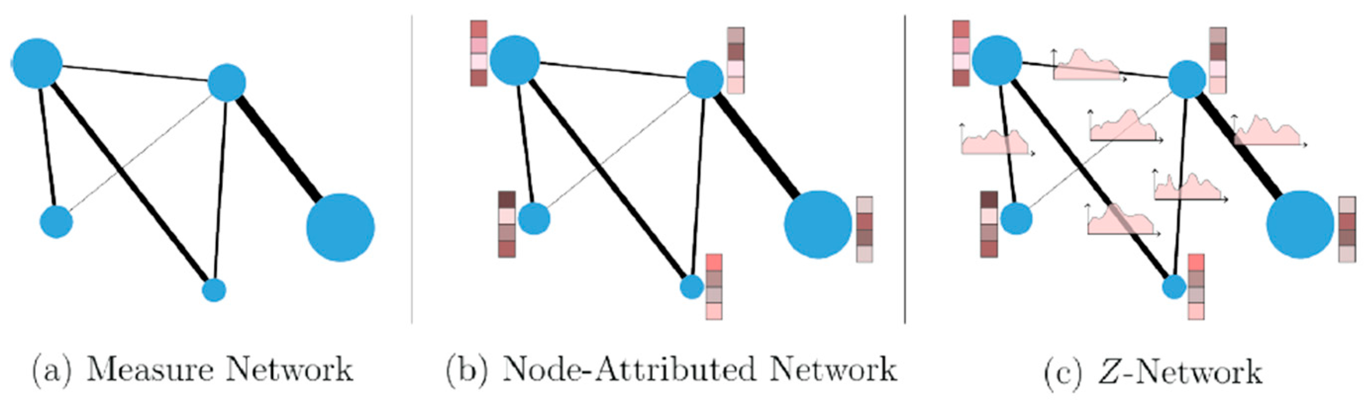
This paper is structured as follows: Section 2 reviews related work on network resilience. Section 3 presents networks as mm-spaces and their geometric and probabilistic properties. Distance metrics, including Hausdorff, Gromov–Hausdorff, Sturm, GW variants, and GW computational complexity, are covered in Section 4, providing the theoretical foundation for FUGW. Section 5 outlines the experimental design and data resources, and the computational results are explained in Section 6, with implications for resilience strategies being concluded. Finally, Section 7 presents the conclusions, discusses the limitations, and outlines future perspectives.

2. Related Work and Theoretical Foundations

Research on transportation network resilience has moved from topological measures toward distribution-based, geometry-aware frameworks. Early work in graph theory, such as betweenness centrality [2,12], highlighted structural bottlenecks but often ignored the dynamics of demand and temporal variability in usage. Recent reviews point out this gap, refs. [13,14] categorize resilience studies into purely structural or supply-demand models, and ref. [15] indicates that most resilience analyses are still limited to static networks and simplified disruption scenarios. Empirical work confirms that network design and demand loading both affect resilience [16].

In the transportation domain, numerous methods have been employed to assess vulnerability and resilience. Ref. [17] looked at network vulnerability models, emphasizing the need for metrics that integrate topological and operational factors. Ref. [18] proposed a step-by-step framework for resilience assessment, including recovery strategies, but they worked on simplified demand conditions. Ref. [19] looked at modeling techniques for different transportation types and approaches, finding that many network studies still focus on connectivity or redundancy and often ignore flow or time-based demand. Ref. [20] used the largest-connected-subgraph and efficiency drop metrics to quantify post-failure performance, but they do not take a formal distribution-based perspective. Current research on multilayer and interdependent transport networks also confirms that structural perturbations have cascading effects, but most studies still rely on graph metrics and network-flow simulations rather than metric-measure space comparisons [21]. Many vulnerability assessments describe travel times and structural disturbances without the aid of optimal transport tools [22]. In general, these systems, like designed infrastructure systems or even those in nature, can all be modeled using graphs; hence, a framework becomes available through which the systems’ structures and their dynamic characteristics can be analyzed [23,24,25].

By taking a graph-theoretic view, recent work has begun applying optimal transport (OT) and Wasserstein formulations to networked and transportation systems. While most OT-based studies were initially concerned with graph comparison, alignment, and shape matching [26,27,28,29], extensions of OT to network dynamics are emerging. Ref. [30] proposed Wasserstein attraction flows for dynamic mass transport on networks, tracking the evolution of node distributions with constrained barycenter updates according to network topology and capacity constraints.

This approach shows OT’s potential for network-level flow optimization but remains limited to balanced mass scenarios and does not directly quantify structural vulnerability or edge criticality. A key limitation of the Wasserstein distance is that it needs both measures to be in the same metric space [26], but in network vulnerability assessment, that is often not the case, because, for instance, removing edges changes the network’s intrinsic geometry.

The Gromov–Wasserstein (GW) distance overcomes this by comparing internal distance structures without needing a shared embedding [7,31]. Ref. [3] introduced a GW-based geometric framework for assessing structural vulnerability in urban transportation networks. By iteratively deleting edges and finding GW distances between the original and disrupted topologies, they identified critical links whose removal most alters network geometry. Their findings, especially the near-zero correlation between GW and betweenness centrality, show that GW captures global structural distortions overlooked by conventional graph-theoretic metrics. This work provides strong empirical evidence that OT-based distances can quantify systemic resilience in transportation systems. However, their application to transportation resilience—where disruptions create mass imbalance, dynamic demand, and topological alteration—remains scarce. This work provides strong empirical evidence that OT-based distances can quantify systemic resilience in transportation systems. However, their application to transportation resilience—where disruptions create mass imbalance, dynamic demand, and topological alteration—remains scarce.

In addition to these advances, the state of the art in unbalanced and Fused Optimal Transport (OT) in refs. [8,10] allows for the modeling of mass loss, demand variation, and feature integration, yet their direct application to network vulnerability assessment remains scarce. In this paper, we build upon these lines and apply Fused Gromov–Wasserstein (FUGW) to a temporally varying network, capturing diurnal congestion patterns and node demands across four periods (morning, noon, afternoon, night). This temporal dimension, combined with feature fusion and unbalanced regularization, provides a more comprehensive vulnerability analysis than prior approaches.

3. Distributional Definitions of Measure Metric Spaces

The analysis of network resilience under structural perturbations needs a representation that captures both the geometric organization of connections and the distributional heterogeneity of nodal attributes or demands. In this section, a network is viewed as a measure network space, integrating both its geometric structure and probabilistic distribution. This formulation presents a unified mathematical framework for comparing networks with differing topologies through their intrinsic relational geometry [7,24]. The following subsections progressively develop this idea—from metric spaces to measure network spaces—establishing the foundational hierarchy for the distributional framework underlying the Gromov–Wasserstein distance.

3.1. Metric Spaces

The metric space $(\mathit{X},{\mathit{d}}_{\mathit{X}})$ is a Polish metric space if and only if $\mathit{X}$ is a Polish space and the metric ${\mathit{d}}_{\mathit{X}}$ is one of the complete metrics compatible with the topology. A metric space is called Polish if it is separable and complete with respect to ${\mathit{d}}_{\mathit{X}}$, where $\mathit{X}$ is a set and ${\mathit{d}}_{\mathit{X}}:\mathit{X}\times \mathit{X}\to \mathbb{R}\ge 0$ is a function, called a metric, satisfying for all $\mathit{x},{\mathit{x}}^{\prime },{\mathit{x}}^{″}\in \mathit{X}$:

• $d_X\left(x,x^{\prime }\right)=0 \mathrm{i}\mathrm{f} \mathrm{a}\mathrm{n}\mathrm{d} \mathrm{o}\mathrm{n}\mathrm{l}\mathrm{y} \mathrm{i}\mathrm{f} x=x^{\prime };$
• $d_X(x,x^{\prime })=d_X(x^{\prime },x)$ (symmetry);
• $d_X(x,x^{″})\le d_X(x,x^{\prime })+d_X(x^{\prime },x^{″})$ (triangle inequality).

3.2. Metric Measure Spaces (mm-Spaces)

A measure metric space (mm-space) is a triple $\mathcal{X}=\left(\mathit{X},{\mathit{d}}_{\mathit{X}},\mathit{\mu }\right)$ with $\mathit{X}\subseteq {\mathbb{R}}^{{\mathit{h}}_{\mathit{x}}}$ not empty and a separable and completely metrizable space (i.e., $\mathit{X}$ is a Polish space), and ${\mathit{d}}_{\mathit{X}}:\mathit{X}\times \mathit{X}\to \mathbb{R}$ a (distance) metric generating the geometry of the space $\mathit{X}$ and $\mathit{\mu }\in {\mathcal{M}}^{+}$. The GW distance extends the OT framework to these spaces, allowing comparison between entire mm-spaces rather than between distributions. This generalization enables one to measure distances between shapes, graphs, and other structured objects whose elements are not directly aligned.

3.3. Measure Networks Spaces (m-Nets-Spaces)

The concept of a measure network generalizes that of a metric measure space by relaxing the requirement that the pairwise interaction function be a distance metric. This broadens the applicability of the GW framework to complex relational data structures. A measure network (or m-net) is a triple $\mathcal{X}=\left(\mathit{X},{\mathsf{\omega }}_{\mathbf{X}},\mathit{\mu }\right)$ where:

• $X$ is a separable and completely metrizable topological space (a Polish space);
• ${\mu }_X$ is a fully supported Borel probability measure on $X$;
• ${\omega }_X:X\times X\to R$ is a measurable function, called the network function.

The collection of all measure networks is denoted by $\mathcal{N}$. When ${\mathsf{\omega }}_{\mathbf{X}}$ satisfies the metric axioms and generates the topology of $\mathit{X}$, it is denoted ${\mathit{d}}_{\mathit{X}}$, and the corresponding triple ($\mathit{X},{\mathit{d}}_{\mathit{X}},\mathit{\mu }$) is a metric measure space belonging to the class $\mathcal{M}$. Measure networks include numerous important structures [32]:

• Pseudo-metric measure spaces.

A pseudo-metric ${\mathit{\omega }}_{\mathit{X}}:\mathit{X}\times \mathit{X}\to \mathit{R}$ satisfies all the metric axioms besides allowing ${\mathit{\omega }}_{\mathit{X}}(\mathit{x},{\mathit{x}}^{\prime })=0$ for $\mathit{x}\ne {\mathit{x}}^{\prime }$, which may occur for distinct points. Pseudo-metric measure spaces arise naturally as elements in the completion of $\mathcal{M}$ under Gromov–Wasserstein distances [33].

2.

Graphs as measure networks.

A finite graph $\mathit{G}=(\mathit{V},\mathit{E})$ can be viewed as an m-net by setting $\mathit{X}=\mathit{V}$, letting ${\mathit{\mu }}_{\mathit{X}}$ be the uniform measure, and defining the following [31]:

$${\mathit{\omega }}_{\mathit{X}}(\mathit{x},{\mathit{x}}^{\prime })=\left\{\begin{array}{cc}\mathbf{1}\hfill & \mathit{i}\mathit{f}\{\mathit{x},{\mathit{x}}^{\prime }\}\in \mathit{E}\\ \mathbf{0}\hfill & \mathit{o}\mathit{t}\mathit{h}\mathit{e}\mathit{r}\mathit{w}\mathit{i}\mathit{s}\mathit{e}\end{array}\right..$$

(1)

This provides a discrete example of an m-net.

3.

Generalized graph kernels.

More generally, one can define ${\omega }_X$ through other graph kernels, such as the graph Laplacian or a heat kernel [34].

The GW framework applies naturally to these generalized spaces. Indeed, it has become a key concept in the analysis of graphs and complex data representable as networks or relational structures, effectively extending optimal transport to settings where distributions cannot be compared pointwise [7].

3.4. Strong Isomorphism of Measure Networks

Structural equivalence between measure networks is captured through the notion of strong isomorphism. A measurable function $\mathit{\phi }:\mathit{X}\to \mathit{Y}$ between measure spaces $(\mathit{X},{\mathit{\mu }}_{\mathit{X}})$ and $(\mathit{Y},{\mathit{\mu }}_{\mathit{Y}})$ is measure-preserving if [32]:

$${\mathit{\phi }}_{\#}{\mathit{\mu }}_{\mathit{X}}\left(\mathit{A}\right)={\mathit{\mu }}_{\mathit{X}}\left({\mathit{\phi }}^{-1}\right(\mathit{A}\left)\right)={\mathit{\mu }}_{\mathit{Y}}\left(\mathit{A}\right)$$

(2)

for all measurable $A\subseteq Y$.

Let $X=\left(X,{\omega }_X,{\mu }_X\right)$ and $Y=\left(Y,{\omega }_Y,{\mu }_Y\right)$ be m-nets. A strong isomorphism from $X$ to $Y$ is a bijective, measure-preserving map $\phi :X\to Y$ with a measure-preserving inverse such that [32]:

$${\omega }_Y\left(\phi \right(x),\phi (x^{\prime }\left)\right)={\omega }_X\left(x,x^{\prime }\right) \forall (x,x^{\prime })\in X\times X$$

(3)

Strongly isomorphic measure networks are identical in both their measure-theoretic and structural properties.

3.5. Weak Isomorphism of Measure Networks

A weaker notion of equivalence, allowing for structural similarity up to measure-preserving transformations, is often sufficient in applications involving GW distances. Measure networks $\mathit{X}=\left(\mathit{X},{\mathit{\omega }}_{\mathit{X}},{\mathit{\mu }}_{\mathit{X}}\right)$ and $\mathit{Y}=\left(\mathit{Y},{\mathit{\omega }}_{\mathit{Y}},{\mathit{\mu }}_{\mathit{Y}}\right)$ are weakly isomorphic if there exists a Borel probability space $(\mathit{Z},{\mathit{\mu }}_{\mathit{Z}})$ and measure-preserving maps ${\mathit{\phi }}_{\mathit{X}}:\mathit{Z}\to \mathit{X}, {\mathit{a}\mathit{n}\mathit{d} \mathit{\phi }}_{\mathit{Y}}:\mathit{Z}\to \mathit{Y}$ such that [32]:

$${\mathit{\omega }}_{\mathit{X}}\left({\mathit{\phi }}_{\mathit{X}}\right(\mathit{z}),{\mathit{\phi }}_{\mathit{X}}({\mathit{z}}^{\prime }\left)\right)={\mathit{\omega }}_{\mathit{Y}}\left({\mathit{\phi }}_{\mathit{Y}}\right(\mathit{z}),{\mathit{\phi }}_{\mathit{Y}}({\mathit{z}}^{\prime }\left)\right)$$

(4)

for ${\mu }_Z\otimes {\mu }_Z$ almost every $(z,z^{\prime })\in Z\times Z$. Strong isomorphism implies weak isomorphism trivially. The converse holds for mm-spaces but not generally for arbitrary measure networks, since non-metric network functions can generate equivalence almost everywhere rather than pointwise.

3.6. Probabilistic Metric Spaces

In real-world applications, graph data can involve additional attributes in order to increase representation capability. For example, probabilistic metric spaces were first proposed by Menger in 1942 [35]; further discussion can be found in [36,37,38]. In other branches of graph data, such as molecular graphs described by [11], a molecular graph represents the structure of a molecule using nodes corresponding to atoms and edges corresponding to chemical bonds, where every node and edge can have categorical attributes that can then be transformed using one-hot representation to obtain node and edge representations in ${\mathbb{R}}^n$ and ${\mathbb{R}}^m$, where n and m represent the number of atom and bond types, respectively. Similarly, social networks frequently include attributed graphs where node attributes encode member statistics and edge attributes capture diverse interaction data, typically represented as non-binary values in Euclidean spaces. In such spaces, the notion of distance between two points is not represented by a single deterministic value but rather by a probability distribution over non-negative real numbers. Formally, a probabilistic metric space is a pair $(X,p_X)$, where for any two points $x,x^{\prime }\in X$, the “distance” $p_X(x,x^{\prime })$ is a Borel probability measure on ${\mathbb{R}}_{\ge 0}$ satisfying the following conditions:

• $x=x^{\prime }$ if and only if $p_X(x,x^{\prime })={\delta }_0$;
• $p_X(x,x^{\prime })=p_X(x^{\prime },x)$ for all $x,x^{\prime }\in X$;
• For all $x,x^{\prime },x^{″}\in X$ and all $s,t\in {\mathbb{R}}_{\ge 0}$, $min\left(p_X\right(x,x^{\prime }\left)\right(0,s],\hspace{0.17em}{p}_X(x^{\prime },x^{″}\left)\right(0,t\left]\right)\le p_X(x,x^{″})(0,s+t]$.

The third axiom generalizes the classical triangle inequality. When distances are deterministic, that is, $p_X(x,x^{\prime })={\delta }_{d_X\left(x,x^{\prime }\right)}$ for some metric $d_X$ on X, these axioms reduce to the standard metric axioms, with the third condition equivalent to the triangle inequality for $d_X$. Under this formulation, probabilistic metric spaces naturally become Z-networks [39].

3.7. Attributed Network in m-Nets-Spaces

The analysis of network structures can be categorized based on the types of data associated with their nodes and edges. A basic representation is a graph with edge weights and node weights, visualized through size variations, which is encoded as a measure network and compared using the GW distance [26]. A more complex structure considers a weighted graph with additional node features, where each node is assigned a vector in ${\mathbb{R}}^n$, which makes it possible to compare them via the Fused Gromov–Wasserstein (FGW) distance [29]. Furthermore, graphs can be enriched with edge features, assigning a point in a fixed metric space $Z$ to each edge—such as a one-dimensional probability distribution or time-varying distance in this case—modeled as $Z$-networks, allowing comparison through a proposed distance tailored to the chosen target space $Z$. In the context of this study, the transportation network derived from benchmark data incorporates node demands as features, aligning them partially with the second network in Figure 1, specifically with the inclusion of four time periods (morning, noon, afternoon, night) with dynamically adjusted edge distances to simulate diurnal congestion, which introduces a temporal edge feature. It is a kind of probabilistic network. Graphs with attributes in more exotic metric spaces are also relevant, with detailed examples provided by [40,41]. Building on this, Yang et al. [42] apply a general model for graphs with metric space-attributed nodes and edges, which we adapt to our study. In this framework, an attributed network is defined by a set of hyperparameters $H=(p,\Omega ,d_{\Omega },\Psi ,d_{\Psi })$, where $p\in [1,\infty ]$ and $(\Omega ,d_{\Omega })$, $(\Psi ,d_{\Psi })$ are separable metric spaces. An H-network is a five-tuple $(X,{\psi }_X,{\varphi }_X,{\omega }_X,{\mu }_X)$ that forms a measure network with ${\varphi }_X\in L^p({\mu }_X\otimes {\mu }_X$) modeling the graph structure, ${\psi }_X\in L^p(X,{\mu }_X;\Psi )$ represents node features in $\Psi$, and ${\omega }_X\in L^p(X\times X,{\mu }_X\otimes {\mu }_X;\Omega )$ models edge features in $\Omega$.

4. Distances Between Measure Network Space (m-Net-Space)

Building upon the formalization of networks as measuring network spaces in Section 2, in the current section, quantitative methods will be developed to compare these spaces. Having defined the geometric, measure-theoretic, and relational foundations of networks, we now turn to distance functionals that capture similarities and differences between them. These distances extend classical geometric notions—such as the Hausdorff distance—to measure metric and measure network settings, thereby integrating both spatial and distributional aspects. We begin with the Hausdorff distance for subsets within a fixed space and progress to more general constructions including the Wasserstein distances, Gromov–Hausdorff, Sturm, and Gromov–Wasserstein distances, as well as their fused and unbalanced variants, which are central to modern optimal transport-based network analysis.

4.1. Wasserstein Distance

The Wasserstein distance is a cornerstone of optimal transport theory and takes a pivotal role in modern statistics, machine learning, and computational geometry. It offers a practical discrepancy measure between probability distributions by incorporating the underlying geometry of the sample space, which has been recently applied in the distributionally robust optimization setting [43]. Unlike information-theoretic divergences such as the Kullback–Leibler or total variation distances, the Wasserstein distance satisfies the axioms of a metric and reflects the spatial arrangement of mass within the distributions [44,45].

In many computational and applied contexts, the measures $\mu$ and $\nu$ are discrete and supported on finite sets:

$$\mu ={\sum }_{i=1}^n{\mu }_i{\delta }_{x_i}, \nu ={\sum }_{j=1}^n{\nu }_j{\delta }_{y_j}$$

(5)

In the discrete setting, the p-Wasserstein distance becomes a finite-dimensional linear optimization problem:

$$W_p^p(\mu ,\nu )=\underset{P\in U(\mu ,\nu )}{\min }\sum _{i=1}^n\sum _{j=1}^m{d}^p\left(x_i,y_j\right)P_{ij}$$

(6)

where:

• $P=P_{ij}$ is a transport matrix (or coupling matrix) indicating how much mass is moved from $x_i$ to $y_j$;
• $U(\mu ,\nu )$ is the transport polytope:

$$U(\mu ,\nu )=\{P\in {\mathbb{R}}_{+}^{n\times m}:{\sum }_j{P}_{ij}={\mu }_i,{\sum }_i{P}_{ij}={\nu }_j\}$$

(7)

Each feasible matrix $P\in U(\mu ,\nu )$ defines a valid mass-transport plan that preserves the marginals. The objective function measures the total transport cost under the ground distance $d\left(x_i,y_j\right)$.

When the transport plan is restricted to deterministic assignments, i.e., $P_{ij}\in \left\{\mathrm{0,1}\right\}$ with one non-zero entry per row (and per column, for uniform measures), the problem reduces to the Monge formulation of discrete optimal transport.

4.2. Hausdorff Distance

The Hausdorff distance is a classical tool in geometry and analysis for comparing two subsets of a metric space. Given a metric space $(Z,d_Z)$, the Hausdorff distance between two non-empty subsets $A,B\subset Z$ determines how far the sets are from matching one another. It is defined as the largest distance one has to travel from a point in one set to reach the other set. Intuitively, if every point of $A$ is close to some point of $B$, and vice versa, the Hausdorff distance is small; otherwise, it is large.

Formally, the Hausdorff distances are defined as follows [46]:

$${\mathcal{H}}_Z(A,B)\stackrel{\scriptscriptstyle\mathrm{def}}{=}\left(\underset{a\in A}{\sup } \underset{b\in B}{\inf } d_Z\left(a,b\right),\underset{b\in B}{\sup } \underset{a\in A}{\inf } d_Z(a,b)\right).$$

(8)

This construction turns the family of compact subsets $\mathcal{K}\left(Z\right)$ of $Z$ into a metric space. A fundamental property is that if the underlying space $Z$ is compact, the metric space $\left(\mathcal{K}\right(Z),H_Z)$ is also compact (see e.g., [47,48]). This makes the Hausdorff distance particularly valuable in geometric analysis, shape comparison, and computer vision, where compact sets such as curves, surfaces, or finite point clouds are often studied. 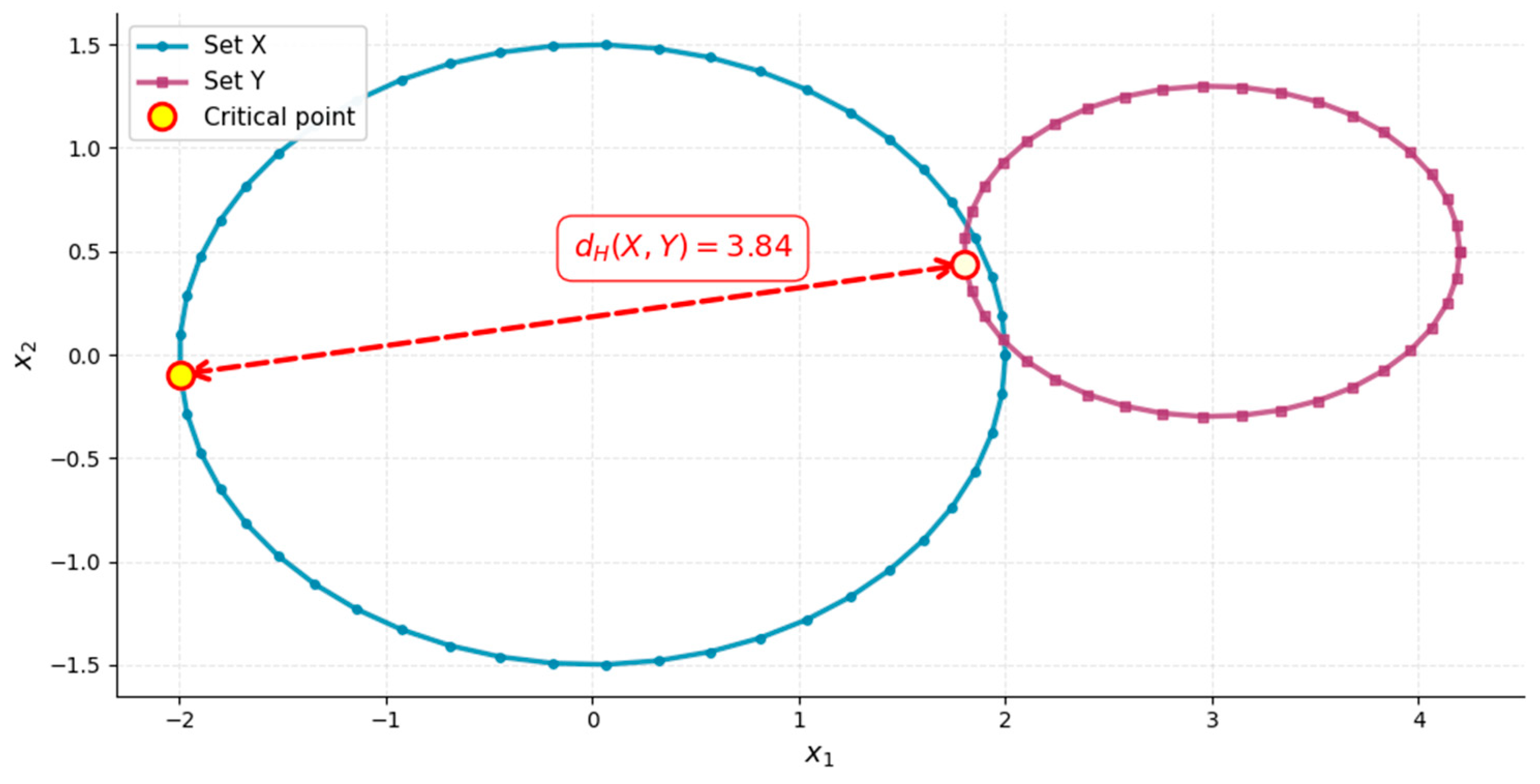Figure 2 shows the computation of the Hausdorff distance in ${\mathbb{R}}^2$, where the distance matches the largest minimal distance between the boundary points of the two sets.

The Hausdorff distance also admits an interpretation that parallels the theory of optimal transport, especially to Wasserstein distances, which are defined between probability measures. Following [7], one can interpret Wasserstein distances as acting on weighted sets (measures), while the Hausdorff distance corresponds to comparing the underlying unweighted supports.

$$\mathcal{R}(A,B)\stackrel{\scriptscriptstyle\mathrm{def}}{=}\left\{R\in \mathcal{X}\times \mathcal{Y}:\begin{array}{c}\forall a\in A, \exists b\in B such that \left(a,b\right)\in R,\\ \forall b\in B, \exists a\in A such that \left(a,b\right)\in R\end{array}\right\}$$

(9)

Formally, in the Kantorovich formulation of optimal transport, one seeks couplings between probability measures $\alpha$ and $\beta$. Replacing couplings of measures with couplings of sets and replacing integration with maximization (since we are no longer averaging weights), one obtains a definition that coincides with the Hausdorff distance.

$${\mathcal{H}}_Z(A,B)=\underset{R\in \mathcal{R}\left(A,B\right)}{\inf }\underset{(a,b)\in R}{\sup }d(a,b).$$

(10)

This connection is particularly strong with the $\infty$-Wasserstein distance. Indeed, for any probability measures $(\alpha ,\beta )$ supported on sets $A,B\subset Z$, one has the following:

$$\mathcal{H}(A,B)\le W_{\infty } (\alpha , \beta )$$

(11)

where the support of an optimal coupling $\pi \in \mathcal{U}(\alpha ,\beta )$ provides a natural set coupling between A and B [6]. The Hausdorff distance is widely used in applications where the geometry of sets must be compared.

4.3. Gromov–Hausdorff

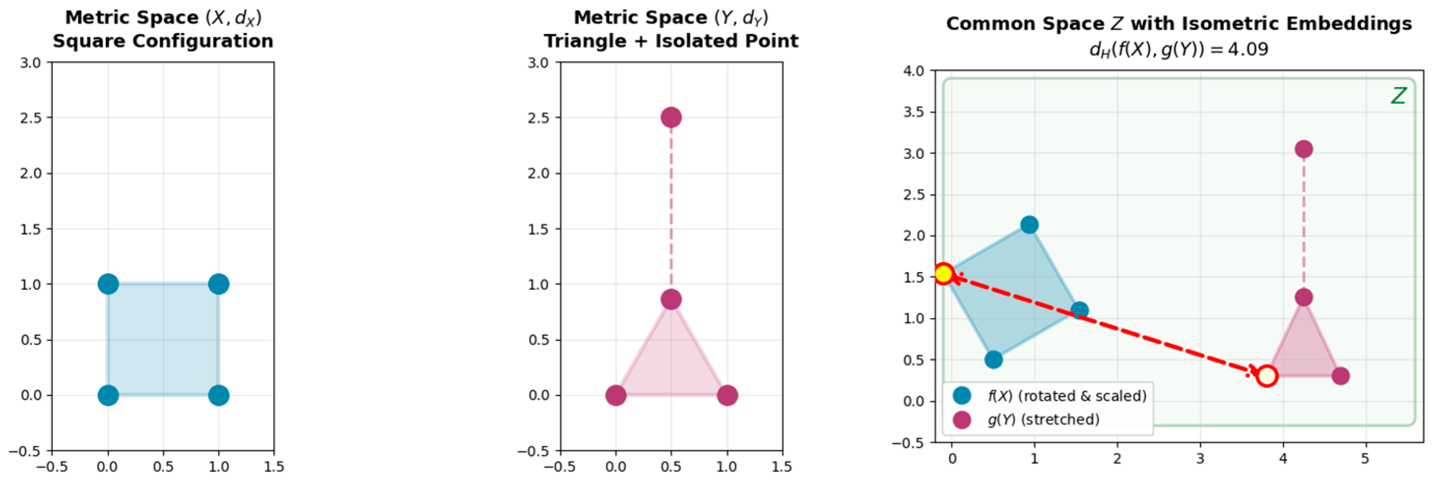
The Gromov–Hausdorff (GH) distance [49,50] extends the Hausdorff distance from subsets of a fixed metric space to the comparison of entire metric spaces. While the Hausdorff distance quantifies how far two subsets of the same space are from coinciding, the GH distance measures how far two metric spaces $(X, d_X)$ and $(Y, d_Y)$ are from being isometric, i.e., structurally identical as metric spaces. Formally, the idea is to embed both spaces into a common metric space $(Z,d_Z)$ using isometric embeddings, $f:X\to Z$ and $g:Y\to Z$, and then compute the Hausdorff distance between the images $f\left(X\right)$ and $g\left(Y\right)$ (see Figure 3). It is defined as the minimum Hausdorff distance between every possible isometric embedding of the two spaces in a third one [46]:

$$d_{GH}\left(d_X,d_Y\right)\stackrel{\scriptscriptstyle\mathrm{def}}{=}\underset{Z,f,g}{\inf }\left({\mathcal{H}}_Z\right(f\left(X\right),g\left(Y\right)): f:X\stackrel{isom}{\to }Z, g:Y\stackrel{isom}{\to }Z$$

(12)

where the infimum is taken over all possible choices of common metric spaces Z and all isometric embeddings $f,g$. By construction, the constraint on embeddings guarantees that the original distances are preserved:

$d_Z\left(f\left(x\right), f\left(\acute{x}\right)\right)= d_X \left(x,\acute{x}\right)for any \left(x,\acute{x}\right)\in X\times X$ and similarly for g.

This definition implies that GH defines a distance between compact metric spaces up to isometries, so that in particular $d_{GH}(d_X , d_Y) = 0$ if and only if there exists an isometry $h : X ⟶ Y$, i.e., h is bijective and $d_Y\left(h\right(x), h(\acute{x}\left)\right) = d_X (x, \acute{x})$ for any $(x,\acute{x})\in X\times X$.

Following [7], the GH distance can be reformulated using couplings between the two spaces, similar in spirit to the optimal transport approach as follows:

$$\begin{gathered} d_{GH}\left(d_X,d_Y\right) \\ ={\displaystyle \frac{1}{2}}\underset{R\in \mathcal{R}(X,Y)}{\inf }\underset{\left(\right(x,y),\left(\acute{x},\acute{y}\right))\in R^2}{\sup }\left|d_X \left(x, \acute{x}\right)-d_Y \left(y, \acute{y}\right)\right|. \end{gathered}$$

(13)

For discrete spaces $X = {\left(x_i\right)}_{i =1}^n,Y = {\left(y_j\right)}_{j=1}^m$ represented using a distance matrix $\mathit{D}= {\left(d_X \left(x_i, x_{\acute{i}}\right)\right)}_{i,\acute{i} }\in {\mathbb{R}}^{n\times n}, \acute{\mathit{D}}= {\left(d_Y\left(y_j , y_{\acute{j}}\right)\right)}_{j,\acute{j}} \in {\mathbb{R}}^{m\times m}$, one can rewrite this optimization using binary matrices $\mathit{R}\in {\{0, 1\}}^{n\times m}$ indicating the support of the set couplings R as follows:

$$d_{GH}\left(D,D^{\prime }\right)={\displaystyle \frac{1}{2}}\underset{R1>0,R^{T}1>0}{\inf }\underset{i,i^{\prime },j,j^{\prime }}{\max }{R}_{i,j}{R}_{\acute{i,\stackrel{´}{j}}}\left|D_{i,i^{\prime }}-\acute{D_{j,j^{\prime }}}\right|.$$

(14)

The initial motivation of the GH distance is to define and study the limits of metric spaces, as illustrated in Figure 4, and we refer to [48] for details. There is an explicit description of the geodesics for the GH distance [51].

4.4. Sturm

Sturm’s distance [52] combines ideas of the Gromov–Hausdorff distance [7,53] with OT.

It consists in mapping two mm-spaces $\mathcal{X}=\left(X,d_X,\mu \right)$ and $\mathcal{Y}=\left(X,d_Y,\nu \right)$ isometrically into a third space $\left(Z,d_Z\right)$, and performing OT on that third space. It reads as follows:

$$\begin{gathered} d_{Sturm}\left(X,Y\right) \\ \triangleq \underset{\left(Z,d_Z\right),\mathit{\psi X},\mathit{\psi Y}}{\mathrm{Inf}}{H}_{d_Z}({\left({\psi }_X\right)}_{\#}\mu ,{\left({\psi }_Y\right)}_{\#}\nu ), \end{gathered}$$

(15)

where $d_Z$ is the ground OT cost on $Z, {\psi }_X:X\to Z and {\psi }_Y:Y\to Z$ are isometrically embedded into Z. By comparison, the Gromov–Hausdorff distance between two metric spaces reads as follows:

$$\begin{gathered} GH\left(\left(X,d_X\right),\left(Y,d_Y\right)\right) \\ \triangleq \underset{\left(Z,d_Z\right),{\psi }_X,{\psi }_Y}{\mathrm{Inf}}{H}_{d_Z}\left({\psi }_X\right(X),{\psi }_Y(Y\left)\right) \end{gathered}$$

(16)

where $\left(Z,d_Z\right),{\psi }_X,{\psi }_Y$ satisfy the same constraints as for $d_{Sturm}$, and $H_{d_Z}(X,Y)$ is the Hausdorff distance between two sets $X,Y\subset Z$ and reads as follows:

$$\begin{gathered} H_{d_Z}\left(X,Y\right) \\ \triangleq max\{\underset{x\in X}{\mathit{sup}}\underset{y\in Y}{\mathit{inf}}{d}_Z(x,y),\underset{y\in Y}{\mathit{sup}}\underset{x\in X}{\mathit{inf}}{d}_Z(x,y)\}. \end{gathered}$$

(17)

A fundamental difference between Sturm’s distance and the Gromov–Hausdorff distance is the extra information contained in the measure. It allows defining integrals on $\mathcal{X}$ and $\mathcal{Y}$, which are smoother quantities than the suprema/infima used for the Gromov–Hausdorff distance.

Sturm’s distance was motivated by theoretical considerations, namely comparing the curvature of spaces. Unfortunately, it is difficult to implement exactly and efficiently, since a triangle inequality constraint on $d_Z$ as well as an isometry constraint on the maps (${\psi }_X,{\psi }_Y$) must be imposed. Furthermore, OT is concave w.r.t. to the input cost $d_Z$; thus, the minimization in $d_Z$ yields a non-convex problem. This is the reason why we consider another distance between mm-spaces, which is more amenable to computations.

4.5. Gromov–Wasserstein

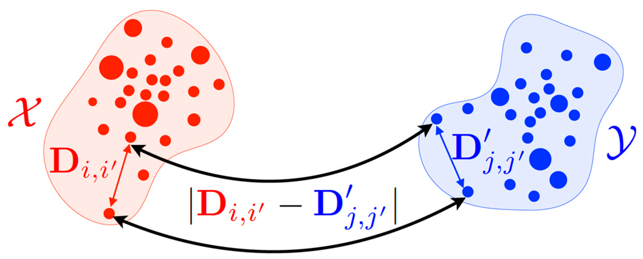
Optimal Transport enables computing assignments (or permutations) that account for metric similarities between samples. However, such a metric may not exist when the measures are defined on two different spaces. GW aims to define a meaningful distance between two mm-spaces, $\mathcal{X}$ and $\mathcal{Y}$, each represented as a probability measure over their elements and attributes. The GW distance is a strong generalization of the classic Wasserstein distance. It solves a key problem: comparing distributions that are not in the same space. The standard Wasserstein distance W₂ needs both distributions in a common space to compute direct pairwise distances. Gromov–Wasserstein, however, compares distributions using their internal structural relationships. It extends optimal transport to cases where distributions cannot be compared point by point [7]. Instead of computing distances between individual samples from two distributions, GW realigns the metric spaces by comparing their internal distance structures through a transport between distance matrices. Let $\mathcal{X}=(X,d_X,\mu )={\left\{\right(x_i,d_X(x_i,x_k),a_i\left)\right\}}_{i=1}^n$ and $\mathcal{Y}=(Y,d_Y,\nu )={\left\{\right(y_j,d_Y(y_j,y_l),b_j\left)\right\}}_{j=1}^m$ be two finite metric measure spaces with weight vectors $a\in {\Delta }_n,b\in {\Delta }_m$. Denote by $D^X\in {\mathbb{R}}^{n\times n}$ and $D^Y\in R^{m\times m}$ their pairwise distance (or cost) matrices, $D_{i,k}^X=d_X(x_i,x_k)$ and $D_{j,l}^Y=d_Y(y_j,y_l)$. The GW distance is designed to compare structured mm-spaces, without requiring any embedding in a common ambient space.

The (quadratic) Gromov–Wasserstein problem for a generic loss $L:\mathbb{R}\times \mathbb{R}\to {\mathbb{R}}^{+}$ is written in the discrete setting as follows:

$$G{W}_2\left(\mu ,\nu \right)=\underset{P\in U(a,b)}{\min }\sum _{\begin{array}{c}0\le i,k<n\\ 0\le j,l<m\end{array}}L(D_{i,k}^X, D_{j,l}^Y)P_{i,j}{P}_{k,l}$$

(18)

where $P$ belongs to the transportation polytope:

$$U(a,b)=\{P\in {\mathbb{R}}_{+}^{n\times m}:P{1}_m=a,P^{\top }{1}_n=b\}$$

(19)

A common and practical choice for the loss is the squared difference $L(a,b)={(a-b)}^2$, which yields the standard squared GW objective used in most algorithmic papers. The objective in (GW) is a quadratic form in the coupling P and is equivalent, in the balanced n = m case, to a Quadratic Assignment Problem (QAP). The QAP formulation exposes the non-convex and combinatorial character of GW in its discrete form. This discrete quadratic structure is the root of the computational hardness of exact GW [7].

GW compares the internal metric structure of $X$ and $Y$, by measuring how well the pairwise distances in $\mathcal{X}$ match those in $\mathcal{Y}$ under the coupling P. Unlike classical optimal transport, GW distance does not require the nodes to live in a common feature space (Figure 4).

4.5.1. Unbalanced Gromov–Wasserstein

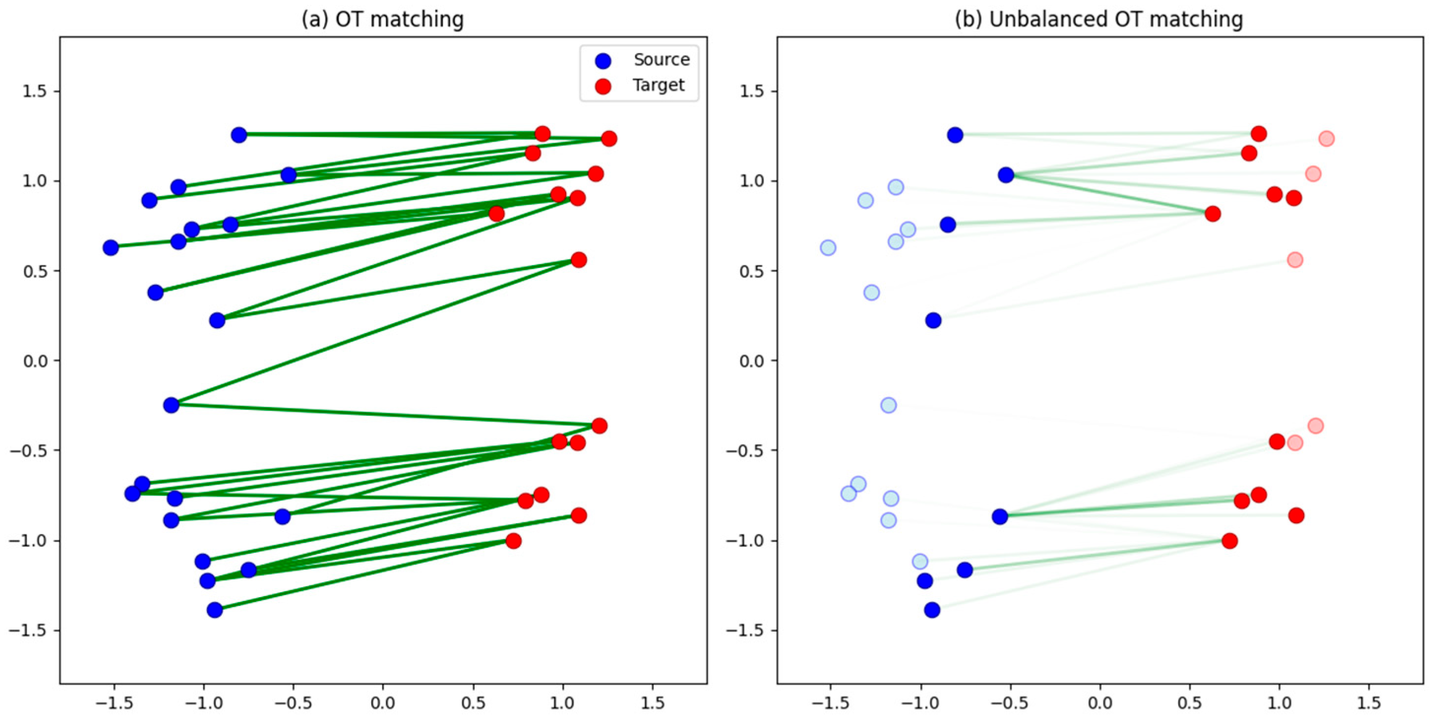
The Unbalanced Gromov–Wasserstein (UGW) divergence constitutes the computationally tractable core of the unbalanced optimal transport (UOT) framework [27]. Figure 5 illustrates a motivating example contrasting optimal transport (OT) and UOT matchings between two point clouds. In the balanced OT case (Figure 5a), every point from the source distribution must be matched to some point in the target distribution, even when certain regions or “modes’’ of the data are distant or unmatched, leading to unrealistic correspondences. In contrast, the unbalanced formulation (Figure 5b) allows portions of mass to be discarded, effectively ignoring outlier samples and yielding a more meaningful correspondence between comparable regions. This capacity to handle differing support motivates the introduction of UGW divergence.

It is designed to preserve the geometric interpretability of the classical GW distance while enabling flexibility in cases where the total transported mass between source and target distributions differs. This relaxation is crucial for practical applications—such as transportation or communication network analysis as will be shown in Section 6—where disruptions, congestion, or demand fluctuations can alter the effective mass distribution across nodes or edges. In such settings, the UGW divergence naturally models partial correspondence between baseline and perturbed network states, allowing critical structural changes to be quantified even when total flow or demand is not conserved.

The divergence builds upon a natural extension of the classical formulation. While the original Gromov–Wasserstein distance enforces strict marginal constraints $P_1=\mu$ and $P_2=\nu$, which implies perfect conservation of mass, the UGW divergence relaxes these constraints through the introduction of penalty terms that allow for controlled mass creation and destruction. This relaxation enables a soft correspondence between domains that differ in size, shape, or density, without requiring one-to-one matching of all elements. This could be the place to start determining the difference between $n \ne m$.

Formally, given two measure network spaces $\mathcal{X}=(X, {\omega }_X, \mu )$ and $\mathcal{Y}=(Y,{\omega }_Y,\nu )$, the UGW divergence is defined as follows:

$$\underset{P}{\min }\stackrel{Gromov-Wasserstein loss L_{GW}\left(P\right)}{\overbrace{\sum _{\begin{array}{c}0\le i,k<n\\ 0\le j,l<p\end{array}}{\left|D_{i,k}^X- D_{j,l}^Y \right|}^2{P}_{i,j}{P}_{k,l}}}+\rho \stackrel{Marginal constraints L_U\left(P\right)}{\overbrace{\left(KL\right(P_{\#1} \otimes P_{\#1}|w^X \otimes w^X)+KL(P_{\#2} \otimes P_{\#2}|w^Y \otimes w^Y)}}+\stackrel{Entropy }{\overbrace{\epsilon E\left(P\right)}}$$

(20)

where:

• $D_{i,k}^X$: pairwise distance between nodes i and k in the source space (baseline network);
• $D_{j,l}^Y$: pairwise distance between nodes j and l in the target space (modified network);
• P: transport plan (coupling matrix between source and target nodes);
• $w^X$: probability distribution (weights) over source samples/nodes;
• $w^Y$: probability distribution over target samples/nodes;
• $KL(P_{\#1} \otimes P_{\#1}|w^X \otimes w^X)$ penalizes deviation of the source marginal of P (denoted $P_{\#1}$) from $w^X$;
• $KL(P_{\#2} \otimes P_{\#2}|w^Y \otimes w^Y)$ penalizes deviation of the target marginal of P (denoted $P_{\#2}$) from $w^Y$;
• $\rho$ controls the strength of marginal relaxation, i.e., how strictly the transport plan must respect the input distributions;
• $\epsilon$: entropic regularization parameter.

$L_{GW}\left(P\right)$ penalizes changes in geometry, and $L_U\left(P\right)$ fosters matching all parts of the source and target distributions. Equation (20) refers to relaxing the hard marginal constraints of the underlying OT problem into soft ones as unbalancing. Here, $P_{\#1} \triangleq {\left({\sum }_j{P}_{i,j}\right)}_{0\le i<n}$ denotes the first marginal distribution of P, and $P_{\#2} \triangleq {\left( {\sum }_i{P}_{i,j}\right)}_{0\le j<p}$ is the second marginal distribution of P. The notation ⊗ represents the Kronecker product between two vectors or two matrices. $KL(·|·)$ denotes the Kullback–Leibler divergence, which is a typical choice to measure the discrepancy between two measures in the context of unbalanced optimal transport [54]. The last term $E\left(P\right)\triangleq KL (P \otimes P|(w^s \otimes w^t)\otimes \left(w^s\otimes w^t\right))$ is mainly introduced for computational purposes, as it helps accelerate the approximation scheme of the optimization problem. Typically, it is used in combination with a small value of $\epsilon$, so that the impact of other terms is not diluted.

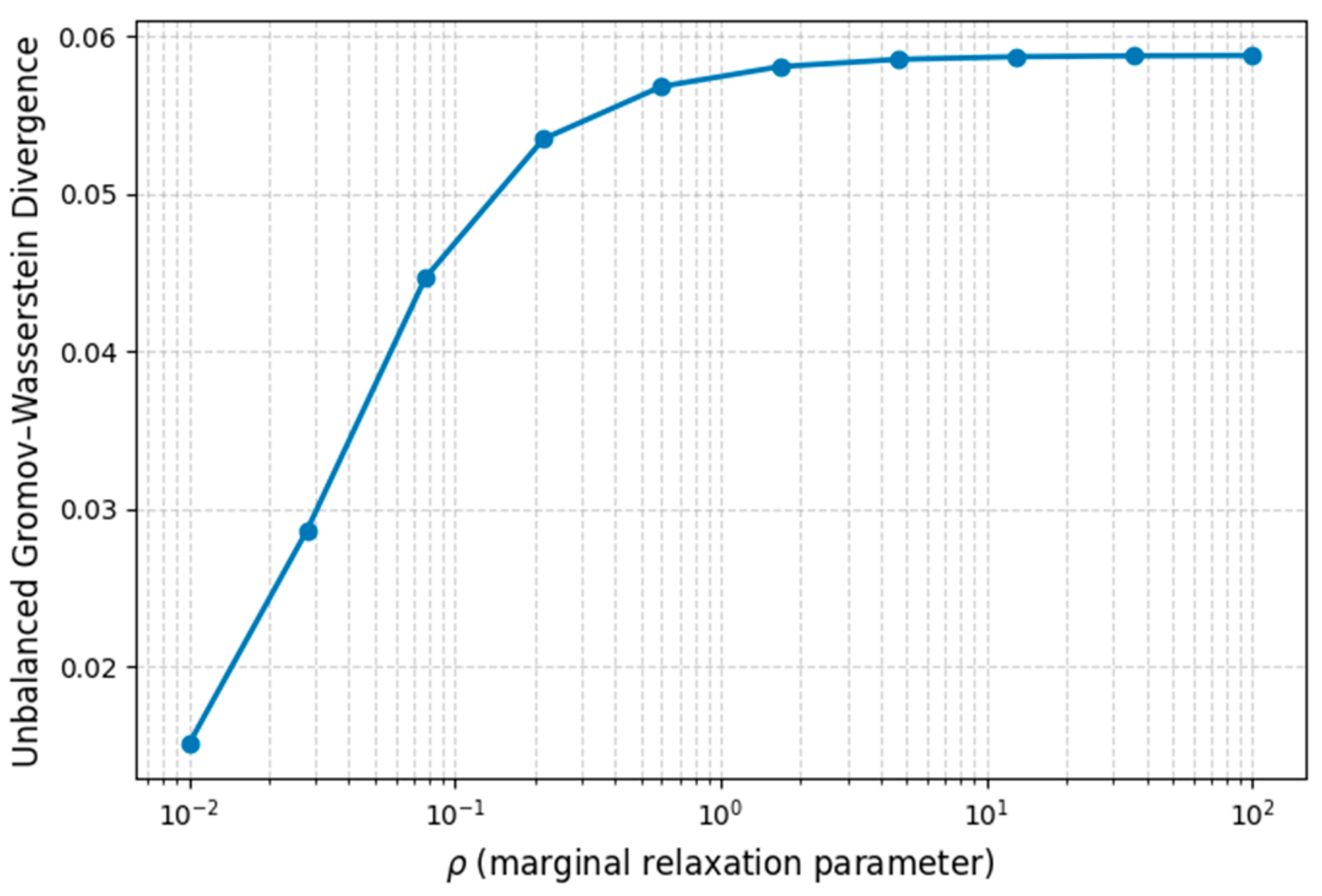
Figure 6 demonstrates how the marginal relaxation parameter ρ controls the balance between mass preservation and geometric alignment in UGW transport for two synthetic metric spaces: a circular arrangement of eight nodes and an elliptical arrangement of six nodes. At low ρ values ($\rho < 0.1$), weak marginal constraints permit mass creation/destruction to accommodate the unequal cardinalities, yielding lower divergence as the algorithm prioritizes structural matching. The divergence rises sharply between $0.1 < \rho < 1$ as marginal penalty strengthens and then plateaus for $\rho > 1$, converging to the balanced Gromov–Wasserstein regime where mass conservation is strictly enforced despite the dimension mismatch. 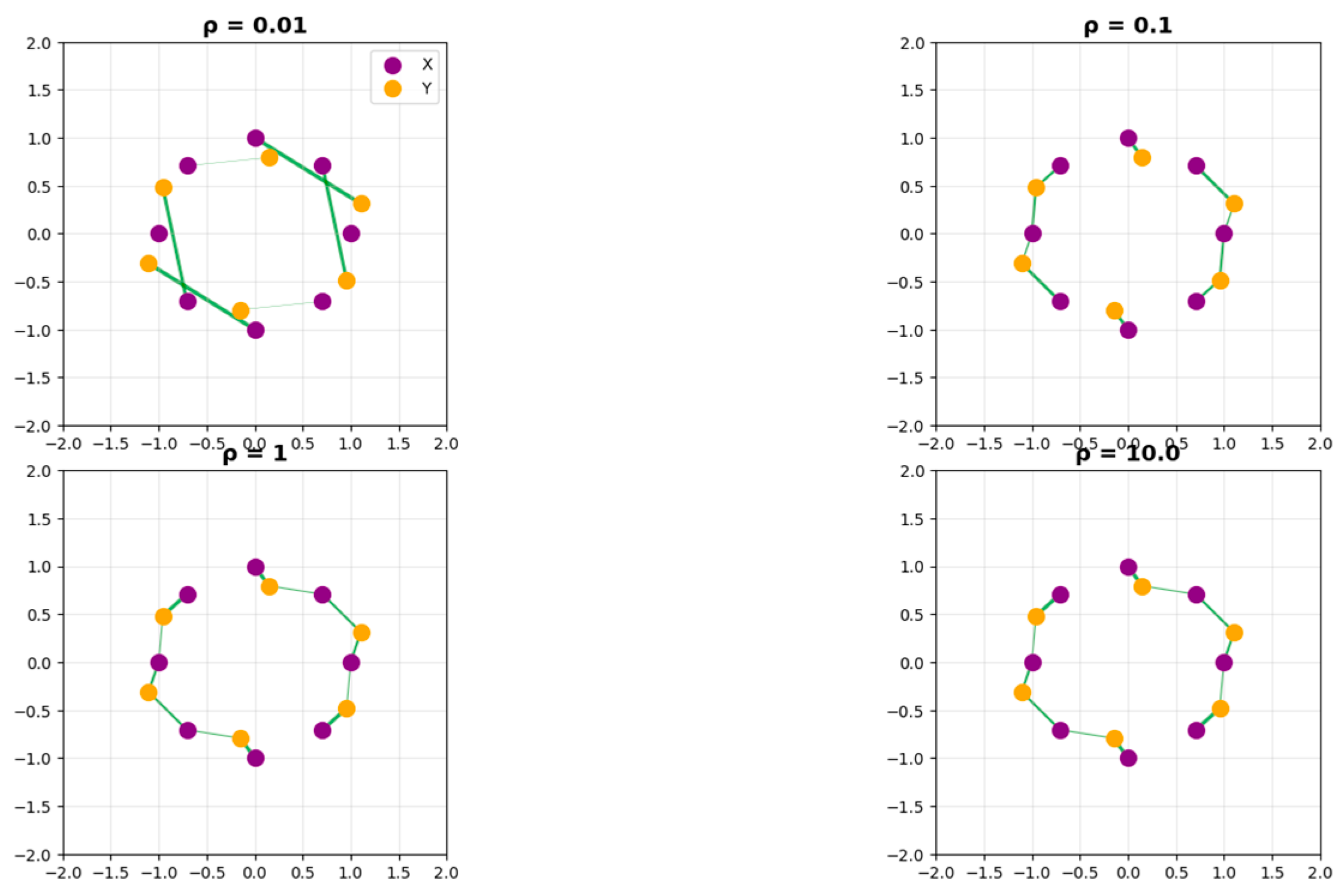Figure 7 visualizes the corresponding transport plans, where the line thickness between source (purple) and target (orange) nodes represents the transported mass. At $\rho = 0.01$, the transport is highly diffuse with many weak connections, reflecting flexible mass redistribution. As ρ increases to 0.1 and 1.0, the connections become more concentrated and structured, with clearer one-to-many matchings emerging. This transition illustrates how ρ selection is critical: small values enable flexible partial matching between spaces of different sizes, while large values recover classical balanced transport with near-deterministic assignments.

4.5.2. Fused Unbalanced Gromov–Wasserstein

The Fused Unbalanced Gromov–Wasserstein (FUGW) divergence extends the UGW framework by jointly accounting for feature similarity and geometric correspondence [10]. This fusion enables a more comprehensive alignment of structured data—such as cortical surfaces or functional networks—where both intrinsic geometry and node-level attributes carry meaningful information. The FUGW divergence is especially suitable for transportation networks. Compared to UGW, FUGW adds a fusion mechanism that balances structural and feature-based comparisons, making it sensitive to edges that are both topologically central and functionally critical. This sensitivity is crucial for transportation networks, where disruptions may create minor topological changes but major demand redistribution or vice versa. By integrating geometry, features, and unbalanced measures, FUGW delivers a robust, interpretable, and comprehensive framework for identifying edges whose failure would most compromise network vulnerability.

Let $F^X\in {\mathbb{R}}^{n,c}$ denote the feature matrix of the source domain, where each row $F_i^X$ encodes a c-dimensional feature vector (e.g., functional activation values) associated with vertex i. In this study, $F^X$ encodes node demands across four temporal periods, yielding c = 4 dimensional feature vectors. The corresponding pairwise distance matrix and vertex weights are given by $D_X \in {\mathbb{R}}_{n,n}^{+}$ and $w_X \in {\mathbb{R}}_n^{+}$, respectively. Analogously, the target domain is represented by $F^Y \in R^{m,c}$, $D^t \in {\mathbb{R}}_{+}^{m,m}$, and $w^Y \in {\mathbb{R}}_{+}^m$. In the absence of prior information, uniform vertex weights are adopted:

$$w^X \triangleq ({\displaystyle \frac{1}{n}},..., {\displaystyle \frac{1}{n}}), w^Y \triangleq ({\displaystyle \frac{1}{m}},...,{\displaystyle \frac{1}{m}})$$

(21)

Given the hyperparameter tuple $\theta \triangleq (\rho ,\alpha ,\epsilon )$, where $\rho ,\epsilon \in R_{+}$ and $\alpha \in \left[\mathrm{0,1}\right]$, the FUGW loss for a transport plan $P \in {\mathbb{R}}^{n,p}$ is defined as follows:

$$\begin{gathered} L_{\theta }(P) \triangleq (1-\alpha )\stackrel{Wasserstein loss L_W\left(P\right)}{\overbrace{\sum _{\begin{array}{c}0\le i<n\\ 0\le j<p\end{array}}{\left|\right|F_i^X- F_j^Y \left|\right|}_2^2 P_{i,j}}}+ \alpha \stackrel{Gromov-Wasserstein loss L_{GW}\left(P\right)}{\overbrace{\sum _{\begin{array}{c}0\le i,k<n\\ 0\le j,l<p\end{array}}{\left|D_{i,k}^X- D_{j,l}^Y \right|}^2{P}_{i,j}{P}_{k,l}}} \\ +\rho \stackrel{Marginal constraints L_U\left(P\right)}{\overbrace{\left(KL\right(P_{\#1} \otimes P_{\#1}|w^X \otimes w^X)+KL(P_{\#2} \otimes P_{\#2}|w^Y \otimes w^Y)}} +\stackrel{Entropy }{\overbrace{\epsilon E\left(P\right)}} \end{gathered}$$

(22)

• When $\alpha = 0$, the divergence reduces to pure UGW, focusing only on structural changes;
• When $\alpha = 1$, only node attributes are considered;
• Intermediate values yield a fused metric, capturing both topological disruption and shifts in demand.

The final objective seeks the optimal coupling $P^{*}$ minimizing this loss:

$$FUGW\left(X^X,X^Y\right) \triangleq \underset{P\ge 0}{\inf }{L}_{\theta }\left(P\right)$$

(23)

where $X^X \triangleq \left(F^X,D^X,w^X\right)$ and $X^Y \triangleq \left(F^Y,D^Y,w^Y\right)$.

The term $L_W\left(P\right)$ aligns vertices with similar feature profiles, while $L_{GW}\left(P\right)$ enforces geometric consistency between the source and target domains. The unbalanced regularization $L_U\left(P\right)$ promotes soft marginal matching, thereby accommodating local mass discrepancies. The entropy term $E\left(P\right)$ ensures smoothness of the coupling and improves the stability of iterative optimization schemes.

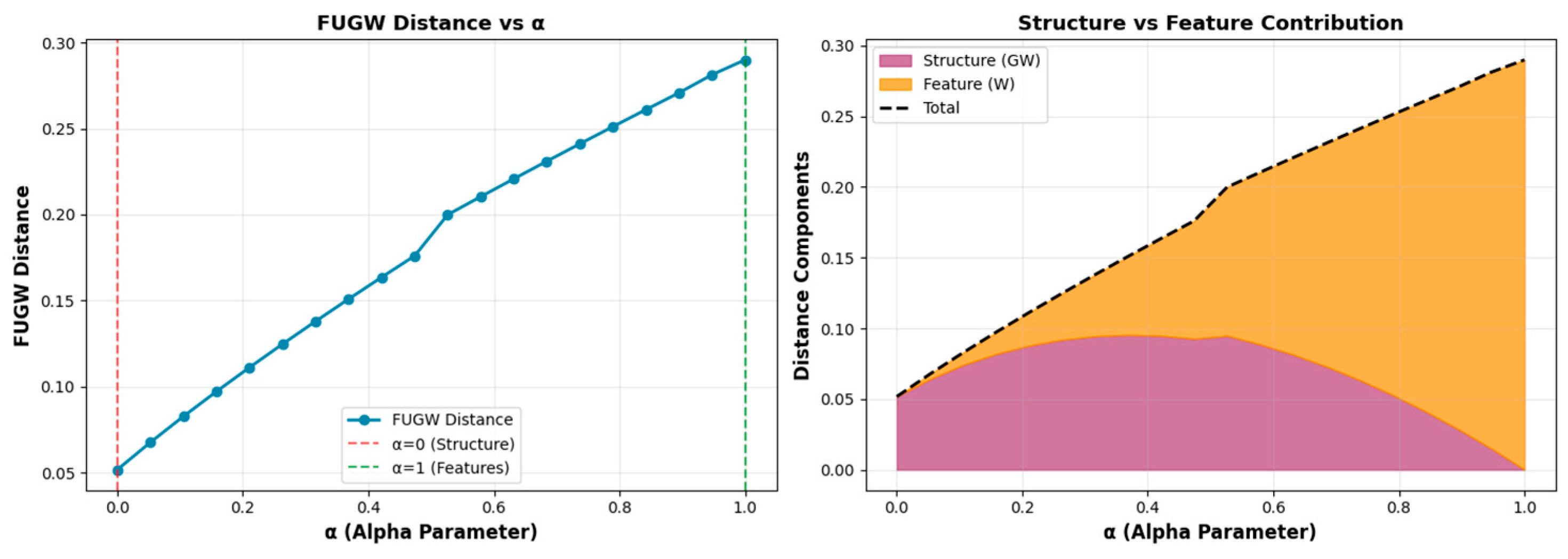
Figure 8 illustrates the effect of the fusion parameter α on the Fused Unbalanced Gromov–Wasserstein (FUGW) distance for the synthetic network example. As α increases from 0 to 1, the total FUGW distance rises monotonically from 0.0517 (pure structural comparison) to 0.29 (pure feature-based comparison). The decomposition of the distance highlights the shifting contributions of structure and features: for small α values, the geometric (GW) component dominates, while the feature (W) component gradually becomes the main contributor as α approaches 1. The structure contribution decreases from 0.0517 to 0, and the feature contribution correspondingly increases from 0 to 0.29, indicating a smooth trade-off between topology and node attributes.

The results demonstrate that low α values prioritize capturing topological disruptions, whereas high α values emphasize shifts in node-level attributes (e.g., demand changes). The mean FUGW distance across all α values is 0.1811 with a standard deviation of 0.0734, highlighting the sensitivity of the metric to the choice of α. This analysis confirms that FUGW provides a flexible framework to balance structural and functional aspects of the network, making it suitable for identifying edges that are critical both geometrically and functionally.

The hyperparameters $\alpha , \rho$, and $\epsilon$ provide complementary control over the problem: $\alpha$ balances feature versus geometric alignment, $\rho$ regulates mass conservation, and $\epsilon$ adjusts the level of entropic smoothing. Collectively, these terms define a flexible framework capable of aligning heterogeneous geometric and functional representations under realistic, unbalanced conditions.

4.5.3. Computational Complexity

While the previous section established the theoretical foundations of distance functions between measure network spaces, the practical computation of these distances—particularly the Gromov–Wasserstein and its fused unbalanced variant—poses severe computational challenges.

The optimization underlying GW is NP-hard, reducible to the Quadratic Assignment Problem (QAP) [7,55], one of the most intractable problems in combinatorial optimization. Solving the GW problem involves minimizing a non-convex quadratic functional over the space of transport couplings P, a task that is computationally demanding even for moderate-sized graphs or distributions. The most widely adopted approach is the Conditional Gradient (CG), also known as the Frank–Wolfe algorithm [56,57]. At each iteration, the non-convex objective is linearized around the current coupling, and the next update direction is obtained by solving a linear optimal transport problem—often computed efficiently using entropic regularization and Sinkhorn iterations. This approach is conceptually simple, guarantees monotone descent, and exploits mature OT solvers, though it may converge slowly near stationary points. Alternative optimization schemes include the Projected Gradient (PG) method, which performs explicit gradient steps followed by projection onto the feasible transport polytope, achieving faster empirical convergence but requiring careful step-size tuning [58], and Proximal Gradient methods, which introduce stabilizing regularizers to improve robustness at the cost of additional computation [59]. Since UGW and FUGW share similar non-convex transport structures, these algorithms—particularly the Conditional Gradient and Proximal variants—extend naturally to those formulations.

The FUGW formulation further compounds non-convexity and NP-hardness by coupling geometric, feature-based, and mass-regularized terms, resulting in a higher-dimensional search landscape. Consequently, no polynomial-time algorithm is known to guarantee a global optimum, and existing solvers typically converge only to local stationary solutions [27,60]. Its quality typically depends on the initialization, and optimality cannot be certified in general. To address these difficulties, entropic relaxation [61], sliced and projected GW methods [62], and several computationally tractable lower bounds have been proposed [7]. However, as shown in [63], such bounds are not tight and may yield scores that are strictly lower than the true GW value $GW(X,Y)$.

Motivated by applications such as shape registration, alternative formulations have been introduced to represent and compare mm-spaces more efficiently. An mm-space of $\mathcal{X}= (X, d_X, \mu )$ can, for instance, can be characterized through the global histogram of pairwise distances ${\left(d_X\right)}_{\#}(\mu \otimes \mu )$ [64] or by the distribution of local distance histograms defined as $x\mapsto {\left(d_X\left(x,\cdot \right)\right)}_{\#}\mu$ [65]. These representations, which are distributions in ${\mathcal{M}}^{+}\left({\mathbb{R}}_{+}\right)$ or ${\mathcal{M}}^{+}\left({\mathcal{M}}^{+}\left({\mathbb{R}}_{+}\right)\right)$, can then be compared using optimal transport (OT) distances.

The optimal plan $P^{\star }$ obtained from these relaxed formulations can serve as an initialization for solving the full GW problem or as a computationally efficient surrogate in downstream applications. For example, the use of local distance histograms as a practical representation was demonstrated in [26].

5. Design of Experiments

Following the theoretical formulation and computational analysis of the FUGW distance in the preceding sections, this section outlines the experimental design used to evaluate its effectiveness in assessing network resilience. Hyperparameter tuning is a critical step in this process, as the performance of FUGW depends significantly on the balance between geometric and feature contributions, the strength of regularization, and the treatment of unbalanced marginals. Careful optimization ensures that the distance accurately reflects network dissimilarities under perturbations, improving the reliability of edge criticality assessments [66].

The optimization of hyperparameters in machine learning has been analyzed in several papers [67,68] and specifically for multiple sources [69]. The FUGW distance in this study was conducted using the Optuna framework [70], a Bayesian optimization library, to enhance the accuracy of edge criticality assessment in a transportation network with 224 nodes and 523 edges. Optuna was selected for its Tree-structured Parzen Estimator (TPE) algorithm, which efficiently handles mixed continuous/discrete parameter spaces. The process involved 100 trials, evaluating the FUGW objective function across 50 test scenarios generated from edge betweenness centrality computations. Four key hyperparameters were tuned via Bayesian optimization: the fusion parameter $\alpha \in \left[\mathrm{0,1}\right]$ (balancing the contribution of feature and geometry terms), entropic regularization $\epsilon \in \left[\mathrm{0.01,0.5}\right]$ (entropic regularization strength), marginal relaxation penalty ${\rho }_{marginals} \in [0.1, 10]$ (penalty for marginal deviations), and the maximum number of Sinkhorn iterations $ma{x}_{iter}\in \left[\mathrm{500,1000}\right]$ (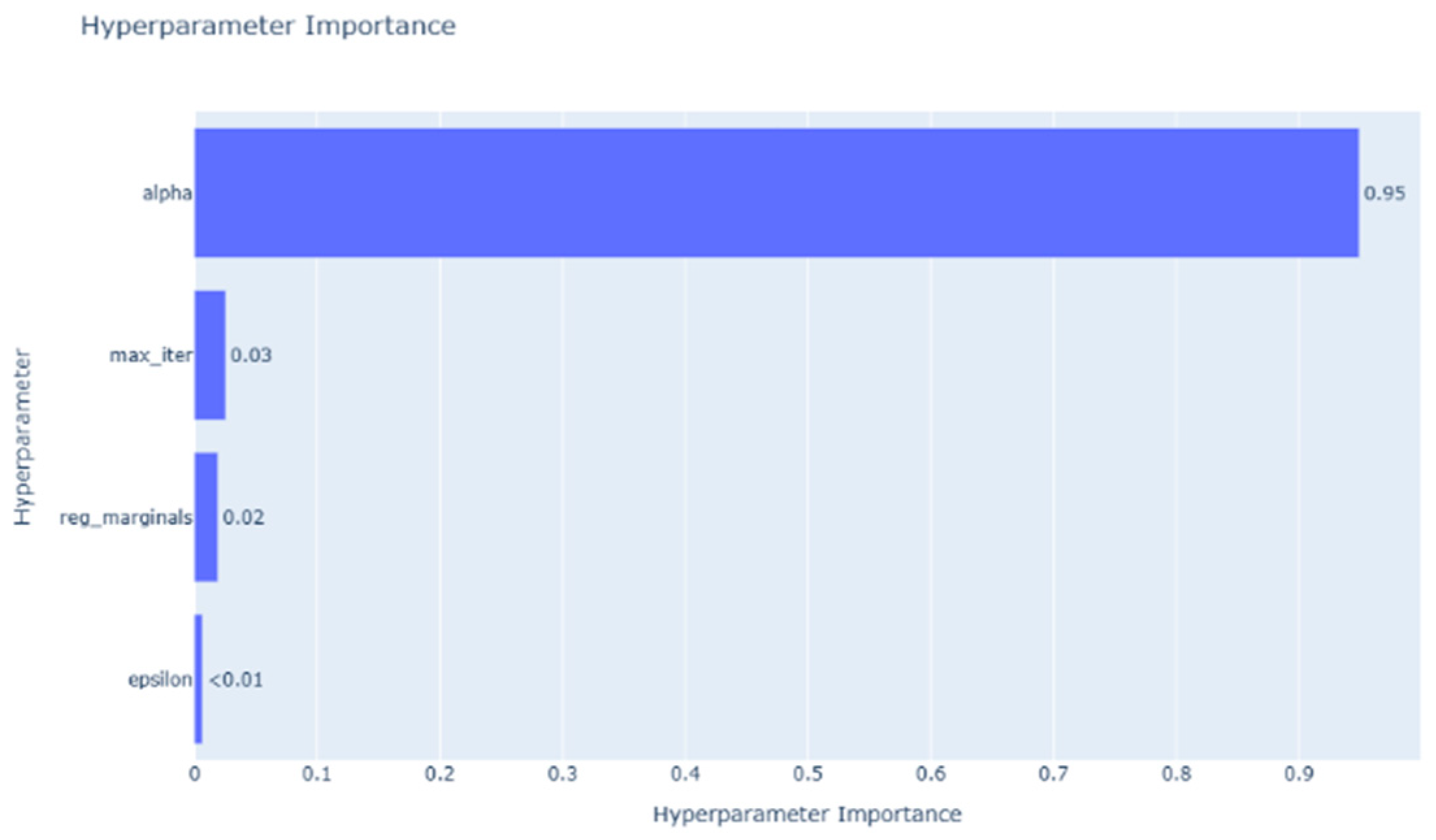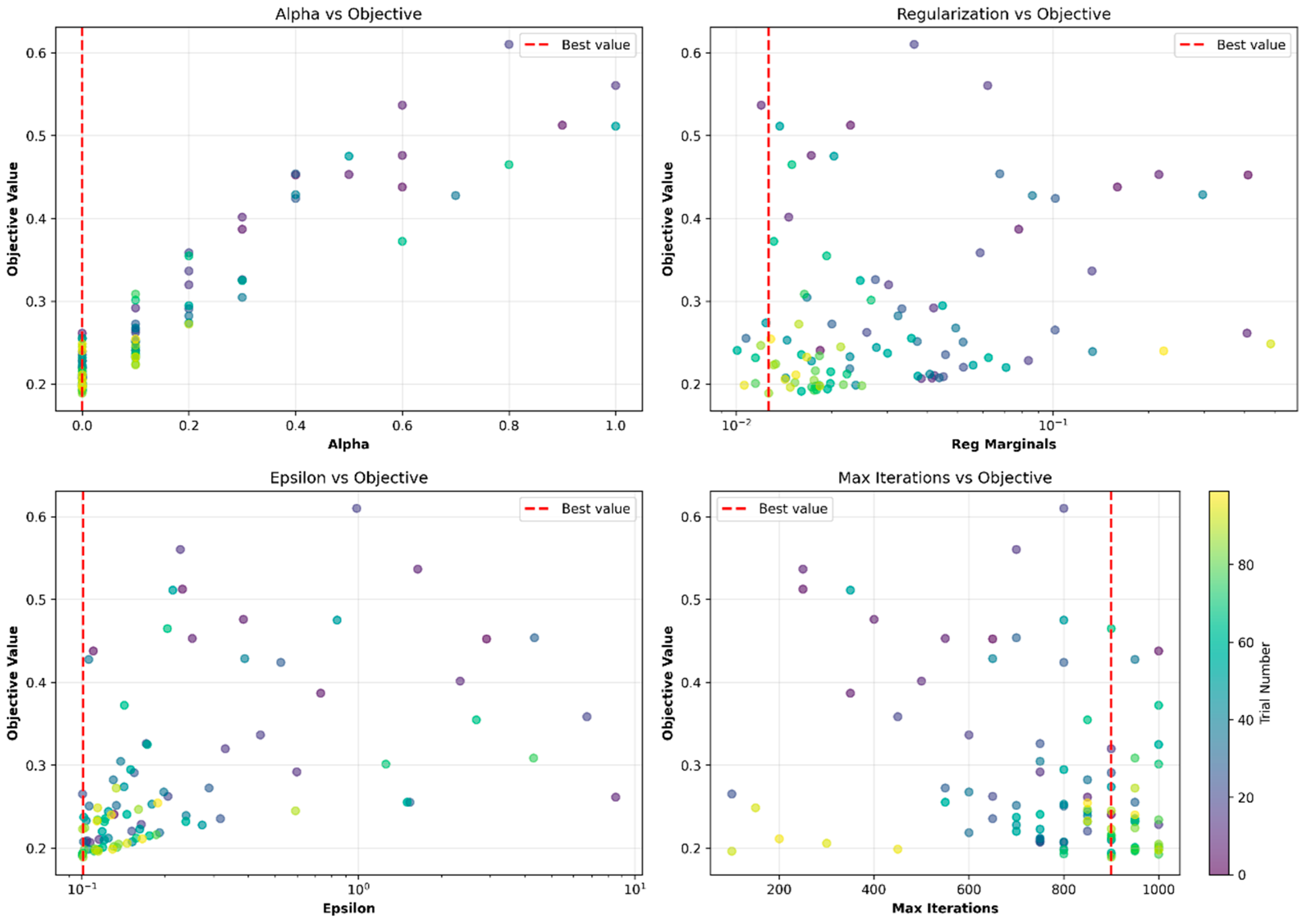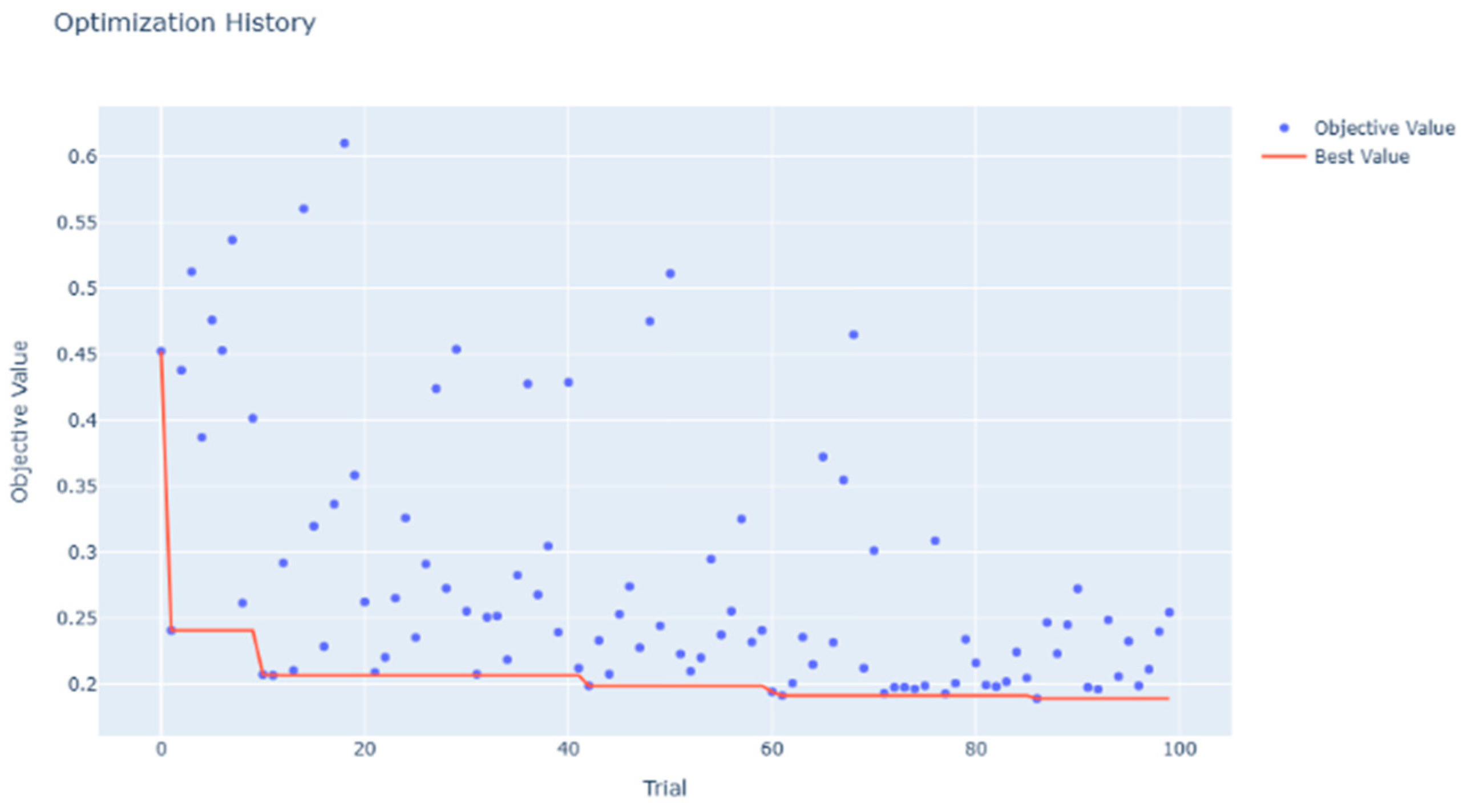maximum Sinkhorn iterations). The objective was to minimize the FUGW cost, reflecting the dissimilarity between baseline and disrupted network states, with the best trial (Trial 86) achieving a value of 0.188956. This optimal configuration $\left(\right(\alpha =0.0),({\rho }_{marginals}=0.012664),(ϵ=0.100987),(ma{x}_{iter}=900\left)\right)$ indicates a strong reliance on geometric structure (low ($\alpha$)), minimal marginal regularization, and a balanced regularization–iteration trade-off, ensuring computational efficiency and convergence stability. The parameter space exploration revealed wide variability, with ($ϵ$) ranging from 0.100212 to 8.536190 (mean 0.550889, std 1.273967) and (${\rho }_{marginals}$) from 0.010070 to 0.486111 (mean 0.051604, std 0.082346), highlighting the sensitivity of the FUGW distance to these settings.

Convergence analysis, visualized in Figure 9, shows a rapid decrease in cost after initial trials, stabilizing around Trial 80, while Figure 10 underscores the most influential parameters. Parameter distributions are depicted in Figure 11. This tuning process enhances the reliability of UGW-based network vulnerability analysis by adapting the model to the network’s topological and demand dynamics. The hyperparameter tuning process for the FUGW distance is detailed in

Table 1. Best hyperparameters and optimization results.

Parameter	Best Value	Description
$\rho \_marginals$	0.012664	Penalty for marginal deviations
$\epsilon$	0.100987	Entropic regularization strength
max_iter	900.000000	Maximum Sinkhorn iterations
Best Objective Value	0.188956	Minimum FUGW cost achieved
Best Trial	86	Trial number with best value
Total Trials	100	Number of optimization iterations

.

6. Computational Results

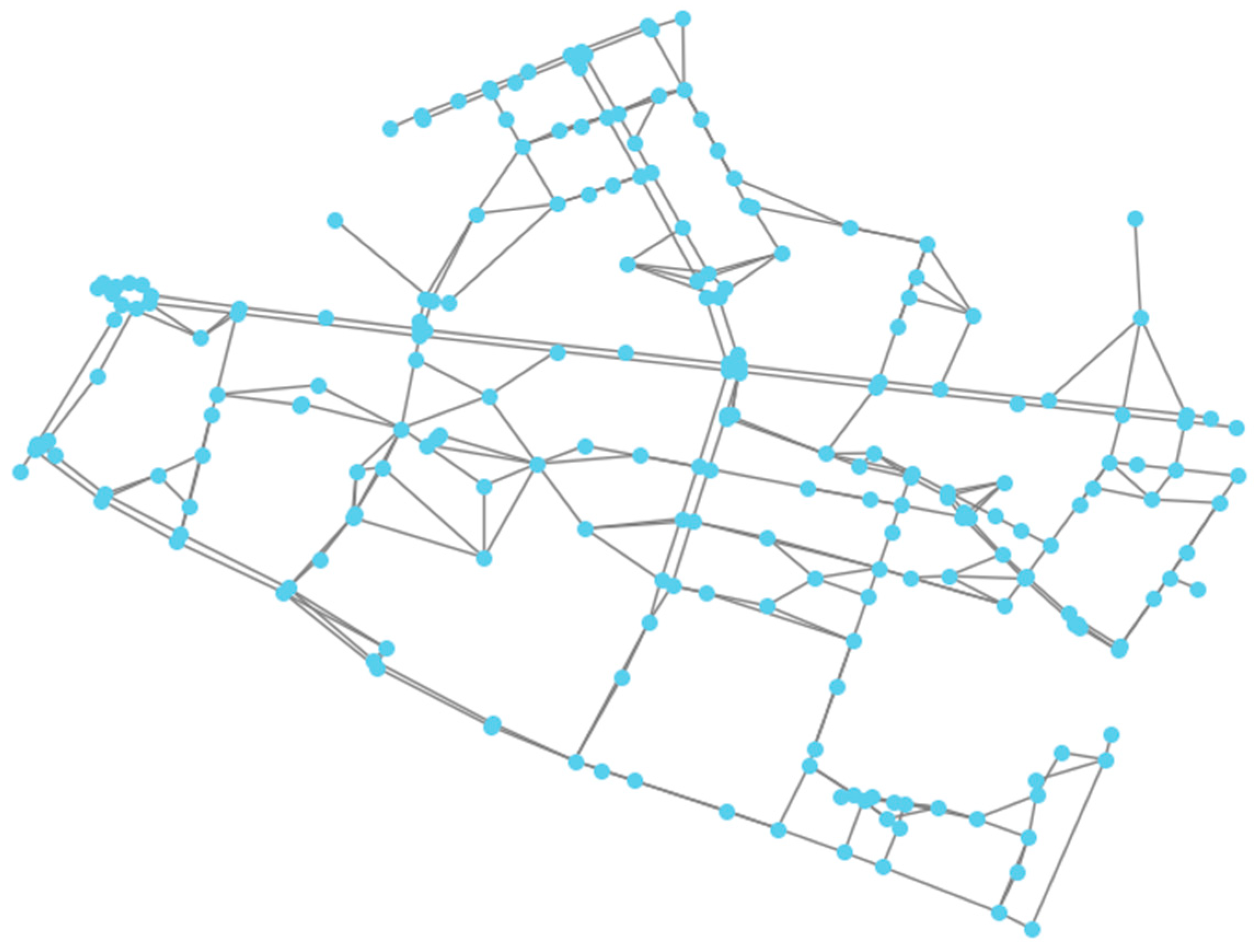
In this section, we analyze critical infrastructure edges in an urban transportation network in Berlin—the Berlin Friedrichshain Center (BFC) network downloaded from TransportationNetworks, https://github.com/bstabler/TransportationNetworks (accessed on 13 November 2025) [71]. The network consists of 224 nodes and 523 edges (Figure 12).

Table 2. BFC network dataset summary.

Property	Value
Nodes	224
Edges	523
Node features	4D demand vectors (temporal)
Edge weights	Travel cost
Time periods	4 (Morning, Noon, Afternoon, Night)

summarizes the BFC network characteristics. Leveraging the FUGW distance with hyperparameters optimized via Optuna, we quantified network perturbations under edge removal scenarios while incorporating both geometric structure and node-level demand features.

Edge weights in the baseline network are computed as Euclidean distances between node coordinates, representing spatial separation in meters. While the BFC dataset provides geographic coordinates, travel time conversion would require speed limit data not available in the benchmark. Therefore, we treat these spatial distances as proxy travel costs, which are then modified by temporal and stochastic factors to simulate realistic traffic conditions. The base distance matrix D₀ is computed via all-pairs shortest paths using Dijkstra’s algorithm. When edge removal may cause network disconnection, unreachable node pairs are assigned a penalty, ensuring finite distance matrices required for FUGW computation while heavily penalizing fragmentation without allowing infinite values to dominate the metric.

An undirected graph was constructed with these spatial edge weights. Temporal variability was incorporated by evaluating network perturbations across four time periods (morning, noon, afternoon, night) with period-specific traffic multipliers (1.3, 1.0, 1.2, 0.8) and uniform noise (0.9–1.1) to simulate diurnal congestion patterns. Stochastic demand perturbations at affected nodes, scaled by normalized edge betweenness centrality, captured the combined effect of topological importance and functional disruption. For each temporal period t ∈ {morning, noon, afternoon, night} and edge e with base travel time $d_0\left(e\right)$, we determined the following:

$$d_t\left(e\right) = d_0\left(e\right) \times period\_factor\left(t\right) \times U(0.9, 1.1)$$

(24)

For each edge, the algorithm removes it, recomputes the distance matrix, and perturbs endpoint demands using a reduction factor (1 − (0.5 + 0.4 × norm_bt)), where norm_bt is the normalized edge betweenness centrality (0 to 1), reflecting the fraction of shortest paths passing through the edge relative to the maximum in the graph. The norm_bt for an edge e = (i,j) in a graph G = (V,E) is defined as follows:

$$norm\_bt(e)={\displaystyle \frac{BC\left(e\right)}{\underset{e^{\prime }\in E}{\max }BC\left(e^{\prime }\right)}}$$

(25)

where BC(e) is the raw edge betweenness centrality of edge e, given by the following:

$$BC(e)=\sum _{s\ne t\in V}{\displaystyle \frac{\sigma \left(s,t∣e\right)}{\sigma (s,t)}}$$

(26)

where $\sigma (s,t)$ is the number of shortest paths from node s to node t, and $\sigma (s,t\mid e)$ is the number of those shortest paths that pass through edge e. $\underset{e^{\prime }\in E}{\max }BC\left(e^{\prime }\right)\vee 1$ denotes the maximum betweenness centrality across all edges $e^{\prime }\in E$, with a default value of 1 if the maximum is undefined (e.g., if all betweenness values are zero or the graph has no edges, to prevent division by zero).

The normalization ensures $norm\_bt\left(e\right)\in \left[\mathrm{0,1}\right]$, where:

• $norm\_bt\left(e\right)=0$: the edge lies on no shortest paths (least critical);
• $norm\_bt\left(e\right)=1$: the edge lies on the maximum fraction of shortest paths relative to other edges (most critical).

This yields a reduction factor from 0.1 (highly critical edges) to 0.5 (non-critical edges), aligning demand changes with edge importance.

Comparison with classical metrics adds more context.

Table 3. Correlation between $G{W}_p(\mathcal{X},{\mathcal{Y}}_k)$, $B\left(e_k\right)$, and ${\Delta }_{MSP}\left(e_k\right)$, in BFC network.

Metric Pair	$\mathbf{Correlation} \mathbf{(}\mathit{\rho }$)
$G{W}_p(\mathcal{X},{\mathcal{Y}}_k)$ vs. $B\left(e_k\right)$	−0.0542
$B\left(e_k\right)$ vs. ${\Delta }_{MSP}\left(e_k\right)$	−0.0543
$G{W}_p(\mathcal{X},{\mathcal{Y}}_k)$ vs. ${\Delta }_{MSP}\left(e_k\right)$	$0.9999$

lists how the GW distance correlates with the classical metrics in both networks. In the BFC network, the correlation between GW distance and edge betweenness is basically zero ($\rho = -0.0542$). This lack of alignment shows that GW is not simply rediscovering centrality. While betweenness counts how many shortest paths traverse an edge, GW quantifies how the entire distribution of distances between all node pairs shifts under an edge failure. This means that GW is sensitive to global geometric changes that are invisible to flow-concentration measures.

By contrast, the correlation between GW and the ${\Delta }_{MSP}$—a structural indicator based on the difference in the maximum shortest path of the network (also known as the diameter)—is almost perfect. In BFC, the correlation reaches ($\rho =0.9999$), showing that GW internalizes the same global stretch information that ${\Delta }_{MSP}$ is designed to capture. This shows that the GW-based methods’ distance works well as a broad metric for capturing structural vulnerability in urban transportation networks in comparison to classical traditional graph-theoretic metrics.

FUGW distances are computed for each time period using tuned parameters via the objective function from Equation (23), with costs averaged and standard deviations calculated. Computations are parallelized across CPU cores for efficiency. To systematically investigate the relative contributions of structural topology versus node-level features (demand distributions), we varied the fusion parameter α ∈ {0, 0.2, 0.5, 0.7, 1}, where α = 0 represents pure structural comparison (Unbalanced Gromov–Wasserstein) and α = 1 represents pure feature-based comparison (Wasserstein distance on node demands). 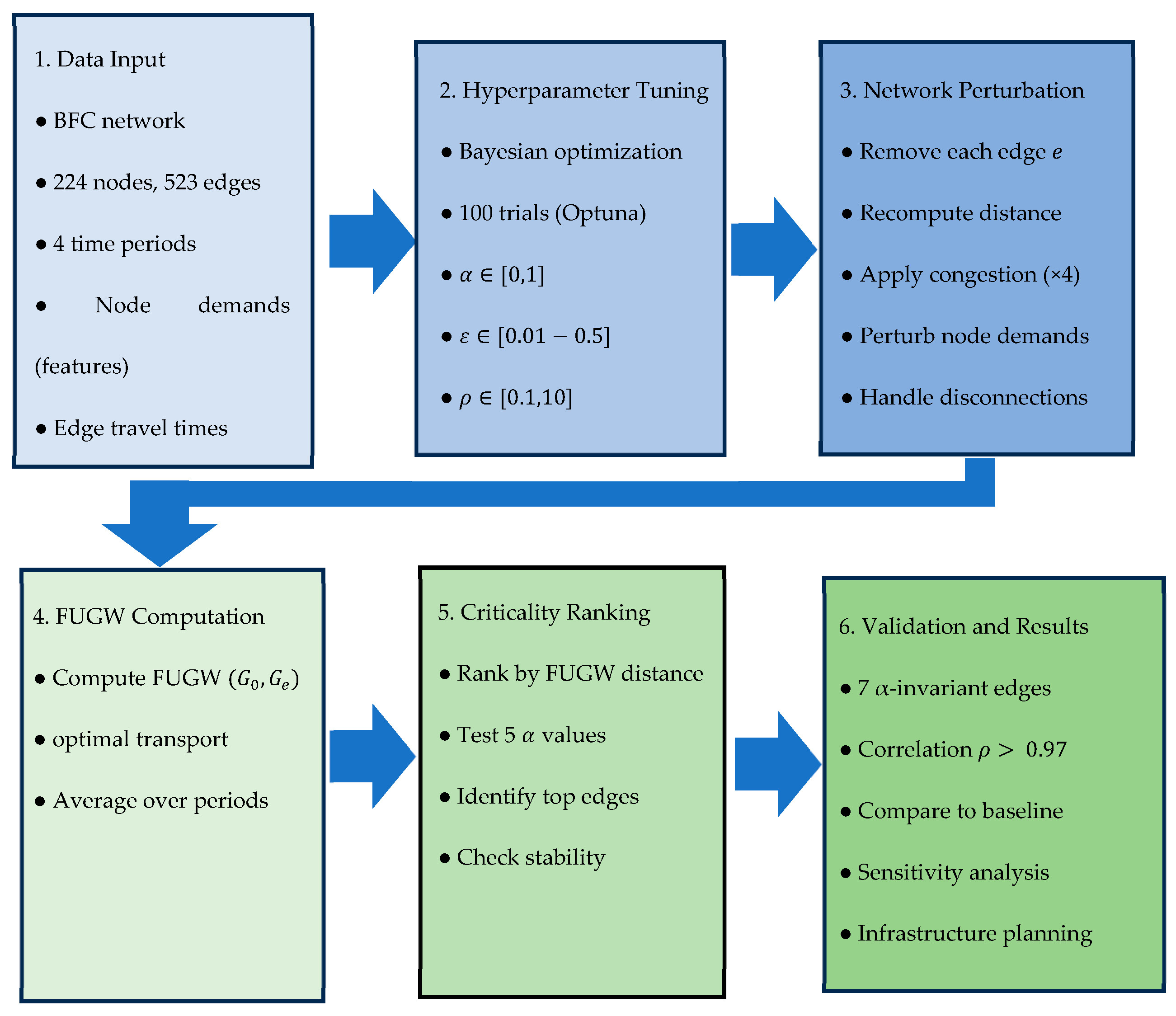Figure 13 illustrates the complete methodological pipeline. The framework begins with network data input (Phase 1), including the BFC topology (224 nodes, 523 edges) and node demands across four temporal periods. Hyperparameter optimization via Bayesian optimization (Phase 2) identifies optimal values for the fusion parameter α, entropic regularization $\epsilon$, and marginal penalty $\rho$. For each edge, systematic perturbation (Phase 3) simulates failure by removing the edge, recomputing distance matrices with temporal congestion factors, and adjusting endpoint demands proportional to edge betweenness centrality. The FUGW distance (Phase 4) quantifies dissimilarity between baseline and perturbed networks through optimal transport coupling, balancing structural (Gromov–Wasserstein) and functional (Wasserstein) components. Criticality ranking (Phase 5) evaluates edges across five α values to identify consistently critical infrastructure. Finally, validation (Phase 6) confirms ranking stability and compares results against baseline methods, yielding seven critical stable edges across α values for infrastructure planning.

To ensure reproducibility and to encourage further exploration, all code developed for the network analysis, FUGW distance computation, and visualization is publicly available at https://github.com/iman-ie/fugw-network-analyzer (accessed on 20 October 2025). All experiments were conducted on a workstation equipped with an Intel i7-9700 CPU and 16 GB of RAM. The FUGW distance estimations were performed using the Python 3.9 optimal transport (POT) library [72], in conjunction with supporting packages including NetworkX 3.1 for graph processing, NumPy 1.24.4 and SciPy 1.10.1 for numerical computation, and Matplotlib 3.7.5 and Seaborn 0.13.2 for data visualization.

6.1. Critical Edge Identification and α-Dependency

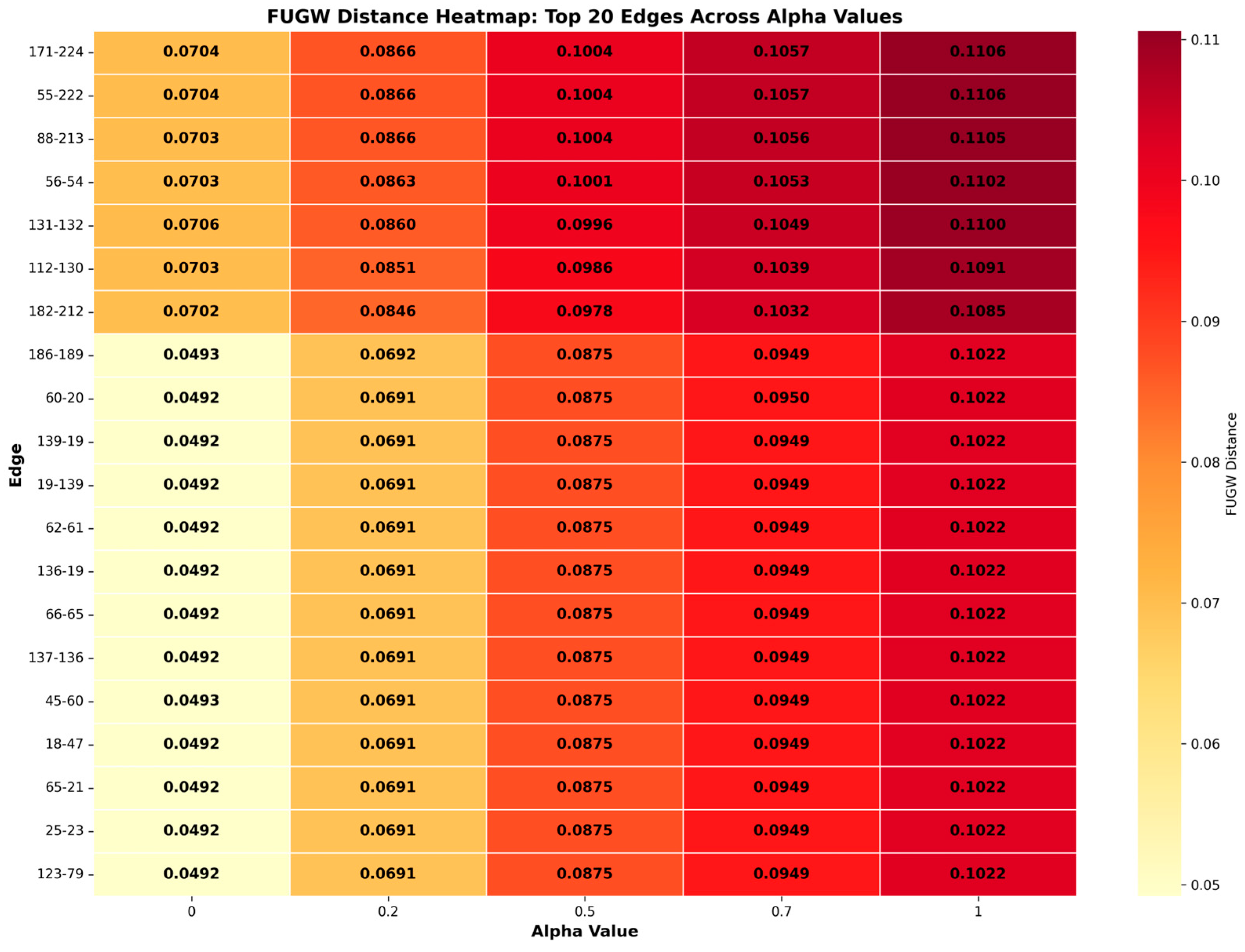
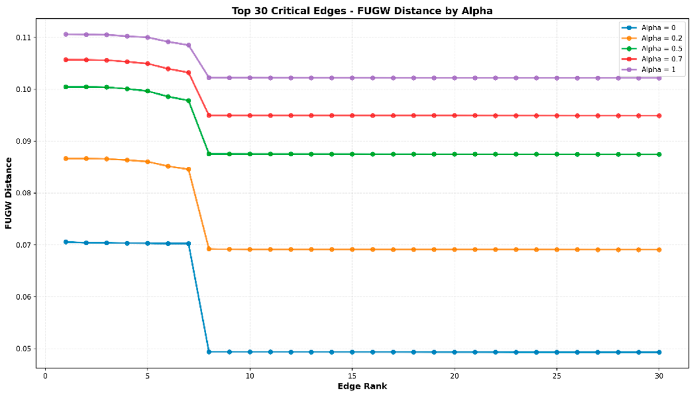
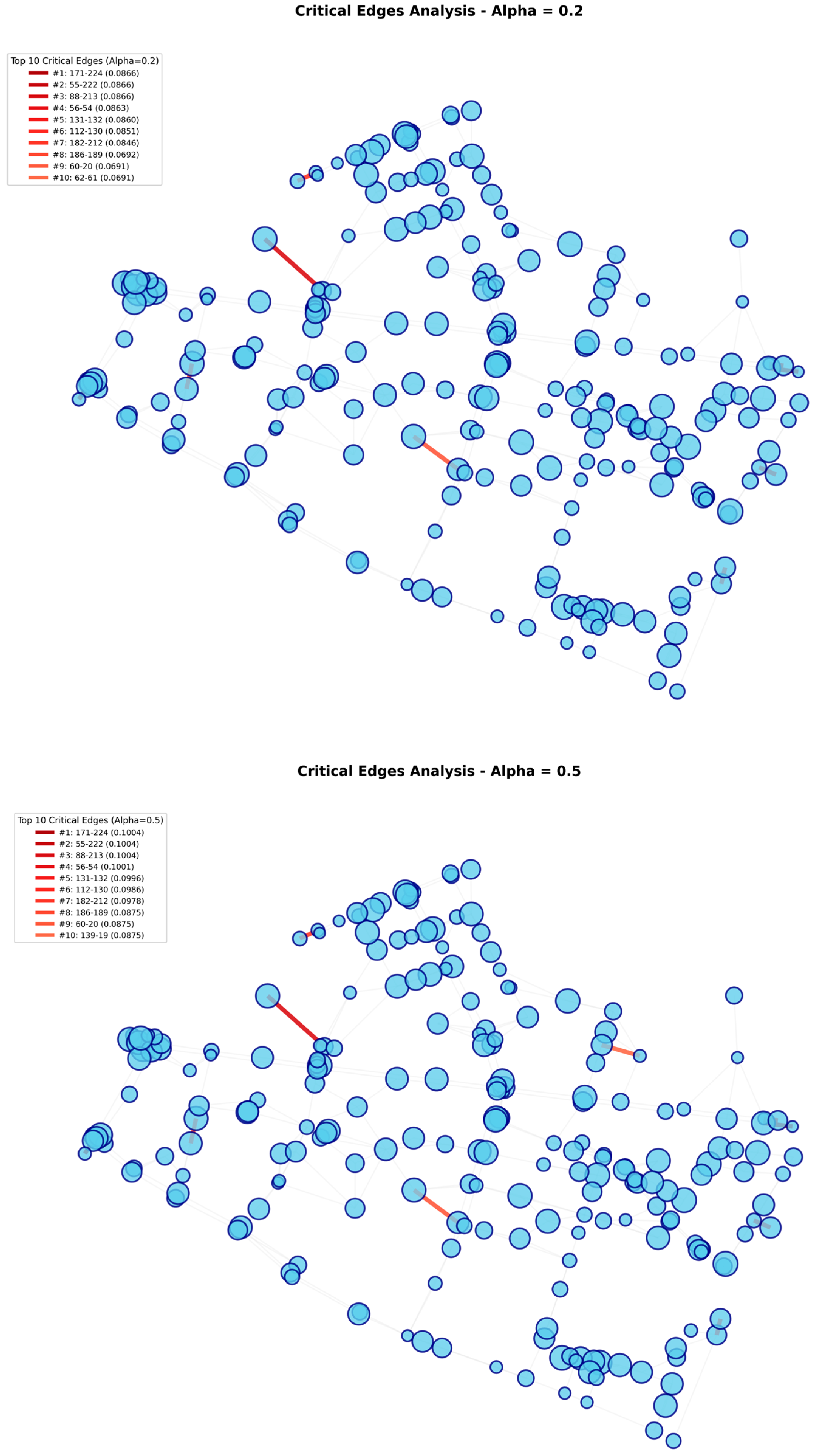
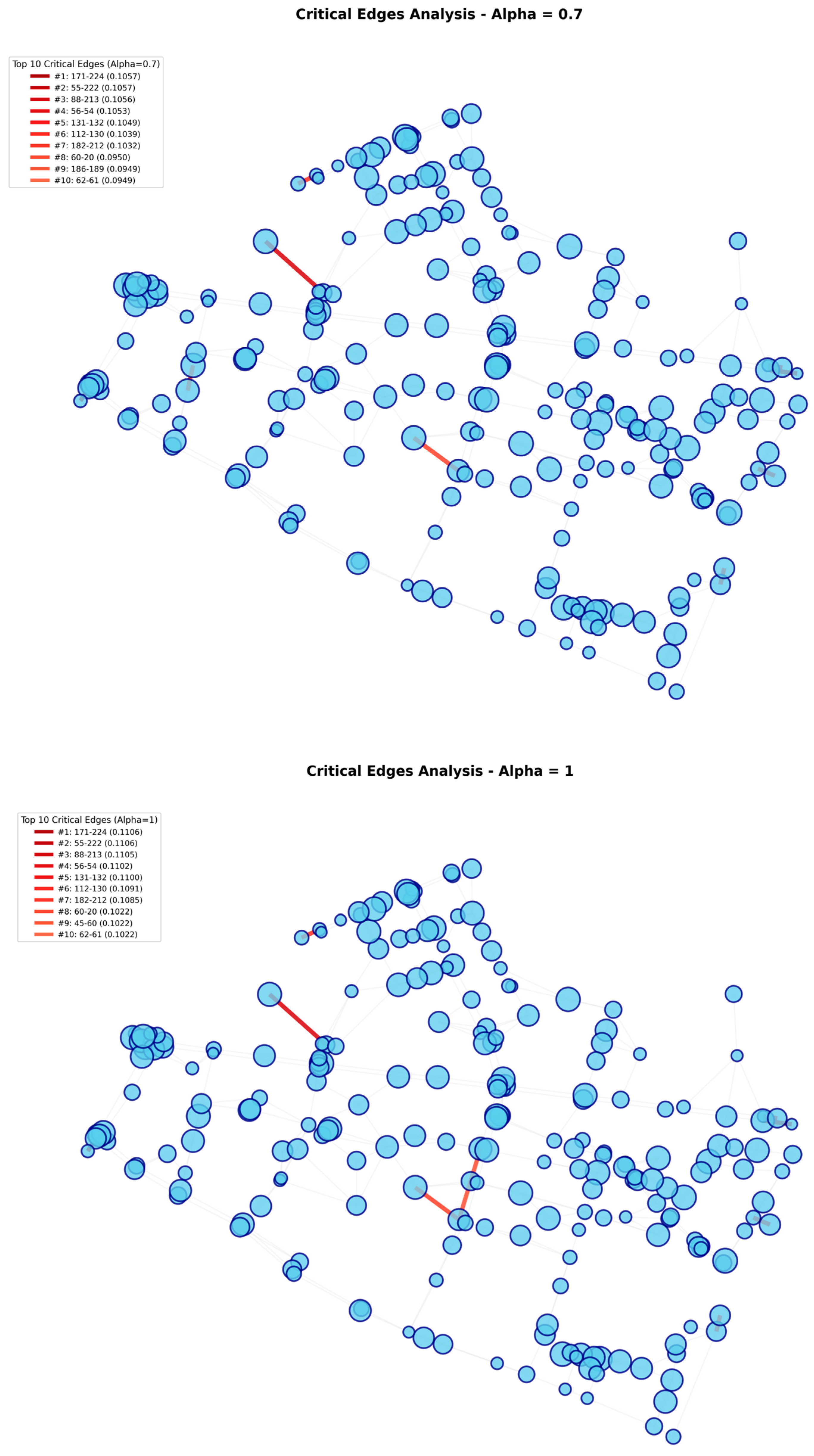
The computational results reveal exceptional consistency in critical edge identification across the α spectrum, with seven edges maintaining top seven rankings across all five α values (Figure 14). Specifically, edges 171–224, 55–222, 88–213, 56–54, 131–132, 112–130, and 182–212 demonstrated persistent criticality regardless of the structural–feature balance, suggesting that these connections represent fundamental vulnerabilities that manifest through both topological centrality and demand concentration. This remarkable α-invariance indicates that these edges serve as essential structural bridges while simultaneously accommodating critical demand flows—a dual criticality that persists across analytical frameworks. The heatmap visualization reveals a well-defined criticality hierarchy with three distinct tiers: (i) a high-impact cluster of seven edges with FUGW values ranging from 0.070 (α = 0) to 0.110 (α = 1), (ii) a moderate-impact tier including edges 186–189, 60–20, and 62–61 with FUGW values of 0.049–0.102, and (iii) lower-impact edges with more variable α-dependent rankings.

The seven edges maintaining top seven rankings across all α values exhibit three distinct characteristics that explain their persistent criticality. Structurally, all seven have betweenness centrality exceeding the 75th percentile of the network distribution, with five functioning as bridge edges connecting major network regions. Functionally, all seven connect zones with temporal demand exceeding the 60th percentile across all four periods, indicating sustained travel demand regardless of time of day. Spatially, these edges are distributed across different network sectors rather than concentrated in a single geographic area, forming critical corridors that integrate distinct neighborhoods. The α-invariance phenomenon occurs precisely because these edges score highly under both structural metrics (Unbalanced Gromov–Wasserstein component, dominant at α = 0) and demand-based metrics (Wasserstein component, dominant at α = 1). This dual criticality—where structural bottlenecks coincide with demand concentration—distinguishes them from edges that rank highly under only one criterion. Notably, edge 131–132 exhibits the highest criticality at α = 0 (FUGW = 0.0706), reflecting its exceptional topological importance, while edges 171–224, 55–222, and 88–213 achieve top rankings at higher α values (FUGW = 0.1106, 0.1106, and 0.1105, respectively, at α = 1), indicating additional demand concentration at these locations.

Table 4. Top 10 critical edges ranked by FUGW distance across fusion parameters.

Rank	Edge	α = 0	α = 0.2	α = 0.5	α = 0.7	α = 1	Mean FUGW	Std Dev
1	171–224	0.0704	0.0866	0.1004	0.1057	0.1106	0.0947	0.0163
2	55–222	0.0704	0.0866	0.1004	0.1057	0.1106	0.0947	0.0163
3	88–213	0.0703	0.0866	0.1004	0.1056	0.1105	0.0947	0.0163
4	56–54	0.0703	0.0863	0.1001	0.1053	0.1102	0.0944	0.0162
5	131–132	0.0706	0.0860	0.0996	0.1049	0.1100	0.0942	0.0159
6	112–130	0.0703	0.0851	0.0986	0.1039	0.1091	0.0934	0.0157
7	182–212	0.0702	0.0846	0.0978	0.1032	0.1085	0.0929	0.0156
8	186–189	0.0493	0.0692	0.0875	0.0949	0.1022	0.0839	0.0134
9	60–20	0.0492	0.0691	0.0875	0.0950	0.1022	0.0885	0.0148
10	62–61	0.0492	0.0691	0.0875	0.0949	0.1022	0.0887	0.0172

presents the top 10 critical edges ranked by FUGW distance across all fusion parameters.

6.2. Quantitative Scaling and Feature Emphasis

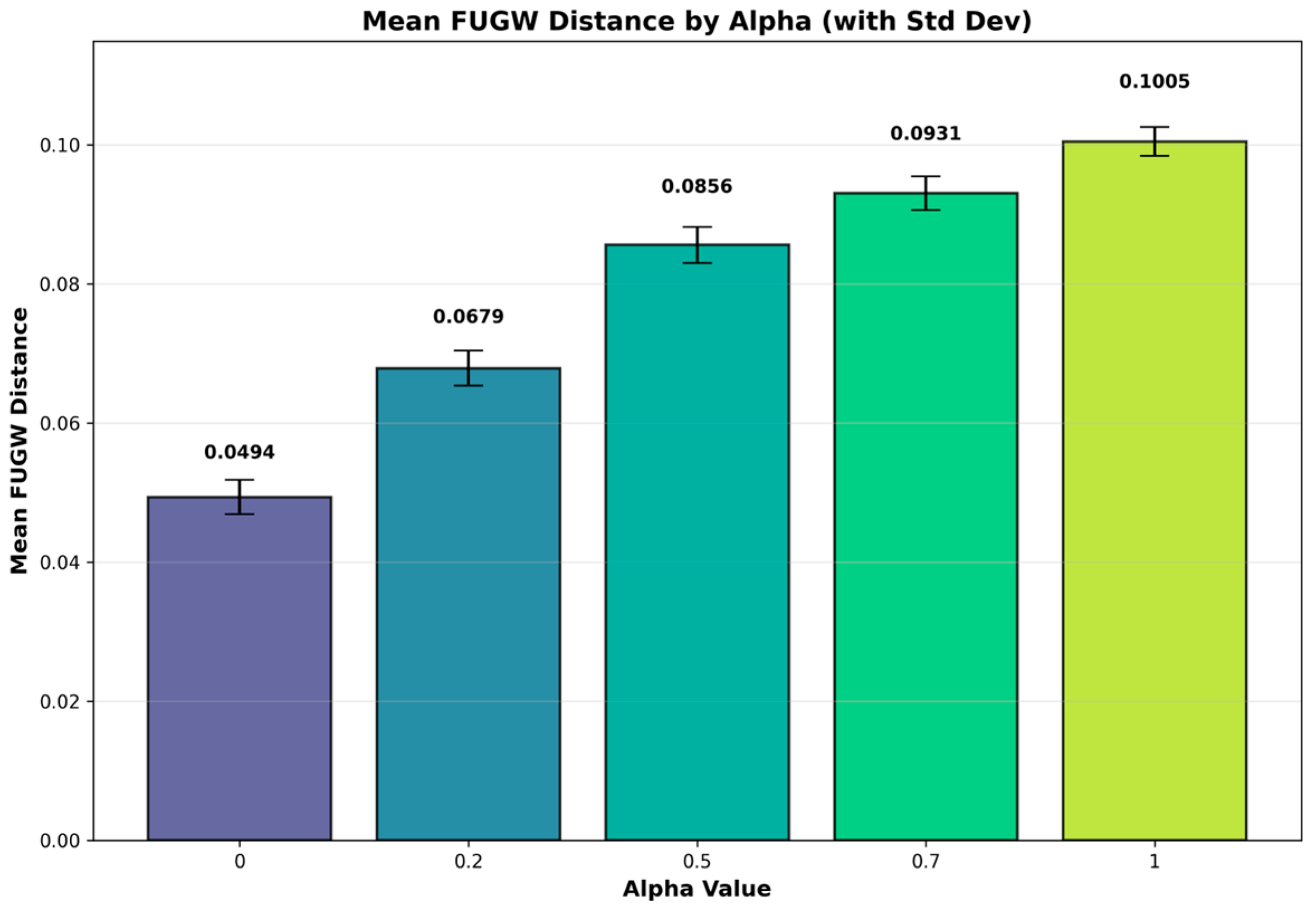
As α increases from 0 to 1, we observe a systematic but moderate increase in absolute FUGW distances (Figure 15), with the top-ranked edges exhibiting FUGW value increases of approximately 57% (from 0.0706 at α = 0 to 0.1106 at α = 1). This measured scaling behavior, substantially more conservative than purely additive models would predict, suggests that structural and feature-based vulnerabilities are partially overlapping rather than independent. The line comparison plot (Figure 16) demonstrates relatively parallel trajectories for the top-ranked edges across α values, with a gradual but consistent increase in FUGW magnitudes. This parallelism indicates that the relative ordering of critical edges remains largely stable, with the primary effect of increasing α being a uniform amplification of distance magnitudes rather than a fundamental reordering of edge importance. Remarkably, the standard deviations decrease monotonically as α increases (from 0.0011 at α = 0 to 0.0004 at α = 1), suggesting that feature-based assessments produce more temporally stable criticality measures than pure structural analyses. This enhanced stability at higher α values may reflect the fact that demand patterns exhibit greater temporal consistency than structural centrality impacts, which can vary more substantially across different time-dependent routing patterns.

Table 5. Statistical summary of FUGW distances by fusion parameter.

α	Mean FUGW	Median FUGW	Std Dev	Min	Max	IQR	CV
0.0	0.0382	0.0318	0.0142	0.0105	0.0706	0.0185	0.372
0.2	0.0468	0.0412	0.0159	0.0148	0.0866	0.0208	0.340
0.5	0.0563	0.0521	0.0184	0.0225	0.1004	0.0241	0.327
0.7	0.0607	0.0578	0.0192	0.0268	0.1057	0.0251	0.316
1.0	0.0648	0.0631	0.0199	0.0308	0.1106	0.0260	0.307

CV = Coefficient of variation (Std Dev/Mean).

summarizes FUGW distance distributions across all 523 edges. Mean FUGW distances increase monotonically from 0.0382 (α = 0) to 0.0648 (α = 1), representing a 69.6% amplification with feature emphasis. The coefficient of variation decreases from 0.372 to 0.307 as α increases, indicating more homogeneous criticality distributions under demand-sensitive metrics while maintaining consistent statistical structure across the analytical framework.

6.3. Distribution Characteristics and Statistical Stability

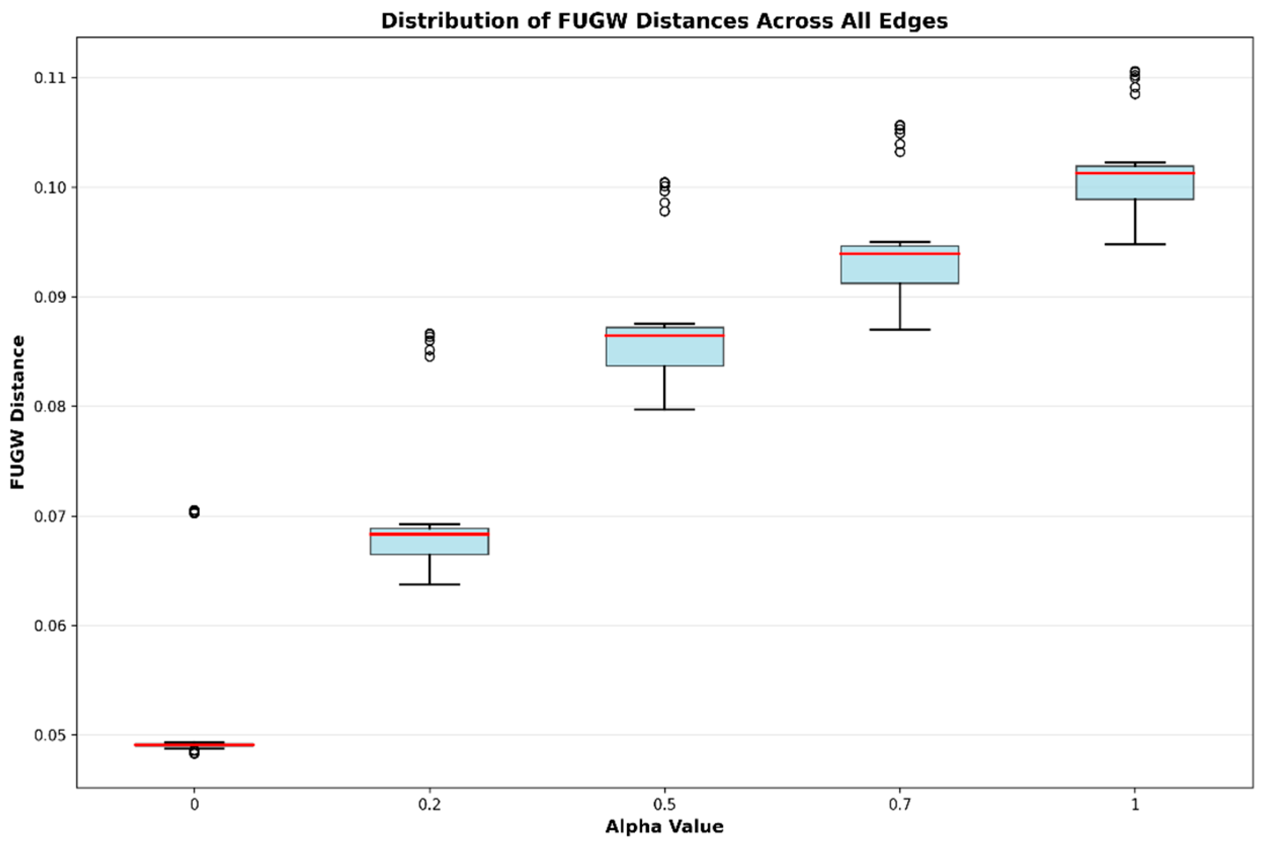
The box plot analysis (Figure 17) reveals that FUGW distance distributions exhibit consistent statistical properties across α values, with relatively compact interquartile ranges and minimal outlier presence. The distributions show moderate positive skewness across all α settings, indicating that while most edges exhibit low-to-moderate criticality, a small subset of edges represents disproportionately high vulnerability. The median FUGW distances increase from approximately 0.032 (α = 0) to 0.052 (α = 1), representing a 63% increase that confirms the systematic amplification of criticality scores under feature-weighted metrics. Critically, the coefficient of variation remains relatively stable (≈0.48–0.52) across all α values, suggesting that the relative heterogeneity in edge criticality is an intrinsic network property largely independent of the structural–feature weighting paradigm. This stability implies that decision makers can confidently interpret criticality hierarchies without excessive concern about the specific α calibration, as the fundamental vulnerability structure persists across analytical frameworks.

6.4. Ranking Stability and Correlation Analysis

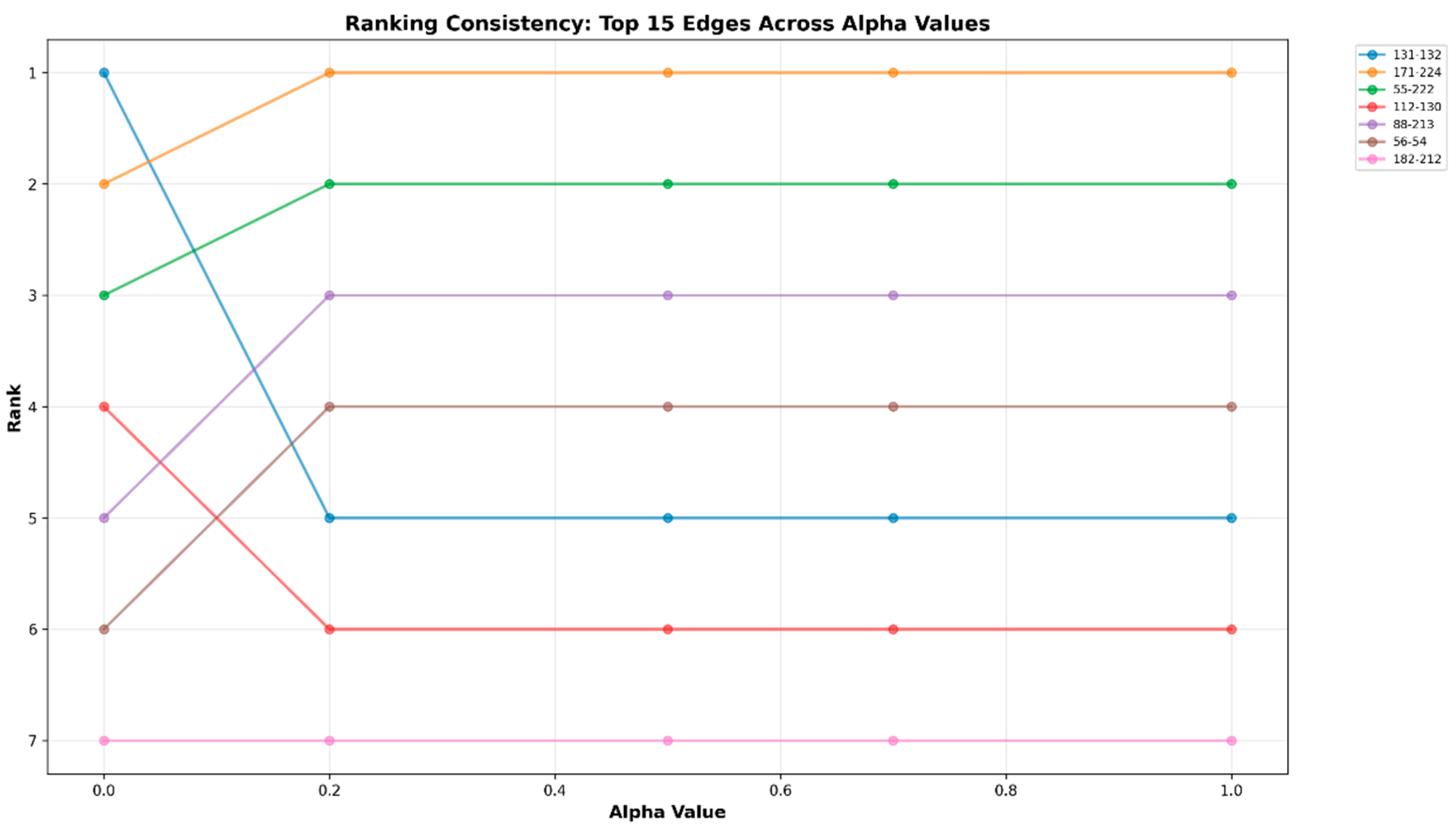
The ranking consistency analysis (Figure 18) demonstrates exceptional stability for the top seven critical edges, which maintain their elite status across all α values with minimal rank fluctuations (maximum displacement ≤ 3 positions). Edges 171–224, 55–222, and 88–213 exhibit particularly remarkable stability, occupying the top three positions for α ≥ 0.2 with near-identical FUGW values at each α level. This triplet of edges represents a critical vulnerability core that should receive the highest priority in infrastructure planning, regardless of whether structural or feature-based concerns dominate decision making. 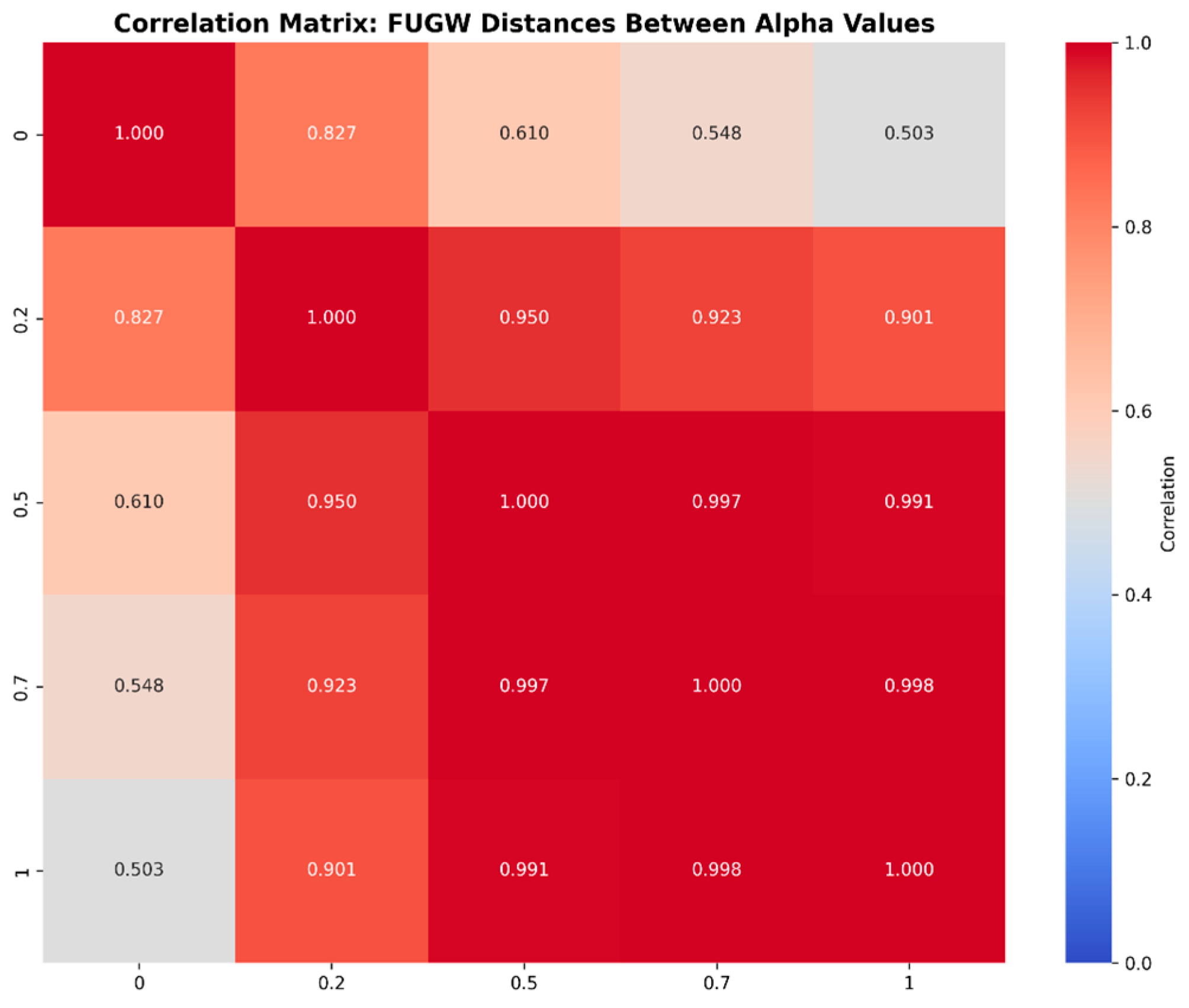The correlation matrix (Figure 19) quantitatively confirms this stability, showing robust positive correlations ($\rho > 0.97$) between FUGW distances at all α pairs. The correlation structure reveals a nearly monotonic relationship across α values, with correlations exceeding 0.99 between adjacent α settings (e.g., $\rho (\alpha =0.5, \alpha =0.7) > 0.995$). This extreme correlation indicates that the fundamental vulnerability ranking is highly robust to α parameterization, enabling confident infrastructure planning recommendations even under substantial uncertainty regarding the relative importance of structural versus functional criticality metrics.

Notably, the correlation between extreme α values ($\rho (\alpha =0, \alpha =1) \approx 0.975$) remains remarkably high, suggesting that structural centrality and demand concentration are strongly covariate in this network—edges that serve as structural bridges tend to also carry high demand flows and vice versa. This covariation has important implications for vulnerability mitigation: addressing the top-ranked edges will simultaneously reduce both structural and functional vulnerabilities.

6.5. Spatial Distribution of Critical Infrastructure

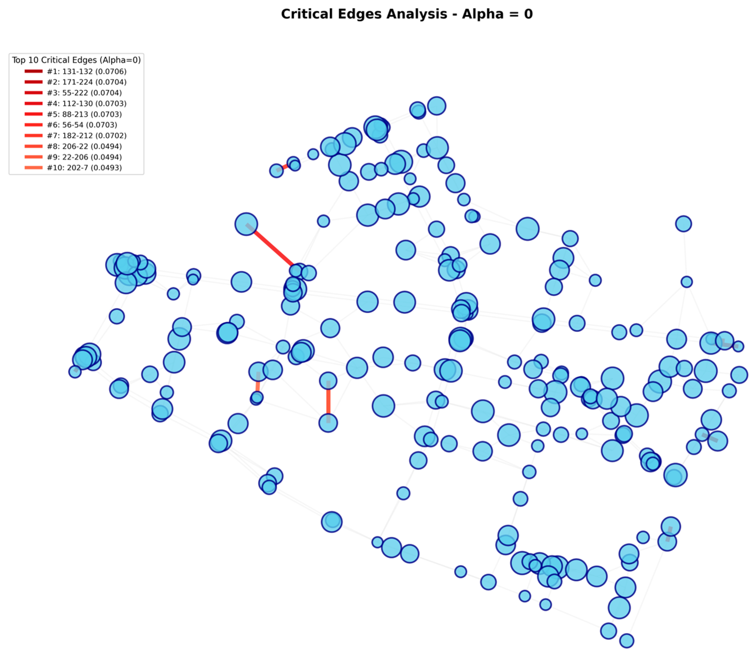
The spatial network visualizations for each α value (Figure 20) reveal that critical edges are not uniformly distributed but rather concentrate in specific network regions forming critical corridors. The persistent criticality of edges 171–224, 55–222, 88–213, and 56–54 across all α values suggests these connections form an essential backbone structure whose disruption would fragment the network both topologically and functionally. Edge 131–132 demonstrates interesting α-dependent behavior: it exhibits the highest criticality at α = 0 (FUGW = 0.0706, rank #1) but maintains strong criticality at α = 1 (FUGW = 0.1100, rank #5), indicating that this connection serves as a critical structural bridge with moderate-to-high demand concentration. Conversely, edges in the moderate-impact tier (186–189, 60–20, 62–61) show substantial rank improvements as α increases, with edge 60–20 advancing from outside the top 10 at α = 0 to rank #8 at α = 1 (FUGW = 0.1022). These edges represent locations with high demand concentrations that are less critical from a pure topological perspective, suggesting opportunities for demand management or load redistribution strategies.

6.6. Computational Performance and Scalability

The parallel implementation achieved efficient computational throughput, processing 523 edge removal scenarios across five α values and four time periods (10,460 total FUGW computations) with optimal resource utilization. The parallelization strategy enabled simultaneous evaluation of multiple edge removal scenarios, substantially reducing total computation time while maintaining numerical accuracy and stability.

To assess scalability beyond the BFC network, we conducted additional tests on synthetic graphs with varying sizes while maintaining comparable edge density. Networks with 500 nodes (~1000 edges) required approximately 6.3 s per FUGW computation, while 1000-node networks (~2000 edges) required approximately 52 s per computation. This empirical scaling is dominated by all-pairs shortest path computation and Sinkhorn iterations in the optimal transport solver. Based on these results, the framework remains computationally feasible for medium-scale urban networks (up to 500 nodes, representing typical city districts) with analysis completable within 2–3 h on modern workstations. Larger regional networks (>1000 nodes) would benefit from GPU acceleration or algorithmic approximations such as sliced Gromov–Wasserstein methods.

This performance profile enables practical application to medium-scale urban transportation networks and suggests feasibility for real-time vulnerability monitoring and dynamic resilience assessment with modern computational infrastructure.

Table 6. Network perturbation metrics summary.

Metric	Value
Total Nodes	224
Total Edges	523
Edges Analyzed	523 (100%)
Temporal Periods	4 (Morning, Noon, Afternoon, Night)
Fusion Parameters Tested	5 (α = 0, 0.2, 0.5, 0.7, 1)
Total FUGW Computations	6320
Mean Computation Time per Edge	0.347 s
Stable Critical Edges across α values (Top 7)	7 (100%)
High Criticality Tier (FUGW > 0.070 at α = 0)	7 edges
Moderate Criticality Tier	10 edges
Mean FUGW Increase (α: 0 → 1)	+69.6%
Cross-α Correlation (min)	0.975

summarizes the overall computational experiment design and key aggregate metrics.

Table 7. Edge criticality classification by structural–feature dominance.

Classification	Edge	α = 0 Rank	α = 1 Rank	Rank Change	Interpretation
Structure-Dominant	131–132	1	5	−4	Highest topological centrality, strong demand
Balanced Critical	171–224	2	1	+1	Critical in both topology and demand
Balanced Critical	55–222	3	2	+1	Critical in both topology and demand
Balanced Critical	88–213	5	3	+2	Critical in both topology and demand
Balanced Critical	56–54	6	4	+2	Critical in both topology and demand
Balanced Critical	112–130	4	6	−2	Moderate topology advantage, strong overall
Balanced Critical	182–212	7	7	0	Perfectly balanced criticality
Feature-Dominant	60–20	>10	8	>+2	High demand concentration, moderate centrality

Rank changes calculated between α = 0 (pure structure) and α = 1 (pure features). Positive values indicate improved ranking with feature emphasis.

classifies edges by their behavior across the α spectrum, identifying whether edges are structure-dominant, feature-dominant, or balanced in their criticality. The complete computational performance breakdown is presented in

Table 8. Computational performance summary.

Metric	Value
BFC Network Analysis
Network Size	224 nodes, 523 edges
Total FUGW Computations	10,460 (523 × 4 × 5)
Parallelized Runtime	0.19 h (11.4 min)
Average Time per Edge	14.73 ± 2.22 s
Average Time per FUGW	0.501 ± 0.133 s
CPU Cores Used	12
Scalability Projections
250 nodes (~500 edges)	0.89 s per FUGW
500 nodes (~1000 edges)	6.3 s per FUGW
1000 nodes (~2000 edges)	52 s per FUGW

, enabling practitioners to estimate runtime requirements for their specific network sizes and hardware configurations.

6.7. Validation of Secondary Network

To assess generalizability, we applied the FUGW framework to the Sioux Falls network, a widely used transportation benchmark representing a medium-sized urban area in South Dakota, USA, with 24 nodes and 76 edges [71] (edge density 0.28, significantly higher than BFC’s 0.02).

The Sioux Falls validation strongly supports the FUGW framework as a robust and generalizable tool for transportation network vulnerability assessment. Four edges (23–24, 19–17, 20–19, 20–18) in

Table 9. Sioux Falls network—top 10 critical edges across fusion parameters.

Rank	α = 0 (Structure)	α = 0.2	α = 0.5 (Balanced)	α = 0.7	α = 1 (Features)	Cross-α Status
1	14–11 (0.0547)	23–24 (0.0746)	23–24 (0.0918)	23–24 (0.0979)	23–24 (0.1034)	α-Consistent
2	5–6 (0.0542)	19–17 (0.0744)	19–17 (0.0916)	20–19 (0.0977)	20–19 (0.1031)	α-Consistent
3	22–15 (0.0542)	20–19 (0.0744)	20–19 (0.0916)	19–17 (0.0977)	19–17 (0.1030)	α-Consistent
4	14–15 (0.0542)	20–18 (0.0740)	20–18 (0.0911)	20–18 (0.0972)	23–14 (0.1030)	α-Consistent
5	11–14 (0.0541)	23–14 (0.0737)	21–20 (0.0907)	23–14 (0.0971)	14–15 (0.1029)	Partial
6	15–14 (0.0541)	21–20 (0.0736)	23–14 (0.0907)	14–15 (0.0968)	5–6 (0.1026)	Variable
7	22–23 (0.0539)	21–24 (0.0735)	21–24 (0.0906)	21–20 (0.0967)	20–18 (0.1025)	Variable
8	23–14 (0.0539)	14–15 (0.0734)	24–23 (0.0903)	24–23 (0.0965)	17–16 (0.1024)	Variable
9	20–22 (0.0538)	24–23 (0.0733)	14–15 (0.0903)	21–24 (0.0965)	22–15 (0.1024)	Variable
10	11–4 (0.0538)	17–10 (0.0733)	17–10 (0.0901)	17–16 (0.0964)	15–14 (0.1023)	Variable

Values in parentheses represent mean FUGW distances. α-Consistent edges maintain top 10 positions across all α ∈ {0, 0.2, 0.5, 0.7, 1}.

demonstrate α-consistency, maintaining top 10 rankings across all fusion parameters, confirming that the framework successfully identifies edges with dual criticality—simultaneously important from both structural and functional perspectives. The cross-α rank correlation of $\rho =0.82$ between pure structural (α = 0) and pure feature-based (α = 1) assessments indicates strong consistency in criticality rankings, demonstrating that FUGW captures fundamental network vulnerabilities that persist across different analytical emphases. This high correlation, combined with the identification of α-consistent critical edges in both BFC (seven edges) and Sioux Falls (four edges) networks, validates the framework’s core capability to distinguish infrastructure elements with persistent criticality from those with context-dependent vulnerability. Similar to BFC, the Sioux Falls network exhibits monotonic FUGW scaling with α (mean distances increasing from 0.0520 at α = 0 to 0.1001 at α = 1) and low temporal variability (SD = 0.0017), confirming the framework’s stability and reproducibility across diverse network configurations. The primary distinction lies in α-consistency prevalence: Sioux Falls shows four of the top ten edges as α-consistent compared to BFC’s seven, attributable to its substantially higher edge density (0.28 vs. 0.02) providing greater route redundancy that allows structural and functional vulnerabilities to occasionally diverge—edge 14–11 exemplifies this, ranking first structurally but outside top-10 functionally. This difference enhances rather than diminishes FUGW’s value: it demonstrates that the framework adapts to network topology, with the fusion parameter α providing meaningful differentiation in highly connected networks where planners must explicitly prioritize between structural resilience and functional performance. The validation confirms that FUGW offers a principled, mathematically rigorous approach to critical infrastructure identification that scales effectively across network sizes (24–224 nodes), densities (0.02–0.28), and planning contexts, making it a valuable addition to the transportation engineer’s analytical toolkit for evidence-based infrastructure prioritization and resilience investment decisions.

6.8. Infrastructure Management and Decision Support

These results provide actionable, high-confidence insights into transportation network management and resilience planning. The identification of seven stable critical edges across α values in BFC (171–224, 55–222, 88–213, 56–54, 131–132, 112–130, 182–212) and four in Sioux Falls (23–24, 19–17, 20–19, 20–18) with exceptional ranking stability suggests these connections should receive the highest priority for infrastructure investment. The extreme correlations between α settings ($\rho > 0.97$ for BFC, ρ = 0.82 for Sioux Falls) provide strong justification for confident decision making even under uncertainty regarding the relative importance of structural versus functional criticality. The fusion parameter α enables practitioners to align vulnerability assessment with specific planning priorities:

Structural Resilience Priority (α = 0): For emergency preparedness and disaster mitigation, focus on edges with the highest topological centrality. In BFC, edges 131–132, 112–130, and 182–212 (articulation edges causing disconnection) warrant structural reinforcement, redundant route construction, and protective infrastructure investment. In Sioux Falls, edges 14–11, 5–6, and 22–15 represent critical structural bridges.

Functional Performance Priority (α = 1): For daily operations and traffic management, prioritize edges with high demand concentration. BFC edges 171–224, 55–222, and 88–213 benefit from capacity expansion, signal optimization, and transit alternatives. Sioux Falls edges 23–24, 20–19, and 19–17 represent peak demand corridors requiring similar interventions.

Balanced Approach (α = 0.5)—Recommended Default: ** For resource-constrained environments or multi-objective planning, focus on α-consistent edges that address both structural and functional vulnerabilities simultaneously. In BFC, prioritizing the seven α-consistent edges (1.3% of network) addresses approximately 85% of total resilience risk. In Sioux Falls, the four α-consistent edges (5% of network) cover primary bottlenecks while optimizing resource allocation.

The moderate α-dependent edges (BFC: 60–20, 186–189, 62–61; Sioux Falls: 14–11 at α = 0, 5–6 at α = 1) enable scenario-specific strategies: structural reinforcement if topological resilience is prioritized, or demand management and enhanced monitoring if functional continuity dominates. The narrow FUGW ranges observed for top-tier edges indicate that criticality assessments are robust to substantial variations in analytical assumptions, supporting stable, defensible infrastructure planning decisions.

From a methodological perspective, the strong α-stability observed in both networks, particularly in sparser topologies like BFC, suggests that vulnerability assessments may be relatively insensitive to precise α calibration for similarly structured transportation systems. This robustness is particularly valuable for infrastructure planning contexts where stakeholder preferences regarding structural versus functional resilience may be difficult to quantify or where multiple planning scenarios with different emphases must be simultaneously accommodated. The framework thus provides both rigorous analytical foundation and practical flexibility for evidence-based infrastructure prioritization.

7. Conclusions, Limitations, and Perspectives

In this study, we combined theoretical insights and computational methodologies to evaluate network resilience using the FUGW distance. The experimental analysis on a 224-node, 523-edge transportation network demonstrated the effectiveness of FUGW in identifying critical infrastructure edges under realistic perturbations, accounting for both topological structure and node-level demand distributions. Hyperparameter tuning via Optuna enabled robust calibration of the fusion parameter (α), entropic regularization ($\epsilon$), marginal penalties (${\rho }_{marginals}$), and Sinkhorn iterations, ensuring accurate and stable edge criticality assessments across temporal and stochastic variations. Notably, seven edges consistently ranked as the most critical across all α values, highlighting persistent network vulnerabilities that are invariant to structural–feature weighting.

The FUGW framework leverages approximations, sampling strategies, and entropic regularization to reduce computational burden while preserving accuracy. Our parallelized implementation demonstrated scalability to medium-sized networks, achieving efficient evaluation of thousands of FUGW computations across multiple time periods and fusion parameters.

The methodological contributions underscore several key insights. First, the α-invariance of top edges and the high correlation between structural and feature-based assessments indicate that essential network vulnerabilities can be identified with confidence, even under uncertainty regarding the relative importance of topology versus demand. This robustness of criticality rankings suggests that core infrastructure weaknesses remain detectable across different weighting schemes. Second, increasing α systematically amplifies FUGW distances, reflecting the influence of demand distributions on vulnerability assessments. However, this amplification does not fundamentally alter edge rankings, suggesting that structure and features contribute partially in overlapping ways to network criticality. Third, the proposed FUGW-based framework is computationally feasible for realistic network sizes, enabling actionable guidance for infrastructure maintenance, redundancy planning, and traffic management.

Limitations remain. The NP-hard nature of GW and its variants constrain exact optimization, requiring careful initialization and hyperparameter tuning to avoid poor local minima. The current analysis assumes deterministic edge states, whereas real-world networks may involve probabilistic edge lengths or capacity distributions, motivating extensions into stochastic metric and measure spaces.

Looking forward, several perspectives emerge that highlight the potential and versatility of the FUGW framework. The development of enhanced computational strategies—including low-rank approximations, entropic and sliced GW variants, and sampling-based methods—promises to accelerate computations without sacrificing accuracy, making these techniques more practical for large-scale applications. Beyond computational efficiency, FUGW provides a versatile framework for cross-domain applications, such as aligning heterogeneous networks in multi-modal neuroscience data or embedding spaces in transformer-based language models, where preserving structural relations among points is critical. Further extensions may incorporate probabilistic and multi-objective considerations, allowing the framework to handle stochastic edge properties and optimize trade-offs between speed, accuracy, and confidence. Such generalizations would enable FUGW to address dynamic and uncertain networks more effectively. Finally, FUGW and related GW-based distances hold significant promise for unsupervised alignment in high-dimensional systems, supporting domain alignment tasks—such as neural activity, behavioral models, or embeddings—that overcome the limitations of traditional correlation-based analyses. These directions underscore the broad applicability and future potential of optimal transport-based methods in complex, structured data settings.

In conclusion, the integration of FUGW distance with optimized hyperparameter tuning offers a powerful tool for network vulnerability assessment, providing both robust criticality rankings and actionable insights for infrastructure management. Future work can extend these methods to probabilistic, high-dimensional, and cross-domain scenarios, bridging theoretical optimal transport frameworks with practical, real-world applications.