A Computational Framework for FFR Estimation in Right Coronary Arteries: From CFD Simulation to Clinical Validation

Abstract

Coronary artery disease (CAD) remains the leading cause of cardiovascular mortality worldwide. Accurate and non-invasive quantification of coronary hemodynamics, namely in the right coronary artery (RCA), is essential for clinical decision-making but remains challenging due to the complex interaction among vessel geometry, pulsatile flow, and blood rheology. This study presents and validates a transparent computational framework for non-invasive fractional flow reserve (FFR) estimation using patient-specific RCA geometries reconstructed from coronary computed tomography angiography (CCTA) using SimVascular 27-03-2023. The proposed workflow integrates realistic boundary conditions through a Womersley velocity profile and a three-element Windkessel outlet model, coupled with a viscoelastic blood rheology formulation (sPTT) implemented via user-defined functions (UDFs). This work integrates all clinically relevant conditions of invasive FFR assessment into a single patient-specific computational framework, while delivering results within a time frame compatible with clinical practice, representing a meaningful methodological advance. The methodology was applied to seven patient-specific cases, and the resulting non-invasive FFR values were compared with both invasive wire-based measurements and commercial HeartFlow^® outputs (Mountain View, CA, USA). Under hyperemic conditions, the computed FFR values showed strong agreement with invasive references, with a mean relative error of 8.4% ± 6.3%, showing diagnostic consistency similar to that of HeartFlow^® (8.3% ± 8.1%) for the selected dataset. These findings demonstrate the ability of the proposed CFD-based pipeline to accurately replicate physiological coronary behavior under hyperemia. This novel workflow provides a fully on-site, open-source, reproducible, and cost-effective framework. Ultimately, this study advances the clinical applicability of non-invasive CFD tools for the functional assessment of CAD, particularly in the RCA.

1. Introduction

Cardiovascular diseases (CVDs) are the leading cause of death globally, accounting for an estimated 19.8 million deaths in 2022, or approximately 32% of all global deaths,85% of which were due to heart attack and stroke [1]. It is estimated that 43% of all CVD deaths are related to coronary artery disease (CAD), which primarily results from the progressive accumulation of atherosclerotic plaques that narrow the coronary lumen and impair myocardial perfusion [2,3]. The physiological impact of such stenoses is clinically assessed through the fractional flow reserve (FFR), defined as the ratio between distal and aortic pressures during maximal vasodilation (hyperemia). This non-dimensional parameter ranges from 0 (a completely obstructed vessel) to 1 (a healthy vessel). FFR values ≤ 0.80 indicate flow-limiting lesions requiring revascularization or other intervention, whereas higher values suggest that optimal management can be achieved with medical therapy [4,5]. Despite its diagnostic accuracy, the invasive nature of FFR measurement—requiring catheter insertion and pharmacologically induced hyperemia—introduces procedural risk, patient discomfort, and increased healthcare costs [6].

Computational simulation has become a key tool for the analysis of nonlinear systems in real-world applications, particularly when analytical solutions are impractical due to complex interactions between geometry, material behavior, and boundary conditions. In biomedical contexts, such nonlinearities are intrinsic to physiological systems, where controlled numerical modeling enables systematic exploration of system responses and parameter sensitivities under realistic conditions. By allowing virtual experimentation that would be difficult or impossible to perform in vivo, simulation-based approaches play an essential role in bridging theoretical models with practical applications and supporting informed decision-making in applied sciences [7].

In recent years, non-invasive alternatives for FFR estimation have emerged to address these drawbacks, leveraging coronary computed tomography angiography (CCTA) and computational fluid dynamics (CFD) to simulate coronary hemodynamics virtually [2,8]. By combining anatomical imaging with physiologically realistic computational modeling, these methods enable the calculation of pressure and flow distributions along patient-specific arteries, replicating invasive FFR measurements without catheterization. Commercial platforms such as HeartFlow^® have demonstrated the clinical feasibility of this concept, but they remain proprietary “black boxes” and are often cost-prohibitive for routine use [9]. Consequently, open-source, reproducible, and adaptable CFD workflows are increasingly pursued in academic settings to enhance accessibility, methodological transparency, and scientific validation.

Early frameworks demonstrated the feasibility of coupling three-dimensional coronary CFD with lumped-parameter models (LPM) of the circulation, but they were often computationally demanding and parameter-rich, complicating patient-specific application and increasing uncertainty. Kwon et al. (2014) implemented a patient-specific CFD–LPM approach in which only the coronary tree was meshed while a simplified coronary LPM provided boundary conditions [10]. This reduced runtime relative to models also meshes the aorta, while producing FFR values consistent with invasive readings in their test case. However, the method still relied on several unmeasured parameters—such as the distribution of branch resistances and compliances based on total coronary flow—and did not report hyperemic microvascular calibration beyond scaling resting flow, which may bias distal pressure predictions. The authors explicitly acknowledged the difficulty of identifying LPM parameters in a truly patient-specific manner [10]. Other groups have investigated how modeling choices themselves alter non-invasive FFR. Using a reconstructed coronary tree with artificially induced lesions, Chahour et al. (2020) compared generalized (Carreau-type) non-Newtonian flow against Navier–Stokes with different outlet conditions, showing that Windkessel boundary conditions materially affect pressure fields [11]. Their study, however, was primarily methodological rather than a patient-specific validation against invasive FFR.

Alongside boundary conditions, blood rheology is critical for accurate pressure-drop prediction. More recently, Pinto et al. (2020) implemented viscoelastic rheology in ANSYS Fluent^® 2025R1 via user-defined functions (UDFs) and showed, in RCA geometries, that non-linear viscoelastic models such as multi-mode simplified Phan-Thien/Tanner (sPTT) reduce peak wall shear stress by around 50% compared with shear-thinning Carreau and flatten core velocities [12]. These effects are most pronounced in regions where velocity gradients are high, such as post-stenosis and bifurcations, emphasizing that viscoelasticity is not a negligible refinement in coronary flows.

Despite these advances, persistent limitations remain in previous studies targeting non-invasive FFR estimations, particularly in the RCA. First, boundary conditions are often simplified or only partially physiological. Several studies assume steady or generic inflow profiles or omit explicit modeling of downstream behavior, which can distort pressure waves and lead to inaccurate FFR estimation [13,14]. Secondly, constitutive modeling is frequently limited to Newtonian or purely shear-thinning laws, even though viscoelastic effects are known to influence RCA hemodynamics precisely where FFR-relevant gradients occur [12,15,16]. Finally, validation against invasive FFR has typically been restricted to small demonstrations with partially idealized assumptions, performed in left coronaries, or presented with proprietary pipelines that lack transparency on the exact modeling choices, hindering independent verification and reproducibility [17,18].

In this study, we address these gaps and present a transparent, reproducible, and patient-specific pipeline for non-invasive FFR estimation that integrates: (i) CCTA-based 3D reconstruction and hyperemia transformation (the condition that patients are under during the invasive procedure), followed by robust meshing; (ii) physiologically consistent pulsatile inflow via a Womersley velocity profile; (iii) three-element Windkessel boundary conditions to represent distal behavior; and (iv) a viscoelastic sPTT model for blood rheology, previously shown to better capture coronary hemodynamics.

From a practical standpoint, the proposed framework follows a clinically realistic imaging-to-physiology workflow. Patient-specific RCA geometries are reconstructed from routinely acquired CCTA data and simulated using a realistic CFD setup. The model provides a non-invasive estimate of FFR under conditions mimicking the invasive procedure, intended for real-world use as an on-site, transparent, reproducible, and editable alternative for functional assessment of CAD, particularly in the RCA.

2. Materials and Methods

The current section details the entire pipeline used to calculate the non-invasive FFR, including the dataset of all studied patients, the 3D reconstruction of patient-specific RCAs, the transformation of the RCAs in a hyperemic condition, the definition of the blood rheology model, and the respective boundary conditions. All the implemented numerical settings for the simulations conducted in ANSYS Fluent^® are also described.

2.1. Patients Dataset

This study included adult patients (age ≥ 18 years) with suspected CAD, referred for clinically indicated CCTA at the Cardiology Department of Unidade Local de Saúde Gaia e Espinho (ULSGE), Portugal. The selection criteria targeted patients with confirmed obstructive CAD in the RCA, defined in a vessel with a diameter of ≥2 mm, based on visual estimation of CCTA.

Invasive FFR was measured during coronary angiography using a pressure-sensor guidewire according to standard interventional cardiology practice. Following engagement of the target coronary artery with a guiding catheter, intracoronary nitrates were administered to minimize vasomotor tone. A pressure guidewire was then introduced through the guiding catheter, and the pressure sensor was positioned at the catheter tip to allow equalization of distal and aortic pressures. After pressure equalization, the guidewire was advanced across the stenosis and positioned at least 20 mm distal to the lesion [19,20]. Maximal coronary hyperemia was induced using continuous intravenous adenosine infusion, and during this state, mean distal coronary pressure (P_d) and mean aortic pressure (P_a) were recorded. FFR was calculated as the ratio P_d/P_a. An FFR value of 0.80 or lower was considered indicative of a hemodynamically significant stenosis [19,20].

Exclusion criteria comprised the following: (1) clinically unstable conditions (acute myocardial infarction, unstable angina, malignant arrhythmia, symptomatic heart failure of New York Heart Association (NYHA) Class III or IV, moderate/severe aortic stenosis), (2) allergy to iodine or iodinated contrast agents, (3) reactive airway disease, (4) renal dysfunction (eGFR < 60 mL/min), (5) contraindication to beta-blockers, (6) pregnancy or breastfeeding, (7) presence of implantable electronic devices (pacemakers, defibrillators, CRT devices), (8) reduced left ventricular ejection fraction (<50%), and (9) previous coronary interventions (PCI or CABG).

Patients with significant motion artifacts in CCTA or incomplete datasets were excluded. The full dataset consisted of 24 patients, but only 7 of them had invasive FFR measurements available in the RCA. HeartFlow^® FFR values were independently computed by the HeartFlow^® platform after hospital submission of the same CCTA datasets, without any local post-processing or modification.

These 7 RCA cases were therefore selected for this work, and their demographic and clinical characteristics, alongside each measured invasive FFR and those obtained by HeartFlow^®, are presented in

Table 1. Data of all the patients included in the study and measured invasively at ULSGE, along with the respective invasive FFR and FFR obtained by HeartFlow^®.

Patient	Genre	Age (y)	Height (cm)	Weight (Kg)	Blood Pressure (mmHg)	Heart Rate (BPM)	Invasive FFR	HeartFlow® FFR
3	F	58	161	70	143/66	52	0.68	0.56
5	M	66	175	79	149/91	56	0.90	0.92
9	M	65	169	83	128/69	52	0.93	0.91
10	F	68	162	71	125/65	60	0.75	0.82
15	M	62	174	82	159/73	43	0.76	0.92
16	M	58	175	80	138/93	68	0.97	0.96
18	F	65	150	60	137/76	45	0.89	0.93

below.

All CCTA scans were acquired using a third-generation dual-source CT scanner (Somatom Force, Siemens Healthineers, Munich, Germany), under a standardized imaging protocol to ensure consistency across all datasets. Heart rate was managed before CCTA using oral metoprolol or intravenous esmolol as needed. CT scans for calcium scoring used ECG-triggered high-pitch acquisition at 120 kV. Contrast-enhanced CCTA was performed using either prospectively ECG-triggered high-pitch spiral acquisition (for HR < 65 bpm) or sequential scanning with padding (HR ≥ 65 bpm). Contrast injection consisted of 50–70 mL of Iopromide (370 mg/mL, Bayer Schering Pharma, Germany), followed by 30 mL of saline at 4.5–6.0 mL/s via a dual-head injector (Stellant, Medrad, Indianola, PA, USA). Automatic exposure control was enabled using CARE kV (Siemens Healthineers) with a tube voltage of 120 kV and reference tube current of 300 mAs/rotation. Axial images were reconstructed using the SAFIRE iterative reconstruction algorithm (kernel I26 or Br40) with 0.6 mm and 0.3 mm thicknesses and increments, respectively.

All data was anonymized in compliance with institutional and national data protection regulations. The study was conducted in accordance with the Declaration of Helsinki and approved by the Ethics Committee of ULSGE (protocol code 53945, approved on 27 January 2021). All cases were obtained under the scope of the FCT-MCTES (Fundação para a Ciência e Tecnologia-Ministério da Ciência, Tecnologia e Ensino Superior) under the project “PTDC/EMD-EMD/0980/2020.” Informed consent was collected from all participants. This dataset was used exclusively for retrospective testing purposes. Each case was processed independently using the same standardized workflow, with no inter-patient tuning or manual adjustments.

2.2. Three-Dimensional Reconstruction and Vessel Preparation

The CT images provided by CHVNG/E were used in SimVascular, an open-source software, in order to reconstruct all the RCAs for this work. This represents a time-intensive process, since all the operations performed within the software were strictly manual.

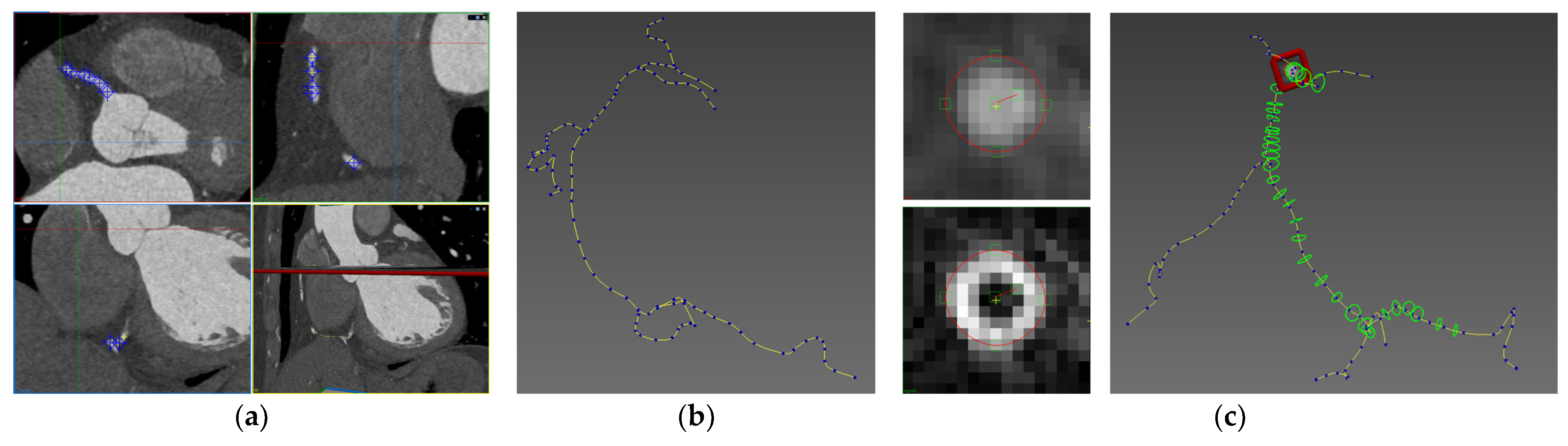
Firstly, the centerline of each branch was drawn as a set of points, from which the segmentation began, layer-by-layer (Figure 1a). A total of 40 to 60 control points were typically required to define the full RCA main branch, depending on individual vessel length and curvature, and particular care was taken in stenotic regions, critical for later FFR estimation (Figure 1b). Afterwards, a sequence of equally spaced cross-sectional planes was automatically generated perpendicular to the previously defined centreline, allowing the user to select the respective cross-sectional area occupied by blood in each plane. The segmentation was performed using the software’s Spline Polygon Tool, in which the user delineates the lumen contour by placing control points along the inner wall of the vessel (Figure 1c). The segmentation was conducted with close reference to the contrast-enhanced lumen visible in each CCTA slice.

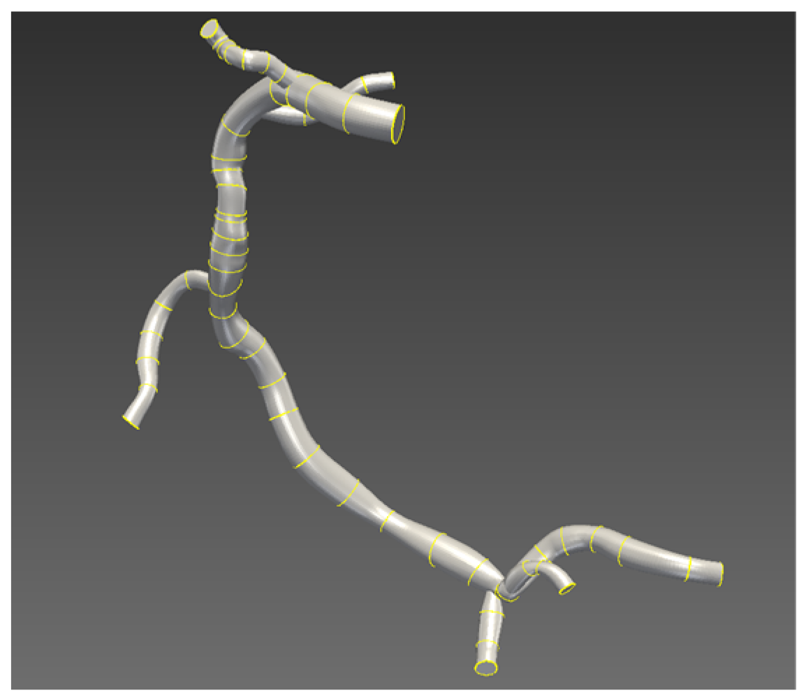
The model was then lofted using the drawn layers as a guideline, resulting in a 3D representation of the resting lumen vessel, a state under which all patients performed the imaging exams. This lofting process relies on the discretisation of each contour using a fixed number of sampling points to define the surface mesh resolution along the circumference [21]. Every patient’s final geometry was reconstructed with >40 sampling points, avoiding lofting failures while preserving anatomical fidelity in the reconstructed model, as seen in Figure 2 below.

Hyperemic Scaling Conditions and Assumptions

For an accurate estimation of non-invasive FFR, it is essential that the simulations reproduce the maximal vasodilation conditions under which the invasive FFR is clinically defined. In practice, such conditions are induced by the intravenous administration of a pharmacologic vasodilator, typically adenosine, which provokes systemic and coronary responses that closely mimic those observed during physical stress or exercise. Experimental studies in humans have shown that adenosine infusion leads to a reduction in mean arterial pressure of approximately 6 mmHg, an increase in heart rate of around 24 bpm, and a 4.4-fold increase in absolute myocardial blood flow, primarily due to a 4.17-fold reduction in microvascular resistance [22].

In computational models, these hemodynamic adjustments can be introduced by scaling the resting-state parameters accordingly. Following the framework proposed by Sharma et al. (2012), hyperemic conditions are derived from the resting state through a transfer relation that decreases outlet resistances to reflect drug-induced vasodilation [23]. In the present work, this was implemented by applying a fixed scaling factor of 2.04 across the cross-sectional area of the whole RCA lumen. This factor ensures that the relative reduction in vascular resistance (proportional to the inverse of the fourth power of radius) is consistent with the expected physiological drop during maximal hyperemia. The resulting setup yields flow and pressure distributions representative of adenosine-induced hyperemia, providing a physiologically sound reference for FFR computation.

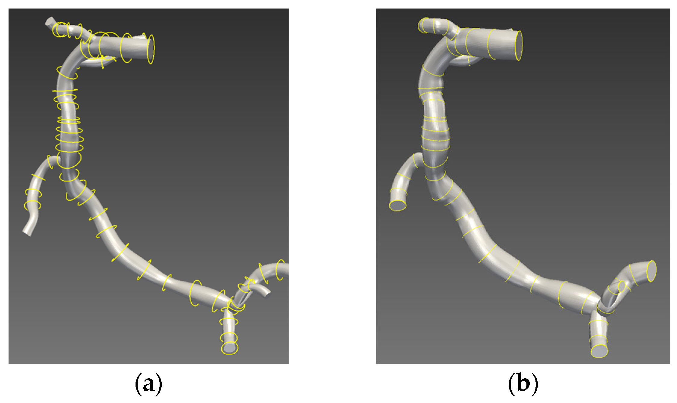
The previously mentioned parameters were included either in the geometric model itself or in the data analyzed afterwards for the User-Defined Functions (UDFs). SimVascular allows for the insertion of user-created scripts in order to answer this request, and this capability was a decisive factor in choosing SimVascular as the segmentation tool in this workflow. An open-source Python script 3.12.7 was designed for that end. This script was able to scale the cross-sectional contours of each segmentation plane by a factor of 2.04 in area, as seen in Figure 3a. Figure 3b shows the final RCA model after the hyperemic transformation.

Following the hyperemia establishment, localized smoothing was applied to the geometries to remove surface irregularities and abrupt transitions from the RCA main branch to the secondary branches. Smoothing was performed selectively by the user, avoiding excessive editing to preserve anatomical detail, while ensuring good quality surfaces that would not affect flow predictions in CFD simulations.

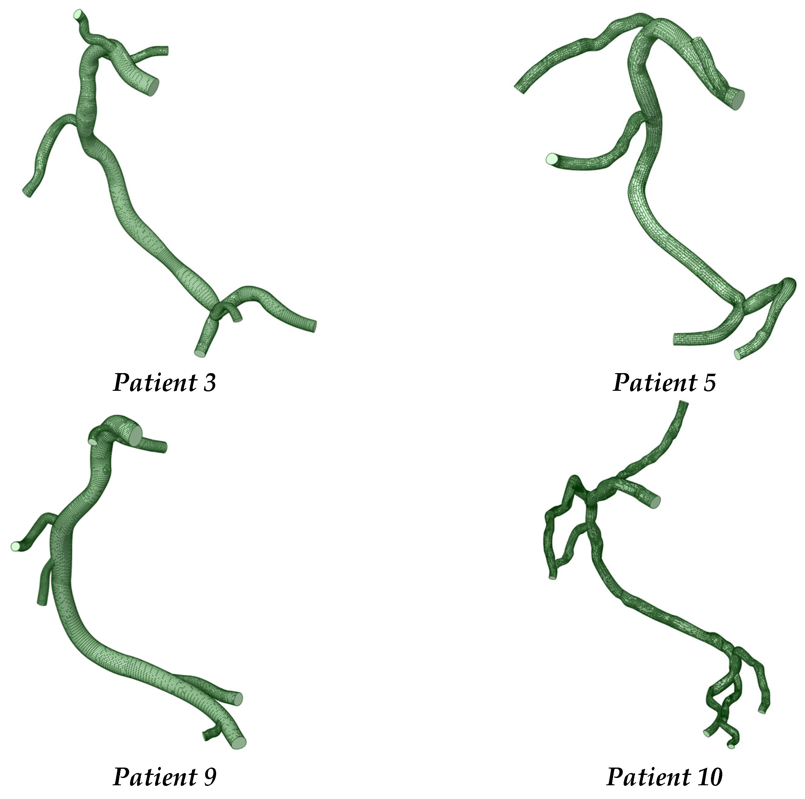
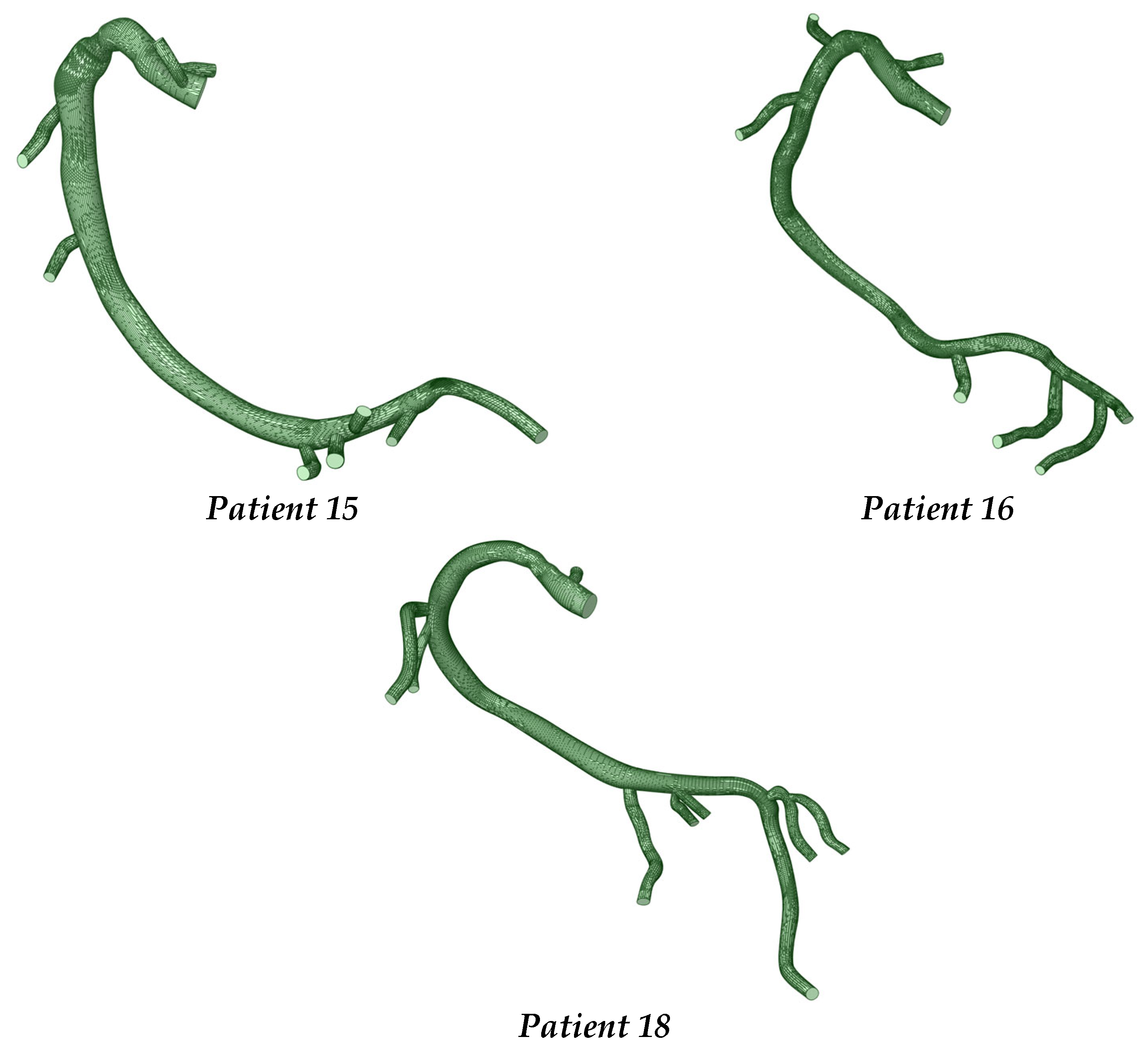
All geometries were then imported to ANSYS SpaceClaim^® 2025R1, where final operations such as orientation and named selections were performed. All the reconstructed RCAs in the hyperemic state can be viewed in Figure 4.

2.3. Meshing

Accurate mesh generation is a critical step in CFD-based coronary simulations since the correct prediction of pressure drops depends heavily on local mesh resolution. Insufficient refinement or poor-quality elements can introduce numerical diffusion and lead to significant errors in pressure-derived indices such as FFR [8].

To identify the most robust meshing strategy for patient-specific RCA geometries, different workflows were tested in ANSYS^® 2025R1 software, including the standard Meshing module, the Watertight Geometry Workflow in Fluent Meshing, and the Fault-Tolerant Meshing (FTM) pipeline. The complex and detailed morphology of STL-based coronary models derived from SimVascular caused the conventional methods to fail or yield meshes with high skewness and non-uniform element sizes, which led to unstable results.

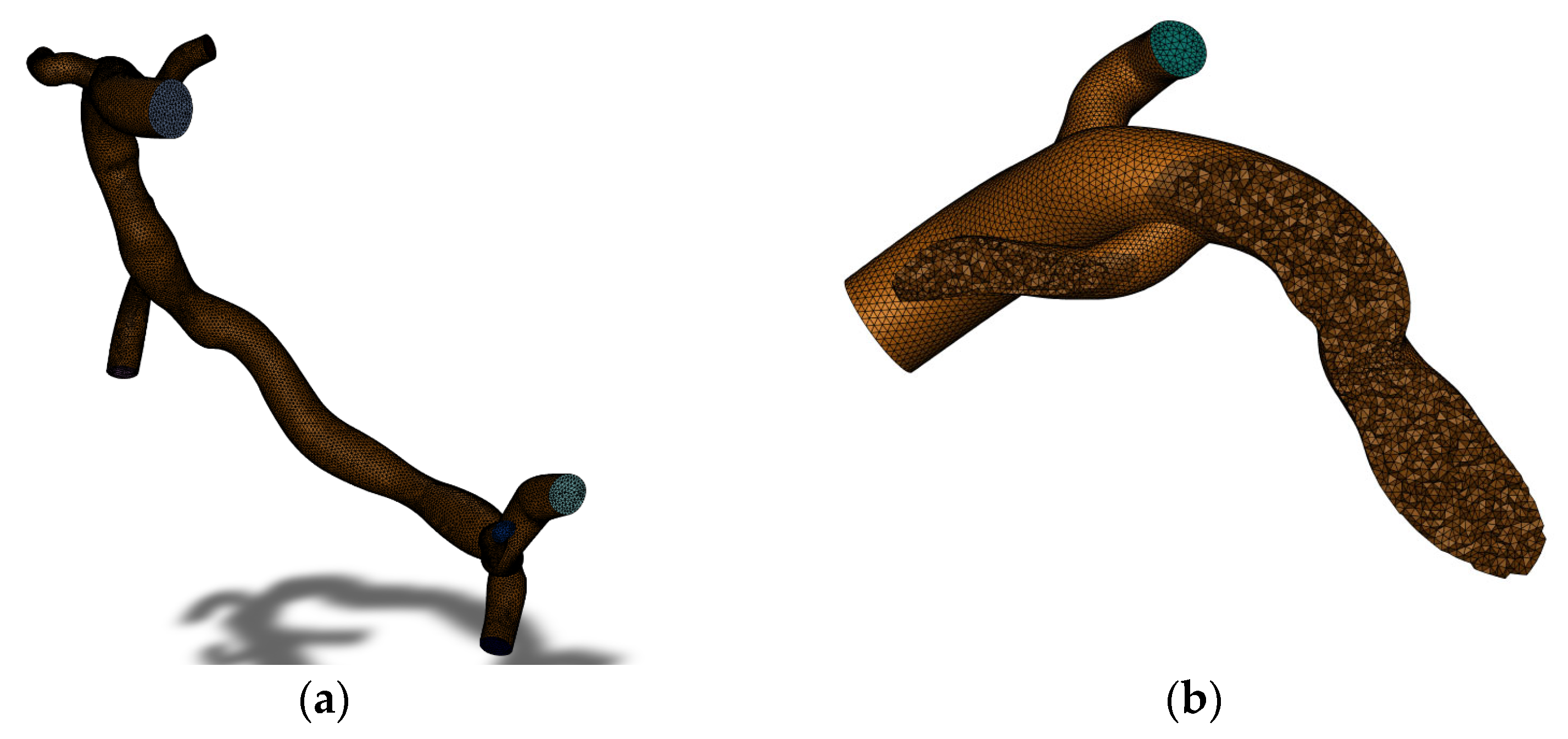
The FTM workflow was therefore adopted for all models (Figure 5). Designed to handle faceted and irregular surfaces, FTM generated high-quality, non-conformal tetrahedral meshes that maintained geometric fidelity. In this setup, element sizes were uniformly constrained between 0.3 and 0.4 mm, providing consistent resolution and minimizing abrupt transitions across the lumen. Mesh quality was monitored using skewness, which was required to remain below 0.7.

Given the clinical focus of the present study, the meshing strategy was designed to ensure numerical robustness while preserving clinical feasibility and computational efficiency. Based on prior experience and conclusions reported in previous coronary artery CFD studies, mesh convergence has been consistently observed to be achieved at approximately 300,000 elements [12]. To ensure that all simulations were performed well within this mesh-stable regime, patient-specific meshes were intentionally oversized, with initial mesh sizes ranging between 800,000 and 900,000 elements for all cases.

In addition, adaptive mesh refinement was applied using the solver’s dedicated refinement tool, targeting regions exhibiting the highest pressure gradients, segments that are critical for FFR computation, resulting in around 1,000,000 cell meshes for all patients. This procedure ensured that the resulting FFR values remained stable and consistent with the previous simulation for each patient.

2.4. Blood Rheological Model

In this study, blood was modeled as a non-Newtonian viscoelastic fluid using a multi-mode implementation of the simplified Phan-Thien/Tanner (sPTT) model (see Appendix A). This approach was chosen to capture the complex rheological behavior of blood, especially in the microcirculation and in regions with disturbed flow patterns such as stenoses and bifurcations, where the viscoelastic nature of blood becomes significant [12].

The sPTT model is used for modeling shear-thinning and viscoelastic effects in complex fluids. Its implementation in ANSYS Fluent^® was achieved via User Defined Functions (UDFs), where four viscoelastic modes were defined, each with its own characteristic relaxation time (λ), extensibility parameter (ε), and elastic viscosity component (μₑ). The total extra stress tensor is computed as the sum of the contributions from all four modes. The general form of the stress evolution equation for each mode is as follows:

$${\displaystyle \frac{\partial T_n}{\partial t}}+u·\nabla T_n-{\left(\nabla u\right)}^T·T_n-T_n·\nabla u={\displaystyle \frac{{\mathrm{\mu }}_{e,n}}{{\mathrm{\lambda }}_n}}\left(\nabla u+\nabla u^T\right)-{\displaystyle \frac{1}{{\mathrm{\lambda }}_n}}\hspace{0.17em}f\left(\mathrm{tr}\left(T_n\right)\right)\hspace{0.17em}{T}_n$$

(1)

where $T_n$ is the extra stress tensor of mode n, ${\mathrm{\lambda }}_n$ is the relaxation time, ${\mathrm{\mu }}_{e,n}$ is the elastic viscosity, and $f\left(\mathrm{tr}\left(T_n\right)\right)=1+{\displaystyle \frac{{\mathsf{ϵ}}_n{\mathrm{\lambda }}_n}{{\mathrm{\mu }}_{e,n}}}\hspace{0.17em}\mathrm{tr}\left(T_n\right)$ is the stress coefficient function accounting for extensibility.

The formulation solves additional transport equations for the extra stress tensor components, incorporating their source terms directly into the momentum equations. This approach enables the simulation of both shear-thinning and time-dependent viscoelastic effects under pulsatile flow. Such modeling is particularly relevant for coronary hemodynamics, where these rheological responses influence local pressure gradients and wall shear stresses, ultimately improving the physiological accuracy of computed FFR.

The fitting of this model’s parameters was inspired by the previous work on blood viscoelasticity performed by Campo-Deaño et al. (2014), with included critical details analyzed by Good et al. (2016) and Bodnár et al. (2011), who highlighted that viscoelasticity effects should not be neglected [24,25,26].

2.5. Boundary Conditions

The accurate representation of boundary conditions is a critical factor in coronary CFD simulations, directly influencing the realism and clinical relevance of the predicted hemodynamic metrics. In this methodology, a Womersley model was implemented at the inlet to obtain a patient-specific pulsatile flow pattern that mimics physiological behavior, whereas at the outlet, a three-element Windkessel model simulated the realistic microenvironment present at the distal regions of the RCA geometries.

2.5.1. Inlet Boundary Condition–Womersley Model

To reproduce realistic pulsatile coronary flow, the inlet velocity of each model was defined using a Womersley velocity profile, which analytically describes oscillatory flow in a rigid cylindrical tube. This formulation accounts for the frequency-dependent attenuation of flow oscillations across the vessel cross-section and captures the temporal and radial velocity distribution more accurately than steady or parabolic profiles, particularly in low Womersley-number vessels such as coronary arteries [27].

The profile was reconstructed through a Fourier-based velocity waveform combining multiple harmonic components derived from patient-specific cardiac cycle data. Input parameters included the vessel inlet radius, heart rate, cardiac period, and the respective Womersley number. The resulting transient velocity field dynamically evolves throughout the simulation, ensuring that inlet pulsatility and amplitude match physiological conditions representative of each patient’s coronary circulation.

Mathematically, the velocity at a given radial position $r$ and time $t$ is computed using the following expression:

$$u\left(r,t\right)=A_0\left(1-{\left(r/R\right)}^2\right)+\sum _{k=1}^{N}R\left\{\left[A_k-i{B}_k\right]e^{i{\omega }_{k}t}\left(1-{\displaystyle \frac{J_0\left({\alpha }_{k}r/R\right)}{J_0\left({\alpha }_k\right)}}\right)/\left(1-{\displaystyle \frac{2J_1\left({\alpha }_k\right)}{{\alpha }_k{J}_0\left({\alpha }_k\right)}}\right)\right\}$$

(2)

where $J_0$ and $J_1$ are Bessel functions of the first kind (orders 0 and 1), ${\alpha }_k=\alpha \sqrt{k}$ is the harmonic-specific Womersley number, ${\mathrm{\omega }}_k=2\mathrm{\pi }k/T$ is the angular frequency for harmonic $k$, $A_k$ and $B_k$ are the cosine and sine Fourier coefficients for harmonic k, and R is the radius of the vessel (see Appendix A).

2.5.2. Outlet Boundary Condition–3-Element Windkessel Model

At each coronary outlet, a 3-element Windkessel model (WK3) was applied to represent the interaction between the coronary arteries and the distal microcirculation. This LPM captures both the resistive and capacitive effects of the downstream vasculature, enabling realistic pressure–flow coupling without explicitly modeling the entire circulatory network (see Appendix A).

The model includes a proximal resistance (R_p) for large-artery impedance, a compliance (C_a) representing arterial wall elasticity, and a distal resistance (R_d) that characterizes microvascular resistance. These parameters dynamically update at every time step according to the local outlet flow and pressure, ensuring transient consistency with the cardiac cycle:

$$R_p=0.09·{\displaystyle \frac{A_i}{A_{\mathrm{tot}}}}·R_{\mathrm{tot}}$$

(3)

$$R_d=0.91·{\displaystyle \frac{A_i}{A_{\mathrm{tot}}}}·R_{\mathrm{tot}}$$

(4)

$$C_a={\displaystyle \frac{A_i}{A_{\mathrm{tot}}}}·C_{\mathrm{tot}}$$

(5)

A_i represents the cross-sectional area of the outlet branch i, C_tot the total compliance, and R_tot the total vascular resistance.

Patient-specific physiological data, such as outlet area, total vascular resistance, and total compliance, were used to scale the Windkessel parameters proportionally across all branches. This ensured that the downstream boundary response reflected each patient’s unique coronary geometry and flow distribution, allowing physiologically accurate pressure recovery and waveform propagation within the CFD domain.

The whole pipeline for the Windkessel model implementation follows the established procedure described by Deyranlou et al. (2020) and Werternhof et al. (2009) [28,29].

2.6. Numerical Settings

All simulations were performed using the ANSYS Fluent^® solver, selected since its post-processing features allow for high-quality result visualization and understanding, as shown by our previous studies [12,30]. The SIMPLE algorithm was used to solve the equations of this unsteady, incompressible, and pulsatile flow. Second-order spatial and temporal discretization schemes were adopted to minimize numerical diffusion when implementing all UDFs. A time-step of 0.005 s, with 20 iterations per time-step, was adopted in order to balance accuracy with computational cost. For each patient, 3 to 5 full cardiac cycles were simulated, depending on cycle duration, and all extracted values correspond to the last full cardiac cycle available for analysis. The cardiac cycle duration was individually estimated based on the frequency used for the Womersley inlet condition. For each simulation, the correspondence of each user-defined scalar (UDS) in the fluid’s source terms and scalar’s mass flow rate was established in order to correctly couple the constitutive equations of the sPTT model with the momentum equations during the simulation.

Convergence was monitored through two complementary approaches: numerical convergence of the viscoelastic stress equations was targeted at a residual threshold of 10⁻⁶, and physiological convergence was verified by ensuring that the final 2–3 cardiac cycles presented stable waveforms in three key area-weighted surface monitors (aortic pressure, distal pressure, and inlet velocity).

Due to the coupling between the boundary condition models and the blood rheology formulation, a two-step simulation procedure was required to achieve physiologically consistent results.

The first simulation was designed to determine the mean inlet flow rate ($\mathrm{C}$), which served as an input for initializing the WK3 UDF in the final simulation. The sPTT rheology was activated alongside the pulsatile Womersley UDF at the inlet, while all outlets were assigned a zero-pressure condition. This configuration allowed the flow distribution to depend solely on the geometry and inlet waveform, isolating the intrinsic hemodynamic behavior of each model. This step includes the editing of each patient’s Womersley UDF with the respective data, both measured in the hospital and present in the respective reconstructed geometry, such as the heart rate (adapted for hyperemia by adding 24 BPM), cardiac cycle duration, and inlet area, which leads to obtaining the Womersley number.

Once a periodic state was achieved, the velocity waveform at the inlet was sampled over the last complete cardiac cycle. The mean velocity was then obtained using the trapezoidal integration rule.

The computed mean velocity was multiplied by the inlet cross-sectional area to obtain the mean volumetric flow rate, which was subsequently used as input for calibrating the WK3 outlet model in the second, fully coupled simulation.

This final simulation incorporated the complete set of physiological boundary conditions and aimed to compute the non-invasive FFR. Using the flow data and mean inlet velocity obtained from the preliminary run, the WK3 model was now employed at each outlet to capture the resistive and capacitive effects of the coronary microcirculation. Both Womersley and sPTT UDFs remained active.

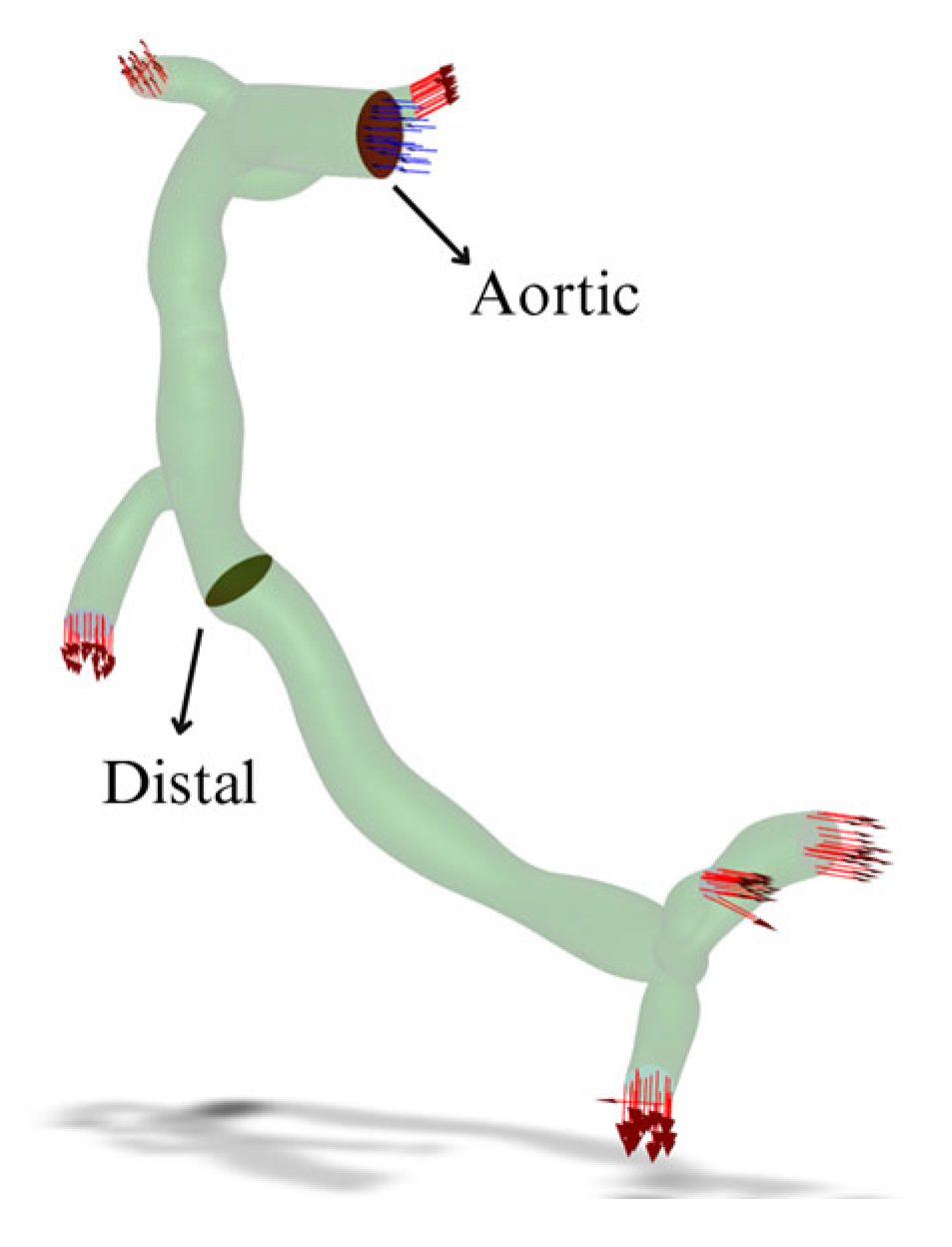
During the transient simulation, pressure data were recorded at two planes: one located at the inlet region, the aortic plane, and another 20 mm downstream of the stenosis, mimicking the clinical measurement sites used in invasive FFR assessment. Figure 6 shows this operation.

The spatial and time-averaged pressure at each plane was tracked by the solver for multiple cardiac cycles. The values from the last full cycle were then integrated using the trapezoidal rule. The FFR was then computed as the ratio between the mean distal and proximal (aortic) pressures:

$$\mathit{FFR}={\displaystyle \frac{{\overline{P}}_{\mathit{distal}}}{{\overline{P}}_{\mathit{aorta}}}}$$

(6)

This procedure ensured that the calculated FFR reflected the hemodynamic significance of each stenosis, mimicking, at best, physiological conditions, under a patient-specific flow.

Given the proprietary nature of HeartFlow^®, no information regarding internal boundary conditions, hyperemic modeling, or distal pressure sampling location was available, and comparisons were therefore limited to reported FFR outputs.

All simulations were performed on a local workstation (AMD Ryzen 9 7950X, 128 GB RAM, Advanced Micro Devices, Santa Clara, CA, USA). Each final patient-specific transient simulation under hyperemic conditions required approximately 10 h.

3. Results and Discussion

In this section, the results obtained for all patients will be presented and discussed, involving all the acquired data from the simulations. Velocity and pressure contours were captured during systolic and diastolic peaks to analyze differences in blood-flow behavior. This visualization allows identification of areas with high shear and flow acceleration proximal to stenoses, as well as abrupt pressure drops that significantly alter the FFR. Then, the non-invasive FFR results will be compared with the values obtained invasively and by HeartFlow^®.

3.1. Velocity Contours

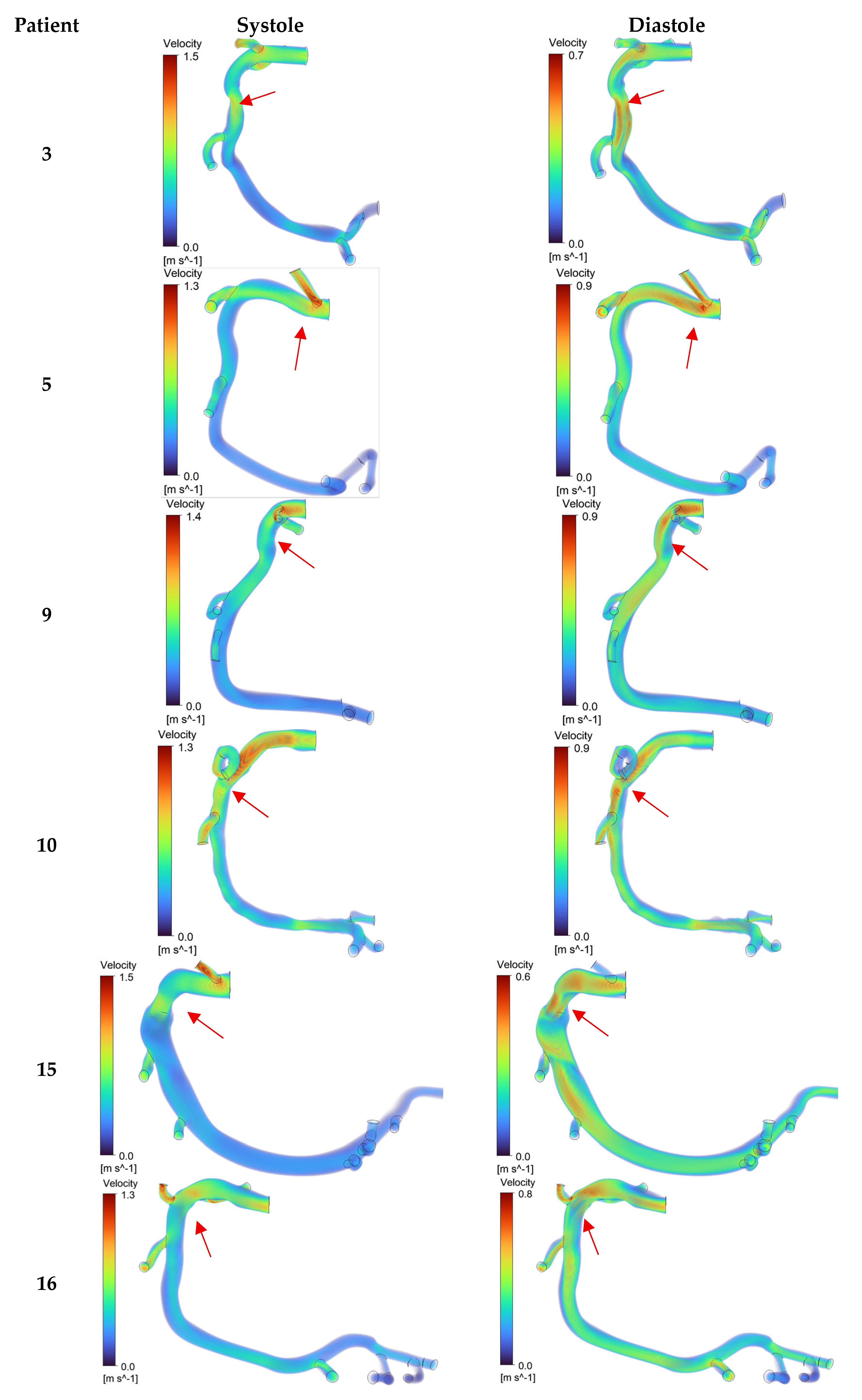
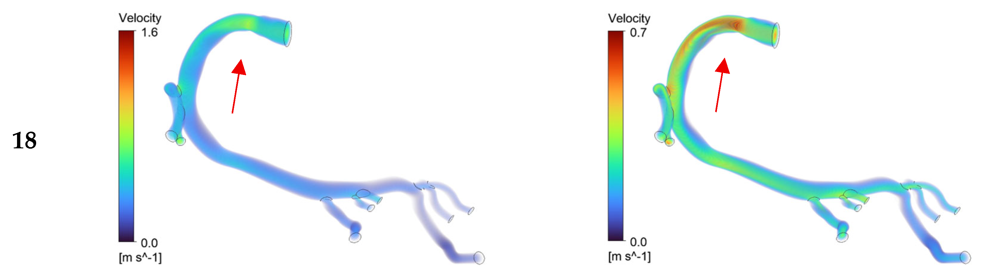
Velocity contours were captured during systolic and diastolic peaks in order to analyze differences in blood-flow behavior. The results reveal consistent physiological patterns across all patients and both time points of the cardiac cycle. As expected, peak velocities occur during systole, when ventricular contraction generates an increased coronary flow. Figure 7 shows the obtained contours for all patients.

Across the hyperemic RCA geometries, localized accelerations are observed downstream of the stenoses, with sharp velocity gradients. The regions upstream and downstream of each lesion display well-defined transition zones where velocity magnitude decreases rapidly, reflecting the pressure recovery process. Patients with more severe luminal narrowing, such as Patients 3 and 10, exhibit systolic peak velocities of approximately 1.4–1.5 m/s, supporting the chance for functionally relevant stenoses. In contrast, smoother velocity distributions are seen in less stenotic cases, such as Patients 5 and 16, with peak velocities typically ranging between 0.7 and 0.9 m/s, indicating reduced hemodynamic impact.

The diastolic phase shows a general reduction in velocity magnitude and a more uniform flow distribution, consistent with the lower driving pressure during ventricular relaxation. Average diastolic velocities in the main RCA branch range between 0.35 and 0.55 m/s, approximately 40–60% lower than systolic peaks, reflecting the reduced pressure gradient in this stage. Despite the drop in velocity magnitude, persistent flow acceleration and directional asymmetry can still be identified near the stenoses, where velocity increases of up to 0.3 m/s are observed in multiple patients. This velocity profile demonstrates that even during low-pressure phases, this CFD approach can help in accurately detecting functionally limiting lesions.

Overall, the velocity field evolution under hyperemia clearly delineates the influence of coronary geometry on local flow behavior. The described patterns are physiologically coherent and align with expected coronary dynamics under maximal vasodilation, supporting the validity of the simulated flow regime used for FFR computation.

3.2. Pressure Contours

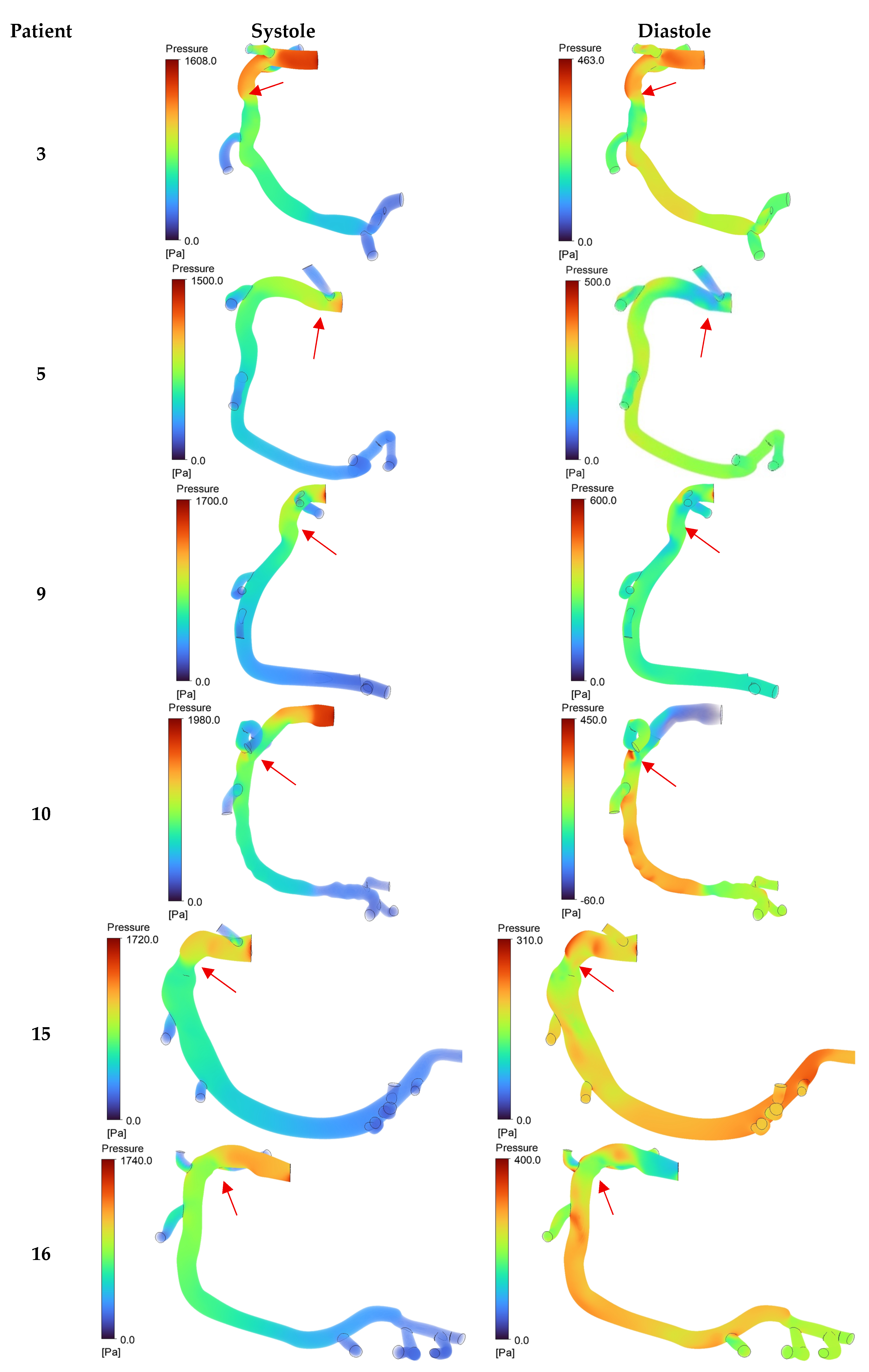
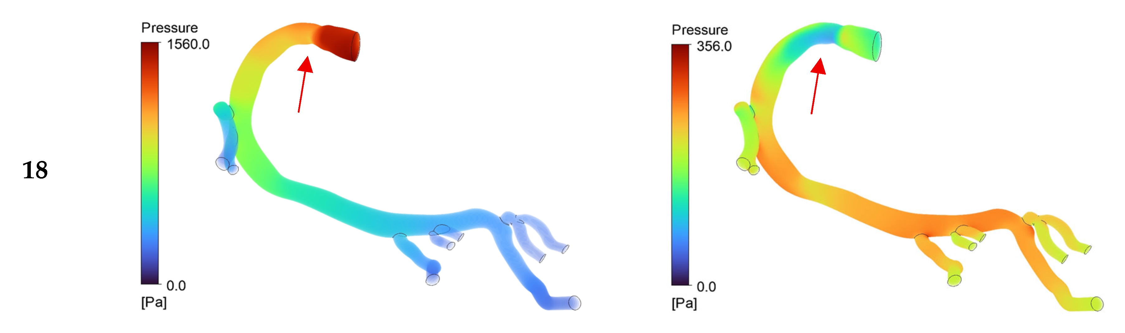
The obtained pressure contours reveal distinct patterns between systolic and diastolic phases, providing valuable insights into the hemodynamic significance of each stenosis. As expected, systolic pressures are consistently higher, with inlet values typically exceeding 1600 Pa upstream of the stenosis, reflecting the elevated driving force generated during ventricular contraction and the increased flow demand under maximal vasodilation. The respective contours for all patients are shown in Figure 8.

Pronounced pressure drops are clearly observed across stenotic regions, particularly in Patients 3, 10, and 18, where the lumen narrowing is most noticeable. These abrupt gradients mark the areas of greatest resistance to flow and correspond to the functionally significant lesions.

During diastole, overall pressure levels decrease as the driving gradient diminishes, yet the spatial distribution remains consistent with the systolic phase. In this cardiac stage, pressures near the aortic inlet range between 150 and 300 Pa, showing the accurately simulated difference between the systolic phase.

The resulting distributions align closely with physiological expectations: a steep proximal-to-distal pressure decay during systole and a less significant behavior during diastole. These findings confirm that the simulated flow and pressure fields accurately reproduce coronary hemodynamics under hyperemia, supporting their use in non-invasive FFR estimation and patient-specific assessment of stenosis severity.

The post-stenotic flow behavior observed in the present patient-specific simulations is consistent with classical numerical studies conducted in idealized stenosed geometries. Previous investigations have reported strong flow acceleration at the stenosis throat, followed by flow separation, the formation of recirculation regions downstream, and a marked pressure drop across the constriction. Moreover, these studies indicate that such effects become increasingly pronounced for stenosis severities above approximately 50–70% area reduction, leading to longer recirculation zones and higher wall shear stress peaks near the throat [31,32]. The velocity and pressure fields obtained in the present three-dimensional coronary simulations qualitatively reproduce these well-established hydrodynamic patterns, while extending them to anatomically realistic right coronary arteries under physiological flow conditions.

3.3. Non-Invasive FFR vs. Invasive FFR

To assess the accuracy of the proposed computational framework, the non-invasive CFD-derived FFR values were compared with both invasive wire-based FFR (taken as the reference standard) and HeartFlow^® (an already implemented alternative) results under hyperemic conditions.

Table 2. Invasive and HeartFlow^® FFR values compared with the obtained non-invasive FFR.

Patient	Invasive FFR	HeartFlow® FFR	Non-Invasive CFD FFR	Relative Error: Non-Invasive vs. Invasive
3	0.68	0.56	0.64	5.9%
5	0.90	0.92	0.86	4.4%
9	0.93	0.91	0.91	2.2%
10	0.75	0.82	0.77	2.7%
15	0.76	0.92	0.68	10.5%
16	0.97	0.96	0.81	16.5%
18	0.89	0.93	0.74	16.9%
Average	-	-	-	8.4%

presents these, including the respective relative error.

Across the patient dataset, the computed non-invasive FFR values demonstrated a strong agreement with the invasive measurements, with relative errors ranging from 2.2% to 16.9%. Five of seven patients showed deviations below 11%, and four within 6%, confirming the pipeline’s reliability while being entirely built on open-source segmentation and user-defined modeling functions. This level of accuracy highlights the robustness of the workflow and the consistency achieved through its physiologically realistic model implementations.

Patients 9, 5, and 10 showed the best correspondence, with relative errors of 2.2%, 4.4%, and 2.7%, respectively. In all three cases, the CFD-predicted FFR values reproduced the correct clinical classification of each lesion relative to the diagnostic threshold of 0.80. Patient 3 also exhibited a coherent result, with an FFR of 0.64 versus 0.68 invasively, both indicating a functionally significant stenosis, requiring additional medical intervention. These cases illustrate the method’s capacity to accurately predict flow-limiting lesions across different degrees of narrowing.

Larger discrepancies were observed for Patients 16 and 18, where the model underestimated the invasive FFR by 16.5% and 16.9%, respectively. These results would translate into Patient 18 being misdiagnosed regarding the 0.80 threshold, being the only patient in that scenario for the whole dataset. Potential sources of deviation include inherent limitations in capturing patient-specific microvascular response, either because of software restrictions or due to user-dependent segmentation.

Overall, the results indicate that the non-invasive CFD-based approach tends to slightly underestimate FFR compared with invasive measurements, a trend consistent with previously reported computational studies. This slight systematic underestimation may reflect the combined effect of viscoelastic blood modeling and physiologically calibrated Windkessel boundary conditions, which tend to increase distal pressure losses compared with simplified or wire-perturbed invasive measurements. During the invasive procedure itself, the presence of the pressure guidewire can slightly elevate downstream resistance and disturb the blood flow, leading to artificially higher FFR readings. Therefore, the lower CFD-predicted values are expected, while presenting a good agreement with the gold standard technique.

These findings reinforce that the proposed non-invasive framework can achieve clinically meaningful FFR values with high fidelity under hyperemic conditions, while maintaining full methodological transparency. Minor underestimations, though present, remain within acceptable diagnostic margins and primarily reflect differences in measurement approach rather than fundamental model error.

3.4. Non-Invasive FFR vs. HeartFlow^®

To further contextualize the accuracy of the proposed CFD-based pipeline, its results were compared against HeartFlow^® values and the invasive FFR reference standard.

Table 3. Comparison of the obtained relative errors between both Heartflow^® and the proposed CFD pipeline against the reference invasively acquired values.

Patient	Relative Error: Non-Invasive CFD vs. Invasive	Relative Error: HeartFlow® vs. Invasive
3	5.9%	17.6%
5	4.4%	2.2%
9	2.2%	2.2%
10	2.7%	9.3%
15	10.5%	21.1%
16	16.5%	1%
18	16.9%	4.5%
Average	8.4%	8.3%

summarizes the relative errors of both non-invasive approaches when evaluated against the invasive benchmark.

Across the studied sample, the proposed CFD method achieved an average relative error of 8.4%, comparable to HeartFlow^®’s 8.3%. Despite this marginal numerical difference, the clinical implications are significant. While the CFD model would have misclassified only one patient (Patient 18), HeartFlow^® misclassified two cases (Patients 10 and 15), one due to underestimation and the other due to overestimation of FFR, with a maximum error of 21% against the invasive. In particular, HeartFlow^®’s prediction for Patient 15 (0.92 vs. 0.76 invasive) would have led to an incorrect classification of a flow-limiting stenosis as non-significant, representing a clinically relevant misdiagnosis.

Both non-invasive techniques show small deviations relative to invasive values. However, the CFD pipeline demonstrates greater consistency, with a lower standard deviation of 6.3% compared to 8.1% for HeartFlow^®. Most importantly, this level of precision was achieved using a fully transparent, reproducible, and open-source framework, free from proprietary components or undisclosed algorithms. In contrast to HeartFlow^®, which remains a high-cost, black-box system, the proposed CFD pipeline allows full control of each computational stage, facilitating continuous refinement and promoting benchmarking, as well as academic and clinical reproducibility.

In summary, both HeartFlow^® and the developed CFD pipeline yield reasonably accurate FFR estimations. Yet, the CFD model stands out by offering complete transparency, reproducibility, flexibility, and clinical interpretability. Operating entirely under open-source principles, it achieves comparable diagnostic performance with fewer misclassifications, highlighting its potential as a cost-effective alternative for non-invasive coronary physiology assessment.

4. Conclusions

By explicitly addressing previously reported limitations related to model simplification, transparency, and right coronary artery applicability, this study presented and validated a fully transparent CFD-based computational pipeline for the non-invasive estimation of FFR in patient-specific RCAs. The workflow integrates CT-based 3D reconstruction, hyperemic scaling, fault-tolerant meshing, Womersley inlet profiles, three-element Windkessel outlet models, and a viscoelastic sPTT blood rheology formulation. The obtained non-invasive FFR values were systematically compared against invasive wire-based measurements and HeartFlow^® results, demonstrating that the proposed methodology effectively translates these modeling choices into clinically relevant functional assessment, while addressing past approaches’ limitations. The proposed open-source methodology successfully enabled reconstruction, meshing, and simulation of all patient-specific RCA geometries with stable hemodynamic convergence and high anatomical fidelity.

The computed FFR values showed good agreement with invasive measurements, with a mean relative error of 8.4%. Only one case (Patient 18) yielded a misclassification relative to the 0.80 clinical threshold, which represented fewer clinically relevant discrepancies than those obtained by HeartFlow^®. These results confirm that the pipeline can accurately reproduce the hemodynamic impact of coronary stenoses while maintaining full methodological transparency and adaptability.

Future work will focus on improving the proposed framework along two main directions: workflow automation and broader clinical validation. The vessel segmentation process, due to being manually performed in SimVascular, represents the most time-consuming and user-dependent step, which could be replaced with automatic or semi-automatic alternatives in the future. However, SimVascular allows for automatic hyperemia transformation, unlike other commercial semi-automatic available software, translating into a good asset for anatomical identity. In parallel, extending the validation of the methodology to additional coronary branches, such as the left coronary arteries, will be essential to further assess the generalizability and clinical robustness of the proposed approach, although the availability of matched CCTA and invasive FFR data remains clinically constrained. In summary, this work demonstrates that a non-invasive, CFD-based FFR estimation framework can achieve clinically relevant diagnostic accuracy for RCAs. By offering an open, transparent, and cost-effective alternative to commercial platforms, this framework provides a credible foundation for integrating CFD-based FFR estimation into clinical workflows.