Article

A Graphical Approach to the Generalized Extremal Problem of a Transported Log in a Navigable Canal

Department of Mathematics, Faculty of Natural Sciences and Informatics, Constantine the Philosopher University in Nitra, Tr. A. Hlinku 1, 949 01 Nitra, Slovakia
Mathematics 2026, 14(2), 386; https://doi.org/10.3390/math14020386
Submission received: 6 December 2025 / Revised: 11 January 2026 / Accepted: 19 January 2026 / Published: 22 January 2026
(This article belongs to the Section E1: Mathematics and Computer Science)

Abstract

This article presents the solution to an optimization problem concerning the longest wooden log that can be floated through two perpendicularly intersecting water canals. This application problem is further generalized and solved using a graphical method.

1. Introduction

The pursuit of optimal solutions is a frequent and compelling challenge encountered in applied contexts. Tihomirov [1] identifies several motivations for addressing extremal problems, including enhancing resource efficiency, the prevalence of extreme principles in natural laws, and combining human curiosity with our desire for comprehensive understanding.
The mathematical resolution of extremal problems relies on idealized models and established methodologies drawn from various mathematical disciplines, such as arithmetic, algebra, geometry, and calculus [2]. Furthermore, the engaging application content of these problems serves as a unifying factor for knowledge acquired across mathematics, technology, and other sciences. This article arose from an intriguing, applied problem derived from a well-known set of unsolved exercises used in advanced mathematics curricula at technical universities in the Slovak Republic. In this paper, we extend the original problem through mathematical generalization to create a practical application, which requires the use of graphical methods employed via dynamic geometry software.

2. Original Problem

The original extremal problem no. 469 is presented in ref. [3] (p. 113) as follows:
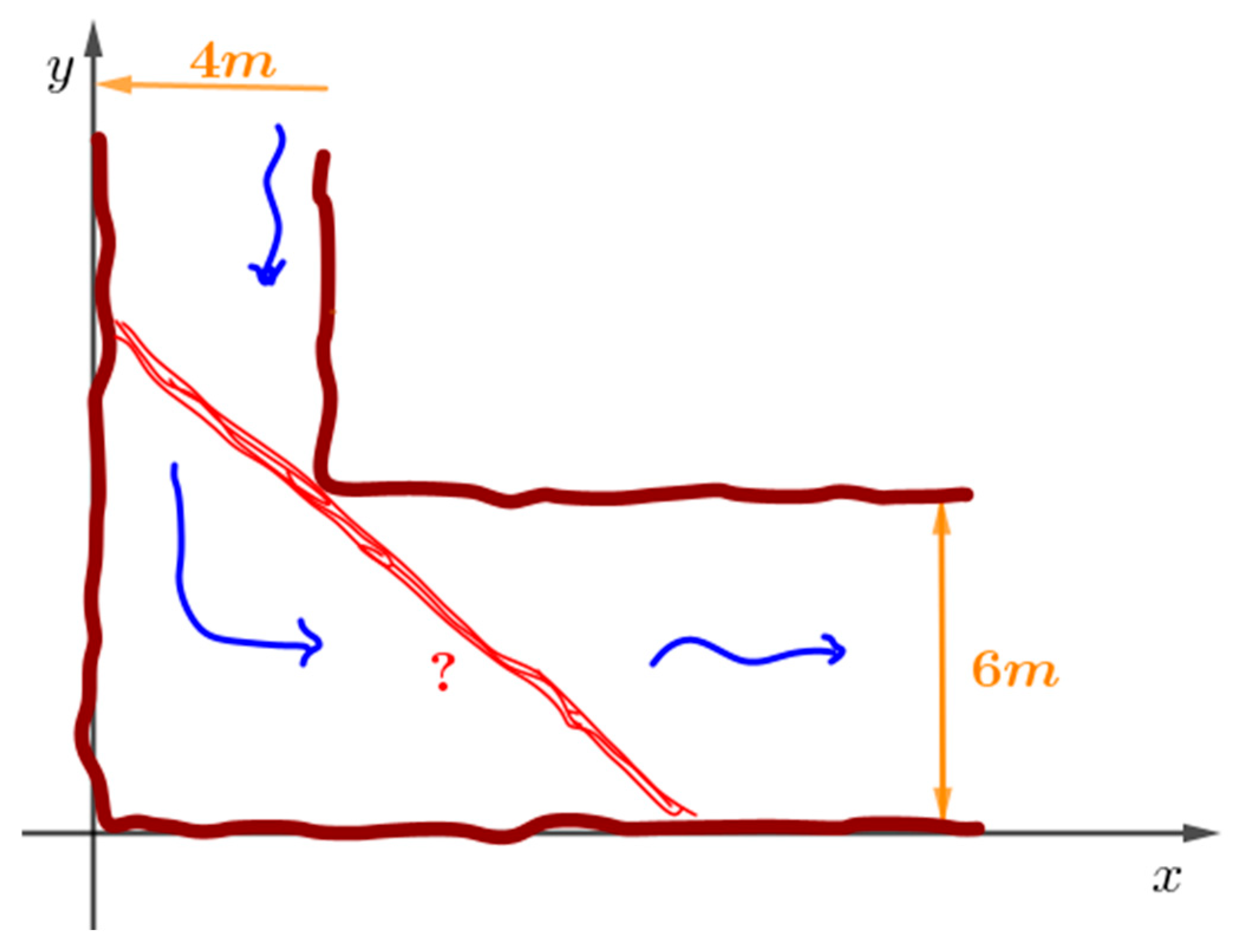
Two navigable canals that are perpendicular to each other have widths of 4 m and 6 m. Determine the maximum length of a log that can be floated through these canals (see Figure 1).
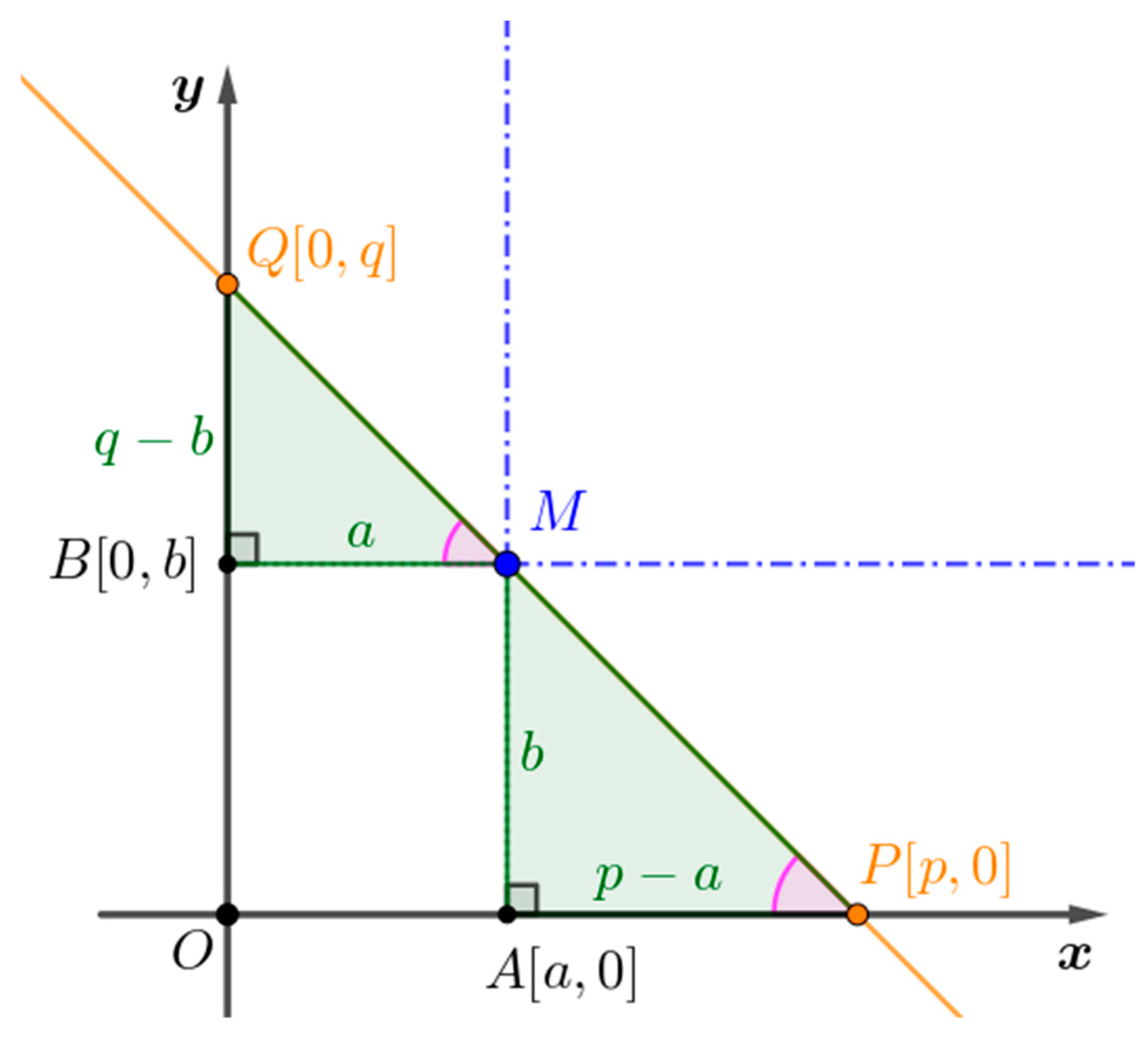
We consider the situation geometrically and in a general case. The model for the log is a line segment P Q defined by its endpoints P p , 0 and Q [ 0 , q ] , passing through a fixed point M [ a , b ] , for 0 < a b , a , b R .
The length P Q of the segment P Q is then defined using the Pythagorean theorem:
P Q = p 2 + q 2 .
Denoting A a , 0 , B 0 , b , the similarity of the triangles A P M and O P Q yields the following relation:
p a b = p q q = p b p a
for p R , p a (see Figure 2). Substituting Equation (2) into Equation (1) allows us to define the function F ( p ) of variable p :
F p = p p a · p a 2 + b 2 .
Next, we apply calculus methods to find the critical points (i.e., the values of the argument for which the first derivative has vanished or is discontinuous). We have
F p = p p a · p a 2 + b 2   F p = p p a 2 + b 2 a p a 2 p a 2 + b 2 .
A rule for testing a differentiable function y = F p for extremal values requires
F p = 0
and for us to find the real roots of this equation and the values of p at which the derivative F p becomes discontinuous (the first derivative is discontinuous at the point p 0 = a ).
We evaluate the critical points from Equation (4):
p 1 = a ,       p 2 = a + a b 2 3 ,
We now analyze the sign of the first derivative in the neighborhoods of the critical points.
If 0 < a   b , then it holds true that
0 < a < 2 a a + a b 2 3 < a + b .
We evaluate the values of the first derivative at the points x = 0 ,   x = 2 a , and x = a + b :
F 0 = 1 a a 2 + b 2 < 0 ,
F 2 a = = a 2 b 2 a a 2 + b 2 < 0 ,
F a + b = = a + b b 2 + a 2 > 0 .
This implies that the function y = F p decreases on the intervals , a a , a + a b 2 3 and increases on the interval a + a b 2 3 , . The function y = F p has its local minimum at the point x = p 2 .
Applying Equation (2), we calculate
q 2 = b + a 2 b 3 .
The corresponding points have the coordinates P 2 [ a + ( a b ^ 2 ) ,   0 ] ,   Q 2 [ 0 , b + ( a ^ 2   b ) ] . The lengths of the segments are equal:
P 2 Q 2 = = a 2 3 + b 2 3 3 2 .
Finally, we evaluate the point of discontinuity p 1 = a . For the value q 1 , we have
q 1 = lim p a p b p a = b · lim p a + p p a = = b · lim p a p p a = =
The line x = a is the asymptote of the function y = F x and passes through the point M a , b . However, this result does not represent a solution to the original problem.
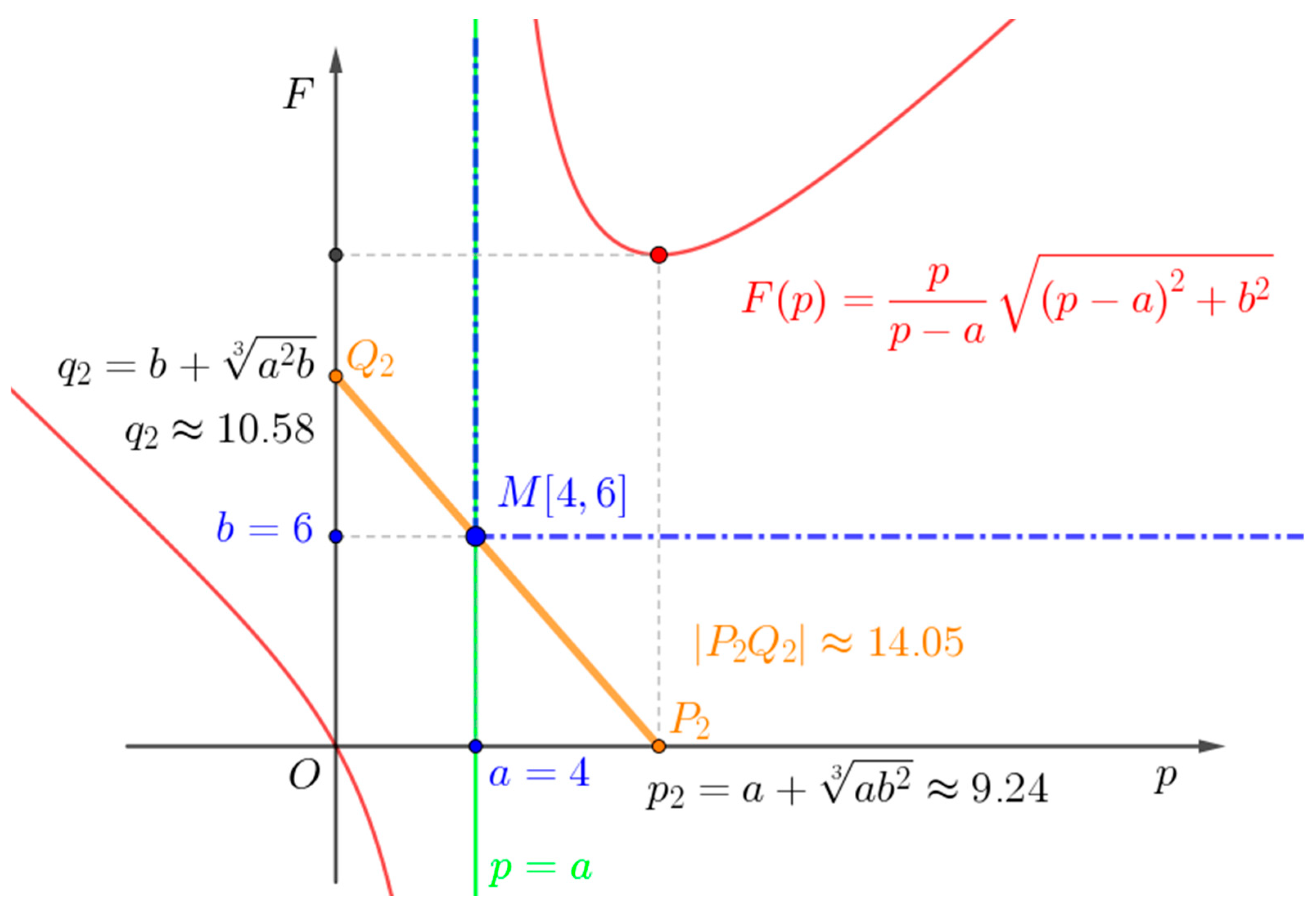
The correct solution to the original problem is provided by result (11) (see Figure 3).
Substituting a = 4 , b = 6 , we evaluate
P 2 Q 2 = = 4 2 3 + 6 2 3 3 2 14.05 m .
Remark 1.
This local minimum of the function corresponds to the maximum feasible length of a wooden log capable of traversing the rectangular navigable canals. Although the function F(p) attains a local minimum at this point, this minimum corresponds to the maximum feasible length of a log that can pass through the canals, since any longer log would violate the geometric constraints imposed by their widths.
Remark 2.
The resulting formula is “elegant” in terms of the powers that appear in it. As we will show later, the result is not random and corresponds to the geometric locus of points called astroids.

3. Generalized Extremal Problem

Formula (11) defines the log’s length as a function of the parameters a , b . However, if the wooden log is modeled as a rectangle of width r , result (11) is no longer applicable.
Consequently, we can now generalize the problem. In the following text, we assume linear canal boundaries, which will be defined by the coordinate axes and the respective rays. For the sake of clarity in the figures, these will be highlighted only in cases of the final visualization of specific application solutions.
Specifically, the original requirement concerning the line passing through the point M a , b is replaced by the condition involving the tangent line t to the graph of a function y = f x defined on an interval J 0 , .

Generalized Problem

Let a function y = f ( x ) be given, defined on an interval J , that satisfies the following assumptions:
(a)
The function y = f x   is non-negative on J .
(b)
The function y = f x   is continuous on the interval J .
(c)
The function y = f x   has continuous derivatives up to the 2 n d order, where f x 0 for x on J .
The tangent line t to the graph of the function y = f x at a point x 0 J intersects axes at points P p ,   0 and Q 0 ,   q . We determine the extremal length of the segment P Q .
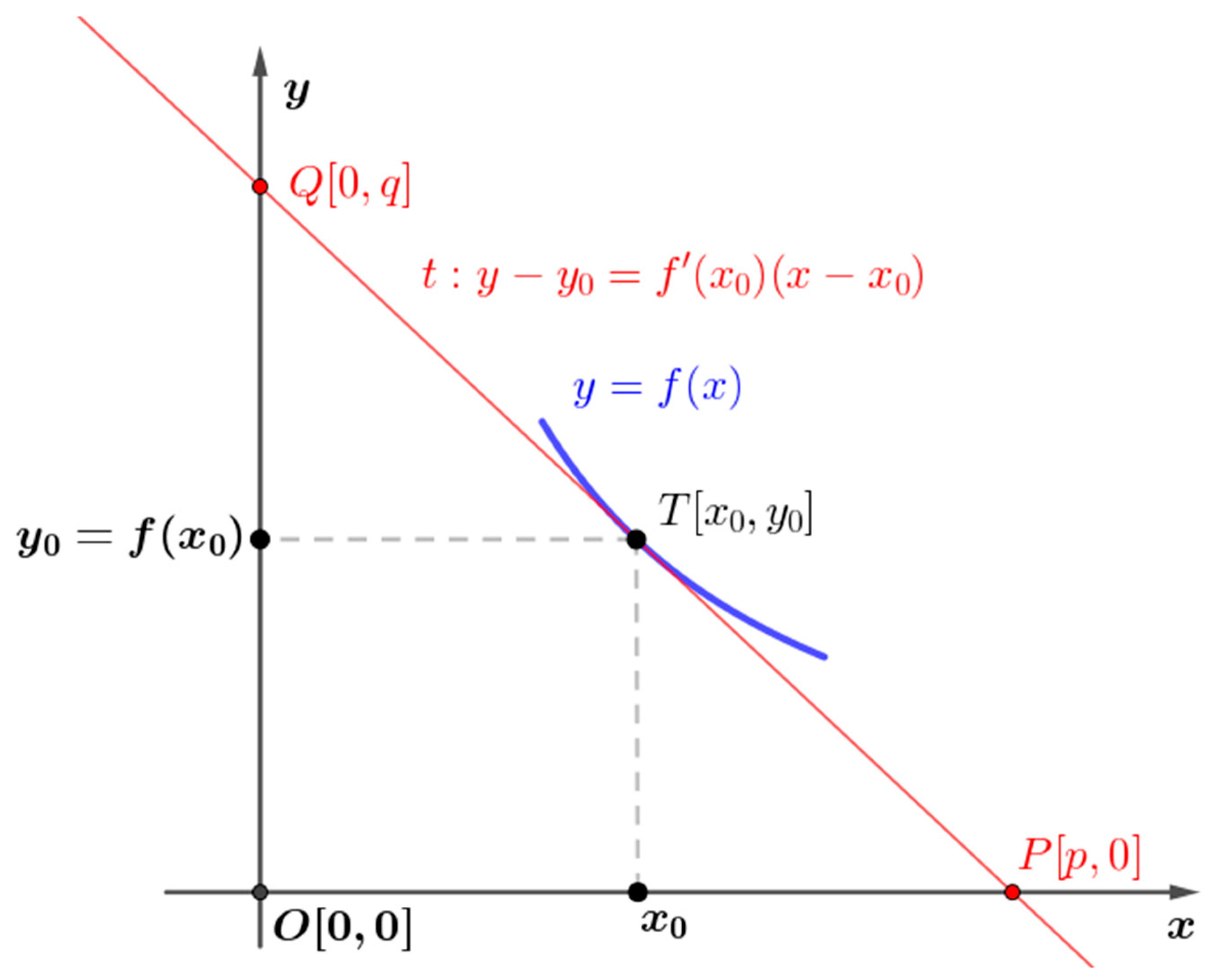
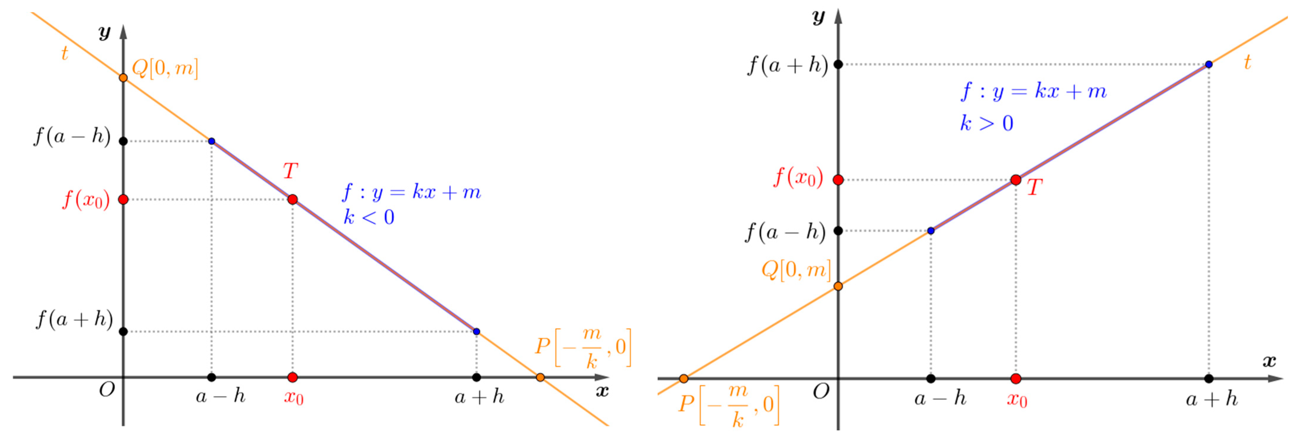
Solution: Consider the graph of the function y = f x defined on the interval J . The tangent line t at the tangent point T x 0 , y 0 , x 0 J , where y 0 = f x 0 , has the following equation:
y y 0 = f x 0 · x x 0 .
The label f x 0 denotes the value of the first derivative y = f x at the point x 0 (see Figure 4).
The point P p , 0 lies on the tangent line t and it holds true that
p = x 0 y 0 f x 0 ,
for f ( x 0 ) 0 .
Similarly, it can be shown that
q = y 0 f x 0 . x 0 = f x 0 . x 0 y 0 f x 0 .
We denote the length P Q of the segment P Q . It holds true that
P Q 2 = p 2 + q 2 = = x 0 y 0 f x 0 2 . 1 + f x 0 2 .
In Equations (16) and (17), we also suppose that f x 0 0 . It follows that the tangent lines with horizontal slopes are excluded.
Let us introduce the following notation:
x 0 = x ,       y 0 = y ,       f x 0 = y ,       G ( x ) = P Q 2
and we follow the function
G x = x y y . 1 + y 2 ,
for y x 0 . We differentiate the function G with respect to the variable x . It holds true that
G x = ± x y y . 1 + y 2     G x = ± y . y y 2 · 1 + y 2 + x y y 1 + y 2     G x = ± y . y + x . y 3 y 2 · 1 + y 2 ,
where y ( x ) 0 ,   1 + y 2 0 for all x J .
Applying the rule for testing extremal values of the differentiable function y = G x and factoring the expression 19 , we obtain
y = 0
y + x . y 3 y 2 · 1 + y 2 = 0 .
Values of x that vanish in Equation (20) and Equation (21), respectively, depend on the prescription of the function y = f x , as well as its domain. We demonstrate this using software, e.g., GeoGebra (v. 5.2.907.0-d).

4. Illustrative Examples: Extremal Lengths for Various Functions f

4.1. Example 1

We begin by considering the linear function f :   y = k x + m ,   k 0   defined on the interval J , e.g., a h ,   a + h for 0 < h R . Applying Equation (20) yields the following results for all x J :
y = k x + m = k   and   y = k x + m = 0 .
Substituting the definition of the linear function y = k x + m into Equation (21) and simplifying the expression yields:
x = m k k 2 + 1 .
Since the graph of the linear function f coincides with the tangent line, we obtain a constant length P Q of the segment P Q given by the following equation:
G x = P Q = m k 1 + k 2 .
This length P Q is constant for fixed values k and m and, crucially, is independent of the point of tangency T , respectively, x 0 a h , a + h (see Figure 5).
If the value m = 0 is trivial, this results in P Q = 0 .

4.2. Example 2

Let f : y = e k x be a function defined on the interval 0 , for k R ,   k > 0 . The following holds true:
y = k . e k x   y = k 2 . e k x
The second derivative of the function f : y = e k x is strictly positive on the interval 0 , . This implies that Equation (20) has no solution.
From Equation (21), we derive the following:
x . k . e k x 3 + e k x k . e k x 2 · 1 + k . e k x 2 = 0 .     e k x . x k 3 . e 2 k x + 1 = 0 .
If we factorize Equation (24), then we obtain e k x = 0 or x k 3 . e 2 k x + 1 = 0 .
The equation e k x = 0 has no solution for x R .

4.2.1. Numerical Approach

Equation (24) indicates a transcendental equation, the solution of which is non-trivial. To estimate the existence of the function’s extremum, we first simulate an approximate numerical solution for Equation (24).
Table 1 presents selected values of x i from the defined domain a , b , 0 < a < b , a , b R . These values are established as a finite arithmetic progression a + i . b a n i = 1 n for i = 0 , 1 , 2 , , n . The range of parameters, as well as the value of parameter k > 0 , can be adjusted as required using a spreadsheet processor (e.g., MS Office Excel or GeoGebra Spreadsheet).
The values in the column for G x i suggest that the function y = G ( x ) is increasing over the given interval a , b and, on first approximation, that it exhibits a nearly linear character (thus without the expected extrema).
Since this involves the calculation of discrete values, only a change in the sign within the values for the column G x i for n = 0 and n = 1 —respectively,   n = 4 and n = 5 —indicates a local extremum at a point x 0 on the subintervals.
By further refining the boundaries of the interval a , b or the step value n , the value of x 0 can be approximated with the desired precision, as shown in Table 2.
We observe sign change in the values in the column for G x i between n = 4 and n = 5 , and for x 0 0.018 , it represents the local maximum G x 0 1.03483 .
As demonstrated in Table 1 and Table 2, successive numerical calculations allow for the estimation of critical points and the approximation of the sought extrema with a predefined level of accuracy.
Using a spreadsheet is an effective method for obtaining output values quickly and efficiently; however, this approach may become cumbersome if the formulae—such as the second derivative of the function y = G x —are highly complex.
On the other hand, detecting potential inflection points through numerical calculations can be problematic (as seen in Table 3 for n = 7 ).
For the reasons outlined above, in this article, a graphical approach is prioritized. The plot of a function—and, more specifically, the plots of its derivatives—provides an immediate overview of the function’s behavior, facilitates the rapid identification of extrema, and enables efficient experimentation with various parameters.
The graphical approach offers the advantage of configurable software settings (e.g., in GeoGebra), allowing for output precision of up to 15 decimal places.

4.2.2. Graphical Approach

Another reason for selecting the software GeoGebra is its functionality, which allows for a comprehensive approach to solving mathematical problems. The software features an Algebra View, a Command Line, a Spreadsheet for data processing, and a Graphics View (two graphics windows). These individual perspectives are dynamically interconnected, meaning that data is shared and updated across all environments simultaneously. Next, we set the values for x 0 to a precision of five decimal places.
We will find an approximate solution of the transcendental equation x k 3 . e 2 k x + 1 = 0 using GeoGebra.
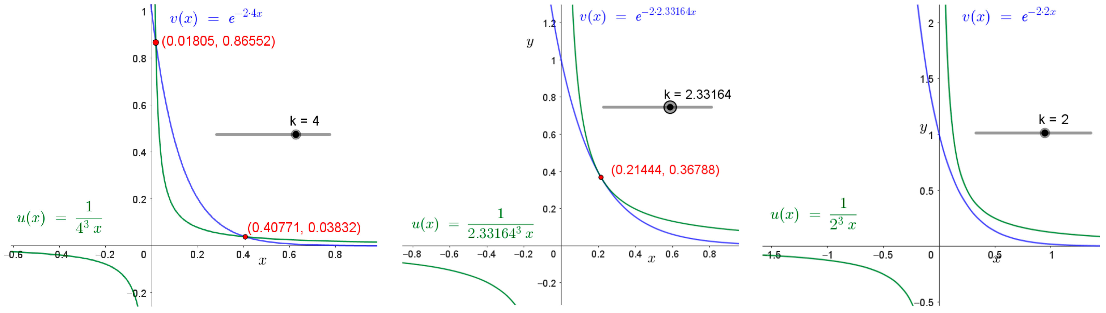
We label u x = 1 k 3 x and v x = e 2 k x and we draw the graphs of these parametric functions in GeoGebra. The existence of intersection points depends on the parameter k (see Figure 6).
To find the solution for x in the transcendental equation
x k 3 . e 2 k x + 1 = 0
we can use a special function known as the Lambert W -function.
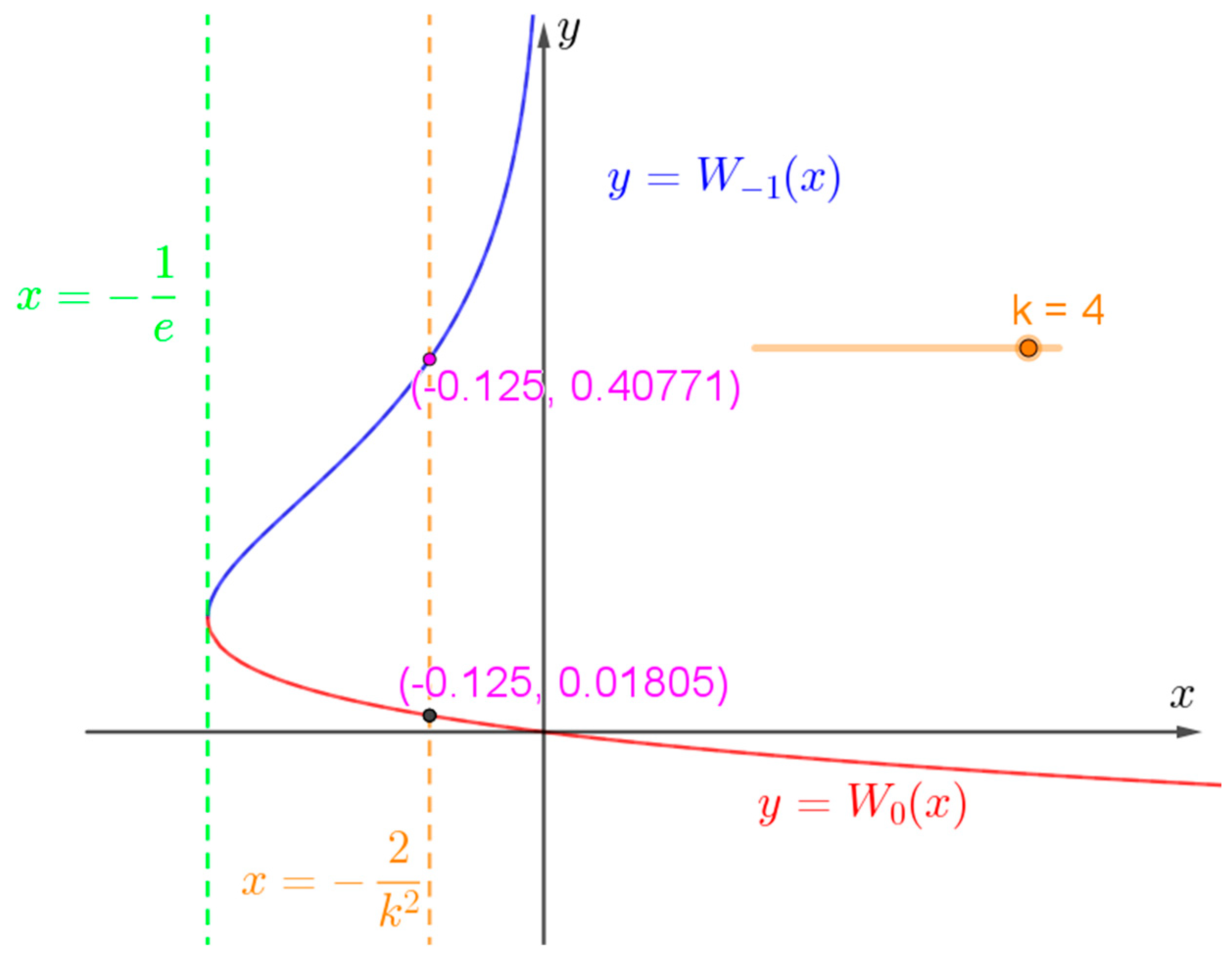
The Lambert W-function is defined in the real domain 1 e ,   , and its graph is divided into two branches W 0 and W 1 [4]. In Figure 7, we use the graph of the Lambert W-function as the inverse function to y = k x e k x .
We adjust the equation in the following form:
2 k x . e 2 k x = 2 k 2 .
It holds true that
x = 1 2 k W 0 , 1 2 k 2 .
The Lambert W -function has a real solution if
2 k 2 1 e
and the number of the real solutions depends on the value of the parameter k :
(a)
Real solutions if 1 e 2 k 2 < 0 ;
(b)
If k is such that k < 2 e 2.33164 , then there are no real solutions.
We evaluate:
(a)
If k = 4 , then x 0 0.01805 and x 1 0.40771 ;
(b)
If k = 2 e , then x 0 , 1 0.21403 .
Substituting y = e k x in Formula (18) yields
G x = x y y . 1 + y 2 = x + 1 k . 1 + k 2 . e 2 k x .
This function is non-negative for x > 0 and k > 0 . This implies that by using Formula (19), we have the second derivative of the function G x in a simpler form:
G x = 1 x k 3 e 2 k x 1 + k 2 e 2 k x     G x = k 4 e 2 k x 2 x k e 2 k x + x k 2 e 2 k x 1 + k 2 e 2 k x 3
Formula (27) will be applied using the second derivative test. If G ( x _ 0   ) < 0 , the function has a local maximum at x 0 . Conversely, if G ( x _ 0   ) > 0 , the function has a local minimum at   x 0 .
In these cases, we have no exact values of the critical points x 1 ,   x 2 —respectively, x 1 , 2 —and the second derivative test only indicates the extrema approximately. We calculate the following:
(a)
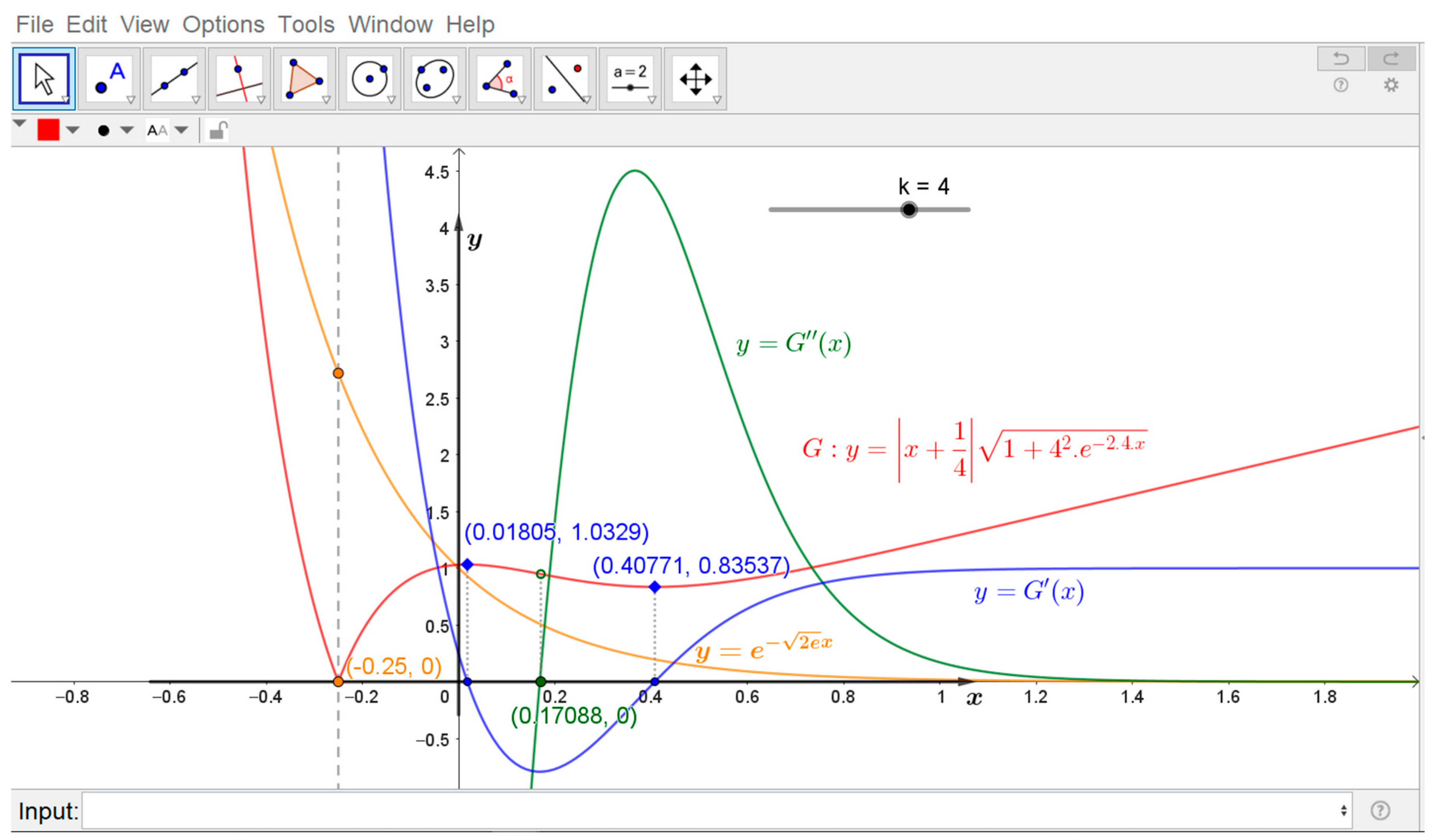
k = 4 is G 0.41 4.37 and G 0.02 12.25 ;
(b)
k = 2 e is G 0.21 0.05 .
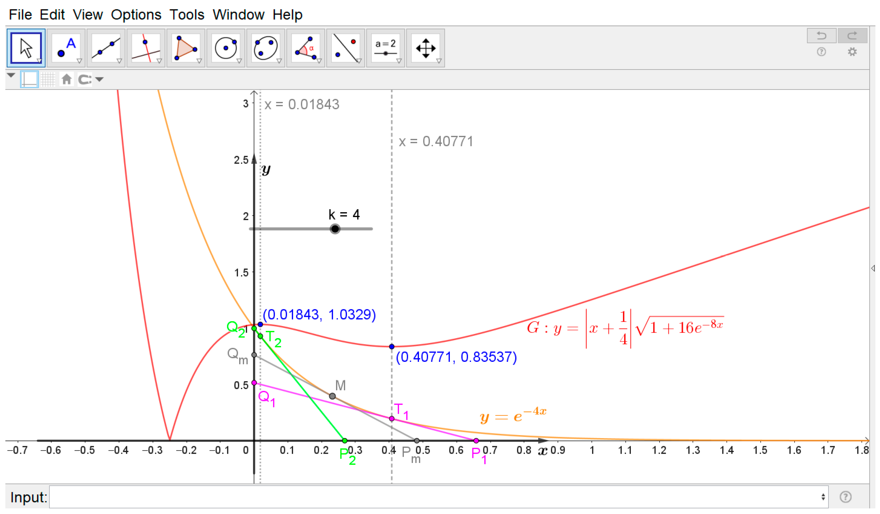
If we use the commands “Derivative(<Function>, <Variable>,<Number>),” the concept can be visualized graphically (see Figure 8).
Using GeoGebra software, we set a slider k = 4 , and we construct the corresponding segments P 1 Q 1 , P 2 Q 2 . These segments lie on the tangent lines to the graph of the given function f : y = e k x at the points x 1 and x 2 . Furthermore, we choose an arbitrary point M x m , f x m on the graph of the function f , and we construct a corresponding segment P m Q m .
By dynamically varying the point M x m , f x m along the graph, we visually compare the corresponding values, which provides visual verification of the extremal solution (see Figure 9).

4.2.3. Brief Analysis of the Graphical Model

Subsequently, we utilized MS Office Excel to perform an analysis of the solution. The percentage value G x i is calculated as
G x i = G x i G r e f G r e f . 100 % ,
where reference value G r e f = G 0.01805 is obtained through the graphical method. The results are presented in Table 4.
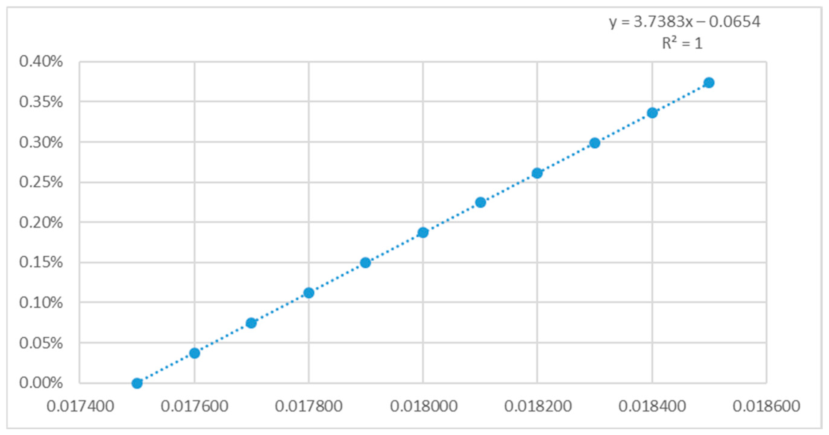
The sensitivity analysis results presented in Table 4 demonstrate a high degree of consistency between the numerical and graphical solutions. The relative deviation initiates at 0.00 % and subsequently exhibits a linear increase with a very low gradient, remaining below the 0.37 % threshold across all observations.
The degree of linearity between x i and G ( x i ) is used to assess the stability of the numerical solution within the given interval. The regression line is of the form G x = a 1 x + a 2 .
The regression equation y = 3.7383 x 0.0654 , characterized by correlation coefficient r = 1.00 and coefficient of determination R 2 = 1.00 , demonstrates a functional identity between the numerical datasets.
The residual standard deviation s r e z = 0 . This means that the model is suitable for predicting G x values at specified values of x , and the proposed spreadsheet model perfectly replicates the graphical reference system without any statistical variance (see Figure 10).
An analogous situation for x 0.406 ,   0.408 , n = 10 and k = 4 , is observed for the extremum at the point x 0 = 0.40771 , where the reference value is G r e f = G x 0 = 0.83537 . The equation of the regression line is y = 1.5244 x 0.6189 , characterized by correlation coefficient r = 1.00 and coefficient of determination R 2 = 1.00 .
If we set x ( 0.214 ;   0.215 ), n = 10 for k = 2 e , and use the reference value G r e f x 0 = 1.114270 , then we can calculate the equation of regression line in the form of   y = 1.5555 x 0.3329 (also with r = 1.00 and R 2 = 1.00 ) .
A high correlation indicates a strong agreement between the datasets. This can be verified experimentally by setting the calculations in both MS Excel and GeoGebra to 10 decimal places.
Using the commands Sequence(<Expression>, <Variable>, <Start Value>, <End Value>), we calculate the sequences of values for x i , i = 1, 2,…, n, f ( x i ) ,   f ( x i ) and G ( x i ) , which are then transferred to the Spreadsheet using the FillColumn(<Column>, <List>) command. We leave it to the reader to verify that the datasets match in every single output.
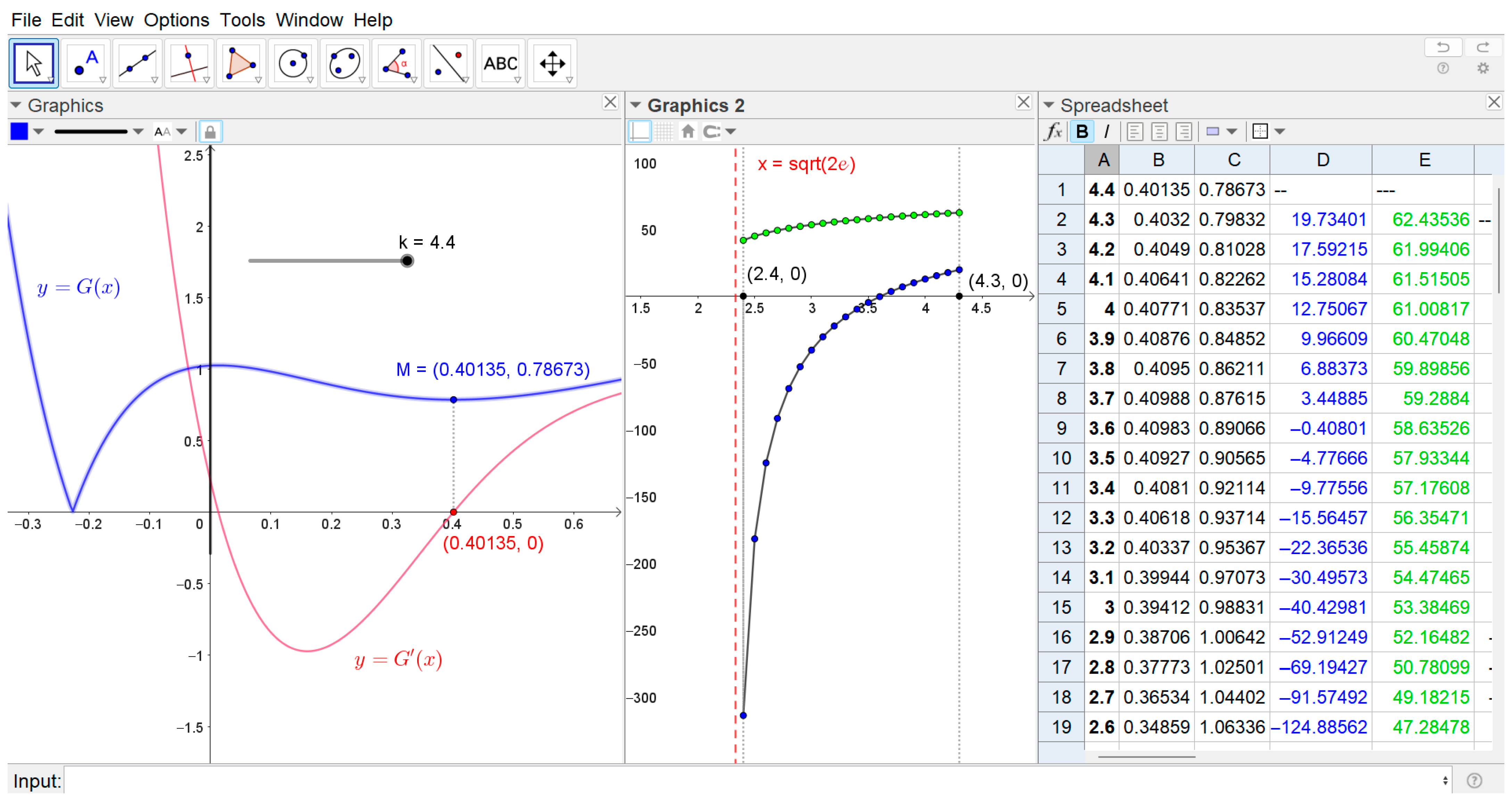
Using GeoGebra, we perform a sensitivity analysis on the parameter k in the critical points.
Consider Equation (18) with the function y = e k x . Using a slider, we set k 2.4 , , 4.3 , 4.4 with a step increment of 0.1 . We conduct a sensitivity analysis of the critical point that represents the local minimum of the function y = G ( x ) .
On the graph of y = G ( x ) , we construct a point M x 0 ,   G x 0 . The point x 0 is a critical point at which the graph of the function y = G x actually intersects the x -axis.
We import the coordinate data of point M into the Spreadsheet environment using commands, while the value of the slider k changes from k down to 2.4 .
We define the sensitivity index S x as follows:
S x = x x k k . 100 % = x i x i 1 x i 1 0.1 k i . 100 % ,
for k = 4.4 ,   4.3 . ,   ,   2.4 .
By analogy, we define the sensitivity index S y as follows:
S y = y y k k . 100 %
and after defining the input parameters, the output values are calculated by Geogebra Classic 5.2.907.0-d.
The sensitivity indices are classified according to a three-level sensitivity scale: low (below 10%); moderate (10–20%); and high (above 20%) [5].
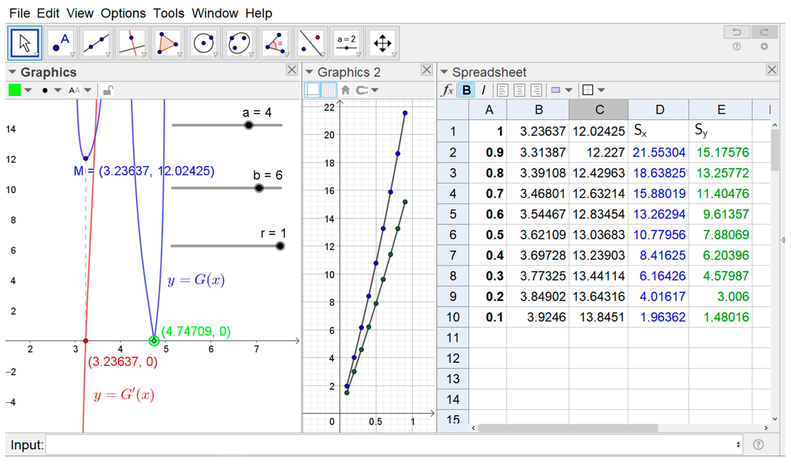
The sensitivity index S x exhibits a decreasing trend across the observations, and it holds true that the mean   S x ¯ 20.93 % (after excluding the outliers x 181.73475 and x 313.69379 ), the median S x ~ −7.28%, and the standard deviation S D x   40.84 % if the range is from 124.89 % to 19.73 % .
These characteristics indicate a high-to-extreme level of sensitivity, dominated by strong negative responses and substantial variability.
As the value of k 2 e (the condition for the existence of an extremum), the model becomes highly sensitive, and the value of   k significantly impacts the critical point x 0 .
Regarding the sensitivity index S y , the model exhibits low sensitivity to change, ranging from 62.44 % to 41.74 % , with a mean S y ¯   55.30 % , median S y ~ 56.77%, and a standard deviation S D y 5.84 % .
These characteristics indicate a high but stable level of sensitivity, with an average change of 1.05% between two consecutive values.
The data were processed using GeoGebra commands Mean(<LISTofRawData>), Median(<LISTofRawData>), SD(<LISTofRawData>) and finally graphically illustrated in the Graphics 2 view (see Figure 11).
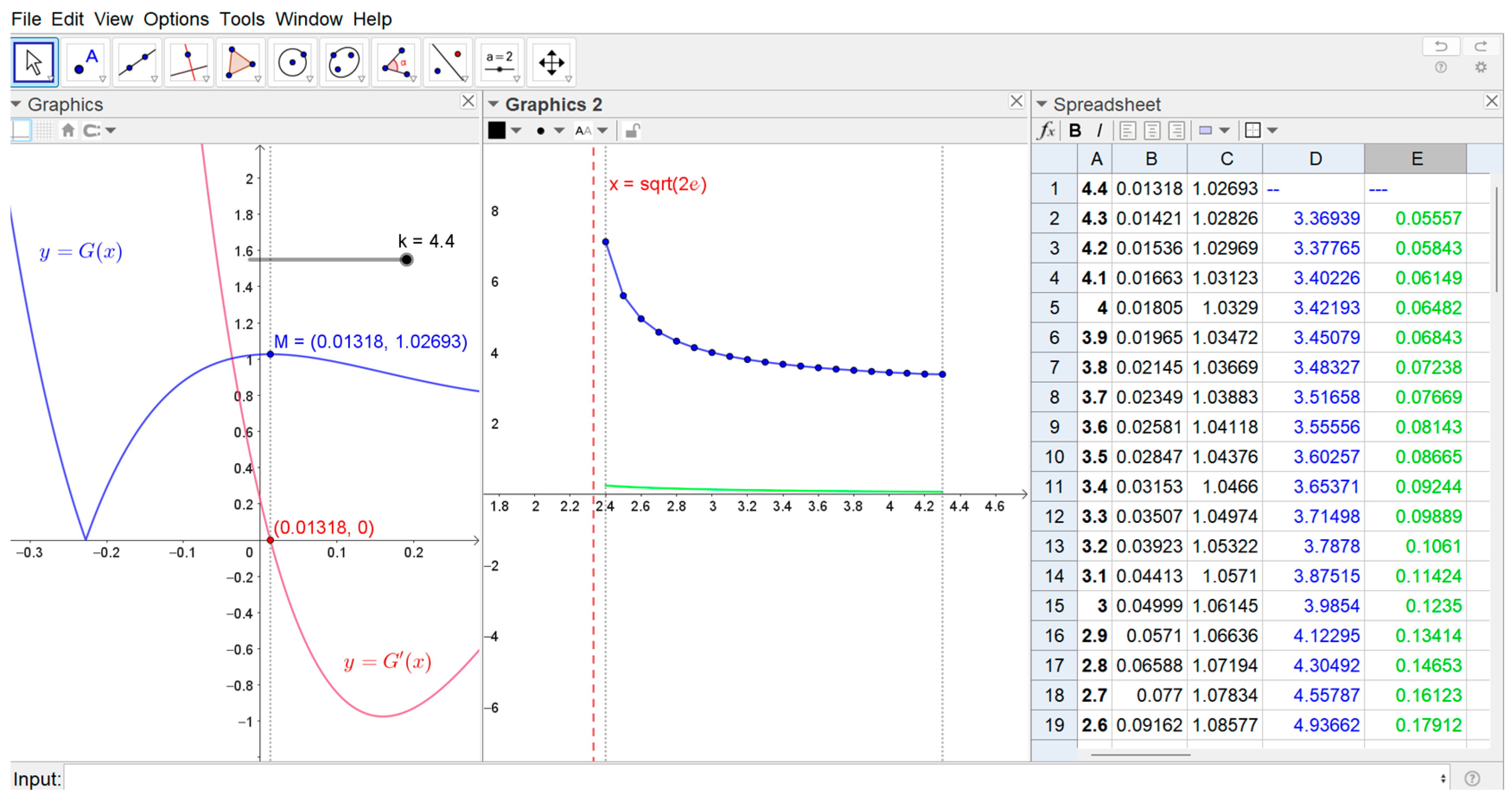
One can perform a similar analysis for the critical point x 0 correspondig to the local maximum of the given function y = G x (see Figure 12).
Remark 3.
Due to the significant difference in index values and in the interest of comparing the sensitivity of both indices, we do not display the corresponding indices as percentages in the Graphics 2 window.
The analysis of the sensitivity index S x indicates a high level of sensitivity, with the mean   S x ¯  ≈ 394.10% and the median S x ~ 368.41%. The standard deviation S D _ x 93.82 % for the range is from 337.76 % to 710.73 % , which indicates a high-to-extreme level of sensitivity, with an average change of 20.75% between two consecutive values.
As the value of k 2 e (the condition for the existence of an extremum), the model becomes highly sensitive, and the value k significantly impacts the value of the critical point x 0 .
As for the sensitivity index S y , in a range from 5.55% to 23.34%, we observe the mean S y ¯ 10.83 % and the median S y ~ 9.57%. S D y 4.77 % and there is an average change of 1.05% between two consecutive values.
The values indicate moderate model sensitivity, and small changes in the input lead to relatively small but still significant changes in the output.
The standard deviation indicates that individual values differ only slightly from the mean, meaning that the model responds relatively consistently to different inputs with y values. This is not an extremely sensitive system; rather, it is a stable one with moderate variations (see Figure 12, window Graphics 2).

4.2.4. Visualization of the Solution Related to the Function y = e k x

By extending the domain to interval , and constructing the tangent line at point M 0 [ 1 k ,   e ] , we find that this tangent line passes through the origin O [ 0 , 0 ] . The corresponding segment P m Q m has the length P m Q m = 0 , which represents the global minimum of the function f : y = e k x .
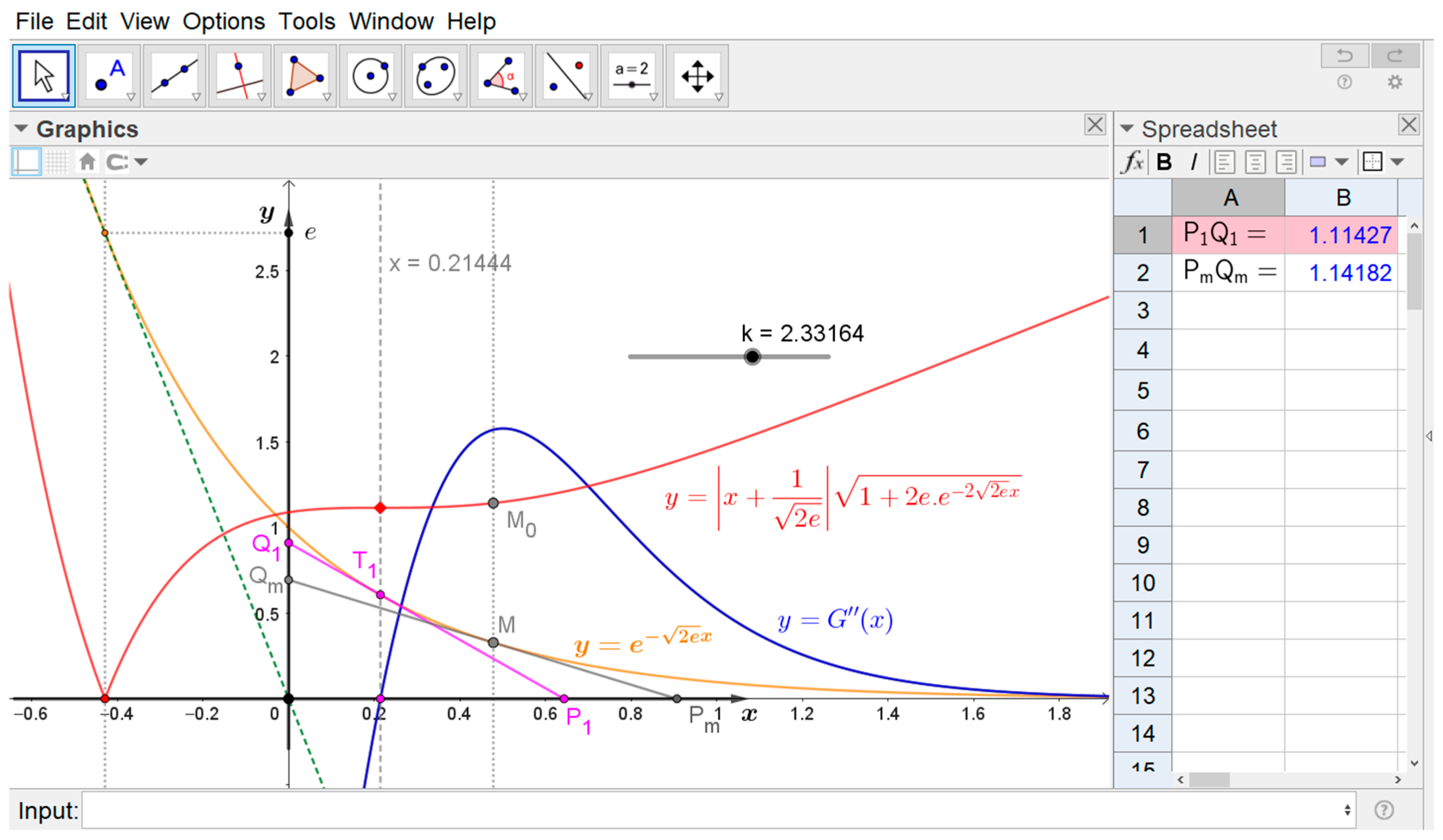
If we set k = 2 e 2.33164 , then the value G 0.21444 0.06 indicates the inflection point (see Figure 13).
Graphically, the second derivative y = G x is computed using the Derivative(<Function>, <Number>) command in GeoGebra.
The graph of the second derivative y = G x intersects the x axis at x 0.21444 . The sign of the second derivative changes from negative (left neighborhood of x 0.21444 ) to positive (right neighborhood). Consequently, the function has an inflection point at x 0.21444 .

4.3. Example 3

Consider the function f : y = b r 2 x a 2 defined on the interval J = a r , a , where 0 < r a b , a , b , r R . Its graph is a quarter circle with a center M a , b and a radius r .
It holds true that
y = b r 2 x a 2 = = x a r 2 x a 2 ,
y = x a r 2 x a 2 = = r 2 r 2 x a 2 3 2 .
Evidently, by applying the function f to Equation (20) there is no solution.
Substituting the quadratic function into Equation (21) and simplifying leads to an irrational equation:
x x a r 2 x a 2 3 + b r 2 x a 2 = 0     x 4 3 a x 3 + 3 a 2 x 2 a 3 x r 2 x a 2 3 + b r 2 x a 2 = 0
This partial result yields an equation of the 8 -th degree. Since its solution is non-trivial in the general case, we will again use the graphical method to find an approximate solution.
First, we define parameters a , b , r . In the input bar, we define the function
f :   y = b r 2 x a 2
using the Geogebra commands Function(<Function>, <Start x-Value>, <End x-Value>) and Derivative(<Function>). We directly calculate the derivative which corresponds to Formula (21).

4.3.1. Brief Sensitivity Analysis of the Graphical Model

Using GeoGebra, we also perform a sensitivity analysis on the parameter r .
Consider the function f :   y = b r 2 x a 2   with domain x a r , a + r and substitute the function into Formula (18). Using the sliders, we set the parameters a = 4 ,   b = 6 , and r 0 , 1 , with a step increment of 0.1 .
We construct the point M x 0 ,   G x 0 , where x 0 is the point at which the graph of the function y = G x intersects the x -axis. We import the coordinate data of point M into Spreadsheet using the commands (Record to Spreadsheet), while the value of the slider r changes from 1 to 0.1 .
We apply the sensitivity indices S x and S y , which are calculated in Spreadsheet, and corresponding lists of points are displayed in Graphics 2, as shown in Figure 15.
Using Geogebra commands for the sensitivity index S x   we calculate the mean S x ¯ = 11.18603 % , the median S x ~ = −7.27614%, and the standard deviation S D x = 6.31466 . The range of the dataset is from 1.96362 to 21.55304 .
The sensitivity index S x suggests a moderate level of sensitivity. Standard deviation reflects a considerate degree of variability around the mean. The average change between two consecutive observations amounting to 2.45% indicates that fluctuations in the sensitivity index S x are moderate.
A similar situation is observed for the sensitivity index S y with range from 1.48016 to 15.17576 ; the mean   S y ¯ = 8.06694%, S y ~ = 7.88069 , and S D y = 4.4181 .
In Figure 14, one can see in the Graphics 2 window that the model exhibits low sensitivity to change for fixed a = 4 ,   b = 6 , and r 0 . The simulation also suggests that for r 0 , we are approaching the solution to the original problem, which is given by Equation (13).

4.3.2. Visualization of the Solution Related to the Function y = b r 2 x a 2

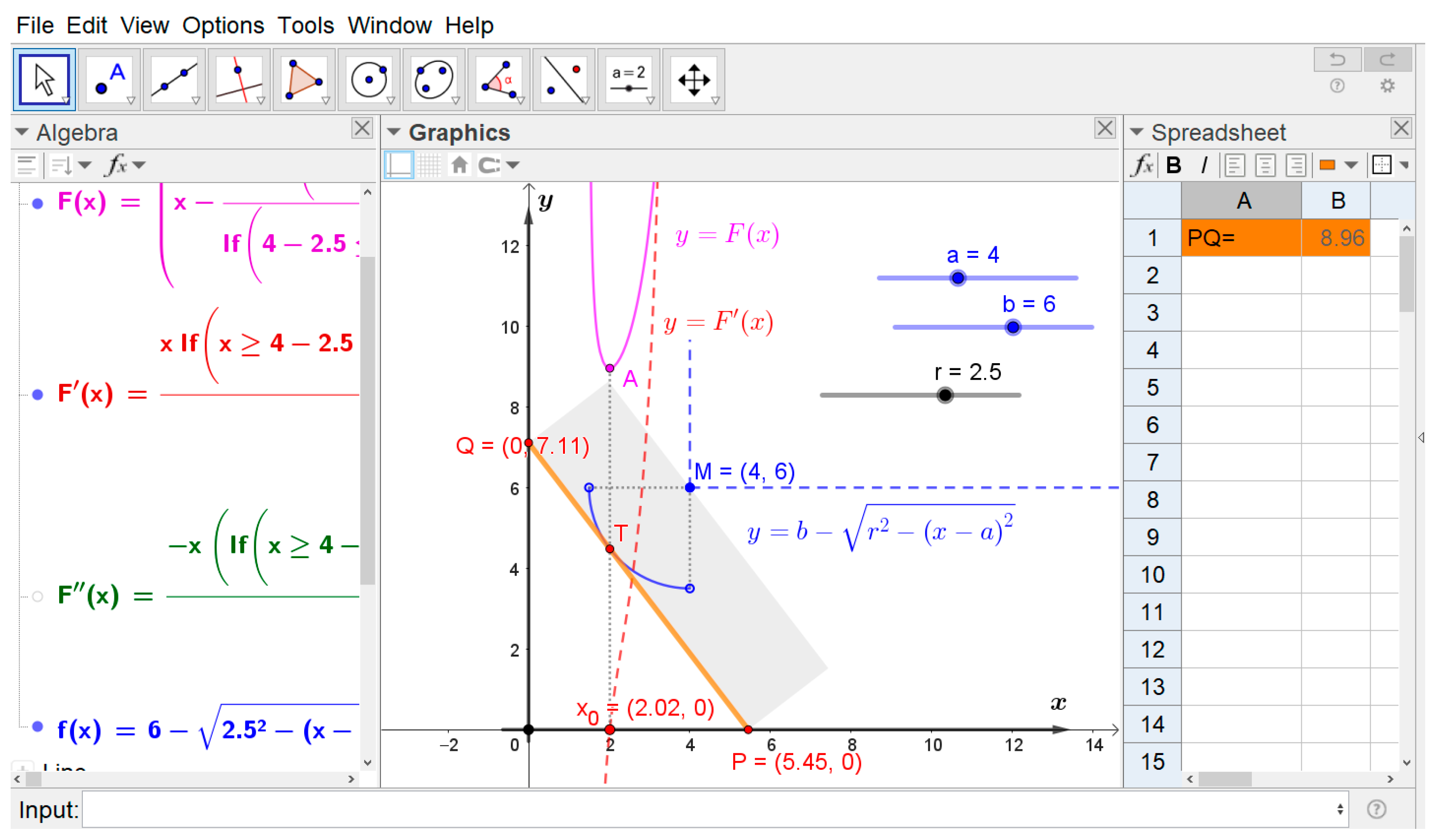
Finally, we would like to point out that the solution addresses the problem of extreme length for the log, which is modeled as a rectangle of width r .
We set the parameters a = 4 ,   b = 6 , and r = 2.5 . The critical point is   x 0 2.02 , where the point x 0 is found by intersecting the graph of its derivative y = G ( x ) and the x -axis. We obtain the tangency point T x 0 , y 0 , where y 0 = f x 0 4.48 .
The tangent line at point T x 0 , y 0 approximately intersects the axes at points P 5.45 , 0 and Q 0 , 7.11 , and we calculate P Q 8.96 . This value is the minimum of the function y = G x (see Figure 15).
Remark 4.
In 1966, mathematician Leo Moser formulated a problem that is now known as the Moving Sofa Problem. The essence of the problem is finding the largest area planar shape (sofa) that can move around a right-angled corner in a hallway of unit width [6].

5. Problem of Constant Length of the Segment P Q

In the previous examples, we have shown that the length of the line segment P Q depends on the function y = f ( x ) and its domain. Let us investigate the problem of whether there exists such a function y = f ( x ) for which it holds that
P Q = k , k > 0 , k R .
Formula (18) implies that
x y y . 1 + y 2 = k     y = x . y k . y 1 + y 2 .
Equation (31) is Clairaut’s differential equation [7] in the general form:
y = x . y + g y ,
where g is a function of variable y . The general solution of Equation (31) is
y = x . c     k . c 1 + c 2 ,
where c R is the parameter.
Geometrically, the solution is a system of two parallel lines. This result corresponds to the solution to Example 1.
The envelope of the system of integral curves (solutions) is defined as a curve that is tangential to every solution of the given differential equation at at least one point. The envelope itself constitutes a solution, specifically a singular solution (at which the uniqueness of the solution to the Cauchy problem is violated).
The equation of the envelope is derived from a system of two equations, which consists of the solution itself and its derivative with respect to parameter c .
Thus, we obtain a system of equations:
y = x . c     k . c 1 + c 2   d y d c = 0 = x k . 1 + c 2 k . c . 2 c 2 1 + c 2 1 + c 2 = = x k 1 + c 2 3 2
For illustrative purposes, consider the following system (the same result can be derived using the second system of the equations as well):
x = + k 1 + c 2 3 2 y = x . c     k . c 1 + c 2
We substitute the variable x and simplify
y = k 1 + c 2 . 1 + c 2 . c k . c 1 + c 2 = = k . c 3 1 + c 2 3 2
Parameter c is eliminated from the equations as follows:
x k 2 3 = 1 1 + c 2   y k 2 3 = c 2 1 + c 2 = 1 + c 2 1 1 + c 2 = 1 1 1 + c 2 = 1 x k 2 3
The result is the equation of the astroid [8] in implicit form:
x 2 3 + y 2 3 = k 2 3 .
This is consistent with the solution to the original problem concerning the maximum length of a log that can be floated through two mutually perpendicular navigable canals.
Finally, we proceed to model the situation in GeoGebra.
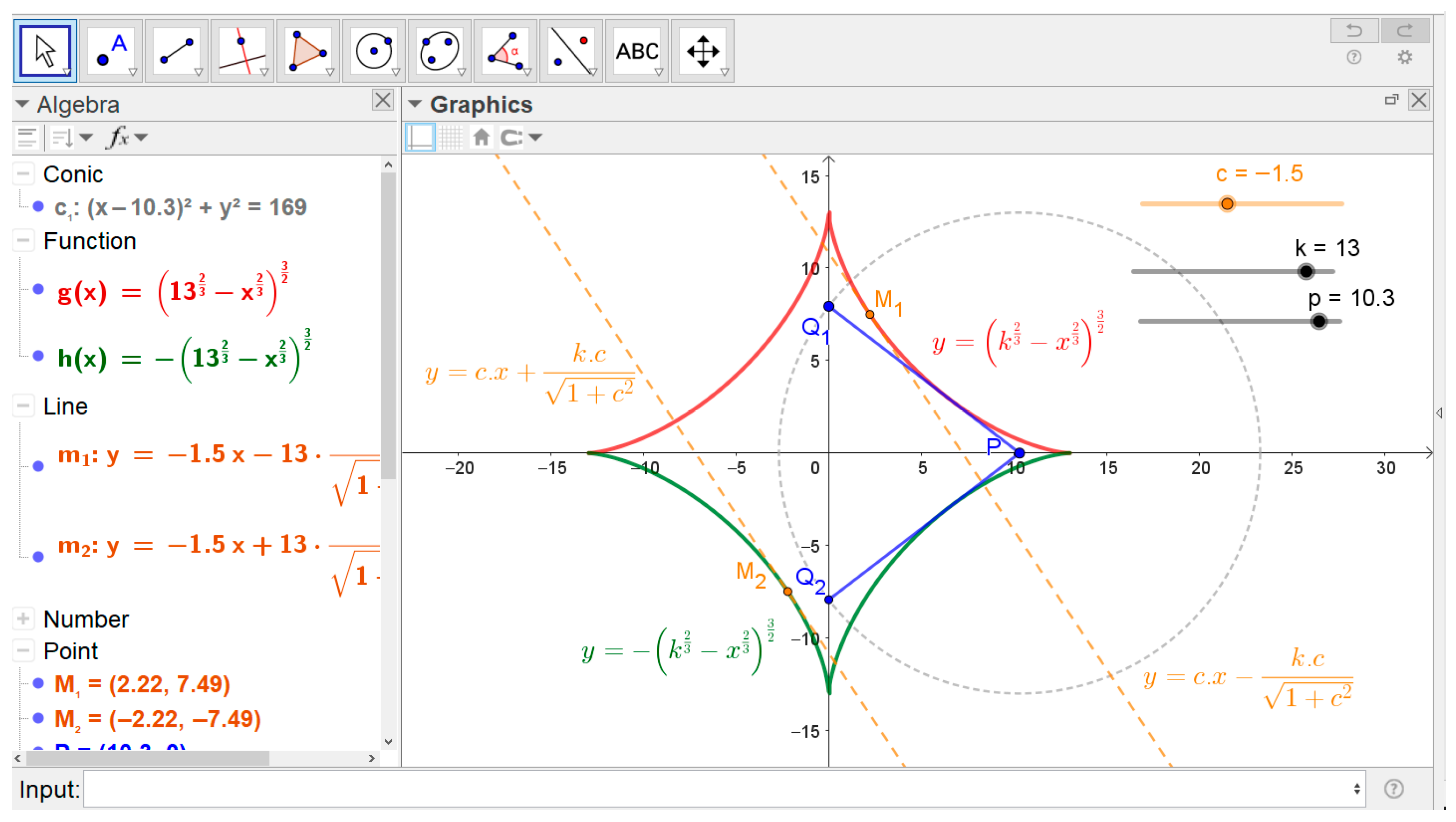
We set the parameters k R ,   k > 0 ,   c R and p k , k . An auxiliary circle with the center P p , 0 and the radius k intersects the y -axis at points Q 1 0 , q and Q 2 [ 0 ,   q ] . We draw the line-segments P Q 1 and P Q 2 .
Subsequently, we insert the functions
y = ± k 2 / 3 x 2 / 3 3 2
into the input bar.
We observe that by changing the position of the point P , we model the tangents, P Q 1 and P Q 2 , that generate the envelope in the shape of the asteroid (see Figure 16). The points
M 1 k 1 + c 2 3 2 , k . c 3 1 + c 2 3 2 ,   M 2 k 1 + c 2 3 2 , k . c 3 1 + c 2 3 2
are the points of tangency for the tangent lines defined by Equation (32).
6. Discussion

Mathematical modeling is a key component of mathematical applications and education. It enables us to comprehend the intricate mechanisms of the real world. While it is impossible to capture every facet of a real situation using a model, reducing complexity makes models usable.
Models always have a simulative and an exploratory function. However, excessive focus on interesting questions within the model or generalizing the nature of the original situation can lead to computational complications and more challenging tasks [9].
At the same time, this focus can motivate the further advancement of knowledge and generalization, which can take various forms. For example, we can apply procedures that have already been used after changing the input conditions, model the problem in higher dimensions, use other (curvilinear) coordinate systems to facilitate calculations or solve the original problem in other geometries.
It is useful if the model is visual. In this article, we present a model for solving an optimization problem based on a specific application task: finding the longest wooden log that can ideally be transported through two perpendicular water canals. As mentioned above, we opted for a graphical solution method for reasons of visualization, as this is a natural and important element of mathematical thinking and is key to discovering relationships and connections between mathematical objects [10].
The problem is generalized by changing the input conditions, leading to the application of calculus and the solving of algebraic equations. These generalizations encourage the use of the dynamic geometric software GeoGebra, which is available as freeware, due to the possibility of sharing common data between graphic and analytical inputs without having to transfer them to other software, applications, or spreadsheets for calculations.
In advanced mathematics, students often struggle to connect algebraic derivative tests with geometric reality. We believe that the graphical method serves as a cognitive bridge, allowing students to use GeoGebra as a “digital laboratory” where they can verify analytical proofs through rigorous geometric construction. This encourages a deeper conceptual understanding of the relationship between a function’s local behavior and its derivative.
This method is ideally suited for inquiry-based learning environments. Teachers can present a complex geometric problem where the solution is not immediately obvious, and students can use the proposed GeoGebra workflow to form hypotheses, test them through precise construction, and subsequently confirm their validity using analytical derivation.
In geometry curricula, this method can be integrated into modules focusing on spatial modeling. By manipulating parameters in real-time and observing the immediate effect on extrema and tangents, students can develop a dynamic geometric intuition that static textbook examples cannot provide.
In terms of its content, this is an interesting topic that connects multiple mathematical disciplines and demonstrates the practical application of mathematics. This makes the topic accessible to undergraduates, and this article could be used as an inspiring teaching resource; e.g., the simulation in Figure 15 could be used to introduce the well-known “Moving Sofa Problem,” first formulated in 1966, but still classified as an open problem. By exploring these mathematical challenges through analytical and visual methods, students can develop a more intuitive understanding of complex phenomena. Ultimately, this approach should inspire a deeper interest in the continuous evolution of mathematical discovery.

Funding

The APC was funded by the Faculty of Natural Sciences and Informatics, Constantine the Philosopher University in Nitra.

Data Availability Statement

The original contributions presented in this study are included in the article. Further inquiries can be directed to the corresponding author.

Acknowledgments

The author is grateful to the reviewers for their valuable suggestions.

Conflicts of Interest

The author declares no conflicts of interest.

References

  1. Tihomirov, V.M. Extremal problems-past and present. Teach. Math. 2002, 2, 59–69. [Google Scholar]
  2. Fulier, J. Prvky konštruktivizmu pri riešení extremálnych úloh. In Zborník Príspevkov zo Seminára Konštruktivizmus vo Vyučovaní Matematiky a Budovanie Geometrických Predstáv; Šedivý, O., Ed.; FPV UKF: Nitre, Slovakia, 2010; pp. 67–77. [Google Scholar]
  3. Eliáš, J.; Horváth, J.; Kajan, J. Zbierka Úloh z Vyššej Matematiky II; Alfa: Bratislava, Slovakia, 1966; p. 113. [Google Scholar]
  4. Weisstein, E.W. Lambert W-Function. MathWorld—A Wolfram Resource. Available online: https://mathworld.wolfram.com/LambertW-Function.html (accessed on 20 November 2025).
  5. Borgonovo, E.; Plischke, E. Sensitive analysis: A review of recent advances. Eur. J. Oper. Res. 2016, 248, 869–887. [Google Scholar] [CrossRef]
  6. Weisstein, E.W. “Moving Sofa Problem.” From MathWorld—A Wolfram Resource. Available online: https://mathworld.wolfram.com/MovingSofaProblem.html (accessed on 9 January 2026).
  7. Weisstein, E.W. Clairaut’s Differential Equation. From MathWorld—A Wolfram Resource. Available online: https://mathworld.wolfram.com/ClairautsDifferentialEquation.html (accessed on 20 November 2025).
  8. Weisstein, E.W. Astroid. From MathWorld—A Wolfram Resource. Available online: https://mathworld.wolfram.com/Astroid.html (accessed on 20 November 2025).
  9. Fischer, R.; Malle, G. Mensch und Mathematik; Profil: Munich, Germany, 2004. [Google Scholar]
  10. Fulier, J. Some Remarks on Aspects of Visualization in Mathematical Education. Acta Math. Niriensia 2018, 4, 24–38. [Google Scholar] [CrossRef]
Figure 1. Situational diagram of the original problem.
Mathematics 14 00386 g001
Figure 2. Geometric representation of the problem.
Mathematics 14 00386 g002
Figure 3. Graphical solution of the original problem for a = 4 m   a n d   b = 6 m .
Mathematics 14 00386 g003
Figure 4. General position of the tangent line t and its point T of tangency.
Mathematics 14 00386 g004
Figure 5. Illustration of the constant segment length P Q for the linear function y = f ( x ) .
Mathematics 14 00386 g005
Figure 6. Intersection points of the graphs of the functions u x , v x for k = 4 , 2 e , 2 .
Mathematics 14 00386 g006
Figure 7. Graphical solution using the Lambert W-function.
Mathematics 14 00386 g007
Figure 8. Visualization of the local extrema of the function y = G ( x ) and its derivatives for k = 4 .
Mathematics 14 00386 g008
Figure 9. Visualization of the local extrema for k = 4 .
Mathematics 14 00386 g009
Figure 10. Linear regression with the line G ( x ) = 3.7383 x 0.0654 for x 0 0.01805 and k = 4 .
Mathematics 14 00386 g010
Figure 11. Sensitivity analysis of the model for the local minimum in GeoGebra.
Mathematics 14 00386 g011
Figure 12. Sensitivity analysis of the model for the local maximum in GeoGebra.
Mathematics 14 00386 g012
Figure 13. Visualization of the inflection point of the function y = G ( x ) at x 0 0.21444 for k = 2 e .
Mathematics 14 00386 g013
Figure 14. Sensitivity analysis of the model for the local extremum in GeoGebra.
Mathematics 14 00386 g014
Figure 15. Graphical solution of Example 3 for a = 4 ,   b = 6 , and   r = 2.5 in GeoGebra.
Mathematics 14 00386 g015
Figure 16. Visualization of the solution through the astroid in GeoGebra.
Mathematics 14 00386 g016
Table 1. Numerical estimation of extrema for the function y = G ( x ) for k = 4 on interval 0.01 ,   1.00 .
n x i f ( x i ) f ( x i ) f ( x i ) G ( x i ) G ( x i )
0 0.010000 0.9608 3.8432 15.3726 1.032493 0.103045152
1 0.109000 0.6466 2.5865 10.3459 1.425635 0.69121129
2 0.208000 0.4352 1.7407 6.9628 1.818777 0.757669487
3 0.307000 0.2929 1.1715 4.6860 2.211919 0.444956373
4 0.406000 0.1971 0.7884 3.1537 2.605060 0.007480611
5 0.505000 0.1327 0.5306 2.1225 2.998202 0.380942476
6 0.604000 0.0893 0.3571 1.4284 3.391344 0.651588044
7 0.703000 0.0601 0.2403 0.9614 3.784485 0.814380908
8 0.802000 0.0404 0.1617 0.6470 4.177627 0.904315878
9 0.901000 0.0272 0.1089 0.4354 4.570769 0.951669783
10 1.000000 0.0183 0.0733 0.2931 4.963911 0.975914833
Table 2. Numerical estimation of extrema for the function y = G ( x ) for k = 4 on interval 0.0175 ,   0.0185 .
n x i f ( x i ) f ( x i ) f ( x i ) G ( x i ) G ( x i )
0 0.01750.9324−3.729614.91831.0329010.006816019
1 0.01760.9320−3.728114.91231.0332870.00557997
2 0.01770.9316−3.726614.90641.0336730.00434514
3 0.01780.9313−3.725114.90041.0340590.003111529
4 0.01790.9309−3.723614.89451.0344460.001879136
5 0.01800.9305−3.722114.88851.0348320.00064796
6 0.01810.9302−3.720614.88251.035218−0.000581999
7 0.01820.9298−3.719114.87661.035604−0.001810742
8 0.01830.9294−3.717714.87061.035990−0.003038269
9 0.01840.9290−3.716214.86471.036376−0.004264582
10 0.01850.9287−3.714714.85871.036762−0.005489682
Table 3. Numerical estimation of extrema for the function y = G x   for k = 2 e on interval 0.20 ,   0.22 .
n x i f ( x i ) f ( x i ) f ( x i ) G ( x i ) G ( x i )
0 0.20000.6273−1.46263.41041.1142620.0013386943
1 0.20200.6244−1.45583.39451.1178050.0009905146
2 0.20400.6215−1.44913.37871.1213490.0006954978
3 0.20600.6186−1.44233.36301.1248920.0004531672
4 0.20800.6157−1.43563.34731.1284360.0002630473
5 0.21000.6128−1.42893.33181.1319800.0001246644
6 0.21200.6100−1.42233.31631.1355230.0000375462
7 0.21400.6072−1.41573.30081.1390670.0000012216
8 0.21600.6043−1.40913.28551.1426110.0000152212
9 0.21800.6015−1.40253.27021.1461540.0000790771
10 0.22000.5987−1.39603.25501.1496980.0001923228
Table 4. Analysis of the extremum for the function y = G ( x 0 ) for k = 4 on interval 0.0175 ,   0.0185 .
n 012345678910
x i   0.017500.017600.017700.017800.017900.018000.018100.018200.018300.018400.01850
f ( x i ) 0.93240.93200.93160.93130.93090.93050.93020.92980.92940.92900.9287
G ( x i ) 1.032901.033291.033671.034061.034451.034831.035221.035601.035991.036381.03676
G ( x i ) 0.00%0.04%0.07%0.11%0.15%0.19%0.22%0.26%0.30%0.34%0.37%
Disclaimer/Publisher’s Note: The statements, opinions and data contained in all publications are solely those of the individual author(s) and contributor(s) and not of MDPI and/or the editor(s). MDPI and/or the editor(s) disclaim responsibility for any injury to people or property resulting from any ideas, methods, instructions or products referred to in the content.