Is Weniger’s Transformation Capable of Simulating the Stieltjes Function Branch Cut?

Abstract

The resummation of Stieltjes series remains a key challenge in mathematical physics, especially when Padé approximants fail, as in the case of superfactorially divergent series. Weniger’s $\delta$-transformation, which incorporates a priori structural information on Stieltjes series, offers a superior framework with respect to Padé. In the present work, the following fundamental question is addressed: Is the $\delta$-transformation, once it is applied to a typical Stieltjes series, capable of correctly simulating the branch cut structure of the corresponding Stieltjes function? Here, it is proved that the intrinsic log-convexity of the Stieltjes moment sequence (guaranteed via the positivity of Hankel’s determinants) allows the necessary condition for $\delta$ to have all real poles to be satisfied. The same condition, however, is not sufficient to guarantee this. In attempting to bridge such a gap, we propose a mechanism rooted in the iterative action of a specific linear differential operator acting on a class of suitable auxiliary log-concave polynomials. To this end, we show that the denominator of the $\delta$-approximants can always be recast as a high-order derivative of a log-concave polynomial. Then, on invoking the Gauss–Lucas theorem, a consistent geometrical justification of the $\delta$ pole positioning is proposed. Through such an approach, the pole alignment along the negative real axis can be viewed as the result of the progressive restriction of the convex hull under differentiation. Since a fully rigorous proof of this conjecture remains an open challenge, in order to substantiate it, a comprehensive numerical investigation across an extensive catalog of Stieltjes series is proposed. Our results provide systematic evidence of the potential $\delta$-transformation ability to mimic the singularity structure of several target functions, including those involving superfactorial divergences.

1. Introduction

The resummation of Stieltjes series remains a pivotal challenge in mathematical physics, from strongly divergent expansions [1,2,3] to centenary problems in Celestial Mechanics [4,5]. Customarily, this task is entrusted to Padé approximants, implemented via Wynn’s epsilon algorithm [6]. While a robust convergence theory exists for Padé approximants to Stieltjes series (see, for instance, Baker and Graves-Morris [7]), this supremacy is not absolute. In some important cases, such as the octic anharmonic oscillator [8,9,10], Padé-based methods fail to retrieve the correct energy spectrum. These limitations of Padé approximants also stem from their inability to incorporate important a priori structural information regarding the character of the Stieltjes series. For example, Stieltjes functions truncation errors are governed by converging factors that must satisfy a linear first-order difference equation [11]. Since such equations are naturally solved by inverse factorial series, any resummation tool capable of integrating this structural feature possesses a decisive advantage. Weniger’s $\delta$-transformation [12] was specifically engineered to exploit this property by representing converging factors through inverse factorial expansions. Despite its computational superiority, a rigorous convergence theory for the $\delta$-transformation to Stieltjes series has not yet been achieved. For such a convergence theory to be constructed, a fundamental preliminary problem has to be addressed. The convergence of rational approximants of Stieltjes series is fundamentally dictated by the requirement that their poles accumulate along the corresponding Stieltjes function branch cut [7]. Accordingly, the $\delta$-transformation singularities must also consistently reproduce the singularity pattern. This leads to the main question of the present paper:

Is Weniger’s transformation able to simulate the Stieltjes function branch cut?

We show that the algebraic structure of the $\delta$-transformation and the intrinsic log-convexity of the Stieltjes moment sequence (which is a direct consequence of Hankel’s determinant positivity) guarantee that the necessary condition for the poles to be real is satisfied. Unfortunately, such a condition is not sufficient to ensure the alignment of the transformation poles along the branch cut. Then, a geometrical interpretation of the denominator of the $\delta$ rational approximant is proposed, by recasting the latter as a high-order derivative of a simpler, still log-concave polynomial. This, in turn, allows us to invoke the Gauss–Lucas theorem to justify and visualize the geometric mapping of its (possibly complex) zeros onto the negative real axis. In order to substantiate our analytical approach, a comprehensive numerical investigation across an extensive catalog of Stieltjes series is offered to our readers. This catalog specifically also targets those Stieltjes series exhibiting a superfactorial growth recently explored in [13], for which traditional techniques based on Padé approximants are known to fail.

The present work represents a significant departure from our previous investigations on Weniger’s $\delta$-transformation. While earlier contributions primarily focused on the algorithmic efficiency and the numerical performance of the transformation in resumming divergent series [5,11,13,14], the analytical structure of its rational approximants remained largely unexplored. In particular, the fundamental question regarding the capability of the $\delta$-transformation to correctly reproduce the singularity pattern of the target functions has not yet been addressed. Moreover, the exploration of the analytical properties of $\delta$-approximants represents the mandatory first step to be tackled for the possible development of a general convergence theory for this class of nonlinear transformations. The present paper is aimed at filling this gap by shifting the focus from numerical convergence to the geometric distribution of the $\delta$-approximant poles. We propose a theoretical framework that justifies how the $\delta$-transformation mimics the branch cut of Stieltjes functions, even in cases of extreme divergence where traditional methods; for instance, those based on Padé approximants fail.

The paper is structured as follows: much of the material presented in Section 2 is drawn from my previous works, specifically the 2015 article that I have co-authored with Ernst Joachim Weniger [14] and those recently published between 2024 and 2025 about the converging factors of Stieltjes series [5,11,13]. This material has been summarized and rearranged uniquely to give enough self-consistency to the present paper. Readers who are more interested in the history of Levin-type sequence transformations are encouraged to go through the original publications that will be cited in the rest of the paper. Section 3 represents the core of the paper, where the main analytical strategy to address the pole distribution problem is outlined, while in Section 4, a catalogue of different classes of Stieltjes series is offered to our readers to check the validity of the main conjecture of the present work. Finally, a few conclusive words are given in Section 5. A couple of appendices containing the most technical mathematical steps accompany the paper.

2. Why Should Weniger’s Transformation Be Fit for Decoding Stieltjes Series?

Consider a nondecreasing, real-valued function $\mu \left(t\right)$ defined for $t\in [0,\infty ]$, possessing infinitely many points of increase. This ensures that the associated measure, say $\mathrm{d}\mu$, is positive on $[0,\infty )$. It will also be assumed that all moments,

$${\displaystyle {\mu }_m={\int }_0^{\infty }{t}^m\mathrm{d}\mu ,m\ge 0,}$$

(1)

are finite and positive. Then, the formal power series

$${\displaystyle \sum _{m=0}^{\infty }{\displaystyle \frac{{(-1)}^m}{z^{m+1}}}{\mu }_m,}$$

(2)

is called a Stieltjes series. Such series turns out to be asymptotic, in the sense of Poincaré, for $z\to \infty$, to the function $f\left(z\right)$ defined as

$${\displaystyle f\left(z\right)={\int }_0^{\infty }\frac{\mathrm{d}\mu }{z+t},|arg\left(z\right)|<\pi ,}$$

(3)

which turns out to be analytic in the complex plane cut along the negative real axis (i.e., $\mathbb{C}\setminus (-\infty ,0])$, and is called Stieltjes function. Another way to express the above link is that f and $\mu$ are related by a Stieltjes transform [15].

The most well-known example of Stieltjes series is the Euler series [16], characterized by the moment sequence ${\{{\mu }_m=m!\}}_{m=0}^{\infty }$, and asymptotic to the so-called Euler integral,

$${\displaystyle {\int }_0^{\infty }\frac{exp(-t)\mathrm{d}t}{z+t}=exp\left(z\right)\Gamma (0,z),|arg\left(z\right)|<\pi ,}$$

(4)

which has the form given in Equation (3) with $\mathrm{d}\mu =exp(-t)\mathrm{d}t$. Decoding the asymptotic series in Equation (2) to retrieve the correct value of $f\left(z\right)$ is known as the Stieltjes moment problem. A sufficient criterion to guarantee unicity to the solution of the moment problem is the so-called Carleman condition, which requires that the following series

$${\displaystyle \sum _{m=0}^{\infty }{\mu }_m^{-\frac{1}{2m}},}$$

(5)

be divergent. An important necessary condition for a given sequence ${\left\{{\mu }_n\right\}}_{n=0}^{\infty }$ to represent the moment sequence of a Stieltjes series is the following: let ${\left\{u_n\right\}}_{n=0}^{\infty }$ be a sequence. The Hankel determinants $H_k\left(u_n\right)$ of the sequence are defined as follows (see for example [17] [pp. 78 and 80]):

$$\begin{array}{cccc}\hfill H_0\left(u_n\right)& =1,H_1\left(u_n\right)=u_n,\hfill & \hfill & n\in {\mathbb{N}}_0,\hfill \end{array}$$

(6a)

$$\begin{array}{cccc}\hfill H_k\left(u_n\right)& =\left|\begin{array}{cccc}{u}_n& u_{n+1}& \dots & u_{n+k-1}\\ u_{n+1}& u_{n+2}& \dots & u_{n+k}\\ ⋮& ⋮& \ddots & ⋮\\ u_{n+k-1}& u_{n+k}& \dots & u_{n+2k-2}\end{array}\right|,\hfill & \hfill & k\ge 2,n\in {\mathbb{N}}_0,\hfill \end{array}$$

(6b)

and play a very important role in the theory of Stieltjes series. A necessary condition for a power series of the type of (2) is indeed a Stieltjes series, and that the Hankel determinants $H_k\left({\mu }_n\right)$ of the Stieltjes moment sequence are positive for all $k,n\ge 0$ [7] [Theorem 5.1.2].

Any Stieltjes function $f\left(z\right)$ can be expressed as the sum of the nth-order partial sum of the associated asymptotic series (2) and of a truncation error which has itself the form of a Stieltjes integral (see for example [12] [Theorem 13-1]). More precisely, we have

$$f\left(z\right)=f_n\left(z\right)+r_n\left(z\right),$$

(7)

where $f_n\left(z\right)$ denotes the nth-order partial sum,

$$f_n\left(z\right)=\sum _{m=0}^n{\displaystyle \frac{{(-1)}^m}{z^{m+1}}}{\mu }_m,$$

(8)

and the symbol $r_n\left(z\right)$ denotes the nth-order remainder, which is formally defined by

$$r_n\left(z\right)={\left(-{\displaystyle \frac{1}{z}}\right)}^{n+1}{\int }_0^{\infty }{\displaystyle \frac{t^{n+1}\mathrm{d}\mu }{z+t}},|arg\left(z\right)|<\pi .$$

(9)

The truncation error can be recast as follows:

$${\displaystyle r_n\left(z\right)={\displaystyle \frac{{(-1)}^{n+1}}{z^{n+1}}}{\mu }_{n+1}{\phi }_{n+1}\left(z\right),}$$

(10)

where the quantity

$${\displaystyle {\phi }_m\left(z\right)=\frac{1}{{\mu }_m}{\int }_0^{\infty }{t}^m\frac{\mathrm{d}\mu }{t+z},m\in {\mathbb{N}}_0,|arg\left(z\right)|<\pi ,}$$

(11)

will be called the mth-order converging factor [18,19] (Actually, the definition of the converging factor ${\phi }_n$ used here differs by the classical definition by a factor z. This has been done for making the subsequent calculations easier). The search of techniques aimed at estimating convergence factors without resorting to the numerical evaluation of the integral in Equation (11) is pivotal for the development of new Stieltjes series decoding strategies. In particular, the modern era of sequence transformations started with two seminal articles by Shanks [20] and Wynn [6], respectively. Shanks introduced, a powerful sequence transformation aimed at computing Padé approximants. Wynn showed that the Shanks transformation (thus also Padé approximants) can be computed effectively by means of a nonlinear recursive algorithm, the celebrated Wynn $\epsilon$-algorithm [21] [§3.9(iv) Shanks’ Transformation]. To obtain approximations of the function $f\left(z\right)$, the $\epsilon$-algorithm needs only the input of the numerical values of a finite substring of the partial sum sequence ${\left\{f_n\left(z\right)\right\}}_{n=0}^{\infty }$. In the case of Stieltjes series, however, important a priori additional information on the index dependence of the truncation error are available, as shown for example by Equation (9). Such structural information can then be employed to improve the efficiency of the transformation process. From Equation (11), it appears that the value of the Stieltjes function $f\left(z\right)$ could be retrieved, in principle, from the knowledge of only a finite number of single terms of the associated Stieltjes series, provided that the corresponding converging factor ${\phi }_{n+1}\left(z\right)$ could be estimated, in some way, starting from the knowledge of the sole moment sequence ${\left\{{\mu }_n\right\}}_{n=0}^{\infty }$. Levin-type transformation theory [22] is ultimately based on the research of approximation models for converging factors. In the following, we shall denote ${\phi }_n^{\left(k\right)}\left(z\right)$ a suitable kth-order approximation (with $k>1$) of ${\phi }_n\left(z\right)$ such that, in some limiting sense, it could be possible to write

$${\displaystyle \underset{k\to \infty }{lim}{\phi }_n^{\left(k\right)}\left(z\right)={\phi }_n\left(z\right).}$$

(12)

A systematic approach for the construction of Levin-type sequence transformations boils down to finding suitable linear operators, say ${\widehat{T}}_k$, able to annihilate the kth-order converging factor approximant, i.e.,

$${\widehat{T}}_k\left\{{\phi }_n^{\left(k\right)}\right\}=0,$$

(13)

for fixed k but for all $n\in {\mathbb{N}}_0$. In [12] [Sections 7–9], E. J. Weniger showed how simple and powerful sequence transformations can systematically be obtained on using annihilation operators based upon the finite difference $\Delta$, and precisely as

$${\widehat{T}}_k\left\{·\right\}={\Delta }^k\left\{P_{k-1}\left(n\right)·\right\}.$$

(14)

Here, the symbol $P_{k-1}\left(n\right)$ denotes a polynomial of degree $k-1$ with respect to the integer variable n [23] [Section II], while the iterated difference operator ${\Delta }^k$ can be explicitly stated through the help of [21] [Equation (25.1.1)], i.e.,

$${\Delta }^{k}g\left(n\right)={(-1)}^k\sum _{j=0}^k{(-1)}^j\left({\displaystyle \genfrac{}{}{0pt}{}{k}{j}}\right)g(n+j),k\in \mathbb{N}.$$

(15)

Accordingly, the functional form of the convergence factor approximant ${\phi }_n^{\left(k\right)}\left(z\right)$ must be chosen in such a way that the product $P_{k-1}\left(n\right){\phi }_n^{\left(k\right)}\left(z\right)$ reduces itself to a n-polynomial having a degree less than k, and thus is ready to be annihilated by ${\Delta }^k$.

For the class of Stieltjes series, it has been proved that the converging factor in Equation (11) can always be represented as an inverse factorial series [11]. The proof was ultimately based on the fact that: (i) the converging factor defined in Equation (11) always satisfies the following first-order difference equation [11]:

$${\displaystyle {\phi }_{n+1}=\frac{{\mu }_n}{{\mu }_{n+1}}\left(1-z{\phi }_n\right),n\ge 0,}$$

(16)

and that (ii) inverse factorial series constitutes a powerful tool for solving difference equations. For reader convenience, it is worth remembering that the basic definitions and properties of factorial series can be found, for instance, in recent extensive reviews, like for instance [11,14,24]. In particular, the solution of Equation (16) can always be set in the following form:

$${\displaystyle {\phi }_n\left(z\right)=\sum _{j=0}^{\infty }{\displaystyle \frac{a_j}{{(n+\beta )}_j}},n\in {\mathbb{N}}_0,}$$

(17)

where $\beta >0$ and ${\left\{a_k\right\}}_{k=0}^{\infty }$ denotes a sequence which is independent of n. The series found in the right side of Equation (17) is the mathematical object known as inverse factorial expansion, with the symbol ${(n+\beta )}_j$ denoting Pochhammer symbol. From Equations (12) and (17), it would then be natural to conclude that a suitable model for representing ${\phi }_n^{\left(k\right)}\left(z\right)$ is

$${\displaystyle {\phi }_n^{\left(k\right)}\left(z\right)=\sum _{j=0}^{k-1}{\displaystyle \frac{a_j}{{(n+\beta )}_j}},k>1,}$$

(18)

for any $n\in \mathbb{N}$. As a consequence, it is sufficient to let $P_{k-1}\left(n\right)={(n+\beta )}_{k-1}$ in Equation (14) have

$${\widehat{T}}_k\left\{·\right\}={\Delta }^k\left\{{(n+\beta )}_{k-1}·\right\},$$

(19)

as the annihilation operator. Then, from Equations (7)–(10) we have

$$f\left(z\right)-f_n\left(z\right)=z{\displaystyle \frac{{(-1)}^{n+1}}{z^{n+2}}}{\mu }_{n+1}{\phi }_{n+1}\left(z\right)=z\Delta f_n\left(z\right){\phi }_{n+1}\left(z\right),$$

(20)

and, on replacing the quantity ${\phi }_{n+1}\left(z\right)$ with its kth-order approximant ${\phi }_{n+1}^{\left(k\right)}\left(z\right)$, it follows that

$$z{\phi }_{n+1}^{\left(k\right)}\simeq {\displaystyle \frac{f}{\Delta f_n}}-{\displaystyle \frac{f_n}{\Delta f_n}}.$$

(21)

The final step is to apply, to both sides of Equation (21), the annihilation operator ${\widehat{T}}_k$ defined in Equation (19) but written for $n+1$ in place of n. Then, simple algebra gives

$$f\left(z\right)\simeq {\displaystyle \frac{{\Delta }^k\left\{{(n+1+\beta )}_{k-1}{\displaystyle \frac{f_n\left(z\right)}{\Delta f_n\left(z\right)}}\right\}}{{\Delta }^k\left\{{(n+1+\beta )}_{k-1}{\displaystyle \frac{1}{\Delta f_n\left(z\right)}}\right\}}}={\delta }_k^{\left(n\right)}(\beta +1),$$

(22)

where the sequence ${\left\{{\delta }_k^{\left(n\right)}\left(\gamma \right)\right\}}_{k=0}^{\infty }$ with

$${\delta }_k^{\left(n\right)}\left(\gamma \right)={\displaystyle \frac{{\Delta }^k\left\{{(n+\gamma )}_{k-1}{\displaystyle \frac{f_n\left(z\right)}{\Delta f_n\left(z\right)}}\right\}}{{\Delta }^k\left\{{(n+\gamma )}_{k-1}{\displaystyle \frac{1}{\Delta f_n\left(z\right)}}\right\}}},\gamma >0,n\in {\mathbb{N}}_0,$$

(23)

defines the so-called Weniger, or $\delta$ transformation, of the sequence ${\left\{f_n\left(z\right)\right\}}_{n=0}^{\infty }$ [21] [Chapter 3.9(v) Levin’s and Weniger’s Transformations].

E. J. Weniger first employed his transformation for the evaluation of auxiliary functions in molecular electronic structure calculations [25]. Later, it was successfully used for the evaluation of special functions [12,26,27,28,29,30,31,32,33,34,35], the summation of divergent perturbation expansions [9,10,23,29,30,31,36,37,38,39,40,41,42,43,44,45,46], as well as for the prediction of unknown perturbation series coefficients [1,41,42,44]. In the last fifteen years, $\delta$-transformation has also been employed in optics in the study of nonparaxial free-space propagation of optical wavefields [47,48,49,50,51], as well as in the numerical evaluation of several types of stable and unstable diffraction catastrophes [52,53].

The relevance of Weniger’s transformation in the decoding process of divergent Stieltjes asymptotic series was highlighted about ten years ago in [14], where it was rigorously proved that the $\delta$ sequence in Equation (23) evaluated at $n=0$ and $\gamma =1$, once applied to the partial sum sequence of the Euler series, does converge to the Euler integral (4), i.e.,

$${\displaystyle \underset{k\to \infty }{lim}{\delta }_k^{\left(0\right)}\left(1\right)=f\left(z\right),}$$

(24)

and that, in accomplishing such a task, it turns out to be “exponentially faster” than Padé approximants.

E. J. Weniger and I thought that trying to conceive a general convergence theory for the resummation of Stieltjes series through Levin-type transformations, similar to that already existing for Padé approximants [7], could have been an ambitious scientific project, worthy of being pursued. On 10 August 2022, sadly too soon, E. J. Weniger passed away. Since then, I am trying to carry on our joint project with particular care to his $\delta$ transformation which, differently from other Levin-type transformations, continues to reveal a precious source of interesting analytical as well as numerical results. Weniger’s transformation proved to be able to decode divergent Stieltjes series which do not satisfy Carleman’s condition in Equation (5) as those arising from perturbative treatments of high-order anharmonic quantum oscillators, where Padé failed. In [13], a deep analysis on the converging factors of an important class of superfactorially divergent Stieltjes series related to such problem has been carried out on the basis of the theoretical results established in [11] about the solution of the difference equation recalled in Equation (16). These results corroborate our feeling that $\delta$-transformation in Equation (23) could be able to potentially substitute Padé approximants as the principal Stieltjes series decoding tool. To this end, however, a preliminary fundamental approximation problem has to be addressed and solved. The next section (Section 3), which represents the core of the present paper, is devoted to present the problem and to delineate a possible strategy for its resolution. In Section 4, an important catalogue of Stieltjes series will be offered to check and validate the main conclusions drawn in Section 3.

3. Is Weniger’s Transformation Capable of Simulating the Stieltjes Function Branch Cut?

3.1. Preliminaries

The Stieltjes functions (or transforms) in Equation (3) are defined throughout the whole complex plane except at a cut along the negative real axis $z<0$. This, in turn, implies that any rational approximant of a Stieltjes function, like Padé or $\delta$, must necessarily behave coherently with such a prescription. For Padé approximants acting on Stieltjes series, a well-established theory has been available for several decades. It is worth remembering the following important quotation from the classical book by Baker and Graves-Morris [7]:

Whether or not the formal asymptotic series of $f\left(z\right)$ has a zero radius of convergence, the Padé approximants of the series are vital for its analysis and are useful for its numerical evaluation […]. We can prove convergence of the Padé approximants largely because we can prove that the poles of the Padé approximants lie on the cuts of the Stieltjes function.

Accordingly, it is beyond dispute the fact that a general convergence theory of Weniger’s transformation on Stieltjes series would necessarily stem from similar ground. In other words,

Is it true that all zeros of the denominator of Equation (23) are confined to the sole negative real axis?

In the present section, a possible strategy for addressing such a problem will be proposed, while in the next section several numerical as well as analytical findings of the validity of this conjecture will be illustrated.

To start our analysis, we substitute from Equation (15) into the denominator of Equation (23), which gives

$$\begin{array}{c}{\displaystyle {\Delta }^k\left\{{\displaystyle \frac{{(n+\gamma )}_{k-1}}{\Delta f_n}}\right\}={(-1)}^{n+k+1}{z}^{n+2}{\mathcal{Q}}_k\left(z\right),}\hfill \end{array}$$

(25)

where the kth-degree polynomial ${\mathcal{Q}}_k\left(z\right)$ is

$$\begin{array}{c}{\displaystyle {\mathcal{Q}}_k\left(z\right)=\sum _{j=0}^k\left(\genfrac{}{}{0pt}{}{k}{j}\right){\displaystyle \frac{{(n+\gamma +j)}_{k-1}}{{\mu }_{n+1+j}}}{z}^j,}\hfill \end{array}$$

(26)

and will be the main character in this paper.

3.2. A Necessary Condition to Be Satisfied by ${\mathcal{Q}}_k\left(z\right)$ for Simulating the Branch Cut

It is worth introducing, at this point, the following auxiliary kth-degree polynomial:

$$\begin{array}{c}{\displaystyle {\mathcal{P}}_k\left(z\right)=\sum _{j=0}^k\left(\genfrac{}{}{0pt}{}{k}{j}\right){\displaystyle \frac{1}{{\mu }_{n+1+j}}}{z}^j.}\hfill \end{array}$$

(27)

First of all, we shall prove that, when the sequence ${\left\{{\mu }_n\right\}}_{n=0}^{\infty }$ contains the moments of a Stieltjes series, both polynomials ${\mathcal{P}}_k\left(z\right)$ and ${\mathcal{Q}}_k\left(z\right)$ satisfy Newton’s necessary condition for all zeros to be real. To this end, it is sufficient to note that the sequence ${\left\{{\mu }_n\right\}}_{n=0}^{\infty }$ necessarily satisfies the convexity condition

$${\displaystyle \frac{{\mu }_{n+1+j}^2}{{\mu }_{n+j}{\mu }_{n+j+2}}}\le 1,n\ge 0,k\ge 1,j=1,2,\dots ,k-1,\begin{array}{c}{\displaystyle }\hfill \end{array}$$

(28)

which follows from the positivity of the Hankel determinant $H_2\left({\mu }_{n+j}\right)$ defined in Equation (6). In other words, for a typical Stieltjes series, the sequence ${\{1/{\mu }_n\}}_{n=0}^{\infty }$ turns out to be log-concave, which is a necessary condition for the polynomial ${\mathcal{P}}_k\left(z\right)$ to have all real zeros. Similar considerations can be done for ${\mathcal{Q}}_k\left(z\right)$, for which the necessary condition becomes

$${\displaystyle \frac{{\mu }_{n+1+j}^2}{{\mu }_{n+j}{\mu }_{n+j+2}}}{\displaystyle \frac{{(n+\gamma +j-1)}_{k-1}{(n+\gamma +j+1)}_{k-1}}{{(n+\gamma +j)}_{k-1}^2}}\le 1,j=1,2,\dots ,k-1,\begin{array}{c}{\displaystyle }\hfill \end{array}$$

(29)

which is automatically satisfied on taking Equation (28) into account and the fact that

$${\displaystyle \frac{{(n+\gamma +j-1)}_{k-1}{(n+\gamma +j+1)}_{k-1}}{{(n+\gamma +j)}_{k-1}^2}}={\displaystyle \frac{1-{\displaystyle \frac{1}{n+\gamma +j}}}{1-{\displaystyle \frac{1}{n+\gamma +j+k-1}}}}\le 1,$$

(30)

as it is trivial to prove. The condition in Equation (29) is satisfied by any Stieltjes series, and guarantees that the necessary condition for all poles of the rational approximant into Equation (23) to be real is fulfilled. Unfortunately, such a condition is not sufficient.

3.3. An Alternative Expression of ${\mathcal{Q}}_k$ Polynomials

It should be noted how the factor ${(n+\gamma +j)}_{k-1}{z}^j$, appearing into the definition of the $\delta$-approximant denominator, can be recast as follows:

$$\begin{array}{c}{\displaystyle {(n+\gamma +j)}_{k-1}{z}^j=z^{1-n-\gamma }{\displaystyle \frac{{\mathrm{d}}^{k-1}}{\mathrm{d}{z}^{k-1}}}{z}^{j+n+\gamma -1+k-1},}\hfill \end{array}$$

(31)

which, once substituted in Equation (26), after simple algebra leads to

$$\begin{array}{c}{\displaystyle {\mathcal{Q}}_k\left(z\right)=z^{1-n-\gamma }{\displaystyle \frac{{\mathrm{d}}^{k-1}}{\mathrm{d}{z}^{k-1}}}\left\{z^{n+\gamma -1+k-1}{\mathcal{P}}_k\left(z\right)\right\}.}\hfill \end{array}$$

(32)

Henceforth, for the sake of simplicity but without loss of generality, it will be assumed $n=0$ and $\gamma =1$, representing the most common choice for most practical applications of Weniger’s transformation. In this way, we have

$$\begin{array}{c}{\displaystyle {\mathcal{Q}}_k\left(z\right)={\displaystyle \frac{{\mathrm{d}}^{k-1}}{\mathrm{d}{z}^{k-1}}}\left\{z^{k-1}{\mathcal{P}}_k\left(z\right)\right\},}\hfill \end{array}$$

(33)

which represents the key relation for the scope of the present paper.

In Ref. [14] we proved that, for the Euler series, the polynomial ${\mathcal{Q}}_k\left(z\right)$ is proportional to a hypergeometric polynomial, i.e.,

$$\begin{array}{c}{\displaystyle {\mathcal{Q}}_k\left(z\right)\propto {}_{2}F_2\left(\genfrac{}{}{0pt}{}{-k,k}{1,2};-z\right),}\hfill \end{array}$$

(34)

for which the reality of all zeros has been proved in [14] [Theorem 5.1].

Thanks to the connection provided by Equation (33), the exploration of the zero location of a typical polynomial ${\mathcal{Q}}_k\left(z\right)$ can be framed within a geometrical context by invoking the Gauss–Lucas theorem [54] [Chapter 2]. However, it is worth clarifying that, while the log-concavity of ${\mathcal{P}}_k\left(z\right)$ is a proved consequence of the aforementioned Stieltjes moment features, the transition to the purely real nature of the zeros of ${\mathcal{Q}}_k\left(z\right)$ is presented here as a well-grounded conjecture.

First of all, we note that the polynomial $z^{k-1}{\mathcal{P}}_k\left(z\right)$ has one zero of multiplicity $k-1$ at $z=0$ and k additional zeros coincident with those of ${\mathcal{P}}_k\left(z\right)$ which, due to the positivity of its coefficients, are located within the open complex half-space $\mathrm{Re}\left\{z\right\}<0$. Also, we know that ${\mathcal{P}}_k\left(z\right)$ satisfies the log-concavity condition given in Equation (28) which, as previously recalled, is only necessary. In other words, an even number of zeros of ${\mathcal{P}}_k\left(z\right)$, and thus of $z^{k-1}{\mathcal{P}}_k\left(z\right)$, could be in principle complex conjugated. This, in turn, implies that the convex hull of the zeros of ${\mathcal{P}}_k\left(z\right)$ must be symmetric with respect to the real axis and contained in the left half-space $\mathrm{Re}\left\{z\right\}<0$, with the inclusion of $z=0$. Thanks to the Gauss–Lucas theorem, the zeros of each successive derivative in Equation (33) are located inside the convex hull of the zeros of the previous derivative of $z^{k-1}{\mathcal{P}}_k\left(z\right)$. This iterative differentiation acts as a structural constraint that progressively restricts the domain of the zeros. In fact, since all zeros of ${\mathcal{P}}_k\left(z\right)$ lie in the open left-plane $\mathrm{Re}\left\{z\right\}<0$, the same holds for ${\mathcal{Q}}_k\left(z\right)$, while the multiplicity of the zero $z=0$ decreases by one at each differentiation step. Moreover, since by definition we have

$$\begin{array}{c}{\displaystyle {\mathcal{Q}}_k\left(0\right)={\displaystyle \frac{(k-1)!}{{\mu }_1}}>0,}\hfill \end{array}$$

(35)

${\mathcal{Q}}_k\left(z\right)$ cannot have zeros at the origin and all its zeros will be contained in $\mathrm{Re}\left\{z\right\}<0$ as well. While the above described mechanism would provide a powerful tool for the explanation of the desired alignment of the zeros of ${\mathcal{P}}_k\left(z\right)$ toward the real axis, the proof that the convex hull necessarily collapses onto the negative real line for any Stieltjes sequence still remains a formidable open theoretical challenge. In particular, only two scenarios are possible: (i) all zeros or (ii) not all zeros of ${\mathcal{P}}_k\left(z\right)$ are real. In the first scenario, it is then immediate to conclude that also all zeros of ${\mathcal{Q}}_k\left(z\right)$ will be real and negative. As far as the second scenario is concerned, the problem of proving the reality of zeros of ${\mathcal{Q}}_k\left(z\right)$ remains open. In the absence of such a proof, in the next section the prescriptions of the Gauss–Lucas theorem will be tested across a large catalogue of Stieltjes series in order to substantiate the robustness of the above described geometrical mechanism and to provide systematic evidence for our conjecture.

4. Madamina, Catalogue of Stieltjes Functions

4.1. Preliminaries

In this section, we present a catalogue of Stieltjes series for which the polynomial ${\mathcal{P}}_k\left(z\right)$ can often be expressed in closed form, allowing for a rigorous analysis of the distribution of its zeros. In most cases, we show that ${\mathcal{P}}_k\left(z\right)$ possessed only real zeros and, by virtue of the results of the previous section, that the same holds also for ${\mathcal{Q}}_k\left(z\right)$. Moreover, a few numerical examples illustrating situations in which ${\mathcal{P}}_k\left(z\right)$ admits some complex zeros will also be presented in order to illustrate how the iterated differentiation operator progressively reduces their number and eventually align all zeros along the real negative axis. The catalogue has mainly been taken from [15] [Chapter 12], with the addition of two important examples of Stieltjes series recently addressed [5,13].

4.2. A Class of Superfactorially Divergent Stieltjes Asymptotic Series

In Ref. [13], an important class of superfactorially divergent Stieltjes series has been studied as far as their converging factors were concerned. The elements of this class constitute natural generalizations of the Euler series. They are characterized by the following moment sequence ${\left\{{\mu }_n\right\}}_{n=0}^{\infty }$:

$${\mu }_n=\Gamma (\nu n+q+1),n\in {\mathbb{N}}_0,$$

(36)

where $\nu \in \mathbb{N}$ and $q\in (-1,1)$. The Euler series corresponds to the pair $(\nu ,q)=(1,0)$. It should be noted that Carleman’s condition is not satisfied for $\nu >2$, and also that Padé are not capable of decoding the Stieltjes series to the corresponding Stieltjes function. The numerical analysis carried out in [13] has shown how the inverse factorial expansion of the converging factor in Equation (17) provided excellent estimates also for values of $\nu >3$. Now, on substituting from Equation (36) in Equation (27), we have

$${\mathcal{P}}_k\left(z\right)=\sum _{j=0}^k\left({\displaystyle \genfrac{}{}{0pt}{}{k}{j}}\right){\displaystyle \frac{1}{\Gamma \left[\nu \right(j+1)+q+1]}}{z}^j,$$

(37)

and in Appendix A it is proved that

$${\mathcal{P}}_k\left(z\right)={\displaystyle \frac{1}{\Gamma (\nu +q+1)}}{}_{1}F_{\nu }\left({\displaystyle \genfrac{}{}{0.0pt}{}{-k}{1+\mathit{\rho }};\xi }\right),$$

(38)

where, for simplicity, we set $\xi =-{\displaystyle \frac{z}{{\nu }^{\nu }}}$ and the $\nu$-dimensional vector $\mathit{\rho }$ is defined by

$$\begin{array}{c}{\displaystyle {\rho }_j=\frac{q+j}{\nu },j=1,2,\dots ,\nu .}\hfill \end{array}$$

(39)

Proving that the hypergeometric polynomial in Equation (38) has only real zeros can be done by using similar arguments to those employed in [14] [Theorem 5.1], in particular, the connection with the so-called Pólya frequency functions [55,56].

Since in [55] [Theorem 4.1] it was shown that the generalized hypergeometric series

$${}_{p}F_q\left({\displaystyle \genfrac{}{}{0.0pt}{}{{\alpha }_1+m_1,\cdots ,{\alpha }_p+m_p}{{\alpha }_1,\cdots ,{\alpha }_q}};x\right)=\sum _{j=0}^{\infty }{\displaystyle \frac{{({\alpha }_1+m_1)}_j\cdots {({\alpha }_p+m_p)}_j}{{\left({\alpha }_1\right)}_j\cdots {\left({\alpha }_q\right)}_j}}{\displaystyle \frac{x^j}{j!}},$$

(40)

with $p\le q$, ${\alpha }_1,\dots ,{\alpha }_q>0$, and $m_1,\dots ,m_p\in \mathbb{N}$ is a Pólya frequency function, according to [57] [Lemma 5], it follows at once that the associated terminating generalized hypergeometric series

$${\displaystyle \sum _{j=0}^k{\displaystyle \frac{{(-k)}_j{({\alpha }_1+m_1)}_j\cdots {({\alpha }_p+m_p)}_j}{{\left({\alpha }_1\right)}_j\cdots {\left({\alpha }_q\right)}_j}}\frac{{(-x)}^j}{j!}={}_{p+1}F_q\left(\genfrac{}{}{0.0pt}{}{-k,{\alpha }_1+m_1,\dots ,{\alpha }_p+m_p}{{\alpha }_1,\dots ,{\alpha }_q};-x\right),}$$

(41)

with $k\in \mathbb{N}$, has only real zeros. This, in turn, implies that also the polynomial in Equation (38) has only real zeros.

4.3. Laguerre Distribution

Another generalization of the Euler series is the Stieltjes function whose moment sequence is given by

$${\mu }_n={\left(\alpha \right)}_n,n=0,1,2,\dots ,$$

(42)

where $\alpha$ denotes a positive real number [15] [Chapter 12]. The Euler series corresponds to the choice $\alpha =1$. Henrici called this distribution Laguerre distribution, with the measure $\mathrm{d}\mu$ being given by [15] [Equation (12.12-12)]:

$$\mathrm{d}\mu ={\displaystyle \frac{1}{\Gamma \left(\alpha \right)}}{t}^{\alpha -1}exp(-t)\mathrm{d}t,t\ge 0.$$

(43)

Again, on substituting from Equation (42) in Equation (27), it is found that

$${\mathcal{P}}_k\left(z\right)={\displaystyle \frac{1}{\alpha }}{}_{1}F_1\left({\displaystyle \genfrac{}{}{0.0pt}{}{-k}{1+\alpha }};-z\right),$$

(44)

which is a particular case of what we have found in Section 4.2. We thus conclude that also for the Laguerre distribution, Weniger’s transformation is able to correctly simulate the cut.

4.4. The Modified Bessel Function of the Second Kind $K_{\nu }\left(z\right)$

In an important 1990 paper, E. J. Weniger and J. Čížek proved that the modified Bessel function of the second kind, $K_{\nu }\left(z\right)$, is a Stieltjes function [35]. More precisely, on limiting only to the interval $0\le \nu <1/2$ [35], the associated moment sequence turns out to be [35]

$${\mu }_n={\displaystyle \frac{{\left({\displaystyle \frac{1}{2}}+\nu \right)}_n{\left({\displaystyle \frac{1}{2}}-\nu \right)}_n}{2^{n}n!}},n=0,1,2,\dots$$

(45)

with the associated measure [35]

$$\mathrm{d}\mu ={\displaystyle \frac{{(2/\pi )}^{1/2}}{\Gamma (1/2+\nu )\Gamma (1/2-\nu )}}{t}^{-1/2}exp(-t)K_{\nu }\left(t\right)\mathrm{d}t,t\ge 0.$$

(46)

In Appendix B, it is proved that also in the present case the polynomial ${\mathcal{P}}_k\left(z\right)$ can be expressed in closed form terms via hypergeometric polynomials, precisely

$$\begin{array}{c}{\displaystyle {\mathcal{P}}_k\left(z\right)={\displaystyle \frac{2}{{\displaystyle \frac{1}{4}}-{\nu }^2}}{}_{2}F_2\left(\genfrac{}{}{0pt}{}{-k,2}{{\displaystyle \frac{3}{2}}+\nu ,{\displaystyle \frac{3}{2}}-\nu };-2z\right).}\hfill \end{array}$$

(47)

Differently from the cases discussed in the previous two sections, we were not able to analytically prove the reality of the zeros for the hypergeometric polynomial in Equation (47), and we did not find any such proof within the existing literature. As a consequence, the present case could also serve as a first test for our main conjecture. Extensive numerical simulations, carried out with the help of Wolfram Mathematica 14.3 for various values of $\nu$ and for different orders k, show that the zeros of ${\mathcal{P}}_k\left(z\right)$, and thus of ${\mathcal{Q}}_k\left(z\right)$, are all real. While these results do not certainly constitute a formal proof, they provide robust empirical evidence that the iterative differentiation mechanism identified in Section 3 successfully aligns the poles of the $\delta$-transformation with the branch cut of the modified Bessel function of the second kind.

4.5. The Gamma Function

In the above quoted book of Henrici [15] [Chapter 12], the Binet formula for the natural logarithm of the Gamma function, $log\Gamma \left(z\right)$, is recalled, together with its connection to the Stieltjes series whose moment sequence is [15] [Equation (12.12-18)]

$${\mu }_n={\displaystyle \frac{{(-1)}^n{B}_{2n+2}}{(2n+1)(2n+2)}},n=0,1,2,\dots$$

(48)

where the symbol $B_m$ denotes the mth-order Bernoulli number, whose asymptotics gives at once

$${\mu }_n={\displaystyle \frac{2}{{\left(2\pi \right)}^{n+1}}}{\displaystyle \frac{(2n+2)!}{(2n+2)(2n+1)}}\zeta (2n+2)\sim {\displaystyle \frac{2}{{\left(2\pi \right)}^{n+1}}}\left(2n\right)!,n\to \infty ,$$

(49)

where $\zeta \left(z\right)$ denotes the Riemann zeta function. Accordingly, the moments asymptotically tend to grow with the superfactorially law studied in Section 4.2. Several numerical simulations carried out for different values of k have verified that the corresponding polynomial ${\mathcal{P}}_k\left(z\right)$ has only real roots and, consequently, also ${\mathcal{Q}}_k\left(z\right)$.

4.6. Jacobi Distribution

A very interesting example of the Stieltjes function is offered by the so-called Jacobi distribution, characterized by the following moment sequence [15] [Chapter 12]:

$${\mu }_n={\displaystyle \frac{{\left(\alpha \right)}_n}{{\left(\gamma \right)}_n}},n\in {\mathbb{N}}_0,$$

(50)

where $0<\alpha <\gamma$. In this case, both polynomials ${\mathcal{P}}_k\left(z\right)$ and ${\mathcal{Q}}_k\left(z\right)$ can be evaluated in closed form by using Wolfram Mathematica 14.3, which provides

$${\mathcal{P}}_k\left(z\right)=\sum _{j=0}^k\left({\displaystyle \genfrac{}{}{0pt}{}{k}{j}}\right){\displaystyle \frac{{\left(\gamma \right)}_{j+1}}{{\left(\alpha \right)}_{j+1}}}{z}^j={\displaystyle \frac{\gamma }{\alpha }}{}_{2}F_1\left({\displaystyle \genfrac{}{}{0.0pt}{}{-k,\gamma +1}{\alpha +1}};-z\right).$$

(51)

and

$${\mathcal{Q}}_k\left(z\right)=\sum _{j=0}^k\left({\displaystyle \genfrac{}{}{0pt}{}{k}{j}}\right){(j+1)}_{k-1}{\displaystyle \frac{{\left(\gamma \right)}_{j+1}}{{\left(\alpha \right)}_{j+1}}}{z}^j={\displaystyle \frac{\gamma }{\alpha }}\Gamma \left(k\right){}_{3}F_2\left({\displaystyle \genfrac{}{}{0.0pt}{}{-k,k,\gamma +1}{1,\alpha +1}};-z\right),$$

(52)

respectively. Now, if $\alpha$ and $\gamma$ differ by an integer number, the theorem quoted at the end of Section 4.2 guarantees that all zeros of ${\mathcal{P}}_k\left(z\right)$ are real and, consequently, also those of ${\mathcal{Q}}_k\left(z\right)$.

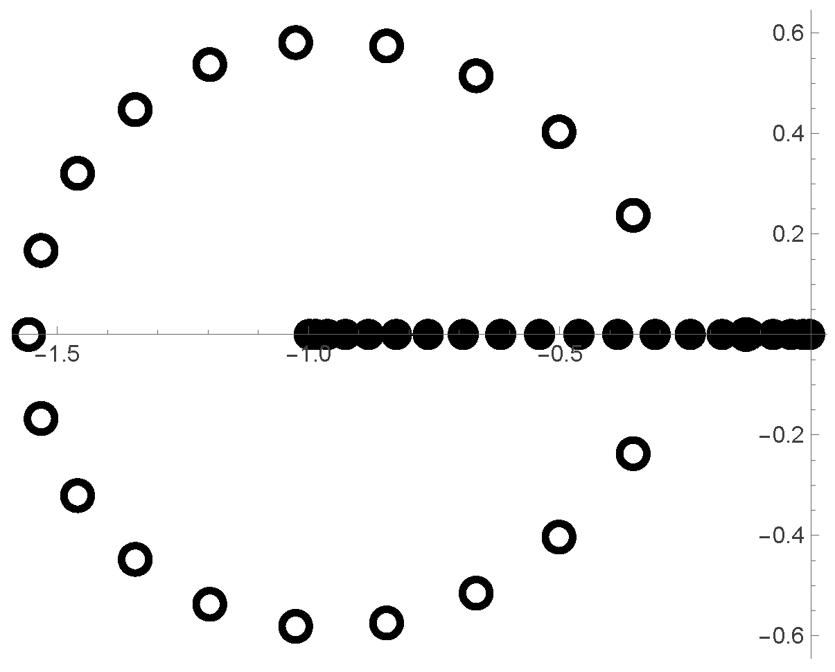
If not, it is worth giving a few numerical simulations aimed at confirming our conjecture about the action of the differential operator in Equation (33). To this end, in Figure 1, the spatial distribution, across the complex plane, of the zeros of the polynomial ${\mathcal{P}}_k\left(z\right)$ are shown (open circles) for $k=20$ and for the pair $(\alpha ,\gamma )=\left(1,{\displaystyle \frac{3}{2}}\right)$. In the same figure, the locations of ${\mathcal{Q}}_k\left(z\right)$’s zeros are also reported (dots), with all of them being real.

In order to provide a clear visual and numerical perspective of the mechanism proposed in Section 3, we are going to show the action of the derivative operator in Equation (33) through the auxiliary polynomial, say ${\mathcal{R}}_{k,m}\left(z\right)$, defined as

$$\begin{array}{c}{\displaystyle {\mathcal{R}}_{k,m}\left(z\right)={\displaystyle \frac{{\mathrm{d}}^m}{\mathrm{d}{z}^m}}\left\{z^{k-1}{\mathcal{P}}_k\left(z\right)\right\},m=1,2,\dots k-1.}\hfill \end{array}$$

(53)

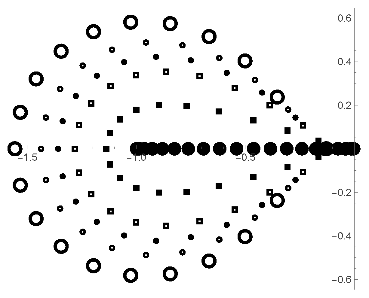
In this framework, the kth-order $\delta$-approximant denominator is reached just at the highest derivative order, i.e., ${\mathcal{Q}}_k\left(z\right)={\mathcal{R}}_{k,k-1}\left(z\right)$. Figure 2 illustrates the evolutionary process: the complex zero distributions of the polynomial ${\mathcal{R}}_{k,m}\left(z\right)$ defined in Equation (53), for low values of m, specifically $m=3$ (small open circles) and $m=5$ (small black circles), are plotted together with the initial distribution of the zeros of ${\mathcal{P}}_k\left(z\right)$ of Figure 1 (large open circles). Consistent with the Gauss–Lucas theorem, each differentiation step restricts the convex hull of these zeros and eventually, on further increasing the order to $m=7$ (small open squares), to $m=11$ (small black squares), and finally to $m=k-1=19$ (large black circles), confines them to the negative real half-axis.

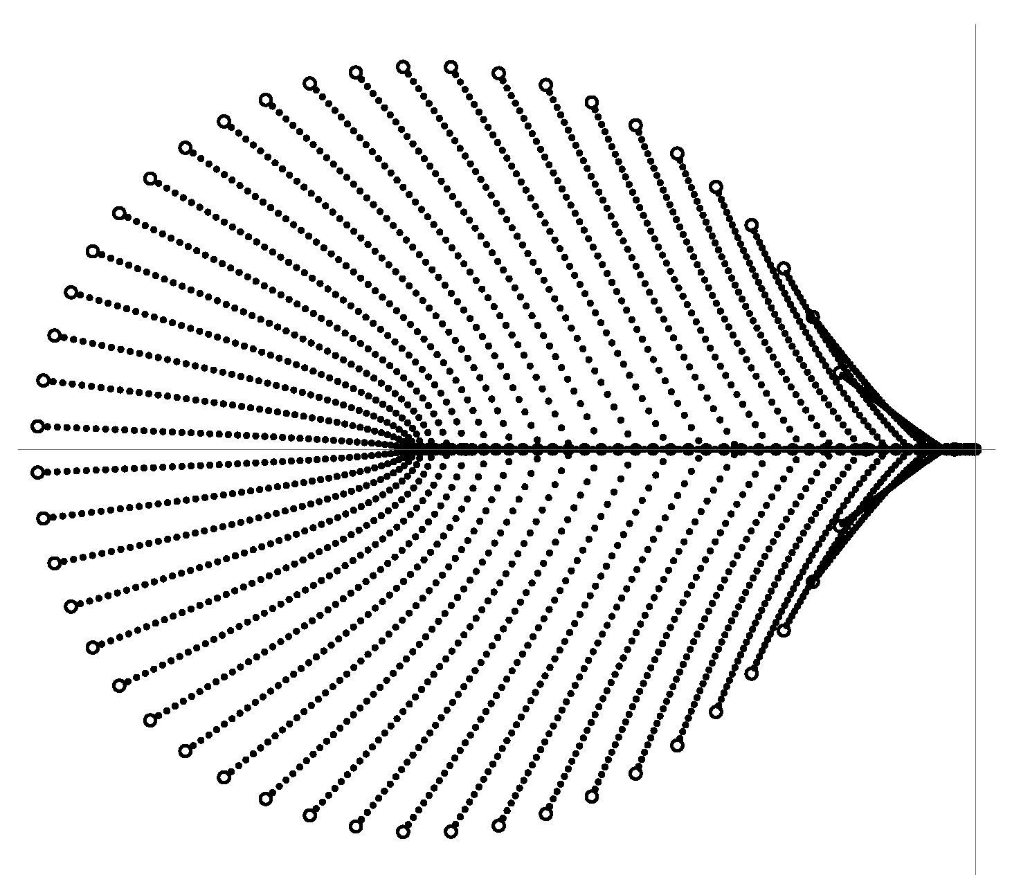
While the macroscopic restriction of the convex hull provides a solid geometrical interpretation of the $\delta$-approximant pole alignment, it could be instructive to examine this process from a different, ’dynamical’ perspective. This is achieved by tracking the individual ’motion’ of each zero as the differentiation order m increases, precisely in the form of precise trajectories in the complex plane that would bridge the gap between the initial complex-conjugated positions (open circles) and the final real axis destination (black circles). This complementary viewpoint would shift the focus from the global boundary of the zero set to the local evolution of its members. To give an example of this new perspective, Figure 3 shows the same as in Figure 2 but for the couple $(\alpha ,\gamma )=\left(1,1+{\displaystyle \frac{\pi }{3}}\right)$ and $k=50$. The plot now tracks the evolution of individual zeros as the differentiation order m runs in Equation (53) in the whole integer interval $[1,50]$. Within the global zero distributions made by small dots, the trajectories of each initial complex zero of ${\mathcal{P}}_k\left(z\right)$ (open circles) to its final real location (black circles) can be easily identified in the form of dotted curves. This visualization complements the convex hull analysis of Figure 2, and shows that the iterative differentiation forces each individual zero to follow a stable trajectory toward the Stieltjes branch cut. Numerous additional numerical simulations have been carried out, with the help of Wolfram Mathematica 14.3, for different values of k and $(\alpha ,\gamma )$, all of them systematically confirming our conjecture that all zeros of ${\mathcal{Q}}_k\left(z\right)$ in Equation (52) are real.

4.7. The Bessel Solution of Kepler’s Equation

The last example we are going to deal with is purely numerical. In a recent paper [5], a very classical and old problem was tackled from a new perspective. The problem consists in solving the following trascendental equation with respect to the unknown $\psi$:

$$M=\psi -ϵsin\psi ,$$

(54)

where $M\in [0,\pi ]$ and $ϵ\in [0,1]$ are real positive parameters. Equation (54) is the celebrated elliptic Kepler equation, playing a central role in Celestial Mechanics [58]. Among hundreds of different methods that have been conceived over more than four centuries to solve Kepler’s equation [4], in Ref. [5], the following Fourier series solution, originally proposed by Friedrich Wilhelm Bessel,

$$\begin{array}{c}{\displaystyle \psi =M+S(ϵ;M),}\hfill \end{array}$$

(55)

where [4] (Chapter 3)

$$\begin{array}{c}{\displaystyle S(ϵ;M)=\sum _{n=1}^{\infty }\frac{2J_n\left(nϵ\right)}{n}sinnM,}\hfill \end{array}$$

(56)

has been addressed under a new perspective. After introducing the complex function $\mathbb{S}(ϵ;M)$, defined through the Kapteyn series

$$\begin{array}{c}{\displaystyle \mathbb{S}(ϵ;M)=\sum _{n=1}^{\infty }\frac{2J_n\left(nϵ\right)}{n}exp\left(\mathrm{i}nM\right),}\hfill \end{array}$$

(57)

in such a way that $S=\mathrm{Im}\left\{\mathbb{S}\right\}$, it was shown that $\mathbb{S}(ϵ,M)$ is a Stieltjes series [5]. In particular, on introducing the parameter $\lambda <0$, defined as

$$\begin{array}{c}{\displaystyle \lambda =\chi +{\displaystyle \frac{1}{2}}log{\displaystyle \frac{1-\chi }{1+\chi }},}\hfill \end{array}$$

(58)

where $\chi =\sqrt{1-{ϵ}^2}$, it was proved that the function $\mathbb{S}(ϵ,M)$ defined in Equation (57) is a Stieltjes series characterized by the following moment sequence [5]:

$${\mu }_n={\displaystyle \frac{2J_{n+1}\left[(n+1)ϵ\right]}{(n+1)}}exp\left[-\lambda (n+1)\right],n\in {\mathbb{N}}_0.$$

(59)

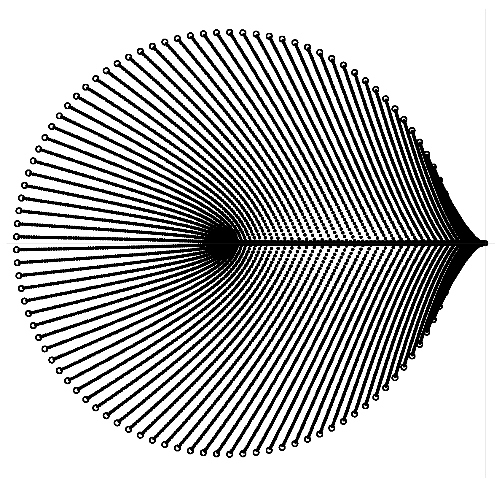
Differently from the case of Jacobi’s distribution, in the present case it is no longer possible to express either ${\mathcal{P}}_k\left(z\right)$ or ${\mathcal{Q}}_k\left(z\right)$ in closed form. Nevertheless, numerical experiments carried out with the aid of Wolfram Mathematica 14.3 confirm the robustness of our approach. To illustrate it, Figure 4 examines the zero trajectories for $ϵ=99/100$ and for $k=100$. This large-scale simulation highlights the power of the iterated differentiation mechanism: even starting from a dense set of 100 initial complex zeros, the trajectories show their systematic migration toward the real negative half-axis. Several other simulations, not shown here, have confirmed the main conjecture of the present paper also for high-order $\delta$-approximants of the Stieltjes series $\mathbb{S}(ϵ,M)$ defined in Equation (57).

5. Conclusions

Nonlinear sequence transformations in general, and Weniger’s $\delta$-transformation in particular, are nowadays considered computational tools of great importance for the resummation of several divergent series occurring in applied mathematics as well as in theoretical physics.

For Stieltjes series, a complete convergence theory already exists, as far as their resummation is concerned, via Padé approximants. In particular, the reality and negativity of the poles have been rigorously established (see Ref. [7]). In the present work, we have addressed the capability of correctly simulating the branch cut of a typical Stieltjes function when the Weniger transformation is applied to the corresponding Stieltjes asymptotic series. Our investigation has been constructed as a two-step procedure. First, we have demonstrated that the log-convexity of a typical Stieltjes moment sequence guarantees the validity of the necessary condition for any $\delta$-approximant pole to be real. Subsequently, we have shown that the denominator of a kth-order $\delta$-approximant can always be recast as the $(k-1)$th-order derivative of the polynomial $z^{k-1}{\mathcal{P}}_k\left(z\right)$, where the log-concave polynomial ${\mathcal{P}}_k\left(z\right)$ is a binomial sum containing the inverse of $k+1$ consecutive Stieltjes series moments. In this way, the Gauss–Lucas theorem has been utilized to visualize the iterative action of the differentiation operator, which forces the convex hull of the zeros to be progressively restricted toward the negative real axis.

Since a fully rigorous proof of our conjecture remains an open challenge, an extensive numerical exploration of the mechanism that produces the correct branch cut scenario has been proposed. Several simulations, carried out on a broad catalog of Stieltjes series (including superfactorially divergent ones), systematically confirmed our conjecture. Figure 3 and Figure 4 represent the cornerstone of such numerical exploration. In the latter, by tracking the migration of 50 and 100 individual poles via Equation (53), the aligning power of the differentiation approach is highlighted as a robust structural property. The visual evidence of a dense web of complex trajectories perfectly collapsing onto the negative real axis provides a compelling justification for our conjecture, bridging the gap between theoretical intuition and systematic evidence. However, a fully rigorous proof still remains an outstanding open challenge which, once solved, would close this gap and would finally place Levin-type transformations on the same rigorous footing as the classical Padé approximants, as far as Stieltjes series resummation is concerned.

References

1. Bender, C.M.; Weniger, E.J. Numerical evidence that the perturbation expansion for a non-Hermitian PT-symmetric Hamiltonian is Stieltjes. J. Math. Phys. 2001, 42, 2167–2183. [Google Scholar]
2. Grecchi, V.; Maioli, M.; Martinez, A. Padé summability of the cubic oscillator. J. Phys. A 2009, 42, 425208. [Google Scholar]
3. Grecchi, V.; Martinez, A. The spectrum of the cubic oscillator. Commun. Math. Phys. 2013, 319, 479–500. [Google Scholar]
4. Colwell, P. Solving Kepler’s Equation Over Three Centuries; Willmann-Bell: Richmond, VA, USA, 1993. [Google Scholar]
5. Borghi, R. On the Bessel Solution of Kepler’s Equation. Mathematics 2024, 12, 154. [Google Scholar] [CrossRef] [Scilit]
6. Wynn, P. On a device for computing the em(Sn) transformation. Math. Tables Aids Comput. 1956, 10, 91–96. [Google Scholar]
7. Baker, G.A., Jr.; Graves-Morris, P. Padé Approximants, 2nd ed.; Cambridge U. P.: Cambridge, UK, 1996. [Google Scholar]
8. Graffi, S.; Grecchi, V. Borel summability and indeterminacy of the Stieltjes moment problem: Application to the anharmonic oscillators. J. Math. Phys. 1978, 19, 1002–1006. [Google Scholar] [CrossRef] [Scilit]
9. Weniger, E.J. A convergent renormalized strong coupling perturbation expansion for the ground state energy of the quartic, sextic, and octic anharmonic oscillator. Ann. Phys. 1996, 246, 133–165. [Google Scholar] [CrossRef] [Scilit]
10. Weniger, E.J. Construction of the strong coupling expansion for the ground state energy of the quartic, sextic and octic anharmonic oscillator via a renormalized strong coupling expansion. Phys. Rev. Lett. 1996, 77, 2859–2862. [Google Scholar] [CrossRef] [Scilit] [PubMed]
11. Borghi, R. Factorial Series Representation of Stieltjes Series Converging Factors. Mathematics 2024, 12, 2330. [Google Scholar] [CrossRef] [Scilit]
12. Weniger, E.J. Nonlinear sequence transformations for the acceleration of convergence and the summation of divergent series. Comput. Phys. Rep. 1989, 10, 189–371. [Google Scholar] [CrossRef] [Scilit]
13. Borghi, R. Converging Factors of a Class of Superfactorially Divergent Stieltjes Series. Mathematics 2025, 13, 2974. [Google Scholar] [CrossRef] [Scilit]
14. Borghi, R.; Weniger, E.J. Convergence analysis of the summation of the factorially divergent Euler series by Padé approximants and the delta transformation. Appl. Numer. Math. 2015, 94, 149–178. [Google Scholar] [CrossRef] [Scilit]
15. Henrici, P. Applied and Computational Complex Analysis II; Wiley: New York, NY, USA, 1977. [Google Scholar]
16. Euler, L. Institutiones Calculi Differentialis Cum Eius Usu in Analysi Finitorum Ac Doctrina Serierum. Pars II.1. De Transformatione Serierum; Academia Imperialis Scientiarum Petropolitana: St. Petersburg, Russia, 1755; reprinted in Leonardi Euleri Opera Omnia, Seria Prima; Teubner: Leipzig, Germany; Berlin, Germany, 1913. [Google Scholar]
17. Brezinski, C.; Redivo Zaglia, M. Extrapolation Methods; North-Holland: Amsterdam, The Netherlands, 1991. [Google Scholar]
18. Airey, J.R. The “converging factor” in asymptotic series and the calculation of Bessel, Laguerre and other functions. Philos. Mag. 1937, 24, 521–552. [Google Scholar]
19. Dingle, R.B. Asymptotic Expansions: Their Derivation and Interpretation; Academic Press: London, UK, 1973. [Google Scholar]
20. Shanks, D. Non-linear transformations of divergent and slowly convergent sequences. J. Math. Phys. 1955, 34, 1–42. [Google Scholar]
21. Olver, F.W.J.; Lozier, D.W.; Boisvert, R.F.; Clark, C.W. (Eds.) NIST Handbook of Mathematical Functions; Cambridge U. P.: Cambridge, UK, 2010. [Google Scholar]
22. Levin, D. Development of non-linear transformations for improving convergence of sequences. Int. J. Comput. Math. B 1973, 3, 371–388. [Google Scholar]
23. Weniger, E.J. Mathematical properties of a new Levin-type sequence transformation introduced by Čížek, Zamastil, and Skála. I. Algebraic theory. J. Math. Phys. 2004, 45, 1209–1246. [Google Scholar] [CrossRef] [Scilit]
24. Weniger, E.J. Summation of divergent power series by means of factorial series. Appl. Numer. Math. 2010, 60, 1429–1441. [Google Scholar] [CrossRef] [Scilit]
25. Weniger, E.J.; Steinborn, E.O. Nonlinear sequence transformations for the efficient evaluation of auxiliary functions for GTO molecular integrals. In Proceedings of the Numerical Determination of the Electronic Structure of Atoms, Diatomic and Polyatomic Molecules, Versailles, France, 17–22 April 1988; Defranceschi, M., Delhalle, J., Eds.; NATO ASI Series; Kluwer: Dordrecht, The Netherlands, 1989; pp. 341–346. [Google Scholar]
26. Jentschura, U.D.; Gies, H.; Valluri, S.R.; Lamm, D.R.; Weniger, E.J. QED effective action revisited. Can. J. Phys. 2002, 80, 267–284. [Google Scholar] [CrossRef] [Scilit]
27. Jentschura, U.D.; Lötstedt, E. Numerical calculation of Bessel, Hankel and Airy functions. Comput. Phys. Commun. 2012, 183, 506–519. [Google Scholar] [CrossRef] [Scilit]
28. Jentschura, U.D.; Mohr, P.J.; Soff, G.; Weniger, E.J. Convergence acceleration via combined nonlinear-condensation transformations. Comput. Phys. Commun. 1999, 116, 28–54. [Google Scholar] [CrossRef] [Scilit]
29. Weniger, E.J. On the summation of some divergent hypergeometric series and related perturbation expansions. J. Comput. Appl. Math. 1990, 32, 291–300. [Google Scholar] [CrossRef] [Scilit]
30. Weniger, E.J. Interpolation between sequence transformations. Numer. Algorithms 1992, 3, 477–486. [Google Scholar] [CrossRef] [Scilit]
31. Weniger, E.J. On the efficiency of linear but nonregular sequence transformations. In Nonlinear Numerical Methods and Rational Approximation II; Cuyt, A., Ed.; Kluwer: Dordrecht, The Netherlands, 1994; pp. 269–282. [Google Scholar]
32. Weniger, E.J. Computation of the Whittaker function of the second kind by summing its divergent asymptotic series with the help of nonlinear sequence transformations. Comput. Phys. 1996, 10, 496–503. [Google Scholar] [CrossRef] [Scilit]
33. Weniger, E.J. Irregular input data in convergence acceleration and summation processes: General considerations and some special Gaussian hypergeometric series as model problems. Comput. Phys. Commun. 2001, 133, 202–228. [Google Scholar] [CrossRef] [Scilit]
34. Weniger, E.J. On the analyticity of Laguerre series. J. Phys. A 2008, 41, 425207. [Google Scholar] [CrossRef] [Scilit]
35. Weniger, E.J.; Čížek, J. Rational approximations for the modified Bessel function of the second kind. Comput. Phys. Commun. 1990, 59, 471–493. [Google Scholar] [CrossRef] [Scilit]
36. Čížek, J.; Vinette, F.; Weniger, E.J. Examples on the use of symbolic computation in physics and chemistry: Applications of the inner projection technique and of a new summation method for divergent series. Int. J. Quantum Chem. Symp. 1991, 25, 209–223. [Google Scholar]
37. Čížek, J.; Vinette, F.; Weniger, E.J. On the use of the symbolic language Maple in physics and chemistry: Several examples. In Proceedings of the Fourth International Conference on Computational Physics PHYSICS COMPUTING ’92, Prague, Czech Republic, 24–28 August 1992; de Groot, R.A., Nadrchal, J., Eds.; World Scientific: Singapore, 1993; pp. 31–44. [Google Scholar]
38. Čížek, J.; Vinette, F.; Weniger, E.J. On the use of the symbolic language Maple in physics and chemistry: Several examples. Int. J. Mod. Phys. C 1993, 4, 257–270. [Google Scholar] [CrossRef] [Scilit]
39. Caliceti, E.; Meyer-Hermann, M.; Ribeca, P.; Surzhykov, A.; Jentschura, U.D. From useful algorithms for slowly convergent series to physical predictions based on divergent perturbative expansions. Phys. Rep. 2007, 446, 1–96. [Google Scholar] [CrossRef] [Scilit]
40. Čížek, J.; Zamastil, J.; Skála, L. New summation technique for rapidly divergent perturbation series. Hydrogen atom in magnetic field. J. Math. Phys. 2003, 44, 962–968. [Google Scholar] [CrossRef] [Scilit]
41. Jentschura, U.D.; Becher, J.; Weniger, E.J.; Soff, G. Resummation of QED perturbation series by sequence transformations and the prediction of perturbative coefficients. Phys. Rev. Lett. 2000, 85, 2446–2449. [Google Scholar] [CrossRef] [Scilit]
42. Jentschura, U.D.; Weniger, E.J.; Soff, G. Asymptotic improvement of resummations and perturbative predictions in quantum field theory. J. Phys. G 2000, 26, 1545–1568. [Google Scholar] [CrossRef] [Scilit]
43. Weniger, E.J. Nonlinear sequence transformations: A computational tool for quantum mechanical and quantum chemical calculations. Int. J. Quantum Chem. 1996, 57, 265–280, Erratum in Int. J. Quantum Chem. 1996, 58, 319–321. [Google Scholar] [CrossRef]
44. Weniger, E.J. Performance of superconvergent perturbation theory. Phys. Rev. A 1997, 56, 5165–5168. [Google Scholar] [CrossRef] [Scilit]
45. Weniger, E.J.; Čížek, J.; Vinette, F. Very accurate summation for the infinite coupling limit of the perturbation series expansions of anharmonic oscillators. Phys. Lett. A 1991, 156, 169–174. [Google Scholar] [CrossRef] [Scilit]
46. Weniger, E.J.; Čížek, J.; Vinette, F. The summation of the ordinary and renormalized perturbation series for the ground state energy of the quartic, sextic, and octic anharmonic oscillators using nonlinear sequence transformations. J. Math. Phys. 1993, 34, 571–609. [Google Scholar] [CrossRef] [Scilit]
47. Borghi, R.; Santarsiero, M. Summing Lax series for nonparaxial beam propagation. Opt. Lett. 2003, 28, 774–776. [Google Scholar] [CrossRef] [Scilit]
48. Li, J.X.; Zang, W.; Li, Y.D.; Tian, J. Acceleration of electrons by a tightly focused intense laser beam. Opt. Express 2009, 17, 11850–11859. [Google Scholar] [CrossRef] [Scilit] [PubMed]
49. Li, J.; Zang, W.; Tian, J. Simulation of Gaussian laser beams and electron dynamics by Weniger transformation method. Opt. Express 2009, 17, 4959–4969. [Google Scholar] [CrossRef] [Scilit] [PubMed]
50. Dai, L.; Li, J.X.; Zang, W.P.; Tian, J.G. Vacuum electron acceleration driven by a tightly focused radially polarized Gaussian beam. Opt. Express 2011, 19, 9303–9308. [Google Scholar] [CrossRef] [Scilit]
51. Borghi, R.; Gori, F.; Guattari, G.; Santarsiero, M. Decoding divergent series in nonparaxial optics. Opt. Lett. 2011, 36, 963–965. [Google Scholar] [CrossRef] [Scilit]
52. Borghi, R. Evaluation of diffraction catastrophes by using Weniger transformation. Opt. Lett. 2007, 32, 226–228. [Google Scholar] [CrossRef] [Scilit] [PubMed]
53. Borghi, R. Numerical computation of diffraction catastrophes with codimension eight. Phys. Rev. E 2012, 85, 046704. [Google Scholar] [CrossRef] [Scilit] [PubMed]
54. Rahman, Q.I.; Schmeisser, G. Analytic Theory of Polynomials; Clarendon Press: Oxford, UK, 2003. [Google Scholar]
55. Richards, D. Totally positive kernels, Polýa frequency functions, and generalized hypergeometric series. Linear Algebra Its Appl. 1990, 137–138, 467–478. [Google Scholar] [CrossRef] [Scilit]
56. Schoenberg, I.J. On Pólya frequency functions. I. The totally positive functions and their Laplace transforms. J. d’Anal. Math. 1951, 1, 331–374. [Google Scholar] [CrossRef] [Scilit]
57. Driver, K.; Jordaan, K.; Martínez-Finkelshtein, A. Pólya frequency sequences and real zeros of some 3F2 polynomials. J. Math. Anal. Appl. 2007, 332, 1045–1055. [Google Scholar] [CrossRef] [Scilit]
58. Orlando, F.; Farina, C.; Zarro, C.; Terra, P. Kepler’s equation and some of its pearls. Am. J. Phys. 2018, 86, 849–858. [Google Scholar] [CrossRef] [Scilit]
Figure 1. Locations, on the complex plane, of the zeros of the polynomial P k ( z ) (open circles) and of the polynomial Q k ( z ) (black circles), for k = 20 and for the pair ( α , γ ) = 1 , 3 2 .
Mathematics 14 00376 g001
Figure 2. The same as in Figure 1, but now the plot illustrates also the distributions of zeros for the intermediate polynomials R k , m ( z ) defined in Equation (53) for m = 3 (small open circles), m = 5 (small black circles), m = 7 (small open squares), and m = 11 (small black squares). Consistent with the Gauss–Lucas theorem, each differentiation step constrains the new zeros within the convex hull of the previous set.
Mathematics 14 00376 g002
Figure 3. The same as in Figure 2, but for the couple ( α , γ ) = 1 , 1 + π 3 and for the δ -approximant order k = 50 . The plot now tracks the individual evolution of zeros across the complex plane as the differentiation order m runs in Equation (53) in the whole integer interval [ 1 , 50 ] .
Mathematics 14 00376 g003
Figure 4. The same as in Figure 3, but for the Stieltjes series S ( ϵ , M ) defined in Equation (57), evaluated at ϵ = 99 / 100 and k = 100 . The individual evolution of 100 zeros are tracked as the differentiation order increases. Open circles represent the initial zeros of P 100 ( z ) , while black circles denote the final poles of the corresponding δ -approximant.
Mathematics 14 00376 g004
Disclaimer/Publisher’s Note: The statements, opinions and data contained in all publications are solely those of the individual author(s) and contributor(s) and not of MDPI and/or the editor(s). MDPI and/or the editor(s) disclaim responsibility for any injury to people or property resulting from any ideas, methods, instructions or products referred to in the content.