An Improved Similarity Measure for Interval-Valued Intuitionistic Fuzzy Numbers and Its Application to Multi-Attribute Decision-Making Problem

Abstract

In this article, a new similarity measure is discussed on interval-valued intuitionistic fuzzy values (IVIFVs). Here, the proposed similarity measure has been derived based on transformed intervals and its probability density functions, mean values, and standard deviations of IVIFVs. Based on the proposed similarity measure, several essential properties have been illustrated in this paper. Additionally, a new algorithm has been developed using the similarity measure of interval-valued intuitionistic fuzzy values (IVIFVs) to solve multi-attribute decision-making (MADM) problem. The proposed method is highly effective for solving various types of MADM problems. To demonstrate the effectiveness of the proposed similarity measure, a car selection problem has been considered, where the objective is to choose a suitable car for a decision maker from a set of alternatives evaluated under multiple criteria. In car selection, different features often involve conflicting criteria with imprecise data. Therefore, the proposed similarity measure of interval-valued intuitionistic fuzzy values assists in determining the best alternative among these conflicting criteria.

1. Introduction

Uncertainty in many real-life problems is effectively determined using fuzzy set theory, which was first introduced by [1]. Since its invention, various developments in fuzzy set theory have been proposed by various researchers. Over the past few decades, similarity measures for different types of fuzzy numbers have been extensively studied and applied to a wide range of real-life decision-making problems. So, because of the greatest potentiality of similarity measures, many researchers have focused on developing similarity measures for various types of fuzzy numbers.

In 2003, ref. [2] presented a similarity measure between fuzzy numbers based on distance and the center of gravity. Ref. [3] developed a fuzzy similarity measure for interval-valued fuzzy numbers. Using linguistic term values, ref. [4] proposed a new similarity measure for generalized trapezoidal fuzzy numbers and applied it to a fuzzy risk analysis problem. In 2010, ref. [5] introduced another method for measuring similarity between trapezoidal fuzzy numbers. Later, ref. [6] proposed a similarity measure between two generalized trapezoidal fuzzy numbers based on area and perimeter. In 2015, ref. [7] introduced an area and height-based similarity measure for generalized trapezoidal fuzzy numbers. Furthermore, in 2016, ref. [8] proposed a similarity measure for interval-valued fuzzy numbers.

In the real world, there is vast application of similarity measures in multi-attribute decision-making (MADM) problems. These kinds of problem solely depend on the choice of the decision maker. Therefore, the choice of alternatives is fully decided by a decision maker. However, the chosen value of some attributes is not always a crisp value. Therefore, the choice becomes more complicated. As it is not crisp, it may be considered to have a fuzzy nature. Thus, the choice parameters of any decision maker have some positive impacts as well as negative impacts for each alternative. Therefore, intuitionistic fuzzy numbers are very useful in such cases.

Intuitionistic fuzzy sets and their properties were first proposed by [9]. Nowadays, intuitionistic fuzzy numbers draw great attention from some researchers due to their widespread applicability in real-life problems to measure the similarity. There has also been some studies on intuitionistic fuzzy numbers. In 2012, ref. [10] introduced a multi-criteria group decision-making method using a vector similarity measure for trapezoidal intuitionistic fuzzy numbers. Also, ref. [11] proposed a similarity measure using the Hamming distance and the Euclidean distance between trapezoidal intuitionistic fuzzy numbers.Then, a new similarity measure of generalized trapezoidal intuitionistic fuzzy numbers and generalized interval-valued fuzzy numbers was developed by [12] in 2013. After that in 2017, ref. [13] proposed a similarity measure of intuitionistic fuzzy numbers and its application to clustering. Also, many other decision-making problems have been analyzed using intuitionistic fuzzy set theory.

Interval-valued intuitionistic fuzzy sets were introduced by [14], each of which is characterized by a membership function and a non-membership function whose values are intervals rather than exact numbers, and are a very useful means to describe decision information in the decision-making process. Some researchers have applied the interval-valued intuitionistic fuzzy set theory to the field of decision-making. Ref. [15] proposed a networked control system with an interval type-2 fuzzy set and applied it in deception attacks in dual communication channels.

Now, similarity measures have numerous applications in various decision-making problems. Multi-attribute decision-making (MADM) problems have been studied by different researchers using interval-valued intuitionistic fuzzy values (IVIFVs) at different times. In recent years, a significant number of studies have focused on MADM problems using IVIFVs. Ref. [16] developed a method for an interval-valued intuitionistic fuzzy (IVIF) MADM based on the particle swarm optimization (PSO) methodology and evidential reasoning approach. Using the U-quadratic distribution, ref. [17] developed a method for IVIF MADM with the help of the transformed decision matrix (TDM). Ref. [18] developed a new method for IVIF MADM that is based on probability density functions (PDFs). Ref. [19] developed a new method on the basis of interval-valued intuitionistic fuzzy values (IVIFVs) for MADM. Using the linear programming (LP) techniques, ref. [20] developed a method for MADM on the basis of IVIFVs. An MADM method was presented by [21] with the help of nonlinear programming (NLP) techniques, particle swarm optimization (PSO) techniques and IVIFVs. In 2017, ref. [22] proposed an MADM method with the use of IVIFVs and LP techniques. Ref. [23] developed an MADM method based on IVIFVs and PSO techniques. In 2018, ref. [24] introduced an MADM method that was based on NLP techniques with hyperbolic functions and IVIFVs. Based on Shannon’s information entropy, NLP techniques and IVIFVs, ref. [25] proposed an MADM method. Ref. [26] proposed an MADM method based on IVIFSs. For hotel selection, an MADM was presented by [27] for IVIFSs. TOPSIS-based nonlinear-programming methodology has been applied to multi-attribute decision-making problems with IVIFSs by [28]. Ref. [29] proposed an MADM method based on IVIFSs. Using transform decision matrix in IVIFSs and with PDFs, an MADM was presented by [30]. Ref. [31] presented an MADM method using a possibility measure of IVIFSs and connection numbers of SPA. Based on divergence measures for multi-criteria assessment of programming language with IVIFSs, Mishra et al. [32] established an extended MABAC method.

Kumar and Chen [33] proposed an MADM based on converted decision matrices (CDM), PDF and IVIFV. Ref. [34] developed an MADM method based on IVIFVs. Ref. [35] explored a new ranking method to evaluate the risk of diabetes problems using generalized trapezoidal fuzzy numbers. Ref. [36] developed a new ranking method for generalized trapezoidal fuzzy numbers and applied it in a fuzzy risk analysis problem. Using fuzzy preference relations of incomplete interval-valued linguistic intuitionistic fuzzy numbers, a group decision-making method was developed by [37]. This paper deals with incomplete information and develops an optimization model in decision-making problems.

From the above literature review, it is seen that similarity does not exist among the IVIFVs. So, the following questions arise:

• What will the similarity of the IVIFVs be for different IVIFVs?
• If one has to choose an alternative from a set of alternatives, whose criteria are given in the form of IVIFVs?

So, our objective is to solve these questions under the imprecise environment. This motivates us to introduce a new similarity measure technique for IVIFVs and also to develop an MAMD problem whose data are of the form of IVIFVs.

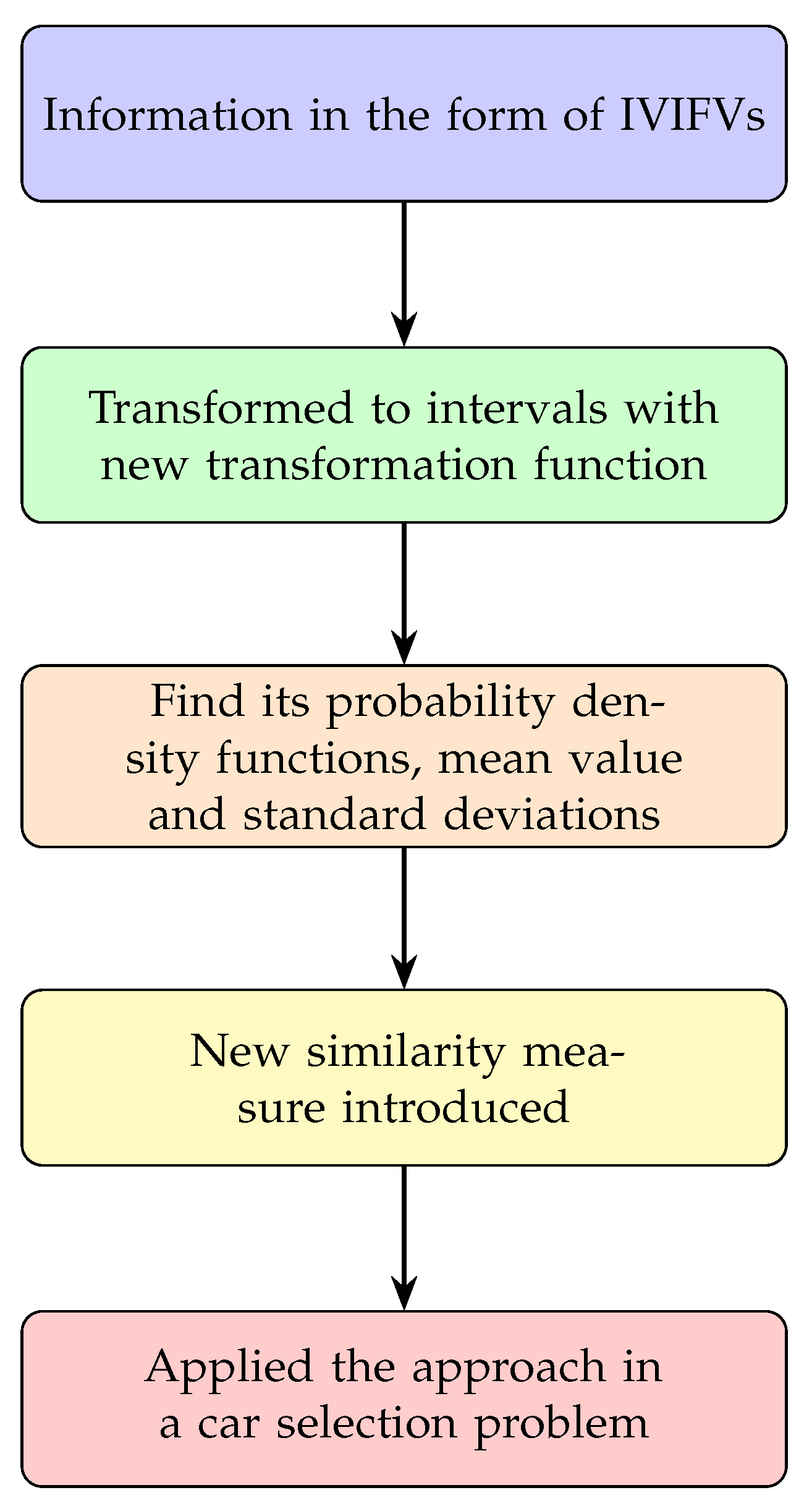
So, in this paper, a new approach to similarity measures is proposed for IVIFVs that is based on transformed intervals and the probability density functions, mean value and standard deviations of IVIFVs. Depending on the proposed method of similarity measures, some essential properties are illustrated in this paper. Also, a new algorithm is developed using the similarity measure of IVIFVs for solving multi-attribute decision-making (MADM) problems, and to show the effectiveness of the proposed similarity measure, a car selection problem is considered to select a suitable car for a decision maker from a set of cars with different criteria. A flowchart of the proposed work is provided in the following Figure 1.

This paper is organized as follows. In Section 2, we introduce the preliminaries of IVIFVs. In Section 3, a new method for similarity measures of IVIFVs is proposed and some properties regarding the proposed similarity measure are derived. A new algorithmic approach to solving the MADM problem using similarity measures of IVIFVs has been discussed in Section 4. In Section 5, for numerical illustration, a car selection problem has been considered in which a decision maker must select a suitable car from a set of cars with different criteria, evaluated with the proposed similarity measure technique. In Section 6, the conclusion is presented.

2. Some Preliminaries on Similarity Measure of IVIFVs

In this section, some definitions, concepts and arithmetic operations of IVIFVs are discussed. We provide some basic definitions of fuzzy sets, intuitionistic fuzzy sets, interval-valued intuitionistic fuzzy sets, interval-valued intuitionistic fuzzy values and the 68-95-99.7 rule.

Definition 1

(Fuzzy Set: ([1])).  A fuzzy set $\tilde{A}$ in the universe of discourse X is defined by

$$\tilde{A}=\left\{(x,{\mu }_A\left(x\right))\right|x\in X\}$$

where ${\mu }_A\left(x\right)$ denotes the membership grade of x to $\tilde{A}$, $x\in X$, $0\le {\mu }_A\left(x\right)\le 1$.

Definition 2

(Intuitionistic Fuzzy Set: ([9])). An IFS $\tilde{A}$ in the universe of discourse X is defined by

$$\tilde{A}=\{<x,{\mu }_A\left(x\right),{\nu }_A\left(x\right)>|x\in X\}$$

where ${\mu }_A\left(x\right)$ and ${\nu }_A\left(x\right)$ denote the membership grade and the non-membership grade of x to $\tilde{A}$, respectively, $x\in X$, $0\le {\mu }_A\left(x\right)\le {\nu }_A\left(x\right)\le 1$.

Definition 3

(Interval-Valued Intuitionistic Fuzzy Set and IVIFV: ([14])). An IVIFS $\tilde{A}$ in the universe of discourse X is defined by

$$\tilde{A}=\{<x,[{\tau }_A\left(x\right),{\eta }_A\left(x\right)],[{\theta }_A\left(x\right),{\nu }_A\left(x\right)]>|x\in X\}$$

where $[{\tau }_A\left(x\right),{\eta }_A\left(x\right)]$ and $[{\theta }_A\left(x\right),{\nu }_A\left(x\right)]$ denote the interval-valued membership grade and the interval-valued non-membership grade of x to $\tilde{A}$, respectively, $x\in X$, $0\le {\tau }_A\left(x\right)\le {\eta }_A\left(x\right)\le 1$ and $0\le {\theta }_A\left(x\right)\le {\nu }_A\left(x\right)\le 1$.

In [5], Xu denotes the pair $<[\tau ,\eta ][\theta ,\nu ]>$ as IVIFV, where $0\le \tau \le \eta \le 1$ and $0\le \theta \le \nu \le 1$.

Definition 4

(68-95-99.7 rule: ([33])). The 68-95-99.7 rule, empirical rule or three-sigma rule is a statistical rule that states that for a normal distribution, almost the entire observed dataset will lie within three standard deviations (σ) of the mean (μ). Particularly, $68.27\%$ of the data lie within one SD of the mean, $95.45\%$ of the data lie within two SDs of the mean and $99.73\%$ of the data lie within three SDs of the mean.

3. The Novel Approach Similarity Measure Using IVIFV

Let $X_1=<[{\tau }_1,{\eta }_1],[{\theta }_1,{\upsilon }_1]>$ and $X_2=<[{\tau }_2,{\eta }_2],[{\theta }_2,{\upsilon }_2]>$ be two IVIFVs. Here, the membership grades and non-membership grades of the IVIFVs are interval-valued. So, they are quite difficult to compare directly. To remove this difficulty, at first, we convert the IVIFVs to the membership interval values using some proper transformation and then determine the similarity among them. The process of finding the proposed similarity measure is discussed in the following algorithm. A new similarity measure between two IVIFVs has been formulated using the following algorithm:

Step 1: To convert the IVIFVs $X_1=<[{\tau }_1,{\eta }_1],[{\theta }_1,{\upsilon }_1]>$ and $X_2=<[{\tau }_2,{\eta }_2],[{\theta }_2,{\upsilon }_2]>$ into two intervals $[a_1,b_1]$ and $[a_2,b_2]$, the following transformation is proposed:

$$\begin{array}{ccc}& & a_i=\left({\displaystyle \frac{{\tau }_i+{\eta }_i}{2}}\right)\left[1-\left\{{\displaystyle \frac{{\eta }_i-{\tau }_i}{2}}\right\}\right]\hfill \\ & & b_i=1-\left[\left({\displaystyle \frac{{\theta }_i+{\upsilon }_i}{2}}\right)\left\{1-({\displaystyle \frac{{\upsilon }_i-{\theta }_i}{2}})\right\}\right]\hfill \end{array}$$

$i=1,2$.

Here, the transformation has been made in such a way that the transformed interval belongs to $[0,1]$. As the values of ${\tau }_i,{\eta }_i,{\theta }_i,{\upsilon }_i$ lie in the interval, from the transform equation it is easily seen that the the values of $a_i$ and $b_i$ lie within the interval $[0,1]$. So, it is obvious that the transformed interval is bounded.

Again, it is also seen that the value of $b_i$ is always greater or equals that of $a_i$.

Since, for an IVIFV, ${\tau }_i\le {\eta }_i$, ${\theta }_i\le {\upsilon }_i$ and ${\tau }_i+{\theta }_i\le 1$, ${\eta }_i+{\upsilon }_i\le 1$, this means that $b_i-a_i=1-{\displaystyle \frac{{\tau }_i+{\eta }_i+{\theta }_i+{\upsilon }_i}{2}}+{\displaystyle \frac{{\eta }_i^2-{\tau }_i^2}{2}}+{\displaystyle \frac{{\upsilon }_i^2-{\theta }_i}{2}}\ge 0.$

Hence, $b_i\ge a_i$.

Also, the transformation to $a_i,b_i$ follows its monotonicity, as with the increase in the value of ${\tau }_i,{\eta }_i$ the values of $a_i$ increase and with increases in the values in ${\theta }_i,{\upsilon }_i$, the values of $b_i$ decrease within the interval $[0,1]$.

Step 2: Now, the PDF $p_i\left(x\right)$ for each membership interval is calculated as follows:

$$\begin{array}{c}\hfill {\displaystyle p_i\left(x\right)=\frac{1}{\frac{b_i-a_i}{2}\sqrt{2\pi }}{e}^{\left(-\frac{{(x-\frac{b_i+a_i}{2})}^2}{2{\left(\frac{b_i-a_i}{2}\right)}^2}\right)}}\end{array}$$

$i=1,2$.

Step 3: Calculate the mean value of each interval as

$$\begin{array}{c}\hfill {\mu }_i=\left\{\begin{array}{cc}{\displaystyle {\int }_{a_i}^{b_i}x{p}_i\left(x\right)dx,}\hfill & \mathrm{if}{a}_i\ne b_i;\hfill \\ 0.6827\times b_i,\hfill & \mathrm{if}{a}_i=b_i.\hfill \end{array}\right.\end{array}$$

Step 4: Next, the variance $Va{r}_i$ is calculated for intervals as follows:

$$\begin{array}{c}\hfill Va{r}_i=\left\{\begin{array}{cc}{\displaystyle {\int }_{a_i}^{b_i}{(x-{\mu }_i)}^2{p}_i\left(x\right)dx,}\hfill & \mathrm{if}{a}_i\ne b_i;\hfill \\ 0.6827\times {(b_i-{\mu }_i)}^2,\hfill & \mathrm{if}{a}_i=b_i.\hfill \end{array}\right.\end{array}$$

Step 5: Calculate the SD for each interval as ${\sigma }_i=\sqrt{va{r}_i\left(x\right)}$.

Step 6: Calculate the mean difference as $\varphi =|{\mu }_1-{\mu }_2|$.

Step 7: Calculate the SD difference as $\psi =|{\sigma }_1-{\sigma }_2|$.

Step 8: Calculate the similarity measure $S(X_1,X_2)$ of $X_1$ and $X_2$ as $S(X_1,X_2)=1-{\left(\frac{{\varphi }^2+{\psi }^2}{2}\right)}^{\frac{1}{2}}$.

Example 1.

Let $X_1=<[0.5,0.5],[0.2,0.2]>$; $X_2=<[0.4,0.6],[0.1,0.3]>$ and $X_3=<[0.4,0.6],[0.1,0.2]>$ be three IVIFVs.

Here, $a_1=0.5$, $a_2=0.45$, $a_3=0.45$ and $b_1=0.8$, $b_2=0.82$, $b_3=0.8575$.

$$\begin{array}{c}\hfill {\displaystyle p_1\left(x\right)=\frac{1}{0.15\left(\sqrt{2\pi }\right)}{e}^{\left(-\frac{{(x-0.65)}^2}{2{\left(0.15\right)}^2}\right)}}\end{array}$$

$$\begin{array}{c}\hfill {\displaystyle p_2\left(x\right)=\frac{1}{0.185\left(\sqrt{2\pi }\right)}{e}^{\left(-\frac{{(x-0.635)}^2}{2{\left(0.185\right)}^2}\right)}}\end{array}$$

$$\begin{array}{c}\hfill {\displaystyle p_3\left(x\right)=\frac{1}{0.20375\left(\sqrt{2\pi }\right)}{e}^{\left(-\frac{{(x-0.65375)}^2}{2{\left(0.20375\right)}^2}\right)}}\end{array}$$

Now, we calculate the mean value of each interval as ${\mu }_1=0.444058$, ${\mu }_2=0.433810$ and ${\mu }_3=0.446609$. Next, the variance $Va{r}_i$ is calculated for intervals as $Va{r}_1=0.033451$, $Va{r}_2=0.034463$, and $Va{r}_3=0.037573$. The SD for each interval is calculated as ${\sigma }_1=0.182896$, ${\sigma }_2=0.185642$, ${\sigma }_3=0.193837$. The mean difference is calculated as ${\varphi }_1=0.010248$, ${\varphi }_2=0.002551$. The SD difference is calculated as ${\psi }_1=0.002746$ and ${\psi }_2=0.010941$.

Calculate the similarity measure $S(X_1,X_2)$ of $X_1$ and $X_2$ as $S(X_1,X_2)=1-{({\varphi }_1^2+{\psi }_1^2)}^{\frac{1}{2}}=1-0.010609=0.989391$ and $S(X_1,X_3)=1-{({\varphi }_2^2+{\psi }_2^2)}^{\frac{1}{2}}=1-0.0112345=0.9887655$.

Example 2.

Let $X_1=<[0.45,0.55],[0.1,0.3]>$; $X_2=<[0.4,0.6],[0.1,0.3]>$ and $X_3=<[0.4,0.6],[0.1,0.2]>$ be be three IVIFVs.

Similarly, for the fuzzy numbers $X_1,X_2,X_3$, the similarity among $X_1,X_2$ and $X_1,X_3$ can be calculated as $S(X_1,X_2)=0.99145$ and $S(X_1,X_3)=0.99127$. Hence, from the similarity index, it can be concluded that $S(X_1,X_2)>S(X_1,X_3)$. Here, the difference among the membership values of the fuzzy numbers $X_1,X_2$ and $X_1,X_3$ are the same. Although the non-membership values of $X_1,X_2$ are the same, there is a difference between the non-membership value of $X_1,X_3$. So, our result matches with the real-life scenario.

Example 3.

Let $X_1=<[0.8,0.8],[0.1,0.1]>$; $X_2=<[0.8,0.8],[0.1,0.1]>$ and $X_3=<[0.8,0.8],[0.1,0.2]>$ be be three IVIFVs.

Again, for the fuzzy numbers $X_1,X_2,X_3$, the similarity among $X_1,X_2$ and $X_1,X_3$ can be calculated as $S(X_1,X_2)=1.00$ and $S(X_1,X_3)=0.9841$. Hence, from the similarity index it can be concluded that $S(X_1,X_2)>S(X_1,X_3)$. Also, it can be seen that the fuzzy numbers $X_1$ and $X_2$ are the same, so their similarity value is also 1 and there is a difference in the non-membership values among $X_1$ and $X_3$. So, their similarity value is less than 1.

Some Properties of Proposed Similarity Measure Between IVIFVs

Property 1.

$S(X_1,X_2)\in [0,1]$.

Proof. 

Let $X_1=<[{\tau }_1,{\eta }_1],[{\theta }_1,{\upsilon }_1]>$ and $X_2=<[{\tau }_2,{\eta }_2],[{\theta }_2,{\upsilon }_2]>$ be two IVIFVs. At first, convert the IVIFVs $X_1=<[{\tau }_1,{\eta }_1],[{\theta }_1,{\upsilon }_1]>$ and $X_2=<[{\tau }_2,{\eta }_2],[{\theta }_2,{\upsilon }_2]>$ into two intervals $[a_1,b_1]$ and $[a_2,b_2]$. Since $0\le {\tau }_i\le {\eta }_i\le 1$ and $0\le {\theta }_i\le {\upsilon }_i\le 1$,

$$\begin{array}{ccc}& & a_i=\left({\displaystyle \frac{{\tau }_i+{\eta }_i}{2}}\right)\left[1-\left\{{\displaystyle \frac{{\eta }_i-{\tau }_i}{2}}\right\}\right]\in [0,1]\hfill \\ & & b_i=1-\left[\left({\displaystyle \frac{{\theta }_i+{\upsilon }_i}{2}}\right)\left\{1-\left({\displaystyle \frac{{\upsilon }_i-{\theta }_i}{2}}\right)\right\}\right]\in [0,1]\hfill \end{array}$$

$i=1,2$.

Then, construct the PDF $p_i\left(x\right)$ for each interval as

$$\begin{array}{c}\hfill {\displaystyle p_i\left(x\right)=\frac{1}{\frac{b_i-a_i}{2}\sqrt{2\pi }}{e}^{\left(-\frac{{(x-\frac{b_i+a_i}{2})}^2}{2{\left(\frac{b_i-a_i}{2}\right)}^2}\right)}}\end{array}$$

$i=1,2$.

After that, calculate the mean value of each interval as

$$\begin{array}{c}\hfill {\mu }_i=\left\{\begin{array}{cc}{\displaystyle {\int }_{a_i}^{b_i}x{p}_i\left(x\right)dx\in [0,1],}\hfill & \mathrm{if}{a}_i\ne b_i;\hfill \\ 0.6827\times b_i\in [0,1],\hfill & \mathrm{if}{a}_i=b_i.\hfill \end{array}\right.\end{array}$$

Next, the variance $Va{r}_i$ is calculated for intervals as follows:

$$\begin{array}{c}\hfill Va{r}_i=\left\{\begin{array}{cc}{\displaystyle {\int }_{a_i}^{b_i}{(x-{\mu }_i)}^2{p}_i\left(x\right)dx\in [0,1],}\hfill & \mathrm{if}{a}_i\ne b_i;\hfill \\ 0.6827\times {(b_i-{\mu }_i)}^2\in [0,1],\hfill & \mathrm{if}{a}_i=b_i.\hfill \end{array}\right.\end{array}$$

Calculate SD for each interval as ${\sigma }_i=\sqrt{va{r}_i\left(x\right)}\in [0,1]$ and calculate the mean difference as $\varphi =|{\mu }_1-{\mu }_2|\in [0,1]$.

So, calculate the SD difference as $\psi =|{\sigma }_1-{\sigma }_2|\in [0,1]$.

Therefore, calculate the similarity measure $S(X_1,X_2)$ of $X_1$ and $X_2$ as $S(X_1,X_2)=1-{\left(\frac{{\varphi }^2+{\psi }^2}{2}\right)}^{\frac{1}{2}}\in [0,1]$. □

Property 2.

$S(X_1,X_2)=S(X_2,X_1)$.

Proof. 

Let $X_1=<[{\tau }_1,{\eta }_1],[{\theta }_1,{\upsilon }_1]>$ and $X_2=<[{\tau }_2,{\eta }_2],[{\theta }_2,{\upsilon }_2]>$ be two IVIFVs. At first, convert the IVIFVs $X_1=<[{\tau }_1,{\eta }_1],[{\theta }_1,{\upsilon }_1]>$ and $X_2=<[{\tau }_2,{\eta }_2],[{\theta }_2,{\upsilon }_2]>$ into two intervals $[a_1,b_1]$ and $[a_2,b_2]$ where

$$\begin{array}{ccc}& & a_i=\left({\displaystyle \frac{{\tau }_i+{\eta }_i}{2}}\right)\left[1-\left\{{\displaystyle \frac{{\eta }_j-{\tau }_i}{2}}\right\}\right]\hfill \\ & & b_i=1-\left[\left({\displaystyle \frac{{\theta }_i+{\upsilon }_i}{2}}\right)\left\{1-\left({\displaystyle \frac{{\upsilon }_i-{\theta }_i}{2}}\right)\right\}\right]\hfill \end{array}$$

$i=1,2$.

Then, construct the PDF $p_i\left(x\right)$ for each interval as

$$\begin{array}{c}\hfill {\displaystyle p_i\left(x\right)=\frac{1}{\frac{b_i-a_i}{2}\sqrt{2\pi }}{e}^{\left(-\frac{{(x-\frac{b_i+a_i}{2})}^2}{2{\left(\frac{b_i-a_i}{2}\right)}^2}\right)}}\end{array}$$

$i=1,2$.

After that, calculate the mean value of each interval as

$$\begin{array}{c}\hfill {\mu }_i=\left\{\begin{array}{cc}{\displaystyle {\int }_{a_i}^{b_i}x{p}_i\left(x\right)dx,}\hfill & \mathrm{if}{a}_i\ne b_i;\hfill \\ 0.6827\times b_i,\hfill & \mathrm{if}{a}_i=b_i.\hfill \end{array}\right.\end{array}$$

Next, the variance $Va{r}_i$ is calculated for intervals as follows:

$$\begin{array}{c}\hfill Va{r}_i=\left\{\begin{array}{cc}{\displaystyle {\int }_{a_i}^{b_i}{(x-{\mu }_i)}^2{p}_i\left(x\right)dx,}\hfill & \mathrm{if}{a}_i\ne b_i;\hfill \\ 0.6827\times {(b_i-{\mu }_i)}^2,\hfill & \mathrm{if}{a}_i=b_i.\hfill \end{array}\right.\end{array}$$

For $S(X_1,X_2)$, perform the following:

Calculate SD for each interval as ${\sigma }_i=\sqrt{va{r}_i\left(x\right)}$ and calculate the mean difference as $\varphi =|{\mu }_1-{\mu }_2|$.

Next, calculate the SD difference as $\psi =|{\sigma }_1-{\sigma }_2|$.

Then, calculate the similarity measure $S(X_1,X_2)$ of $X_1$ and $X_2$ as $S(X_1,X_2)=1-{\left(\frac{{\varphi }^2+{\psi }^2}{2}\right)}^{\frac{1}{2}}$.

For $S(X_2,X_1)$, perform the following:

Calculate SD for each interval as ${\sigma }_i=\sqrt{va{r}_i\left(x\right)}$ and calculate the mean difference as $\varphi =|{\mu }_2-{\mu }_1|$.

Next, calculate the SD difference as $\psi =|{\sigma }_2-{\sigma }_1|$.

Then, calculate the similarity measure $S(X_2,X_1)$ of $X_2$ and $X_1$ as $S(X_2,X_1)=1-{\left(\frac{{\varphi }^2+{\psi }^2}{2}\right)}^{\frac{1}{2}}$.

So, $S(X_1,X_2)=S(X_2,X_1)$. □

Property 3.

$S(X_1,X_2)=1$ if $X_1=X_2$.

Proof. 

Here, $S(X_1,X_2)=1$ implies that $1-{\left(\frac{{\varphi }^2+{\psi }^2}{2}\right)}^{\frac{1}{2}}=1$.

From the above expression, it is easily seen that ${\left(\frac{{\varphi }^2+{\psi }^2}{2}\right)}^{\frac{1}{2}}=0$. So, ${\varphi }^2+{\psi }^2=0$ and it implies that $\varphi =0$ and $\psi =0$.

Therefore, the SD of two IVIFVs are both the same, i.e., ${\sigma }_1$ or $Va{r}_1$, ${\sigma }_2$ or $Va{r}_2$ are same.

Again, this shows that ${\mu }_1$ and ${\mu }_4$ are the same.

Then, it is clear that the PDF $p_1\left(x\right)$ and $p_2\left(x\right)$ are the same. Here, the two intervals $[a_1,b_1]$ and $[a_2,b_2]$ are both the same, i.e., the IVIFVs $X_1=<[{\tau }_1,{\eta }_1],[{\theta }_1,{\upsilon }_1]>$ and $X_2=<[{\tau }_2,{\eta }_2],[{\theta }_2,{\upsilon }_2]>$ are the same.

It is implied that $X_1=X_2$. □

4. New Algorithmic Approach for Solving MADM Problem Using Similarity Measure of IVIFV

Let us consider that there are m alternatives, namely, $A_1,A_2,\dots ,A_m$ and n attributes such as $G_1,G_2,\dots ,G_n$. It is assumed that for the alternative $A_i$, the decision maker assesses attribute $G_j$ using an IVIFV $\left({\tilde{\gamma }}_{ij}\right)$ where ${\tilde{\gamma }}_{ij}=<[{\tau }_{ij},{\eta }_{ij}],[{\theta }_{ij},{\upsilon }_{ij}]>$, $1\le i\le m$, $1\le j\le n$. So, for all attributes $G_j$ of all alternatives $A_i$, we have a complete dataset, which is represented in the form of a matrix known as a decision matrix (DM) denoted by $\tilde{R}$, i.e., $\tilde{R}={\left({\tilde{\gamma }}_{ij}\right)}_{m\times n}$. Therefore, it is found that

$$\begin{array}{cc}& \begin{array}{cccc}{G}_1& G_2& \dots & G_n\end{array}\\ \tilde{R}=\begin{array}{c}{A}_1\\ A_2\\ .\\ .\\ A_m\end{array}& \left(\begin{array}{cccc}{\tilde{\gamma }}_{11}& {\tilde{\gamma }}_{12}& \dots & {\tilde{\gamma }}_{1n}\\ {\tilde{\gamma }}_{21}& \tilde{\gamma }& \dots & {\tilde{\gamma }}_{2n}\\ \dots & \dots & \dots & \dots \\ \dots & \dots & \dots & \dots \\ {\tilde{\gamma }}_{m1}& {\tilde{\gamma }}_{m2}& \dots & {\tilde{\gamma }}_{mn}\end{array}\right)\end{array}$$

Now, the following algorithm is proposed to derive the new MADM technique.

Step 1: Firstly, every IVIFV $<[{\tau }_{ij},{\eta }_{ij}],[{\theta }_{ij},{\upsilon }_{ij}]>$ given by the decision matrix (DM)

$$\begin{array}{c}\hfill \tilde{R}={\left({\tilde{\gamma }}_{ij}\right)}_{m\times n}={(<[{\tau }_{ij},{\eta }_{ij}][{\theta }_{ij},{\upsilon }_{ij}]>)}_{m\times n}\end{array}$$

proposed by the decision maker is converted into the interval $[a_{ij},b_{ij}]$ to construct the converted decision matrix (CDM):

$$\begin{array}{c}\hfill R={\left(r_{ij}\right)}_{m\times n}={\left([a_{ij},b_{ij}]\right)}_{m\times n}\end{array}$$

where

$$\begin{array}{ccc}& & a_{ij}=\left({\displaystyle \frac{{\tau }_{ij}+{\eta }_{ij}}{2}}\right)\left[1-\left\{{\displaystyle \frac{{\eta }_{ij}-{\tau }_{ij}}{2}}\right\}\right]\hfill \\ & & b_{ij}=1-\left[\left({\displaystyle \frac{{\theta }_{ij}+{\upsilon }_{ij}}{2}}\right)\left\{1-\left({\displaystyle \frac{{\upsilon }_{ij}-{\theta }_{ij}}{2}}\right)\right\}\right]\hfill \end{array}$$

$1\le i\le m$, $1\le j\le n$.

Step 2: Then, the PDF $p_{ij}\left(x\right)$ for each interval $r_{ij}=[a_{ij},b_{ij}]$ is constructed in the CDM:

$$\begin{array}{c}\hfill R={\left(r_{ij}\right)}_{m\times n}={\left([a_{ij},b_{ij}]\right)}_{m\times n}\end{array}$$

where

$$\begin{array}{c}\hfill {\displaystyle p_{ij}\left(x\right)=\frac{1}{\frac{b_{ij}-a_{ij}}{2}\sqrt{2\pi }}{e}^{\left(-\frac{{(x-\frac{b_{ij}+a_{ij}}{2})}^2}{2{\left(\frac{b_{ij}-a_{ij}}{2}\right)}^2}\right)}}\end{array}$$

where $1\le i\le m$, $1\le j\le n$.

Using the probability density functions (PDFs), the mean values ${\mu }_{ij}$ are determined using the CDM $R={\left(r_{ij}\right)}_{m\times n}={\left([a_{ij},b_{ij}]\right)}_{m\times n}$ as follows:

$$\begin{array}{c}\hfill {\mu }_{ij}=\left\{\begin{array}{cc}{\displaystyle {\int }_{a_{ij}}^{b_{ij}}x{p}_{ij}\left(x\right)dx,}\hfill & \mathrm{if}{a}_{ij}\ne b_{ij};\hfill \\ 0.6827\times b_{ij},\hfill & \mathrm{if}{a}_{ij}=b_{ij}.\hfill \end{array}\right.\end{array}$$

Step 3: Next, the variance $Va{r}_{ij}$ is calculated for interval $r_{ij}$ as follows:

$$\begin{array}{c}\hfill Va{r}_{ij}=\left\{\begin{array}{cc}{\displaystyle {\int }_{a_{ij}}^{b_{ij}}{(x-{\mu }_{ij})}^2{p}_{ij}\left(x\right)dx,}\hfill & \mathrm{if}{a}_{ij}\ne b_{ij};\hfill \\ 0.6827\times {(b_{ij}-{\mu }_{ij})}^2,\hfill & \mathrm{if}{a}_{ij}=b_{ij}.\hfill \end{array}\right.\end{array}$$

where $1\le i\le m$, $1\le j\le n$. The SD $\sigma$ of the total system is calculated using the CDM $R={\left(r_{ij}\right)}_{m\times n}={\left([u_{ij},v_{ij}]\right)}_{m\times n}$, shown as follows:

$$\begin{array}{c}\hfill {\sigma }_{ij}=\sqrt{Va{r}_{ij}}\end{array}$$

Step 4: Consider an ideal solution for a decision maker, such as $IS=<[a,b],[c,d]>$ in the form of IVIFV. Now, the mean $\mu$ and SD $\sigma$ of this fuzzy value are calculated using the same steps as in Step 1, Step 2 and Step 3.

Step 5: Now, the mean distance ${\varphi }_{ij}$ of each attribute from the the ideal solution $\left(I_{s_i}\right)$ is calculated as

$$\begin{array}{c}\hfill {\varphi }_{ij}=|\mu -{\mu }_{ij}|\end{array}$$

Step 6: Now, the standard deviation (SD) distance ${\psi }_{ij}$ of each attribute from the the ideal solution $\left(I_{s_i}\right)$ is calculated as

$$\begin{array}{c}\hfill {\psi }_{ij}=|\sigma -{\sigma }_{ij}|\end{array}$$

Step 7: The distance measure matrix $D={\left(d_{ij}\right)}_{m\times n}$ is calculated, where

$$\begin{array}{c}\hfill d_{ij}=1-{\left({\displaystyle \frac{|\mu -{\mu }_{ij}{|}^2+{|\sigma -{\sigma }_{ij}|}^2}{2}}\right)}^{{\displaystyle \frac{1}{2}}}\end{array}$$

Step 8: Now, the similarity measure betweenthe ideal solution $\left(I_{s_i}\right)$ and the alternatives $A_i$ is calculated as follows:

$$\begin{array}{c}\hfill S(I_{s_i},A_i)=\sum _{j=1}^n{w}_j{d}_{ij}\end{array}$$

where $1\le i\le m$. The larger value of $S(I_{s_i},A_i)$ determines the best choice among the alternatives $A_i$, where $1\le i\le m$. If it is found that the overall performance values are the same for some alternatives, then the accuracy degree ${\varrho }_i$ of alternatives $A_k$ is calculated as follows:

$$\begin{array}{c}\hfill {\varrho }_i=\sum _{j=1}^n{w}_j{\displaystyle \frac{a_{ij}(1-a_{ij}+b_{ij})}{2}}\end{array}$$

where $1\le i\le m$. The larger value of ${\varrho }_i$ determines the best choice among the alternative $A_i$ where $1\le i\le m$.

5. Numerical Illustration

Nowadays, purchasing an automobile, especially a car, available on the market is a very tough task for customers due to tremendous changes in various technical and operational specifications like milage, cost/price, safety features, spare part availability, interior design, etc. Therefore, to overcome this problem, a selection procedure is required. An appropriate decision-making method for selecting the best car would be useful for both customers and manufacturers. The similarity measure technique is one of the selection procedures that is adopted for this problem. This technique provides a base for decision-making processes where there is a limited number of choices but each has a large number of attributes. In this paper, some cars with different attributes are considered and the best car is selected using this proposed similarity measure technique.

5.1. Attributes and Their Conversion

In this study, five attributes of cars such as milage, cost/price, safety features, spare part availability and interior design are considered in order to select a car from a car pool. It will be discussed how these attributes are converted into IVIFVs.

Milage $\left({\mathit{G}}_{\mathbf{1}}\right)$: Basically, milage means how much distance a car can travel using a constant volume of fuel. It is known that the maximum milage of a car can not exceed 30 kmpl. Generally, a customer wants to buy a car that has a high milage. For a particular car, a company provides a particular milage. But it is observed that the exact milage does not match the provided milage. It varies within an interval that is less than the milage provided by the company. Let the company-provided milage, c kmpl, for a particular model and the average milage of this particular car exist in the interval $[a,b]$, where $a\le b\le c$. So, the choice value for a particular car chosen by a decision maker will be $[\frac{a}{30},\frac{b}{30}]$ and the non-choice value will be $[\frac{0}{30},\frac{c-b}{30}]$. Since the car is not attaining its provided limit, the gap between the maximum milage on the road and the provided value is taken as the non-choice value. So, the choice parameter milage for a particular car gives an IVIFV $<[\frac{a}{30},\frac{b}{30}],[\frac{0}{30},\frac{c-b}{30}]>$.

Cost/Price $\left({\mathit{G}}_{\mathbf{2}}\right)$: Another factor is the cost/price of a car, i.e., purchasing power of a car for a customer. Suppose a buyer intends to buy a car whose price is within $[p_1,p_2]$. When the price of a car is less than $p_1$, their choice value will be 1 with respect to cost. If the price of a car is greater than $p_2$, then the choice value will be 0. If the price lies between $[p_1,p_2]$, then the membership of the choice value of a car having a purchasing cost p can be written as

$$\begin{array}{c}\hfill \mu \left(p\right)=\left\{\begin{array}{cc}1,\hfill & \mathrm{if}p\le p_1;\hfill \\ {\displaystyle \frac{p_2-p}{p_2-p_1}},\hfill & \mathrm{if}{p}_1<p\le p_2;\hfill \\ 0,\hfill & \mathrm{if}p>p_2.\hfill \end{array}\right.\end{array}$$

Now, the price does not impact the non-choice value of the car, so non-membership is considered as 0. A car of a particular brand has a different price value within a small interval depending on its model. So, the membership of the choice value regarding the cost of a particular car will be interval-valued. So, for the price, we obtain an IVIFV $<[\mu \left(p^{\prime }\right),\mu \left(p^{\prime \prime }\right)],[0,0]>$, where p varies between $p^{\prime }$ and $p″$ for a particular brand.

Safety features $\left({\mathit{G}}_{\mathbf{3}}\right)$: The Ministry of Road Transport and Highways in India has made it necessary for all new cars launched after the 1 April 2021 to have dual front airbags. Other than airbags, there needs to be ABS with EBD, cornering stability control, rear parking sensors, seat belts, speed-sensing door locks, impact-sensing door unlocking, panic braking signals, etc.

Safety features cannot be measured in numerical values. In this case, for measuring the membership or non-membership values, the decision maker can check reviews from previous customers. Usually, reviews are taken in the interval $[0,5]$. Let us consider the safety features of a car having a review value r, where $0\le r\le 5$. Now, not all customers give feedback. If all of them give feedback, then the value of r may change. For that reason, we consider the review value to be an interval-valued number, where $[r-ϵ,r+ϵ]$, and where $ϵ$ is a small value. The membership value for safety features is considered as $[\frac{r-ϵ}{5},\frac{r+ϵ}{5}]$. It is seen that when the review value is greater than $4.5$, the reliability is high. Therefore, the interval $[0,\frac{4.5-r-ϵ}{5}]$ is considered as the non-membership interval for the same feature. If it is seen that the review value for a safety feature is greater than $4.5$, then the non-membership interval will be $[0,0]$. So, the safety feature for a particular car gives an IVIFV $<[\frac{r-ϵ}{5},\frac{r+ϵ}{5}],[0,\frac{4.5-r-ϵ}{5}]>$.

Spare part availability $\left({\mathit{G}}_{\mathbf{4}}\right)$: A spare part is an item that contains various components in a unit and has a specific function. Spare parts for various types of vehicles have different models, i.e., the types of spare parts are very diverse for different cars. So, the availability of spare parts in the local market is very important. In this case, for measuring the membership or non-membership values, the decision maker can check reviews from previous customers. Usually, reviews are taken in the interval $[0,5]$. Let us consider the spare part availability of a car having a review value s, where $0\le s\le 5$. This also can be measured like a safety feature. So, using a method similar to that used for safety features $\left(G_3\right)$, the spare part availability for a particular car can be measured by an IVIFV $<[{\displaystyle \frac{s-ϵ}{5}},{\displaystyle \frac{s+ϵ}{5}}],[0,{\displaystyle \frac{4.5-s-ϵ}{5}}]>$, where $ϵ$ is a small value.

Interior design $\left({\mathit{G}}_{\mathbf{5}}\right)$: Car interior design refers to the appearance and placement of features inside a vehicle. A functional yet attractive interior is an important selling feature for all vehicles. But buyers of expensive luxury cars in particular expect well-designed car interiors. Interior design for cars includes everything from the type of fabric used to cover the seats to the location of gauges on the instrument panel. Safety must be a prime concern in car interior design. Car interior designs must follow safety laws and guidelines. In this case, for measuring the membership or non-membership values, the decision maker can check reviews from previous customers. Usually, reviews are taken in the interval $[0,5]$. Let us consider the spare part availability for a car with a review value t, where $0\le t\le 5$. This also can be measured like the safety features. So, similarly, $\left(G_3\right)$, the spare part availability for a particular car can be measured by an IVIFV $<[\frac{t-ϵ}{5},\frac{t+ϵ}{5}],[0,\frac{4.5-t-ϵ}{5}]>$, where $ϵ$ is a small value.

For example, a customer wants to buy a personal car within a range of INR 8 to 10 lakh. In a showroom, there are four cars $(C_1$, $C_2$, $C_3$, $C_4)$ with the information in

Table 1. Details of cars in a showroom.

	${\mathit{G}}_1$	${\mathit{G}}_2$	${\mathit{G}}_3$	$\left({\mathit{G}}_4\right)$	${\mathit{G}}_5$
	(kmpl)	(in Lac)	(Out of 5)	(Out of 5)	(Out of 5)
$C_1$	25	9.3–11	4	3.8	4.1
$C_2$	16	8.5–9.6	4.5	4.1	4.3
$C_3$	20	8–10	4	3.9	3.8
$C_4$	18	10–13	3.8	3.9	4

, which are very close to the customer’s budget. We have to calculate the best car for the customer. In Table 1, $G_1$ represents the provided milage of the car, $G_2$ represents the cost of the car, $G_3$ represents the safety features of the car, $G_4$ represents the spare part availability of the car and $\left(G_5\right)$ represents the interior design of the car.

Now, as we have discussed previously, the provided milage is not attained by any car on the road. So, in

Table 2. Data of different cars collected in the field.

	${\mathit{G}}_1$	${\mathit{G}}_2$	${\mathit{G}}_3$	$\left({\mathit{G}}_4\right)$	${\mathit{G}}_5$
	(kmpl)	(in Lac)	(Out of 5)	(Out of 5)	(Out of 5)
$C_1$	20–22	9.3–11	3.8–4.2	3.6–4	3.9–4.3
$C_2$	12–14	8.5–9.6	4.3–4.7	3.9–4.3	4.1–4.5
$C_3$	16–18	8–10	3.8–4.2	3.7–4.1	3.6–4
$C_4$	15–17	10–13	3.6–4	3.7–4.1	3.8–4.2

, the average interval of the on-road milage for the different cars is given by $G_1$. Similarly, a car of a particular brand has different price values within a small interval based on its model, which is given by $G_2$ in Table 2. From the data given in Table 2, we have to find the best car for the customer.

5.2. Solution Procedure

The data of different cars given in Table 2 are converted according to Section 6 into interval-valued intuitionistic fuzzy values (IVIFVs) ${\tilde{\gamma }}_{ij}$, where ${\tilde{\gamma }}_{ij}=<[{\tau }_{ij},{\eta }_{ij}],[{\theta }_{ij},{\upsilon }_{ij}]>$, $1\le i\le 4$, $1\le j\le 5$, to obtain a decision matrix (DM) ${\left({\tilde{\gamma }}_{ij}\right)}_{4\times 5}$:

$$\begin{array}{c}\begin{array}{ccccc}{G}_1& G_2& G_3& G_4& G_5\end{array}\\ {\tilde{\gamma }}_{ij}=\begin{array}{c}{C}_1\\ C_2\\ C_3\\ C_4\end{array}\left(\begin{array}{ccccc}<[0.67,0.73],[0,0.33]>& <[0,0.35],[0,0]>& <[0.76,0.84],[0,0.06]>& <[0.72,0.80],[0,0.10]>& <[0.78,0.86],[0,0.04]>\\ <[0.40,0.47],[0,0.07]>& <[0.20,0.75],[0,0]>& <[0.86,0.94],[0,0]>& <[0.78,0.86],[0,0.04]>& <[0.82,0.90],[0,0]>\\ <[0.53,0.60],[0,0.07]>& <[0,1],[0,0]>& <[0.76,0.84],[0,0.06]>& <[0.74,0.82],[0,0.08]>& <[0.72,0.80],[0,0.10]>\\ <[0.50,0.57],[0,0]>& <[0,0],[0,0]>& <[0.72,0.80],[0,0.10]>& <[0.74,0.82],[0,0.08]>& <[0.76,0.84],[0,0.06]>\end{array}\right)\end{array}$$

By using Step 1 of the algorithm in Section 4, every IVIFV given by the DM ${\tilde{\gamma }}_{ij}$ is converted into the interval $[a_{ij},b_{ij}]$ to construct the converted decision matrices (CDMs):

$$\begin{array}{cc}& \begin{array}{ccccc}{G}_1& G_2& G_3& G_4& G_5\end{array}\\ r_{ij}=\begin{array}{c}{C}_1\\ C_2\\ C_3\\ C_4\end{array}& \left(\begin{array}{ccccc}[0.679,0.862]& [0.144,1]& [0.768,0.971]& [0.730,0.953]& [0.787,0.980]\\ [0.420,0.966]& [0.344,1]& [0.864,1]& [0.787,0.980]& [0.826,1]\\ [0.545,0.966]& [0.25,1]& [0.768,0.971]& [0.749,0.962]& [0.730,0.953]\\ [0.516,1]& [0,0]& [0.730,0.962]& [0.749,0.962]& [0.768,0.971]\end{array}\right)\end{array}$$

Then, the probability density functions (PDFs) $p_{ij}\left(x\right)$ for each interval $r_{ij}=[a_{ij},b_{ij}]$ are computed from the above matrix using Step 2. Then, according to our algorithm, the mean values $\left({\mu }_{ij}\right)$ are given by the matrix:

$$\begin{array}{cc}& \begin{array}{ccccc}{G}_1& G_2& G_3& G_4& G_5\end{array}\\ {\mu }_{ij}=\begin{array}{c}{C}_1\\ C_2\\ C_3\\ C_4\end{array}& \left(\begin{array}{ccccc}0.5260& 0.3905& 0.5936& 0.5745& 0.6032\\ 0.4731& 0.4588& 0.6363& 0.6032& 0.6233\\ 0.5158& 0.4267& 0.5936& 0.5840& 0.5745\\ 0.5175& 0& 0.5776& 0.5840& 0.5936\end{array}\right)\end{array}$$

Next, the variance $Va{r}_{ij}$ is calculated for each interval $r_{ij}=[a_{ij},b_{ij}]$ from the CDM R in Step 3 and the SD $\sigma$ of the total system is calculated using the CDM $R={\left(r_{ij}\right)}_{m\times n}={\left([a_{ij},b_{ij}]\right)}_{m\times n}$ shown as ${\sigma }_{ij}=\sqrt{Va{r}_{ij}}$, which is provided by the given matrix:

$$\begin{array}{cc}& \begin{array}{ccccc}{G}_1& G_2& G_3& G_4& G_5\end{array}\\ {\sigma }_{ij}=\begin{array}{c}{C}_1\\ C_2\\ C_3\\ C_4\end{array}& \left(\begin{array}{ccccc}0.20609& 0.24268& 0.23241& 0.22613& 0.23555\\ 0.21868& 0.22893& 0.24619& 0.23555& 0.24248\\ 0.21915& 0.23408& 0.23240& 0.22929& 0.22613\\ 0.22611& 0& 0.22771& 0.22929& 0.23240\end{array}\right)\end{array}$$

Now, we consider the ideal solution of each attribute for this decision maker in the form of IVIFVs. Then, the mean and SD of the fuzzy values using Step 1, Step 2 and Step 3 are calculated as follows,

Table 3. Ideal solution $\left(I_{s_i}\right)$, mean value $\left({\mu }_i\right)$, SD $\left({\sigma }_i\right)$, and weightage value $\left(w_i\right)$ of each attribute $G_i$.

Attribute ${\mathit{G}}_{\mathit{i}}$	Ideal Solution $\left({\mathit{I}}_{{\mathit{s}}_{\mathit{i}}}\right)$	$[{\mathit{a}}_{\mathit{i}},{\mathit{b}}_{\mathit{i}}]$	Mean Value $\left({\mathit{\mu }}_{\mathit{i}}\right)$	SD $\left({\mathit{\sigma }}_{\mathit{i}}\right)$	Weightage Value $\left({\mathit{w}}_{\mathit{i}}\right)$
$G_1$	$<[0.9,0.9],[0,0]>$	$[0.9000,1]$	$0.6486$	$0.25003$	0.25
$G_2$	$<[0.8,0.9],[0,0]>$	$[0.8075,1]$	$0.6167$	$0.24094$	0.25
$G_3$	$<[0.9,0.9],[0,0]>$	$[0.9000,1]$	$0.6486$	$0.25003$	0.20
$G_4$	$<[0.9,0.9],[0,0]>$	$[0.9000,1]$	$0.6486$	$0.25003$	0.15
$G_5$	$<[0.9,0.9],[0,0]>$	$[0.9000,1]$	$0.6486$	$0.25003$	0.15

:

Now, the mean distance ${\varphi }_{ij}$ of each attribute $\left(G_j\right)$ from the the ideal solution $I_{s_i}$ is given by ${\varphi }_{ij}=|{\mu }_i-{\mu }_{ij}|$ and the SD distance ${\psi }_{ij}$ of each attribute $\left(G_j\right)$ from the the ideal solution $I_{s_i}$ is obtained by ${\psi }_{ij}=|{\sigma }_i-{\sigma }_{ij}|$. Then, the distance measure $\left(d_{ij}\right)$ is computed according to the following relation:

$$\begin{array}{c}\hfill d_{ij}=1-{\left({\displaystyle \frac{{\varphi }_{ij}^2+{\psi }_{ij}^2}{2}}\right)}^{\frac{1}{2}}\end{array}$$

Hence, we have

Table 4. The mean distance ${\varphi }_{ij}$, SD distance ${\psi }_{ij}$ and distance $d_{ij}$ of each attribute from the the ideal solution $\left(I_{s_i}\right)$.

	${\mathit{G}}_1$	${\mathit{G}}_2$	${\mathit{G}}_3$	${\mathit{G}}_4$	${\mathit{G}}_5$
	${\varphi }_{11}=0.1226$	${\varphi }_{12}=0.2262$	${\varphi }_{13}=0.055$	${\varphi }_{14}=0.0741$	${\varphi }_{15}=0.0454$
$C_1$	${\psi }_{11}=0.0439$	${\psi }_{12}=0.00174$	${\psi }_{13}=0.01762$	${\psi }_{14}=0.0239$	${\psi }_{15}=0.01448$
	$d_{11}=0.9079$	$d_{12}=0.84$	$d_{13}=0.9592$	$d_{14}=0.9449$	$d_{15}=0.9635$
	${\varphi }_{21}=0.1755$	${\varphi }_{22}=0.1579$	${\varphi }_{23}=0.0123$	${\varphi }_{24}=0.0454$	${\varphi }_{25}=0.0253$
$C_2$	${\psi }_{21}=0.03135$	${\psi }_{22}=0.01201$	${\psi }_{23}=0.00384$	${\psi }_{24}=0.01448$	${\psi }_{25}=0.00755$
	$d_{21}=0.8739$	$d_{22}=0.888$	$d_{23}=0.9909$	$d_{24}=0.9663$	$d_{25}=0.9813$
	${\varphi }_{31}=0.1328$	${\varphi }_{32}=0.2219$	${\varphi }_{33}=0.055$	${\varphi }_{34}=0.0646$	${\varphi }_{35}=0.0741$
$C_3$	${\psi }_{31}=0.03088$	${\psi }_{32}=0.01595$	${\psi }_{33}=0.01763$	${\psi }_{34}=0.02074$	${\psi }_{35}=0.0239$
	$d_{31}=0.9036$	$d_{32}=0.8655$	$d_{33}=0.9592$	$d_{34}=0.952$	$d_{35}=0.9449$
	${\varphi }_{41}=0.1311$	${\varphi }_{42}=0.6486$	${\varphi }_{43}=0.071$	${\varphi }_{44}=0.0646$	${\varphi }_{45}=0.055$
$C_4$	${\psi }_{41}=0.02392$	${\psi }_{42}=0.25003$	${\psi }_{43}=0.02232$	${\psi }_{44}=0.02074$	${\psi }_{45}=0.01763$
	$d_{41}=0.9058$	$d_{42}=0.5318$	$d_{43}=0.9474$	$d_{44}=0.952$	$d_{45}=0.9592$

.

Now, the similarity measure between the ideal solution $\left(I_{s_i}\right)$ and the alternatives $\left(C_i\right)$ is calculated by $S(I_{s_i},C_i)={\sum }_{j=1}^n{w}_j{d}_{ij}$, where $1\le i\le 4$. The larger value of $S(I_{s_i},A_i)$ determines the best choice among the alternative $C_i$, where $1\le i\le 4$.

From

Table 5. Similarities among ideal solution $I_{s_i}$ and alternatives $C_i$.

Car $\left({\mathit{C}}_{\mathit{i}}\right)$	Similarity Value
$C_1$	0.9136
$C_2$	0.9308
$C_3$	0.9186
$C_4$	0.8356

, it is observed that the degrees of similarities between the car $C_i$ and ideal solution $I_{s_i}$ are $S(C_1,I_{s_1})=0.9136$, $S(C_2,I_{s_2})=0.9308$, $S(C_3,I_{s_3})=0.9186$ and $S(C_4,I_{s_4})=0.8356$. From this observation, it is noted that the results show that $C_2$ achieves the first position in the ranking, $C_3$ achieves second place, $C_1$ achieves third place and finally, $C_4$ achieves last position.

6. Conclusions

In this paper, a novel similarity measure for interval-valued intuitionistic fuzzy values (IVIFVs) is proposed, which has not been previously studied in the literature. In the proposed approach, an IVIFV is transformed into a single interval-valued membership function. By considering the probability distribution of this interval membership value, the mean and variance of the interval are calculated, and these parameters are then used to formulate the similarity measure between two IVIFVs. Some properties of the proposed similarity measure are discussed. Furthermore, the proposed method is applied to a multi-attribute decision-making (MADM) problem in which the information is expressed in terms of IVIFVs. The proposed similarity measure introduces a new approach for solving MADM problems, which constitutes the main contribution of this paper. As an illustrative example, a car selection problem is considered, where the attribute information is represented by IVIFVs. Finally, the most suitable car for the decision maker is determined using the proposed method. The proposed technique can be effectively applied to various types of multi-attribute decision-making problems.

Future Extensions: The proposed similarity measure techniques may be applied to data mining, medical diagnosis, decision-making, complex group decision-making, linguistic summarization risk analysis, pattern recognition, color image retrieval, histogram comparison and image processing. The weight values are considered as a fixed value here, which can be evaluated using the AHP technique or FAHP technique.

References

1. Zadeh, L.A. Fuzzy sets. Inf. Control 1965, 8, 338–356. [Google Scholar] [CrossRef]
2. Chen, S.J.; Chen, S.M. Fuzzy risk analysis based on similarity measures of generalized fuzzy numbers. IEEE Trans. Fuzzy Syst. 2003, 11, 45–56. [Google Scholar] [CrossRef]
3. Chen, S.M.; Chen, J.H. Fuzzy risk analysis based on similarity measures between interval-valued fuzzy numbers and interval-valued fuzzy number arithmetic operators. Expert Syst. Appl. 2009, 36, 6309–6317. [Google Scholar] [CrossRef]
4. Wei, S.H.; Chen, S.M. A new approch for fuzzy risk analysis based on similarity measures of generalized fuzzy numbers. Expert Syst. Appl. 2009, 36, 589–598. [Google Scholar] [CrossRef]
5. Xu, Z.; Shang, S.; Qian, W.; Shu, W. A method for fuzzy risk analysis based on the new similarity of trapezoidal fuzzy numbers. Expert Syst. Appl. 2010, 37, 1920–1927. [Google Scholar] [CrossRef]
6. Hejazi, S.R.; Doostparast, A.; Hosseini, S.M. An improved fuzzy risk analysis based on new similarity measures of generalized fuzzy numbers. Expert Syst. Appl. 2011, 38, 9179–9185. [Google Scholar] [CrossRef]
7. Patra, K.; Mondal, S.K. Fuzzy risk analysis using area and height based similarity measure on generalized trapezoidal fuzzy numbers and its application. Appl. Soft Comput. 2015, 28, 276–284. [Google Scholar] [CrossRef]
8. Sen, S.; Patra, K.; Mondal, S.K. Fuzzy risk analysis in familial breast cancer using a similarity measure of interval-valued fuzzy numbers. Pac. Sci. Rev. A Nat. Eng. 2016, 18, 203–221. [Google Scholar] [CrossRef]
9. Atanassov, K.T. Intuitionistic fuzzy sets. Fuzzy Sets Syst. 1986, 20, 87–96. [Google Scholar] [CrossRef]
10. Ye, J. Multicriteria group decision-making method using vector similarity measure for trapezoidal intuitionstic fuzzy numbers. Group Decis. Negot. 2012, 21, 519–530. [Google Scholar] [CrossRef]
11. Ye, J. Multicriteria group decision-making method using distance-based similarity measure for trapezoidal intuitionstic fuzzy numbers. Int. J. Gen. Syst. 2012, 41, 729–739. [Google Scholar] [CrossRef]
12. Farhadinia, B.; Ban, A.I. Developing new similarity measures of generalized intuitionstic fuzzy numbers and generalized interval-valued fuzzy numbers from similarity measures of generalized intuitionstic fuzzy numbers. Math. Comput. Model 2013, 57, 812–825. [Google Scholar] [CrossRef]
13. Das, S.; Guha, D. Similarity measure of intuitionistic fuzzy numbers and its application to clustering. Int. J. Math. Oper. Res. 2017, 10, 399–430. [Google Scholar] [CrossRef]
14. Atanassov, K.; Gargov, G. Interval valued intuitionistic fuzzy sets. Fuzzy Sets Syst. 1989, 31, 343–349. [Google Scholar] [CrossRef]
15. Li, Q.L.; Chang, X.H. Observer-based improved event-triggered interval type-2 fuzzy networked control systems subject to deception attacks in dual communication channels. Commun. Nonlinear Sci. Numer. Simul. 2025, 142, 108579. [Google Scholar] [CrossRef]
16. Chen, S.M.; Chiou, C.H. Multiattribute decision making based on interval-valued intuitionistic fuzzy sets, PSO techniques, and evidential reasoning methodology. IEEE Trans. Fuzzy Syst. 2015, 23, 1905–1916. [Google Scholar] [CrossRef]
17. Chen, S.M.; Chu, Y.C. Multiattribute decision making based on U-quadratic distribution of intervals and the transformed matrix in interval-valued intuitionistic fuzzy environments. Inf. Sci. 2020, 537, 30–45. [Google Scholar] [CrossRef]
18. Chen, S.M.; Fan, K.Y. Multiattribute decision making based on probability density functions and the variances and standard deviations of largest ranges of evaluating interval-valued intuitionistic fuzzy values. Inf. Sci. 2019, 490, 329–343. [Google Scholar] [CrossRef]
19. Chen, S.M.; Han, W.H. An improved MADM method using interval-valued intuitionistic fuzzy values. Inf. Sci. 2018, 467, 489–505. [Google Scholar] [CrossRef]
20. Chen, S.M.; Han, W.H. A new multiattribute decision making method based on multiplication operations of interval-valued intuitionistic fuzzy values and linear programming methodology. Inf. Sci. 2018, 429, 421–432. [Google Scholar] [CrossRef]
21. Chen, S.M.; Han, W.H. Multiattribute decision making based on nonlinear programming methodology, particle swarm optimization techniques and interval-valued intuitionistic fuzzy values. Inf. Sci. 2019, 471, 252–268. [Google Scholar] [CrossRef]
22. Chen, S.M.; Huang, Z.C. Multiattribute decision making based on interval-valued intuitionistic fuzzy values and linear programming methodology. Inf. Sci. 2017, 381, 341–351. [Google Scholar] [CrossRef]
23. Chen, S.M.; Huang, Z.C. Multiattribute decision making based on interval-valued intuitionistic fuzzy values and particle swarm optimization techniques. Inf. Sci. 2017, 397, 206–218. [Google Scholar] [CrossRef]
24. Chen, S.M.; Kuo, L.W. Multiattribute decision making based on non-linear programming methodology with hyperbolic function and interval-valued intuitionistic fuzzy values. Inf. Sci. 2018, 453, 379–388. [Google Scholar] [CrossRef]
25. Chen, S.M.; Kuo, L.W.; Zou, X.Y. Multiattribute decision making based on Shannon’s information entropy, non-linear programming methodology, and interval-valued intuitionistic fuzzy values. Inf. Sci. 2018, 465, 404–424. [Google Scholar] [CrossRef]
26. Chen, S.M.; Yang, M.W.; Yang, S.W.; Sheu, T.W.; Liau, C.J. Multicriteria fuzzy decision making based on interval-valued intuitionistic fuzzy sets. Expert Syst. Appl. 2012, 39, 12085–12091. [Google Scholar] [CrossRef]
27. Cheng, S.H. Autocratic multiattribute group decision making for hotel location selection based on interval-valued intuitionistic fuzzy sets. Inf. Sci. 2018, 427, 77–87. [Google Scholar] [CrossRef]
28. Li, D.F. TOPSIS-based nonlinear-programming methodology for multiattribute decision making with interval-valued intuitionistic fuzzy sets. IEEE Trans. Fuzzy Syst. 2010, 18, 299–311. [Google Scholar] [CrossRef]
29. Zhao, Z.; Zhang, Y. Multiple attribute decision making method in the frame of intervalvalued intuitionistic fuzzy sets. In Proceedings of the 2011 Eighth International Conference on Fuzzy Systems and Knowledge Discovery, Shanghai, China, 26–28 July 2011; Volume 1, pp. 192–196. [Google Scholar] [CrossRef]
30. Zou, X.Y.; Chen, S.M.; Fan, K.Y. Multiattribute decision making using probability density functions and transformed decision matrices in interval-valued intuitionistic fuzzy environments. Inf. Sci. 2021, 543, 410–425. [Google Scholar] [CrossRef]
31. Garg, H.; Kumar, K. A novel possibility measure to interval-valued intuitionistic fuzzy set using connection number of set pair analysis and its applications. Neural Comput. Appl. 2020, 32, 3337–3348. [Google Scholar] [CrossRef]
32. Mishra, A.R.; Chandel, A.; Motwani, D. Extended MABAC method based on divergence measures for multi-criteria assessment of programming language with interval-valued intuitionistic fuzzy sets. Granul. Comput. 2020, 5, 97–117. [Google Scholar] [CrossRef]
33. Kumar, K.; Chen, S.M. Multiattribute decision making based on converted decision matrices, probability density functions, and interval-valued intuitionistic fuzzy values. Inf. Sci. 2020, 554, 313–324. [Google Scholar] [CrossRef]
34. Patra, K. An Improved Ranking Method for Multi Attributes Decision Making Problem Based on Interval Valued Intuitionistic Fuzzy Values. Cybern. Syst. 2023, 54, 648–672. [Google Scholar] [CrossRef]
35. Patra, K.; Mondal, S.K. Risk analysis in diabetes prediction based on a new approach of ranking of generalized trapezoidal fuzzy numbers. Cybern. Syst. Int. J. 2012, 43, 623–650. [Google Scholar] [CrossRef]
36. Patra, K. A New Approach of Ranking of Generalized Trapezoidal Fuzzy Numbers and Application in Fuzzy Risk Analysis. Cybern. Syst. 2024, 55, 1104–1128. [Google Scholar] [CrossRef]
37. Zhang, L.; Yang, Z.; Li, T. Group decision making with incomplete interval-valued linguistic intuitionistic fuzzy preference relations. Inf. Sci. 2023, 647, 119451. [Google Scholar] [CrossRef]
Figure 1. Workflow of the paper.
Mathematics 14 00374 g001