The Efficiency of Missing at Random Planned Missing Designs

Abstract

Planned Missing Designs (PMDs) allow for different sets or patterns of variables to be collected from sample units. While the typical motivation for PMDs is to manage respondent burden, they can also reduce data collection costs and provide flexibility in meeting reliability requirements for key survey outputs. Almost all PMD applications involve data being Missing Completely At Random (MCAR). That is, the pattern of variables to be collected from a sample unit is determined prior to collecting any variables from the unit. Here we generalise this approach by considering designing PMDs that allow data to be Missing At Random (MAR). That is, the set of variables collected from a unit is allowed to depend upon the value of some of the variables collected from the unit. At the design stage no data have been observed and so we consider the expected information function associated with maximum likelihood estimation for any specified PMD. We show how the missing information principle can be used to determine the loss of information arising from the use of a PMD. This paper considers the multinomial distribution in detail and conducts an empirical evaluation to illustrate potential efficiency gains associated with MCAR and MAR PMDs.

1. Introduction

1.1. Planned Missing Designs

Consider a survey which collects information on P variables, from a sample, s, of size n. For $i\in s$ the variables are ${\mathbf{x}}_i={(x_{1i},x_{2i},\dots ,x_{Pi})}^{\prime }$. The sample data collected under the standard or single-phase design (SPD) is the complete sample data $\mathbf{x}$$=\{{\mathbf{x}}_i;i\in s\}$. The data is complete in the sense that there are no missing values. Suppose some variables are missing for some sample units. Let $I_{ip}=1$ indicate that the variable $x_p$ is observed for unit i and $I_{ip}=0$ if $x_p$ is missing for unit i. ${\mathbf{I}}_i={(I_{i1},\dots ,I_{ip},\dots I_{iP})}^{\prime }$, indicates which variables are observed for sample unit i and the matrix $\mathbf{I}={({\mathbf{I}}_1,{\mathbf{I}}_2,\dots ,{\mathbf{I}}_n)}^{\prime }$ summarises the missingness for the sample. The observed values are ${\mathbf{x}}_{obs}$ and the observed data includes $\mathbf{I}$ and so it is $d_o=\{{\mathbf{x}}_{obs,i}, {\mathbf{I}}_i; i\in s\}$. The complete sample data is then ${\mathbf{x}}_s=[{\mathbf{x}}_{obs},{\mathbf{x}}_{mis}]$ where ${\mathbf{x}}_{mis}$ denote the data values that are missing for sample units.

Here we will call a design that plans to only collect ${\mathbf{x}}_{obs}$ according to some process specified at the design stage a Planned Missing Design (PMD). A PMD is defined by the mechanism that gives rise to $d_o$ given s and can also be called a Split Questionnaire Design (SQD).

There are two types of missing data mechanisms that can be planned. They are missing completely at random (MCAR) and missing at random (MAR). A MCAR mechanism assumes that the joint density of $\mathbf{I}$ and ${\mathbf{x}}_{obs}$ is $p(\mathbf{I},{\mathbf{x}}_{obs})=p\left(\mathbf{I}\right)p\left({\mathbf{x}}_{obs}\right)$, which means the pattern of missing data is independent of the observed data. A MCAR PMD is defined by $p\left(\mathbf{I}\right)$. A MAR PMD allows the pattern of missing data to depend upon the observed data in some way, so $p(\mathbf{I},{\mathbf{x}}_{obs})=p\left(\mathbf{I}\right|{\mathbf{x}}_{obs})p\left({\mathbf{x}}_{obs}\right)$. A MAR PMD is more complicated than an MCAR PMD as specifying a distribution for $p\left(\mathbf{I}\right|{\mathbf{x}}_{obs})$ is more involved than specifying a distribution for $p\left(\mathbf{I}\right)$. The MCAR design is a special case of the MAR design.

An MAR PMD depends on ${\mathbf{x}}_{obs}$. At the design stage when the PMD is being developed, no data has been observed. Thus, we need to consider the properties of estimates with respect to the joint density $p(\mathbf{I},{\mathbf{x}}_{obs})$. For maximum likelihood estimates (MLEs) this leads to considering the expected information function. In Section 2 we show how a PMD affects the observed and expected information in general and how the loss of information can be determined. Section 3 considers the common case of the multinomial distribution.

In some applications there may be variables available at the design stage, some of which may be used in the sample design. These variables can be used in a PMD and this is considered in Section 2.4.

Some data items may be missing due to non-response, but unlike PMDs, the missingness is not designed and which data items are missing may depend on the variables in an unknown way, leading to biased estimates. In this case the data are missing not at random (MNAR) and the non-response is informative. In practice it is often assumed that survey non-response is MAR with $\mathbf{I}$ depending on some fully observed data items. However, because which data items are missing is not controlled by the survey organisation, it is possible that $\mathbf{I}$ and ${\mathbf{x}}_{obs}$ are not independent. See [1] (Chapter 7) and [2] (Chapter 8) for a discussion of informative non-response. For this paper we will assume there is no data item non-response and focus on missingness due to the PMD. The approach developed here can also cover data item non-response that is MCAR or MAR.

An MCAR PMD is by far the most common form of PMD in the literature. There are a total of $T=2^P-1$ patterns or possible values of ${\mathbf{I}}_i$. For example,

Table 1. All possible MCAR data patterns for $P=3$, (1 indicates $x_p$ is collected).

(j)	${\mathit{I}}_1$	${\mathit{I}}_2$	${\mathit{I}}_3$
1	1	0	0
2	0	1	0
3	1	1	0
4	0	0	1
5	0	1	1
6	1	0	1
7	1	1	1

illustrates all possible patterns for $P=3$ indexed by $j=1,\dots ,7$. In an MCAR PMD, sample units would be allocated to a pattern at random. The development of a PMD would involve specifying what proportion or number of units would be allocated to each pattern. An example of an MAR PMD would be one in which $x_1$ is observed for all units and the probability of which of $x_2$ and/or $x_3$ are observed depends on the value of $x_1$. This means only patterns $j=1,3,6,7$ are used, but the probability of which one is used for unit i depends on its value of $x_1$. A multi-phase design (MPD) is a special case of a PMD in which the patterns used follow a monotone pattern. For example, patterns $j=1,3,7$. A standard or SPD survey would collect all variables from all sample units (i.e., $j=7$ in Table 1 in which ${\mathbf{I}}_i=(1,1,1)$).

MAR PMDs are more flexible and can be more efficient than MCAR PMDs as they allow the missingness pattern to depend on the cost and loss of information associated with different categories of key variables. Their potential benefit will be greater when some categories lead to higher costs or are relatively rare. For example, in a health survey the response to a question on general self-assessed health status of poor or fair may lead to more detailed data on health conditions being collected, increasing costs. Thus, having a higher rate of missingness for the additional data items for people of poor or fair health can decrease costs while still allowing the more detailed data items to be collected within the available budget. In a cancer survey those that report never having being diagnosed can have a lower probability of collecting other lifestyle and dietary data. In both situations the data collected can be fully exploited in maximum likelihood estimation.

1.2. Main Issues in the Literature

The typical motivation for PMDs is to manage respondent burden, which allows fewer than P data items to be collected from a sample unit. Next we review the main issues in a PMD and how they are addressed in the literature.

The first issue is to define the target statistic or objective of the survey. PMDs have been used to estimate a wide range of statistics. Examples include population totals ([3,4]), the power of a hypothesis test ([5]), the variance of analytic parameters (e.g., ref. [6] who use A- and D-optimality, i.e., the trace and determinant of the variance matrix of the parameter estimates), or the likelihood itself (see [7]).

Second, the number of possible patterns, T, becomes large even for a small number of variables. There are several reasons for limiting the set of allowable patterns. The target parameter itself may impose a natural constraint on allowable patterns. For example, when regression coefficients are the target, then the dependent variable should always be collected (e.g., [8,9]). To equalize the reporting burden across respondents, another common constraint is that each allowable pattern has the same number of variables. Moreover, if the interaction between $x_1$ and $x_2$ is important, then we may ensure that they are always collected together. Restricting the number of allowable patterns may reduce the complexity of administering a survey using a PMD and of analysing the data once it is collected.

A common way of restricting the number of allowable patterns is to create modules, whereby a variable appears in only one module and all variables in a module are collected together. The creation of modules has been widely studied. Ref. [10] recommends that a variable in a module should be well correlated with variables in different modules, assuming only one module is collected per sample unit. Ref. [11] forms modules explicitly for the purpose of minimising imputation error. Ref. [12] considers simple algorithms to allocate variables to a module so as to create diverse topics or a single topic in a module.

Third, once the set of permissible patterns or values of $\mathbf{I}$ have been determined, each must be assigned a probability of occurring in the sample. Finding the optimal $p\left(\mathbf{I}\right)$ involves optimisation algorithms that typically aim to maximise or minimise the statistical objective. Refs. [3,4] use a simple grid search algorithm since P is small. Ref. [13] searches for the optimal PMD patterns using Monte Carlo simulation to estimate the standard error of estimates in growth curve models. Ref. [6] minimises the A-optimality and Ref. [14] minimises the Kullback–Leibler Distance when the number of cells in the multinomial distribution is large.

There are limitations of a PMD. A PMD collects less information about interactions than a standard design. This may be acceptable when key interactions are identified at the design stage but may be unacceptable if a survey is to support analysis of a wide range of interactions. Different routings through a questionnaire can sometimes affect response values. This is particularly the case for sensitive questions (for discussion see [15] chapter 5). A PMD tends to complicate data collection and restrict modes of data collection. Analysis of missing data is typically more complex than analysis of complete data [16]. A range of methods are available when there are planned or unplanned missing data. These include full information maximum likelihood (FIML), the E-M algorithm, multiple imputation and Bayesian methods. Refs. [2,17] describe modern methods in the analysis of missing data.

The range of problems to which PMDs have been applied has increased over time, supported by estimation methods and technology that make their implementation easier. We give a few interesting examples. An experience survey ([18]) involves a person responding, via a mobile phone, at random points throughout the day, to a pattern of questions about the amount of time spent on a variety of tasks. Ref. [19] uses a PMD to estimate smoking behaviour, a latent variable measured by a question–answer, a saliva test and a breath test. PMDs are applied in ecology and animal welfare studies ([20]) where the data are measurements from the environment. Ref. [21] considers a PMD in a panel survey under various longitudinal correlations structures. Ref. [22] considers PMDs within the context of an official statistics agency integrating multiple surveys over time. Ref. [23] reviews PMDs for epidemiological research and [24] considers PMDs in educational psychology research.

Here we consider a PMD from the perspective of efficient sample design. In general there will be a vector of population parameters of interest and we focus on the efficiency of a design based on A- and D-optimality, for fixed total survey cost. PMDs have two efficiency-based advantages over standard surveys. Firstly, they allow variables with high reporting and collection cost or low importance to be collected from fewer units than variables with relatively low cost and high importance. Secondly, the correlation between variables can be exploited to minimise the information loss due to missing data.

Relatively little work has considered PMDs where the data are MAR. An MAR design has more control over $\mathbf{I}$ than an MCAR design. In an MAR design, $\mathbf{I}$ can depend upon ${\mathbf{x}}_{obs}$, while in an MCAR design it cannot. This is important since $d_o$ determines the variance of parameter estimates in a Maximum Likelihood (ML) framework. Ref. [21] briefly mentions an MAR PMD. MAR PMDs involving screening questions or missingness based on a dependent variable have been considered in the literature. Ref. [25] allows $\mathbf{I}$ to depend upon screening questions. Ref. [8] considers allowing the pattern of missing data to depend upon the value of the dependent variable in a logistic regression model. A feature of MAR PMDs is there flexibility and adaptivity as decisions on which variables to collect depend on the observed values some key variables. This also improves robustness as it can be used to ensure particular combinations of variables are collected from an adequate number of units. For some distributions of $\mathbf{x}$, an MAR and MCAR PMD will be equally efficient. This is the case if $p\left({\mathbf{x}}_{mis}\right|{\mathbf{x}}_{obs})$ is homoskedastic, as is the case for the multivariate normal, as it implies $Var\left({\mathbf{x}}_{mis}\right|{\mathbf{x}}_{obs})=Var\left({\mathbf{x}}_{mis}\right|\mathbf{I})$ and the pattern (not the observed variables) affects the uncertainty in the missing data. We consider the multinomial distribution in detail, which is heteroskedastic in $p\left({\mathbf{x}}_{mis}\right|{\mathbf{x}}_{obs})$.

In this paper we develop a general and systematic information-based framework for the design of MCAR and MAR PMDs assuming ML estimation is to be used once the data have been collected. Our approach focusses on the information loss and how this can be determined at the design stage. For many surveys the key outputs are tables of frequencies or proportions, and so the framework is applied to the reasonably general case of a P-way table using the multinomial distribution.

Section 2 considers the general effect of a PMD on information for MLEs. Section 3 derives the information and loss of information of maximum likelihood estimates under the multinomial distribution for an MCAR and MAR PMD. This is done for the observed information, which is relevant when the data have been collected, and expected information given the PMD, which is relevant at the design stage. A sequential and efficient MAR PMD is described. Section 4 considers the development of MCAR and MAR designs based on A- and D- optimality, and provides an empirical evaluation. It also considers ways of identifying the marginal effect of observing a particular data pattern for a single unit. Section 5 makes concluding remarks. Appendix A provides a summary of the notation used in the paper.

2. Effect of PMDs on Information for MLEs

The use of a PMD will affect the variance of parameter estimates. There are several approaches available for estimation once data have been obtained using a PMD. In this section we consider cases where estimation is based on the widely used maximum likelihood approach. The variances of the MLEs are given by the inverse of the information matrix and so we consider the effect of a PMD on the information matrix and the associated information loss. At the design stage, before data have been collected, means different possible PMDs need to be evaluated and an efficient design identified. It is necessary to have clear criteria on which to base these evaluations. The variances of parameter estimates associated with MLEs obtained from the information function, and functions of them, provide relevant criteria at the design stage.

2.1. Complete Sample Data

To help focus on the development of a PMD, we will assume a simple sample design in which no auxiliary variables are used in the selection of the sample of units and it is noninformative, so that $p\left(s\right|{\mathbf{x}}_U)=p\left(s\right)$, where ${\mathbf{x}}_U$ is the matrix of population values. Many simple designs such as simple random sampling are noninformative. More complex noninformative sample designs that depend on auxiliary variables available for the population are briefly considered in Section 2.4.

We assume that the density of the variables of interest depends on a vector parameter $\theta$. Given the complete sample data, the density is treated as a function of $\theta$, which is the likelihood. Let ${\delta }_U$ be the sample membership indicator vector. For a noninformative sample design, the joint density $p(\mathbf{x},{\delta }_U)=p\left(\mathbf{x}\right)p\left({\delta }_U\right)$ and the sampling can be ignored and the sample taken as fixed for maximum likelihood estimation of $\theta$. Standard maximum likelihood estimation would be obtained using the observed score function, $Sc(\theta ;{\mathbf{x}}_s)$, which is the derivative of the log-likelihood with respect to $\theta$. Under standard regularity conditions, setting the score function equal to zero gives the MLE, $\widehat{\theta }$. The observed information function, $info(\theta ;{\mathbf{x}}_s)$, is minus the derivative of the score function. The expected information function is $Info\left(\theta \right)$ = E[$info(\theta ;{\mathbf{x}}_s)$]—this expectation takes ${\delta }_U$ as fixed. The variance of the asymptotic distribution of the MLE is $V\left(\widehat{\theta }\right)=Info{\left(\theta \right)}^{-1}$. Given the complete sample data, the variance can be estimated by $info{(\widehat{\theta };{\mathbf{x}}_s)}^{-1}$ or $Info{\left(\widehat{\theta }\right)}^{-1}$. The former has advantages for conditional analysis but the latter is often simpler and more stable. See [1] for a comprehensive treatment of maximum likelihood estimation using sample survey data.

2.2. Information with Missing Data

For a PMD the observed data are $d_o=\{{\mathbf{x}}_{obs},\mathbf{I}\}$. In general the density $p(d_o;\varphi )$ will depend on the parameter $\varphi$ that characterises the distribution of $d_o$ leading to the score function $Sc(\varphi ;d_o)$, and observed and expected information functions $info(\varphi ;d_o)$ and $Inf{o}_M\left(\varphi \right)$ = E[$info(\varphi ;d_o)$]. The subscript M is used to distinguish $Inf{o}_M\left(\varphi \right)$ from the expected information based on the complete data, $Info\left(\varphi \right)$ = E[$info(\varphi ;d)$], where $d=\{{\mathbf{x}}_s,\mathbf{I}\}$.

The MLE can be obtained directly from $p(d_o;\varphi )$. In many applications the score and information function based on the complete data are well known and easily handled. The missing information principle (MIP) (see [1,26]) can be used to derive the score function by replacing complete data statistics by their expectation given the observed data:

$$Sc(\varphi ;d_o)=E\left[Sc(\varphi ;d)\right|d_o],$$

(1)

For the observed information function, the MIP gives a key result that highlights the loss of information:

$$info(\varphi ;d_o)=E\left[info(\varphi ;d)\right|d_o]-Var\left[Sc(\varphi ;d)\right|d_o]$$

(2)

The expected information is

$$Inf{o}_M\left(\varphi \right)=Info\left(\varphi \right)-E\left[Var\left[Sc(\varphi ;d)\right|d_o]\right]$$

(3)

The variance term in (2) directly reflects the information loss induced by some variables being missing for some units. It explicitly shows the uncertainty associated with the missing components of the score function being replaced by their expectations given what is observed in Equation (1).

These results are quite general and apply when $d_o$ is a subset of d. In general, for missing data items we write $p(\mathbf{I},\mathbf{x};\varphi )=p\left(\mathbf{I}\right|\mathbf{x};\psi \left)p\right(\mathbf{x};\theta )$, where $\psi$ are the parameters of the missing data items process. We assume $\psi ,\theta$ are distinct. Then $p(\mathbf{I},{\mathbf{x}}_{obs};\varphi )=\int p\left(\mathbf{I}\right|\mathbf{x};\psi )p(\mathbf{x};\theta )d{\mathbf{x}}_{mis}$. If the data items are MAR $p\left(\mathbf{I}\right|\mathbf{x};\psi )=p\left(\mathbf{I}\right|{\mathbf{x}}_{obs};\psi )$ and the likelihood will split into two factors, $p(\mathbf{I},{\mathbf{x}}_{obs};\varphi )=p\left(\mathbf{I}\right|{\mathbf{x}}_{obs};\psi )p({\mathbf{x}}_{obs};\theta )$. Estimation of $\psi$ and $\theta$ can proceed separately and the process that led to missing data can be ignored for estimation of $\theta$. Estimation and inference for $\theta$ can be based on $p({\mathbf{x}}_{obs};\theta )$ and the resulting score and information functions. For a specified PMD the parameter $\psi$ is known.

2.3. Designing a PMD Using Expected Information

While we can consider using the observed information once the PMD has been implemented and data items collected, at the design stage, $d_o$ is not available. Thus, we need to consider the expected information, $Inf{o}_M\left(\varphi \right)$. Since we assume a simple noninformative design, this expectation takes ${\delta }_U$ as fixed. When the parameters $\psi ,\theta$ are distinct, $info(\varphi ;d_o)$ will be block diagonal and the relevant component for $\theta$ will be $info(\theta ;d_o)$. Taking expectations with respect to ${\mathbf{x}}_{obs}$ $and$ $\mathbf{I}$, the relevant component of the expected information is $Inf{o}_M\left(\theta \right)$ = E[$info(\theta ;d_o)$].

Developing a PMD involves deciding upon $p\left(\mathbf{I}\right|{\mathbf{x}}_{obs};\psi )$. To evaluate different PMDs we can consider $V_M\left(\widehat{\theta }\right)=Inf{o}_M{\left(\theta \right)}^{-1}$ or functions of it such as $tr{V}_M\left(\widehat{\theta }\right)$ or $det{V}_M\left(\widehat{\theta }\right)$.

2.4. PMDs for Noninformative Sample Designs

Many sample designs use auxiliary variables available for all population units before the sample is selected, for example, through use of stratified sampling. Denote these population values by ${\mathbf{z}}_U$. These variables may also be used in a PMD. Maximum likelihood estimation for data items that are MCAR for noninformative sample designs is considered in Section 2.4 of [1]. Here we extend this to the MAR case and focus on the expected information that can be used for developing the PMD and the sample design.

To allow for the sample design, we consider the sample membership indicator vector ${\delta }_U$. The complete population data is $d_U=({\mathbf{x}}_U,{\mathbf{I}}_U,{\delta }_U,{\mathbf{z}}_U)$. The observed data are $d_o=({\mathbf{x}}_{obs},{\mathbf{I}}_s,{\delta }_U,{\mathbf{z}}_U)$. Three assumptions can be made:

A1: Sampling is noninformative given ${\mathbf{z}}_U$, so $p\left({\delta }_U\right|{\mathbf{x}}_U,{\mathbf{I}}_U,{\mathbf{z}}_U)=p\left({\delta }_U\right|{\mathbf{z}}_U)$.

A2: Data items missing for sample units does not depend on non-sampled units, so $p\left({\mathbf{I}}_s\right|{\mathbf{x}}_U,{\mathbf{z}}_U)=p\left({\mathbf{I}}_s\right|{\mathbf{x}}_s,{\mathbf{z}}_U)$.

A3: In the sample data items are MAR, so $p\left({\mathbf{I}}_s\right|{\mathbf{x}}_s,{\mathbf{z}}_U)=p\left({\mathbf{I}}_s\right|{\mathbf{x}}_{obs},{\mathbf{z}}_U).$

• With these conditions the likelihood factors

$$p\left(d_o\right)=p\left({\delta }_U\right|{\mathbf{z}}_U)p\left({\mathbf{I}}_s\right|{\mathbf{x}}_{obs},{\mathbf{z}}_U)p({\mathbf{x}}_{obs},{\mathbf{z}}_U)$$

(4)

Assuming the parameters for these three factors are distinct estimation and inference, we can use $p({\mathbf{x}}_{obs},{\mathbf{z}}_U)$. We assume that once the auxiliary variables are recognised, the parameter of interest $\theta$ is redefined to characterise $p({\mathbf{x}}_U,{\mathbf{z}}_U)$. If the parameters of the marginal distribution $p\left({\mathbf{x}}_U\right)$ are of interest, then we need to consider how they are related to the parameters of the joint distribution, since $p\left({\mathbf{x}}_U\right)=\int p({\mathbf{x}}_U,{\mathbf{z}}_U)d{\mathbf{z}}_U=\int p\left({\mathbf{x}}_U\right|{\mathbf{z}}_U)p\left({\mathbf{z}}_U\right)d{\mathbf{z}}_U$.

From (4) the observed information will be block diagonal with the component relevant to $\theta$ being $info(\theta ;d_o)$. At the stage of designing a PMD, we can consider the expected information conditional on ${\delta }_U$ and ${\mathbf{z}}_U$, $Inf{o}_M\left(\theta \right)$ = E[$info(\theta ;d_o)|{\delta }_U,{\mathbf{z}}_U$].

We will not directly consider sample designs using auxiliary variables. However, Equation (4) indicates how more complex designs can be handled by including ${\mathbf{z}}_U$ in $p({\mathbf{x}}_{obs},{\mathbf{z}}_U)$. A practical feature is that auxiliary variables available for sample design can also be used in the PMD.

3. Multinomial Model

To explore PMDs in more detail we consider a P dimensional table and associated multinomial model for the cell frequencies. Such tables are often a key output from a sample survey.

3.1. Complete Data

Consider the P vector ${\mathbf{x}}_i={(x_{1i},\dots ,x_{Pi})}^{\prime }$ of categorical data items, where $x_{pi}$ has $l_p$ levels. Denote the complete sample data for unit i by $d_i=\left\{{\mathbf{x}}_i\right\}$. The complete data d defines a P-way contingency table with $C={\Pi }_{p=1}^P{l}_p$ cells. Assume that ${\mathbf{x}}_i$ and ${\mathbf{x}}_j$ are independent for $i\ne j$ and the sample design for s is noninformative and no auxiliary variables are used.

Define ${\mathbf{W}}_i={(W_{i1},\dots ,W_{ia},\dots ,W_{iC})}^{\prime }$ to be a C x 1 vector where $W_{ia}=1$ if unit i belongs to the ath cell of the contingency table and $W_{ia}=0$ otherwise, where $a=1,\dots C$. The distribution of the cell counts $n_a={\Sigma }_i{W}_{ia}$ in the contingency table is assumed to be multinomial with parameter $\mathbf{\pi }={({\pi }_1,\dots ,{\pi }_a,\dots ,{\pi }_C)}^{\prime }$, where ${\pi }_a$ is the probability for cell a. The elements of $\pi$ are constrained to sum to 1. For identifiability, the constraint is removed by dropping a parameter, say ${\pi }_C$, from $\mathbf{\pi }$ and noting ${\pi }_C=1-{\Sigma }_{c=1}^{C-1}{\pi }_c$. Accordingly, we consider the parameter vector $\theta ={({\pi }_1,\dots ,{\pi }_a,\dots ,{\pi }_{C-1})}^{\prime }$. Thus, $\theta$ consist of the first $C-1$ elements of $\pi$. Once data have been obtained, the observed log-likelihood is

$${\Sigma }_i{\Sigma }_{a=1}^C{W}_{ia}ln{\pi }_a={\Sigma }_{a=1}^C{n}_{a}ln{\pi }_a$$

(5)

Differentiation with respect to $\theta$ gives the score function:

$$\begin{array}{l}Sc(\theta ;d)={\left(Sc({\pi }_1;d),\dots ,Sc({\pi }_a;d),\dots ,Sc({\pi }_{C-1};d)\right)}^{\prime } \mathrm{where}\hfill \\ Sc({\pi }_a;d)={\Sigma }_i{W}_{ia}{\pi }_a^{-1}-{\Sigma }_i{W}_{iC}{\pi }_C^{-1}={\Sigma }_{i}S{c}_{ia}=n_a{\pi }_a^{-1}-n_C{\pi }_C^{-1},\hfill \end{array}$$

(6)

The contribution of unit i to the score for ${\pi }_a$ is $S{c}_{ia}=W_{ia}{\pi }_a^{-1}-W_{iC}{\pi }_C^{-1}$. The $(a,b)$th element of the observed information $info(\theta ;d)=-{\displaystyle \frac{\partial }{\partial {\theta }^{\prime }}}Sc(\theta ;d)={\sum }_{i}inf{o}_i(\theta ;d)$ where $inf{o}_i(\theta ;d)$ has the $(a,b)$th element

$$\begin{array}{cc}=W_{ia}{\pi }_a^{-2}+W_{iC}{\pi }_C^{-2}\hfill & if a=a^{\prime }\hfill \\ =W_{iC}{\pi }_C^{-2}\hfill & if a \ne b^{\prime },\hfill \end{array}$$

(7)

The $(a,b)$th element of $info(\theta ;d)$

$$\begin{array}{cc}=n_a{\pi }_a^{-2}+n_C{\pi }_C^{-2}\hfill & if a=a^{\prime }\hfill \\ =n_C{\pi }_C^{-2}\hfill & if a \ne b^{\prime },\hfill \end{array}$$

(8)

In the likelihood framework, the solution to $Sc(\theta ;d)=0$ leads to the Maximum Likelihood Estimate $\widehat{\theta }={({\widehat{\pi }}_1,...,{\widehat{\pi }}_a,...,{\widehat{\pi }}_{C-1})}^{\prime }$ where ${\widehat{\pi }}_a={\sum }_{i\in s}{W}_{ia}/n=n_a/n$ (see p. 17 [27]). Given the observed data the variance of $\widehat{\theta }$ could be estimated by $inf{o}^{-1}(\widehat{\theta };d)$.

The expected information can be obtained by taking the expectation of the observed information with respect to the complete data, noting $E\left(W_{ia}\right)={\pi }_a$. This is $Info\left(\theta \right)=E\left[info(\theta ;d)\right]={\sum }_{i}Inf{o}_i\left(\theta \right)$ where $Inf{o}_i\left(\theta \right)$ is a $(C-1)\times (C-1)$ matrix with $(a,b)$th element

$$\begin{array}{cc}={\pi }_a^{-1}+{\pi }_C^{-1}\hfill & if a=b\hfill \\ ={\pi }_C^{-1}\hfill & if a \ne b\hfill \end{array}$$

(9)

The variance of the asymptotic distribution of $\widehat{\theta }$ is $Info{\left(\theta \right)}^{-1}$, which has $(a,b)$th element

$$\begin{array}{cc}={\displaystyle \frac{1}{n}}{\pi }_a(1-{\pi }_a)\hfill & if a=b\hfill \\ =-{\displaystyle \frac{1}{n}}{\pi }_a{\pi }_b\hfill & if a \ne b\hfill \end{array}$$

(10)

At the design stage no data are observed and so the observed information cannot be calculated. Instead, we use the expected information with respect to the complete data.

When the data has been collected variance estimation can be based on plugging the MLE, $\widehat{\theta }$, into the observed or expected information. In this case this results in the same estimated variance matrix.

These results are usually expressed solely in terms of the cell counts, $n_a$. We show that for situations involving missing data items there are advantages in considering score and information in terms of $W_{ia}$.

3.2. Observed Information in Missing Data

An important constraint on a PMD applied to the multinomial model is that all variables need to be collected from a subsample of units, otherwise the ML estimator of $\theta$ cannot be identified. This is because it is the saturated model allowing for all the interactions. The observed data on i is $d_{o,i}=\{{\mathbf{x}}_{obs,i},{\mathbf{I}}_i\}$ and for the sample is $d_o$. The MLE of $\theta$ using $d_o$ can be found using the missing information principle, in which the score function is obtained by replacing a complete data statistic by its expectation conditional on the observed data. Thus, in (6) $W_{ia}$ is replaced by ${\Pi }_{ia}=E\left[W_{ia}\mid d_{o,i}\right]$. Given $d_{o,i}$, define $F_i$ as the set of cells that are feasible, (i.e., to which unit i could belong to given $d_{o,i}$) and $W_{ia}^o=1$ if $a\in F_i$ and 0 otherwise, which is observed. The total probability of the feasible cells for i is ${\varphi }_i={\sum }_{c\in F_i}{\pi }_c={\sum }_c{W}_{ic}^o{\pi }_c$ and so ${\Pi }_{ia}=W_{ia}^o{\pi }_a/{\varphi }_i$ and the ath element of the score function is

$$Sc({\pi }_a;d_o)={\Sigma }_i{W}_{ia}^o{\varphi }_i^{-1}-{\Sigma }_i{W}_{iC}^o{\varphi }_i^{-1}$$

(11)

Conditioning on $d_{o,i}$ narrows the set of cells to which unit i could belong to $F_i$ and the probability of belonging to cell $a\in F_i$ is proportional to ${\pi }_a$.

In general, $W_{ia}$ is not observed, so we do not know which cell i belongs to, but $W_{ia}^o$, which indicates which cells i could belong to, is observed. Comparing (11) with (6), we see that $W_{ia}$ is replaced by $W_{ia}^o$, which is non-zero for all feasible cells given what has been observed. Moreover, ${\pi }_a$ is replaced by ${\varphi }_i$, the probability of the feasible cells.

To illustrate the notation, consider the data, d, in

Table 2. Example: count data with cell counts indexed by a.

		${\mathit{x}}_3=1$	${\mathit{x}}_3=2$
$x_1=1$	$x_2=1$	3 $(a=1)$	17 $(a=2)$
	$x_2=2$	4 $(a=3)$	2 $(a=4)$
$x_1=2$	$x_2=1$	176 $(a=5)$	197 $(a=6)$
	$x_2=2$	293$(a=7)$	23 $(a=8)$

which is taken from Table 13.8, p. 284 of [16]. The variables are $(x_1,x_2,x_3)$ where $x_p=1,2$ and $n=715$. The sample data define a $2\times 2\times 2$ table with $C=8$. Let the indexing of cells by a follow the ordering of top down and left to right so that $({\pi }_1,{\pi }_2,\dots ,{\pi }_8)$ = (3, 176, 4, 293, 17, 197, 2, 23)/715. If only $x_{1i}=1$ is collected from unit i, then $d_{o,i}=\{x_{1i}=1,{\mathbf{I}}_i=(1,0,0)\}$, the set of the cells unit i could belong to is $F_i=\{1,2,3,4\}$, the probability of these cells is ${\varphi }_i$ = (3 + 17 + 4 + 2)/715, and the conditional probability that unit i belongs to cell $a=2$ given $d_{o,i}$ is ${\Pi }_{i2}=17/(3+17+4+2)$.

When data are missing, there is a loss of information that increases the variance of the MLE, which is reflected in the information function. The $(a,b)$th element of the observed information function can be obtained directly by differentiating $Sc({\pi }_a;d_o)$ with respect to ${\pi }_b$. Using $\partial {\varphi }_i^{-1}/\partial {\pi }_b=-{\varphi }_i^{-2}(W_{ib}^o-W_{iC}^o)$ the element is

$${\Sigma }_i(W_{ia}^o-W_{iC}^o)(W_{ib}^o-W_{iC}^o){\varphi }_i^{-2}$$

(12)

For unit i the coefficient of ${\varphi }_i^{-2}$ is 1 when a and b are both feasible and C is not or when neither a or b are feasible but C is, and 0 otherwise. Define $F\left(a\right)=\{i:a\in F_i\}$ as the set of units for which cell a is feasible, and then the $(a,b)$th element is

$$\sum _{i\in F\left(ab\overline{C}\right)}{\varphi }_i^{-2}+\sum _{i\in F\left(\overline{a}\overline{b}C\right)}{\varphi }_i^{-2}$$

(13)

The contribution of unit i to the observed information can be determined from (12) and depends on the feasibility of cells a, b and C given $d_{o,i}$, resulting in the following cases:

$$\begin{array}{lll}(Case 1)\hfill & =0\hfill & if a=b\in F_i and C\in F_i\hfill \\ (Case 2)\hfill & ={\varphi }_i^{-2}\hfill & if a=b\in F_i and C\notin F_i\hfill \\ (Case 3)\hfill & =0\hfill & if a \ne b, a and/or b,C\in F_i \hfill \\ (Case 4)\hfill & ={\varphi }_i^{-2}\hfill & if a and b\notin F_i,C\in F_i, (inc a=b)\hfill \\ (Case 5)\hfill & ={\varphi }_i^{-2}\hfill & if a\ne b, a and b \in F_i,C\notin F_i\hfill \\ (Case 6)\hfill & =0\hfill & if a and/or b\notin F_i,C\notin F_i (inc a=b)\hfill \end{array}$$

(14)

For example, if $x_{1i}=1$, then the contribution of that unit to each of cells $a=1,2,3,4$ is ${\varphi }_i^{-2}$ and zero for all the other cells.

The loss of information can be considered from the MIP

$$info(\theta ;d_o)=E\left[info(\theta ;d)\right|d_o]-Var\left[Sc(\theta ;d)\right|d_o].$$

(15)

Here the $(a,b)$th element of $E\left[info(\theta ;d)\right|d_o]$ is:

$$\begin{array}{cc}={\Sigma }_i{W}_{ia}^o{\pi }_a^{-1}{\varphi }_i^{-1}+{\Sigma }_i{W}_{iC}^o{\pi }_C^{-1}{\varphi }_i^{-1}\hfill & if a=b\hfill \\ ={\Sigma }_i{W}_{iC}^o{\pi }_C^{-1}{\varphi }_i^{-1}\hfill & if a \ne b,\hfill \end{array}$$

(16)

The information loss from observing $d_o$ instead of d is

$$Var\left[Sc(\theta ;d)\right|d_o]=\sum _i{\mathbf{l}}_i$$

(17)

where ${\mathbf{l}}_i=Cov[S{c}_i,S{c}_i^{\prime }|d_{obs,i}]$. After expanding $S{c}_i$, ${\mathbf{l}}_i$ has $(a,b)$th element

$$\begin{array}{cc}{\mathbf{l}}_{iab}=\hfill & {\pi }_a^{-1}{\pi }_b^{-1}Cov[W_{ia},W_{ib}|d_{o,i}]-{\pi }_C^{-1}{\pi }_b^{-1}Cov[W_{iC},W_{ib}|d_{o,i}]\hfill \\ \hfill & -{\pi }_a^{-1}{\pi }_C^{-1}Cov[W_{ia},W_{iC}|d_{o,i}]+{\pi }_C^{-2}Var{W}_{iC}\left|d_{o,i}\right]\hfill \end{array}$$

(18)

Given the observed $W_{ia}^o$, $W_{ia}=W_{ia}^m{W}_{ia}^o$ where $W_{ia}^m=1$ if $i\in a$ and 0 otherwise. Conditional to $W_{ia}^o$, the vector ${\mathbf{W}}_i^m={(W_{i1}^m,\dots ,W_{ia}^m,\dots ,W_{iC}^m)}^{\prime }$ has a categorical distribution (i.e., multinomial with $n=1$) where $W_{ia}^m$ has probability ${\Pi }_{ia}$. Hence

$$\begin{array}{cc}Cov[W_{ia},W_{ib}|d_{o,i}] \hfill & =W_{ia}^o{W}_{ib}^{o}Cov[W_{ia}^m,W_{ib}^m|d_{o,i}]\hfill \\ \hfill & =W_{ia}^o{\Pi }_{ia}(1-{\Pi }_{ia})\hfill & if a=c\hfill \\ \hfill & =-W_{ia}^o{W}_{ib}^o{\Pi }_{ia}{\Pi }_{ib}\hfill & if a \ne b\hfill \end{array}$$

(19)

Since ${\Pi }_{ia}=W_{ia}^o{\pi }_a/{\varphi }_i$

$$\begin{array}{ccc}{\pi }_a^{-1}{\pi }_b^{-1}Cov[W_{ia},W_{ib}|d_{o,i}] \hfill & =W_{ia}^o({\pi }_{ia}^{-1}{\varphi }_i^{-1}-{\varphi }_i^{-2})\hfill & if a=b\hfill \\ \hfill & =-W_{ia}^o{W}_{ib}^o{\varphi }_i^{-2}\hfill & if a \ne b\hfill \end{array}$$

(20)

Thus, Equation (20) becomes

$$\begin{array}{ccc} \hfill & ={\pi }_a^{-1}{\varphi }_i^{-1}-{\varphi }_i^{-2}\hfill & if a=b and a\in F_i\hfill \\ \hfill & =-{\varphi }_i^{-2}\hfill & if a \ne b and a,b\in F_i\hfill \\ \hfill & =0\hfill & if a or b \notin F_i (inc a=b)\hfill \end{array}$$

(21)

After substituting this into ${\mathbf{l}}_i$, we see it has $(a,b)$th element

$$\begin{array}{lll}(Case 1)\hfill & ={\varphi }_i^{-1}{\pi }_a^{-1}+{\pi }_C^{-1}{\varphi }_i^{-1}\hfill & if a=b\in F_i and C\in F_i\hfill \\ (Case 2)\hfill & ={\varphi }_i^{-1}{\pi }_a^{-1}-{\varphi }_i^{-2}\hfill & if a=b\in F_i and C\notin F_i\hfill \\ (Case 3)\hfill & ={\varphi }_i^{-1}{\pi }_C^{-1}\hfill & if a \ne b, a and/or b,C\in F_i \hfill \\ (Case 4)\hfill & ={\varphi }_i^{-1}{\pi }_C^{-1}-{\varphi }_i^{-2}\hfill & if a and b\notin F_i,C\in F_i, (inc a=b)\hfill \\ (Case 5)\hfill & =-{\varphi }_i^{-2}\hfill & if a\ne b, a and b \in F_i,C\notin F_i\hfill \\ (Case 6)\hfill & =0\hfill & if a and/or b\notin F_i,C\notin F_i (inc a=b)\hfill \end{array}$$

(22)

For the sample, the $(a,b)$th element of the loss is ${\mathbf{l}}_{ab}$

$$\begin{array}{cc} \hfill & =\sum _{i\in F\left(a\right)}{\varphi }_i^{-1}{\pi }_a^{-1}+\sum _{i\in F\left(C\right)}{\varphi }_i^{-1}{\pi }_C^{-1}-\sum _{i\in F\left(a\overline{C}\right)}{\varphi }_i^{-2}-\sum _{i\in F\left(\overline{a}C\right)}{\varphi }_i^{-2} if a=b\hfill \\ \hfill & =\sum _{i\in F\left(C\right)}{\varphi }_i^{-1}{\pi }_C^{-1}-\sum _{i\in F\left(ab\overline{C}\right)}{\varphi }_i^{-2}-\sum _{i\in F\left(\overline{a}\overline{b}C\right)}{\varphi }_i^{-2} if a \ne b,\hfill \end{array}$$

(23)

The loss can also be expressed in terms of the observed $W_{ia}^o$

$$\begin{array}{cc}={\Sigma }_i(W_{ia}^o{\pi }_a^{-1}+W_{iC}^o{\pi }_C^{-1}){\varphi }_i^{-1}-{\Sigma }_i{(W_{ia}^o-W_{iC}^o)}^2{\varphi }_i^{-2} \hfill & if a=b\hfill \\ ={\Sigma }_i{W}_{iC}^o{\pi }_C^{-1}{\varphi }_i^{-1}-{\Sigma }_i(W_{ia}^o-W_{iC}^o)(W_{ib}^o-W_{iC}^o){\varphi }_i^{-2} \hfill & if a \ne b,\hfill \end{array}$$

(24)

These results can also be obtained using $Var\left[Sc(\theta ;d)\right|d_o]=E\left[info(\theta ;d)\right|d_o]$ (given by (16))—$info(\theta ;d_o)$ (given by (12)).

3.3. Expected Information Given an MCAR PMD

The observed information and information loss for unit i are a function of ${\mathbf{x}}_{obs,i}$ and ${\mathbf{I}}_i$. For MCAR PMDs whose variables are missing and independent of the values of the variables, $p({\mathbf{I}}_i,{\mathbf{x}}_{obs,i};\varphi )=p({\mathbf{I}}_i;\psi )p({\mathbf{x}}_{obs,i};\theta )$. At the design stage of an MCAR we can fix ${\mathbf{I}}_i$ or, in other words, the condition on unit i being assigned data pattern j. Consider a fixed missing data pattern j in which $P_j$ variables are observed and the number of cells in the $P_j-way$ contingency table produced by the variables is $K_j$, so that ${\mathbf{x}}_{obs,i}$ can take values k for $k=1,\dots ,K_j$. Let $F_{jk}$ be the set of feasible cells in the full contingency table given ${\mathbf{x}}_{obs,i}=k$. At the design stage of an MCAR we have not yet observed ${\mathbf{x}}_{obs,i}$, so we are interested in the expected information and information loss with respect to the distribution $p\left({\mathbf{x}}_{obs,i}\right|{\mathbf{I}}_i=j)$. For given pattern j, ${\mathbf{x}}_{obs,i}=k$ for any cell $a\in F_{jk}$, so the total probability of the feasible cells is $p({\mathbf{x}}_{obs,i}=k|{\mathbf{I}}_i=j)={\varphi }_{jk}={\sum }_{c\in F_{jk}}{\pi }_c={\sum }_c{W}_{kc}^j{\pi }_c$. Here $W_{ka}^j=1$ if $a\in F_i$ and 0 otherwise.

When ${\mathbf{x}}_{obs,i}=k$ and $I_i=j$, $W_{ia}^o=W_{ka}^j$ and ${\varphi }_i={\varphi }_{jk}$, and from (12) the contribution to the observed information for $(a,b)$ is $(W_{ka}^j-W_{kC}^j)(W_{kb}^j-W_{iC}^j){\varphi }_{jk}^{-2}$. The expected information is obtained by multiplying by $p({\mathbf{x}}_{obs,i}=k|{\mathbf{I}}_i=j)={\varphi }_{jk}$ and summing over k. This gives

$$Inf{o}_{Mab}^j={\displaystyle \sum _{k=1}^{K_j}}(W_{ka}^j-W_{kC}^j)(W_{kb}^j-W_{iC}^j){\varphi }_{jk}^{-1}$$

(25)

Note that (25) is useful and novel in that it explicitly shows the contribution of pattern j to the expected information.

The contribution of the possible value k to the expected information depends on the feasibility of cells a, b and C given k, resulting in the following cases:

$$\begin{array}{lll}(Case 1)\hfill & =0\hfill & if a=b\in F_{jk} and C\in F_{jk}\hfill \\ (Case 2)\hfill & ={\varphi }_{jk}^{-1}\hfill & if a=b\in F_{jk} and C\notin F_{jk}\hfill \\ (Case 3)\hfill & =0\hfill & if a \ne b, a and/or b,C\in F_i \hfill \\ (Case 4)\hfill & ={\varphi }_{jk}^{-1}\hfill & if a and b\notin F_{jk},C\in F_{jk}, (inc a=b)\hfill \\ (Case 5)\hfill & ={\varphi }_{jk}^{-1}\hfill & if a\ne b, a and b \in F_{jk},C\notin F_{jk}\hfill \\ (Case 6)\hfill & =0\hfill & if a and/or b\notin F_{jk},C\notin F_{jk} (inc a=b)\hfill \end{array}$$

(26)

Suppose we consider a PMD in which $n_j$ units are allocated to pattern j, then the $(a,b)$th element of the expected information for the sample is ${\sum }_j{n}_{j}Inf{o}_{Mab}^j$.

The same approach can be used to obtain the expected information loss, ${\mathbf{L}}_i^j=E\left({\mathbf{l}}_i\right|{\mathbf{I}}_i=j)$, which has element $(a,b)$

$$\begin{array}{cc}{\displaystyle \sum _{k=1}^{K_j}}(W_{ka}^j{\pi }_a^{-1}+W_{kC}^j{\pi }_C^{-1})-{\displaystyle \sum _{k=1}^{K_j}}{(W_{ka}^j-W_{iC}^j)}^2{\varphi }_{jk}^{-1} \hfill & if a=b\hfill \\ {\displaystyle \sum _{k=1}^{K_j}}{W}_{kC}^j{\pi }_C^{-1} -{\displaystyle \sum _{k=1}^{K_j}}(W_{ka}^j-W_{kC}^j)(W_{ib}^j-W_{kC}^j){\varphi }_{jk}^{-1} \hfill & if a \ne b,\hfill \end{array}$$

(27)

The contribution of the possible value k to the expected information loss depends on the feasibility of cells a, b and C given k, resulting in the following cases:

$$\begin{array}{lll}(Case 1)\hfill & ={\pi }_a^{-1}+{\pi }_C^{-1}\hfill & if a=b\in F_{jk} and C\in F_{jk}\hfill \\ (Case 2)\hfill & ={\pi }_a^{-1}-{\varphi }_{jk}^{-1}\hfill & if a=b\in F_{jk} and C\notin F_{jk}\hfill \\ (Case 3)\hfill & ={\pi }_C^{-1}\hfill & if a \ne b, a and/or b,C\in F_{jk} \hfill \\ (Case 4)\hfill & ={\pi }_C^{-1}-{\varphi }_{jk}^{-1}\hfill & if a and b\notin F_{jk},C\in F_{jk}, (inc a=b)\hfill \\ (Case 5)\hfill & =-{\varphi }_{jk}^{-1}\hfill & if a\ne b, a and b \in F_{jk},C\notin F_{jk}\hfill \\ (Case 6)\hfill & =0\hfill & if a and/or b\notin F_{jk},C\notin F_{jk} (inc a=b)\hfill \end{array}$$

(28)

Suppose we consider a PMD in which $n_j$ units are allocated to pattern j, then the expected information loss for the sample is ${\sum }_j{n}_j{\mathbf{L}}^j$. Subtracting ${\mathbf{L}}^j$ from $E\left[info(\theta ;d)\right|{\mathbf{I}}_i=j]$ also gives the expected information (25).

3.4. Expected Information Given an MAR PMD

In an MAR the missing data pattern depends on at least some elements of ${\mathbf{x}}_{obs}$. In a simple example the variable $x_1$ is observed and which of the remaining variables is obtained depends on the value of $x_1$. In a health survey $x_1$ might be categories of BMI. If the data items are MAR, $p\left(\mathbf{I}\right|\mathbf{x};\psi )=p\left(\mathbf{I}\right|{\mathbf{x}}_{obs};\psi )$. For example, people with a BMI > 35 are given a higher probability of receiving detailed questions on diet and exercise. In general the distribution of the observed data for a unit in the MAR PMD can be factorised as

$$\begin{array}{cc}p\left(d_o\right)\hfill & =p(\mathbf{I},{\mathbf{x}}_{obs};\varphi )=p\left(\mathbf{I}\right|{\mathbf{x}}_{obs};\psi )p({\mathbf{x}}_{obs};\theta )\hfill \end{array}$$

(29)

where $p({\mathbf{x}}_{obs};\theta )$ is defined, in this section, by the multinomial distribution, $p\left(\mathbf{I}\right|{\mathbf{x}}_{obs};\psi )$ defines the missing data mechanism and $\psi$ are the parameters of the PMD. More generally, $p({\mathbf{x}}_{obs};\theta )$ is given by the relevant density of the model being considered.

Unlike an MCAR PMD, in an MAR PMD we do not fix the missing data patterns at the design stage and there is more flexibility in defining $d_o$. The expected information from an MAR SQD design is obtained by taking the expectation of the observed information with respect to the joint distribution of $d_o=(\mathbf{I},{\mathbf{x}}_{obs})$. Thus, the expected information is

$$\begin{array}{c}Inf{o}_M\left(\theta \right)=\sum _{d_o}p\left(d_o\right)info(\theta ;d_o)\hfill \end{array}$$

(30)

where ${\sum }_{d_o}$ is a summation over all possible values of observed data, i.e., $(\mathbf{I},{\mathbf{x}}_{obs})$ and $info(\theta ,d_o)$ is the observed information function given in Section 3.2.

We use the MIP

$$\begin{array}{cc}Inf{o}_M\left(\theta \right)\hfill & =Info\left(\theta \right)-\sum _{d_o}p\left(d_o\right)\mathbf{l}(\theta ;d_o)\hfill \end{array}$$

(31)

where $\mathbf{l}(\theta ;d_o)$ is the loss of the observed information function given in Section 3.2. The second terms on the RHS is the expected information loss for a given PMD. Assuming that $p\left(d_{o,i}\right)$ are independent over i,

$$\begin{array}{cc}Inf{o}_M\left(\theta \right)\hfill & =\sum _{i\in s}\sum _{d_{o,i}}p\left(d_{oi}\right)info(\theta ;d_{o,i})\hfill \\ \hfill & =Info\left(\theta \right)-\sum _{i\in s}\sum _{d_{o,i}}p\left(d_{o,i}\right)\mathbf{l}(\theta ;d_{o,i})\hfill \end{array}$$

(32)

This form is useful when considering planned missing designs, as we do in Section 4, as it gives the information loss for specific values of ${\mathbf{I}}_{\mathbf{i}}$. For example, if the expected information loss is high when $d_{o,i}=(x_1,x_2)=(1,2)$, then it would seem sensible to make this impossible in an MAR PMD. For example, the probability that $d_{o,i}=(x_1,x_2)=(1,2)$ could be set to zero if the design always collects $x_3$ when $(x_1,x_2)=(1,2)$.

Equations (25)–(32) explicitly show the contribution of individual missing data patterns to the expected information for MCAR and MAR PMDs. These results enable the expected information for a specific proposed PMD to be evaluated. They also can serve as the objective function in the search for optimal or efficient designs. Next we specify $p\left({\mathbf{I}}_{\mathbf{i}}\right|{\mathbf{x}}_{\mathbf{i}})$ or $p\left(d_{o,i}\right)$ for an MAR PMD using a sequential approach.

3.5. Sequential PMD

In general an MAR PMD is any design for which $p\left(\mathbf{I}\right|\mathbf{x};\psi )=p\left(\mathbf{I}\right|{\mathbf{x}}_{obs};\psi )$. This could involve a two phase approach. Let ${\mathbf{I}}^{\left(k\right)}$ denote the variables collected at phase k. At the first phase a subset of variables is collected from unit i using an MCAR approach, leading to ${\mathbf{I}}^{\left(1\right)}$ and ${\mathbf{x}}_{obs}^{\left(1\right)}$. At the second phase a subset of the remaining variables is collected using MAR based on ${\mathbf{x}}_{obs}^{\left(1\right)}$, with probability $p\left({\mathbf{I}}^{\left(2\right)}\right|{\mathbf{x}}_{obs}^{\left(1\right)};\psi )$.

We will consider a sequential MAR PMD in which there is a fixed sequence in which the elements of $\mathbf{x}$ are collected: $x_1$ is always collected first, $x_2$ may be collected second, $x_3$ may then be collected, and so on to $x_P$. Under a sequential MAR PMD, let the conditional probability of collecting $x_2$ be ${\psi }_{2|x_1}=E\left(I_2\right|I_1=1,x_1)$. In general, let the conditional probability of collecting $x_p$ be ${\psi }_{p|d_{obs,(p-1)}}=E\left(I_p\right|d_{obs,(p-1)})$ where $d_{obs,(p-1)}$ is the observed data on the first $p-1$ variables in the sequence. The first $p-1$ elements in the sequence of $\mathbf{x}$ have missing elements replaced by ‘.’. The MAR PMD design parameters are $\psi \psi =\{{\psi }_{p|d_{obs,(p-1)}},p=2,\dots P\}$, the set of all sequential parameters for all $d_{obs,(p-1)}$ allowed under the sequential design. A sequential design is not Markov in nature since the probability variable $x_p$ is collected can depend on more than the value of $x_{p-1}$, although this restriction could be imposed.

Under the sequential design, we can consider the factorisation,

$$p\left(\mathbf{I}\right|{\mathbf{x}}_{obs};\psi )={\Pi }_{p=2}^{P}p\left(I_p\right|d_{obs,(p-1)})$$

and so

$$p\left(\mathbf{I}\right|{\mathbf{x}}_{obs};\psi )={\Pi }_{p=2}^P{\psi }_{d_{obs,(p-1)}}^{I_p}{(1-{\psi }_{d_{obs,(p-1)}})}^{1-I_p}$$

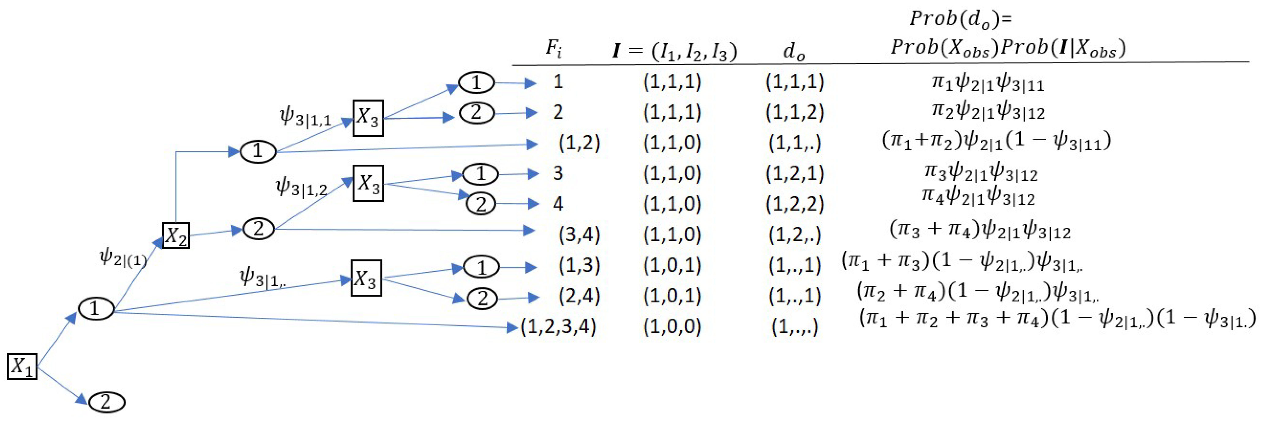
Figure 1 illustrates the notation in the $2\times 2\times 2$ case. If $x_1=1$, then the probability of collecting $x_2$ is ${\psi }_{2|x_1=1}$ or ${\psi }_{2\left|\right(1)}$ for short. If $x_2$ is collected and $x_2=1$, then the probability of collecting $x_3$ is ${\psi }_{3|x_1=1,x_2=1}$ or ${\psi }_{2\left|\right(1,1)}$. If $x_3$ is not collected, then the sample unit could either belong to cells indicated by $a=1$ (when $x_3=1$) or $a=2$ (when $x_3=2$), so the set of feasible cells is $F_i=\{1,2\}$, $d_o=\left\{(1,1,.)\right\}$ where the ‘.’ indicates the missing value of $x_3$, and the probability of the observed data from an MAR SQD is $p\left(d_o\right)=p(\mathbf{I},{\mathbf{x}}_{obs})=({\pi }_1+{\pi }_2){\psi }_{2\left|\right(1)}(1-{\psi }_{3\left|\right(1,1)})$. This $p\left(d_o\right)$ is then used in (32).

Different orderings can be considered which may lead to different efficiencies, and two or more options can be evaluated. However, there will often be practical reasons to adopt a particular ordering, for example, easy to collect and important variables can be included early in the sequence.

4. Developing MCAR and MAR PMDs

4.1. Missing Data Effects and A and D Optimality

Here we consider a standard survey of size n involving complete cases (CCs), and MCAR and MAR PMDs. For a PMD the variance matrix of $\widehat{\theta }$ is $V_M\left(\widehat{\theta }\right)=Inf{o}_M^{-1}\left(\theta \right)$, which has elements $V_M(a,b)$. For the sample comprising data for complete cases, the variance matrix is $V_{CC}\left(\widehat{\theta }\right)=Inf{o}^{-1}\left(\theta \right)$, which has elements $V_{CC}(a,b)$. For convenience we will suppress $\widehat{\theta }$. A simple way to examine the effect of a PMD on ${\widehat{\pi }}_a$ is through $V_M(a,a)/V_{CC}(a,a)$, where both variances are based on n, which we will call the Missing Data effect (MDeff(a)). This is analogous to the design effect (Deff) which measures the variance of an estimate under a complex sample design divided by the variance of the same estimate under a Simple Random Sample of the same sample size [28]. We can also define the effective sample size for the PMD as $n_a^{\ast }$ =$n/$MDeff(a). Thus, an MDeff(a) of 2 corresponds to a reduction in the effective sample size of 50 percent for ${\widehat{\pi }}_a$.

The MDeff(a) is parameter specific. An overall measure can be obtained using the concept of A-optimality, which is based on $A_M=tr{V}_M$. Define $A_{CC}=tr{V}_{CC}$. This leads to the overall missing data effect, ${MDeff}_A$=$A_M/A_{CC}$, and associated effective sample size, $n_A^{*}=n/$ ${MDeff}_A$.

Since ${MDeff}_A={\displaystyle \sum _{a=1}^{C-1}}$MDeff(a)$V_{CC}(a,a)/{\displaystyle \sum _{a=1}^{C-1}}{V}_{CC}(a,a)$, it is a weighted average of the variables’ specific MDeff(a), with weights proportional to $V_{CC}(a,a)$, which is equal to $V\left({\widehat{\pi }}_a\right)$. We can also consider giving each variable the same weight, leading to ${MDeff}_{AW}={\displaystyle \frac{1}{C-1}}{\displaystyle \sum _{a=1}^{C-1}}$MDeff(a). This is equivalent to using weights ${\pi }_a^{-1}{(1-{\pi }_a)}^{-1}$ in $A_M$, which gives $A_W$.

Corresponding measures based on D-optimality, that is the determinant of the variance matrices, $D_M=det{V}_M$ and $D_{CC}=det{V}_{CC}$, can also be used. This leads to the overall missing data effect, ${MDeff}_D$=$D_M/D_{CC}$, and associated effective sample size, $n_D^{*}=n/$ ${MDeff}_D$.

The parameter $\theta$ does not include ${\pi }_C$ because ${\pi }_C={\displaystyle \sum _{a=1}^{C-1}}{\pi }_a=1-{\mathbf{1}}^T\theta$. Then ${\widehat{\pi }}_C=1-{\mathbf{1}}^T\theta$ and $V_M\left({\widehat{\pi }}_C\right)={\mathbf{1}}^T{V}_M\left(\widehat{\theta }\right)\mathbf{1}$ and is included in global A optimality but not included in global D optimality.

These measures can be used to evaluate any specified PMD being considered. In developing a PMD the expected costs also need to be considered. For design M a simple cost function is $C_M=n_M(c_f+c_M)$ where $c_f$ is the fixed cost per sample unit, $n_M$ is the number of units selected for design M and $c_M$ is the expected cost of the variables collected per unit. In general $c_M=E_M[{\displaystyle \sum _{p=1}^P}{c}_p{I}_p]$, where $c_p$ is the cost of collecting variable p. Cost can include collection and processing costs for the survey organisation and also a quantification of the burden imposed on respondents. In the equal cost scenario, we assume $c_p=1$ so the cost of collecting each variable is the same. This will be a reasonable assumption in many surveys, but there will also be surveys where some variables are more costly to collect. Then for a standard survey in which all the variables are collected, the cost is $n_{CC}(c_f+p)$. For a survey using MCAR there are up to $2^P-1$ possible patterns and the cost is $n_{MCAR}(c_f+c_{MCAR})$, where $c_{MCAR}={\displaystyle \sum _{j=1}^{2P-1}}{p}_j{P}_j$, where $p_j$ is the probability of pattern j. For a survey using MAR, the cost is $n_{MAR}(c_f+c_{MAR})$, where $c_{MAR}={\sum }_{d_0}p\left(d_0\right)P_{d_0}$.

In some situations some variables may impose more reporting burden or collection costs than others or costs may vary in a disproportionate manner. For example, the cost of collecting a subset of variables may be more than the sum of the cost of collecting each variable.

Table 3. Variable costs scenarios.

Scenario	Cost of Variables Collected
	${\mathit{x}}_{\mathbf{1}}$	${\mathit{x}}_{\mathbf{1}},{\mathit{x}}_{\mathbf{2}}$	${\mathit{x}}_{\mathbf{1}},{\mathit{x}}_{\mathbf{3}}$	${\mathit{x}}_{\mathbf{1}},{\mathit{x}}_{\mathbf{2}},{\mathit{x}}_{\mathbf{3}}$
Equal	1	2	2	3
Unequal	1	2	4	5
Disproportionate	1	2	2	6

describes other cost scenarios. In the unequal cost scenario, the cost of collecting $x_3$ is three times the cost of collecting $x_1$ or $x_2$. The disproportionate cost scenario is the same as the equal cost scenario, except that collecting all variables together costs six times the cost of collecting a single variable.

The multinomial distribution allows for all interactions between elements of $\mathbf{x}$. Accordingly, for estimation of $\pi$ to be supported, all variables must be collected by a core sample of sufficient size to ensure the parameters are identified and the large sample ML approximation applies. Thus, we assume a core sample of size $n_{core}$ is also selected. The potential gains of a PMD are greater when the core sample is small so that its cost is small compared with the total cost. This should be balanced against identifiability considerations which suggest having at least two cases in each cell. The PMD may also involve all variables being collected from some sample units. It would be possible to not use a core sample, and in searching for optimal MCAR and MAR designs, reject those for which $Inf{o}_M\left(\theta \right)$ is non-singular. In practice having a small core sample of size $n_{core}$ will make the search for optimal designs quicker and easier. To ensure that using a core sample is not seriously affecting the efficiency, its size could be varied to assess the sensitivity of the PMD to the core sample size. An indication that the core sample is too large would be the PMD not having any complete cases.

The cost of the core sample will be added to the cost for each design, so the total sample size is $n_{core}+n_M$. To examine the cost effectiveness of a design, M, $n_M$ will be set to have the same costs as the complete case sample of size $n_{CC}$, so $n_{MCAR},n_{MAR}\ge n_{CC}$, and the use of a PMD allows a larger overall sample size for given total cost.

4.1.1. Example 1

Consider the design data in Table 2, where $P=3$ and each variable has $l_p=2$ categories. There are eight parameters for the sequential MAR PMD: two values for ${\psi }_{2|x_1}=P\left(I_2\right|x_1)$, two values for ${\psi }_{3|x_1, .}=P\left(I_3\right|I_2=0,x_1)$ and four values for ${\psi }_{3|x_1,x_2}=P\left(I_3\right|I_2=1,x_1,x_2)$. These are illustrated in Figure 1. There are four patterns of missing data under the sequential pattern given by $j=1,3,6,7$ in Table 1. To make a fair comparison, an MCAR PMD is restricted to these same four patterns and has the design parameter $p_j$, which is the proportion of the sample assigned to pattern j. In our example we set $n_{core}=715$, the sample size in Table 2, which meets the criterion of having at least two cases in each cell, and $n_{CC}$ = 10,000, so the total cost when $c_f=0$ is 32,145.

The optimal design parameters, $p_j$, for MCAR and ${\psi }_{.|.}$s for MAR, were found by a grid search, which is feasible when the number of design parameters is small. A large number of parameters can arise when there are more dimensions (i.e., $P>$ 3) or the number of levels, $l_p$, is large. In this situation more efficient algorithms, such as stochastic optimization, need to be considered.

Table 4. Percentage reduction in A-, $A_W$- and D-optimality for MCAR and sequential MAR PMDs relative to CC design for same total cost, data in Table 2, for fixed and variable cost scenarios given in Table 3.

Fixed Cost	Variable Cost	MCAR PMD			MAR PMD
$\left({\mathit{c}}_{\mathit{f}}\right)$		$\mathit{A}$	${\mathit{A}}_{\mathit{W}}$	$\mathit{D}$	$\mathit{A}$	$\mathit{AW}$	$\mathit{D}$
0	Equal	0	0	0	1.0	2.3	42
1	Equal	0	0	0	0	0	0
2	Equal	0	0	0	0	0	0
0	Unequal	0	0	0	8.5	13	92
1	Unequal	0	0	0	5.0	6.2	59
2	Unequal	0	0	0	3.7	3.1	44
0	Disproportionate	3.5	1.3	12	8.5	13	92
1	Disproportionate	0.9	0	0	5.0	6.2	59
2	Disproportionate	0	0	0	3.7	3.1	44

gives the reduction in A-, $A_W$- and D-optimality for optimal MAR and sequential MCAR designs relative to a CC design for the same total cost. Zero reduction occurs when the optimal PMD corresponds to the standard complete case design. The results show that MCAR is marginally more efficient than a CC design when costs are disproportionate (e.g., 3.5% for A optimality when $c_f=0$) but is not more efficient than CC when costs are equal or unequal. In contrast, the MAR design is significantly more efficient (up to 92% reduction ) than a CC design for D optimality and still more efficient for A- and $A_W$-optimality when costs are unequal or disproportionate. This is because when costs vary considerably, there is more cost reduction possible when not collecting the variables that are more costly to collect. The greater reductions obtained when considering D-optimality suggest that results depend on the criteria used to evaluate the PMD. In practice several criteria can be examined.

Table 5. Optimal sequential MAR PMD for A-, $A_W$- and D-optimality, same total cost: total sample size, non-core sample proportions (e.g., ${\tilde{p}}_{12}$), conditional probabilities (e.g.,${\psi }_{2|2}$), for data in Table 2, $c_f=0$, disproportionate costs given in Table 3.

Fixed	Design	Sample	Proportions	Design Parameters
Cost	Criteria	Size ($\mathit{n}$)	${\tilde{\mathit{p}}}_{\mathit{1}},{\tilde{\mathit{p}}}_{\mathit{12}},{\tilde{\mathit{p}}}_{\mathit{13}},{\tilde{\mathit{p}}}_{\mathit{123}}$	${\mathit{\psi }}_{\mathit{2}|\mathit{1}}$	${\mathit{\psi }}_{\mathit{2}|\mathit{2}}$	${\mathit{\psi }}_{\mathit{3}|\mathit{1}}$	${\mathit{\psi }}_{\mathit{3}|\mathit{2}}$	${\mathit{\psi }}_{\mathit{3}|\mathit{11}}$	${\mathit{\psi }}_{\mathit{3}|\mathit{12}}$	${\mathit{\psi }}_{\mathit{3}|\mathit{21}}$	${\mathit{\psi }}_{\mathit{3}|\mathit{22}}$
0	A	13,522	0, 0.38, 0.01, 0.61	0.6	1	1	0	0.6	1	0.8	0.4
1	A	11,207	0, 0.18, 0, 0.82	0.8	1	0	0.8	1	1	1	0.6
2	A	11,040	0, 0.18, 0.01, 0.81	0.8	1	1	0	0.8	1	1	0.6
0	$A_W$	19,061	0.39, 0.23, 0, 0.38	1	0.6	0	0	1	1	0.6	0.6
1	$A_W$	12,824	0, 0.38, 0, 0.62	1	1	0	0	1	1	0.6	0.6
2	$A_W$	12,873	0, 0.39, 0, 0.61	1	1	0	0	1	1	0.6	0.6
0	D	31,449	0.77, 0.06, 0, 0.17	1	0.2	0	0	1	1	0.6	0.8
1	D	18,995	0.38, 0.35, 0, 0.27	1	0.6	0	0	1	1	0.4	0.4
2	D	14,627	0.19, 0.39, 0, 0.42	1	0.8	0	0	1	1	0.4	0.6

Note: complete case non-core sample size = 10,000.

shows how the optimal PMD designs change according to $c_f$ and the optimality criteria when costs are disproportionate. The case of $c_f=0$ reflects cases when the reporting and collection costs are much greater, or of more concern, than the cost of the initial contact. PMDs allow for an increase in sample size, which is how the reduction in variance compared with the standard survey can arise. D optimality leads to the highest sample sizes (over 30,000 when $c_f=0$). As $c_f$ increases the total sample size approaches 10,000, the sample size for CC, since less of the cost is associated with collecting each variable. Let ${\tilde{p}}_1$, ${\tilde{p}}_{12}$, ${\tilde{p}}_{13}$ and ${\tilde{p}}_{123}$ be the proportion of units where only $x_1$, $(x_1,x_2)$, $(x_1,x_3)$ and $(x_1,x_2,x_3)$ are collected, respectively. Then ${\tilde{p}}_1+{\tilde{p}}_{12}+{\tilde{p}}_{13}+{\tilde{p}}_{123}=1$. We see that D-optimality leads to designs where a proportion of the sample collects only $x_1$, whereas A-optimality never leads to such designs, and $A_W$ optimality only once. The fact that ${\psi }_{2|1}={\psi }_{3|12}={\psi }_{3|11}=1$ for PMDs using D- and $A_W$-optimality means all variables are collected when $x_1=1$. This is because $Prob(x_1=1)$ is small and any missing data when $x_1=1$ leads to high information loss. Other common features of the PMDs are: ${\psi }_{3|1.}={\psi }_{3|2.}=0$, which means collecting $x_3$ without $x_2$ is not worthwhile, regardless of the value of $x_1$; and ${\psi }_{3|21}={\psi }_{3|22}$, which means collecting $x_3$ does not depend on the value of $x_2$ if $x_1=2$.

A-, $A_W$- and D-optimality are overall measures. The effect of a PMD can also be examined for the individual parameters by comparing the ratio of variance under the optimal design with that of a CC design of the same cost, which are the diagonal elements of the variance matrices used for Table 4.

Table 6. Ratio of variances of estimates of the parameters: optimal sequential MAR PMD relative to CC design with same total cost, for A-, $A_W$- and D-optimality, data in Table 2, disproportionate costs, $c_f=0$.

Parameter	Design Criteria
${\mathit{\pi }}_{\mathit{a}}$	$\mathit{A}$	${\mathit{A}}_{\mathit{W}}$	$\mathit{D}$
1	1.4	0.54	0.33
2	0.84	0.54	0.33
3	0.97	0.54	0.33
4	1.2	0.54	0.33
5	0.87	1.3	2.10
6	0.87	1.2	2.1
7	0.88	0.93	1.5
8	1.7	1.4	1.9

gives results for the optimal design for a sequential MAR PMD, with $c_f=0$ and disproportionate costs for these different overall criteria. We see that for D optimality the PMD reduced the variance of ${\widehat{\pi }}_j$ for $j=1,2,3,4$ to a third of that of a CC design at the cost of increasing the variance of the other parameters, particularly for $j=4,5$.

Table 7. MAR PMD, MDeff for parameters by optimal design criteria, for data in Table 2, disproportionate costs, $c_f=0$.

Parameter	Design Criteria
${\mathit{\pi }}_{\mathit{a}}$	$\mathit{A}$	${\mathit{A}}_{\mathit{W}}$	$\mathit{D}$
1	1.9	1	1
2	1.1	1	1
3	1.3	1	1
4	1.6	1	1
5	1.2	2.3	6.4
6	1.2	2.3	6.2
7	1.2	1.7	4.6
8	2.3	2.6	5.5

gives the MDeff(a) for PMDs when $c_f=0$ and variable costs are disproportionate. MDeff(a) measures the impact of missing data on the variance of parameter estimates at the design stage. The MDeff can be obtained from the preceding tables by multiplying by $(n_{core}+n_M)/(n_{core}+n_{CC})$. It shows the PMD for A-optimality loses efficiency in all parameter estimates due to the missing data. For example, the variance of ${\widehat{\pi }}_8$ is 2.3 times larger than a CC design with the same sample size, n. In contrast, for the PMDs for $A_W$- and D-optimality, the variance of ${\widehat{\pi }}_1$ to ${\widehat{\pi }}_4$ is the same as that for CC with the same sample size. As mentioned earlier, this is because all variables are collected when $x_1=1$ and so there is no loss in efficiency when estimating the four corresponding multinomial parameters.

MAR PMDs that are developed based on the overall criteria may have detrimental effects on the parameter estimates for individual cells, for example, low probability cells, if the variables defining those cells are missing more frequently, although the reverse can also occur with the PMD leading to those cells being missing less frequently. This suggests that the effects on individual parameters can be examined, as in Table 6 and Table 7.

4.1.2. Example 2

We repeated the process using A-optimality and D-optimality for the marginal means (i.e., proportions): $y_1=\delta (x_1=1)$, $y_2=\delta (x_2=1)$ and $y_3=\delta (x_3=1)$ with corresponding mean parameters ${\mu }_1=1-{\pi }_5-{\pi }_6-{\pi }_7-{\pi }_8$, ${\mu }_2={\pi }_3+{\pi }_4+{\pi }_7+{\pi }_8$, and ${\mu }_3={\pi }_2+{\pi }_4+{\pi }_6+{\pi }_8$, respectively. If $\widehat{\mu }=({\widehat{\mu }}_1,{\widehat{\mu }}_2,{\widehat{\mu }}_3)$, $Va{r}_M\left(\widehat{\mu }\right)$ has $(k,k^{\prime })$ element $Co{v}_M({\widehat{\mu }}_k,{\widehat{\mu }}_{k^{\prime }})={\mathbf{c}}_k^{T}V\left(\widehat{\theta }\right){\mathbf{c}}_{k^{\prime }}$, where ${\mathbf{c}}_k$ depends on the expression for ${\mu }_k$ in terms of the $\pi$ parameters (e.g., ${\mathbf{c}}_1=(0,0,0,-1,-1,-1,-1)$.

Table 8. Means: percentage reduction in A-, $A_W$- and D-optimality for MCAR and sequential MAR PMDs relative to CC design for same total cost, data in Table 2, for fixed and variable cost scenarios given in Table 3.

Fixed Cost	Variable Cost	MCAR			MAR
$\left({\mathit{c}}_{\mathit{f}}\right)$		$\mathit{A}$	$\mathit{AW}$	$\mathit{D}$	$\mathit{A}$	$\mathit{AW}$	$\mathit{D}$
0	Equal	0	0	0	2.3	3.2	7.8
1	Equal	0	0	0	0.8	1.7	2.3
2	Equal	0	0	0	0	0.8	1.0
0	Unequal	7.4	13	35	11	15	41
1	Unequal	2.8	6.8	15	6.4	9.3	21
2	Unequal	1.1	3.6	5.4	4.0	6.4	13
0	Disproportionate	11	19	50	15	22	55
1	Disproportionate	6.0	10	28	9.8	14	36
2	Disproportionate	2.8	6.8	15	6.7	9.7	22

presents the reduction in variance for the mean estimates for the MAR and MCAR optimal designs using the A-, $A_W$- and D-optimality criteria compared to a sample of CCs with the same total cost. The results show that MCAR designs are more efficient than the CC design when costs are unequal or disproportionate, with the strongest gains for D-optimal design. The MAR designs are more efficient than the MCAR designs. As before, gains are greater when $c_f$ is smaller.

The results show that MAR designs can dramatically reduce the variance for some parameter estimates while increasing it for others. There are trade-offs that may need to be considered, especially if the survey objectives prioritize specific parameters. As part of the design, the importance of different parameters needs to be identified and the parameter specific evaluations considered as in Table 6 and Table 7, as well as the overall criteria. In some cases the importance of a specific parameter can be incorporated into the criteria, for example, importance weight in $A_W$-optimality.

To develop a PMD some assumptions have to be made on the values of the cell probabilities, $\pi$. This is a general issue affecting the development of any survey design—the efficiency of a possible design will depend on the values of some unknown population parameters. Practice values are obtained from previous or related surveys, pilot data or administrative data. It is useful to check the sensitivity of the design to misspecification of the underlying multinomial probabilities used at the design stage by varying the parameters. For a contingency table there may be data available on the marginal distribution of the variables. These can be combined with data or assumptions on interactions, including that some may be zero, to produce likely values of the cell probabilities.

4.2. Marginal Effects of Missing Data for a Single Unit

At the sample design stage, there are advantages in having an analytic expression for the marginal effect or influence that a particular value for $d_{o,i}$ has on the optimality of an MAR PMD. (It may be worthwhile incorporating cost into the assessment of the marginal effect, but we do not here for simplicity.) First, this could be incorporated into criteria for splitting a questionnaire, as in the data-driven approach in [7], that avoids having to recalculate the information matrix for each possible split. Second, it can be used to constrain elements of $\psi$ so that undesirable values of $d_{o,i}$ either do not occur or occur with a low probability. This simplifies the design and reduces the computation required to find the optimum. Below we consider how to assess this impact and illustrate the approach using data in Table 2.

Take the situation where a large sample of size n is taken of complete cases. Consider the option of instead collecting $d_{oi}$ from a single unit and incurring a loss of information given by $l(\theta ;d_{oi})$. We can apply (32) where we have set $p\left(d_{o,i}\right)=1$ for the unit, and for all other units complete data are obtained. Then

$$Inf{o}_M\left(\theta \right)=Info\left(\theta \right)-\mathbf{l}(\theta ;d_{oi})$$

let ${\mathbf{l}}_i=\mathbf{l}(\theta ;d_{oi})$. Taking the inverse of $Inf{o}_M\left(\theta \right)$ gives

$$\begin{array}{cc}{V}_M\hfill & =V_{CC}{[\mathbf{I}-V_{CC}{\mathbf{l}}_i]}^{-1}\hfill \\ \hfill & \approx V_{CC}[\mathbf{I}+V_{CC}{\mathbf{l}}_i]\hfill \\ \hfill & =V_{CC}+\Delta \hfill \end{array}$$

(33)

Here $\mathit{I}$ is the identity matrix and we have used the approximation ${[\mathit{I}-\mathit{B}]}^{-1}\approx \mathit{I}+\mathit{B}$ when $\mathit{B}$ is small and set $\Delta =V_{CC}{V}_{CC}{\mathbf{l}}_i.$ The i subscript is dropped for convenience.

Consider the effect on $tr{V}_M$. Define ${\varphi }_A=ntr\Delta /tr{V}_{CC}$; then ${MDeff}_A=1+{\varphi }_A/n$ and the effective sample size $n_A^{\ast }=n{(1+{\varphi }_A/n)}^{-1}.$ It is useful to consider the reduction in effective sample size, which is $n-n_A^{\ast }={\varphi }_A{(1+{\varphi }_A/n)}^{-1}\approx {\varphi }_A$ when n is large. When the data are independently and identically distributed, $V_{CC}=V_1/n$ and ${\varphi }_A=tr\left[V_1{\mathbf{l}}_i{V}_1\right]/tr{V}_1.$ In the multinomial case

$$\begin{array}{cc}{V}_1(a,b)\hfill & ={\pi }_a(1-{\pi }_a) if a=b\hfill \\ \hfill & =-{\pi }_a{\pi }_b if a \ne b\hfill \end{array}$$

(34)

For $det{V}_M$ we use the approximation $det[\mathit{I}+\mathit{B}]\approx 1+tr\mathit{B}$; then similar results apply with ${\varphi }_A$ replaced by ${\varphi }_D=ntr\left[V_{CC}{\mathbf{l}}_i\right]=tr\left[V_1{\mathbf{l}}_i\right].$

For the parameter ${\pi }_a$, using (33) gives similar results with ${\varphi }_A$ replaced by ${\varphi }_A\left(a\right)=n\Delta (a,a)/V_{CC}(a,a)=n^2\Delta (a,a)/V_1(a,a)={\Delta }_1(a,a)/V_1(a,a)$, where ${\Delta }_1=V_1{V}_1{l}_i$. Similarly, for D-optimality we could replace ${\varphi }_D$ with ${\varphi }_D\left(a\right)$, the $(a,a)$th element of $V_1{\mathbf{l}}_i$.

Table 9. Reduction in the effective sample size for the possible data observed on a single unit, data in Table 2, for each parameter, $\varphi \left(a\right)$, and for overall A- and D-optimality, $\varphi$.

${\mathit{x}}_1$	${\mathit{x}}_2$	${\mathit{x}}_3$	$\mathit{\varphi }\left(2\right)$	$\mathit{\varphi }\left(3\right)$	$\mathit{\varphi }\left(4\right)$	$\mathit{\varphi }\left(5\right)$	$\mathit{\varphi }\left(6\right)$	$\mathit{\varphi }\left(7\right)$	$\mathit{\varphi }\left(8\right)$	$\mathit{\varphi }$
Observed Values MAR			A-optimality
1	.	.	27.50	27.50	27.50	−0.61	−0.63	−0.77	−0.47	0.62
1	1	.	35.75	−0.73	−0.72	−0.96	−1.0	−1.2	−0.75	0.18
1	.	1	−0.33	102	−0.33	−0.43	−0.45	−0.55	−0.34	0.35
1	2	.	0	40	80	0	0	0	0	0.64
1	.	2	3.97	0	34	0	0	0	0	0.27
2	.	.	0	0	0	1.1	1.1	0.85	1.3	0.97
2	1	.	0	0	0	1.4	1.2	0	0	0.72
2	.	1	0	0	0	1.1	1.1	0.85	1.3	0.97
2	2	.	0	0	0	0	0	0.17	3.0	0.19
2	.	2	0	0	0	0	0.35	0	3.7	0.27
Observed Variables MCAR
✓			1.0	1.0	1.0	1.1	1.0	0.79	1.3	0.73
✓	✓		1.00	0.31	0.65	0.69	0.60	0.04	1.3	0.47
✓		✓	0.10	1.0	0.90	0.73	0.81	0.55	2.0	0.69
✓	✓	✓	0	0	0	0	0	0	0
Observed Values MAR			D-optimality
1	.	.	28	28	28	0	0	0	0	83
1	1	.	38	0	0	0	0	0	0	38
1	.	1	0	102	0	0	0	0	0	102
1	2	.	0	39	79	0	0	0	0	119
1	.	2	4.0	0	34	0	0	0	0	38
2	.	.	0	0	0	0.77	0.74	0.60	1.0	3.1
2	1	.	0	0	0	1.0	0.90	0	0	1.9
2	.	1	0	0	0	0.8	0.7	0.6	1.0	3.1
2	2	.	0	0	0	0	0	0.2	2.10	2.3
2	.	2	0	0	0	0	0	0	2.9	3.2
Observed Variables MCAR
✓			1.0	1.0	1.0	0.74	0.71	0.57	0.96	5.0
✓	✓		1.0	0.31	0.66	0.52	0.47	0.07	0.92	4.0
✓		✓	0.10	1.0	0.89	0.50	0.59	0.40	1.55	6.0
✓	✓	✓	0	0	0	0	0	0	0	0

shows how the reduction in effective sample size depends on the observed values in $d_{oi}$, for example, 1. It gives ${\varphi }_A$ and ${\varphi }_D$, as well as ${\varphi }_A\left(a\right)$ and ${\varphi }_D\left(a\right)$ for $a=2,\dots ,8$ for all possible values of $d_{oi}$. Because what is missing depends on the observed variables and the values they take, these results correspond to MAR. The table shows the reduction in the effective sample size depends greatly on the observed data. For both A and D optimality, the reduction in the effective sample size for ${\pi }_3$ when we observe only $x_1=1$ and $x_3=1$ on a unit is equivalent to dropping the CC sample size by 102, and when we observe only $x_1=1$, the reduction is 28 for ${\pi }_2$, ${\pi }_3$ and ${\pi }_4$. When the reduction in the effective sample size is significantly greater than 1, ${\varphi }_A\left(a\right)\approx {\varphi }_D\left(a\right)$, meaning there is little difference whether the A and D optimality criteria are used. However, when the reduction in effective sample is close to 1, differences between ${\varphi }_A\left(a\right)$ and ${\varphi }_D\left(a\right)$ emerge. For example, for the observed data $x_1=2$, ${\varphi }_A\left(8\right)=1.3$ and ${\varphi }_D\left(8\right)=1.0$.

By definition, the reduction in the effective sample must be non-negative when data are missing for a unit. However, when $x_1=1$, some ${\varphi }_A\left(a\right)$ values are negative. This occurs because $l_i$ is not positive definite and, because its elements can be much larger than $V_1^{-1}$, $V_1{V}_i{\mathbf{l}}_i$ has negative diagonal elements. The value of $x_1=1$ is an influential data point because it is 26 times less likely than $x_1=2$, and is the reason the approximation used to derive ${\varphi }_A\left(a\right)$ leads to negative values. This is an artefact of the approximation affecting the trace criterion for specific parameters associated with relatively rare variables and suggests the need for improved approximations in such cases. The negative values of ${\varphi }_A\left(a\right)$ for A optimality are replaced by 0s in the corresponding values for D-optimality, ${\varphi }_D\left(a\right)$.

Another interesting feature of Table 9 is the number of zeros, indicating no difference between collecting the observed and complete data on the accuracy of a parameter. The pattern of 0s reflects, for instance, if we observe $x_1=1$, there is no additional benefit to estimating ${\pi }_5$ to ${\pi }_8$ by further collecting $x_2$ or $x_3$.

Table 9 also shows the expected reduction in effective sample size depending on what variables are observed. These results do not depend on the values of the variables and take the expectation of the loss for all possible values of the observed variables and correspond to MCAR. The values for MAR are much more variable than MCAR, which are between 0 and 2.0 for A optimality. This highlights the fact that knowing the values of observed variables, not just the pattern of observed variables, is more useful in measuring the impact of missing data on the accuracy of estimates.

5. Discussion

A PMD enables a reduction in the reporting load for respondents and also a reduction in data collection costs. For a PMD that uses an MCAR or MAR approach, MLEs can be obtained once the data have been collected using the observed likelihood and resulting score function. This ensures all the data collected are effectively used and correspond to full information maximum likelihood. The Missing Information Principle can be used to obtain the observed score function from the complete data score function and also the observed information function. It clearly shows the information lost due to the variables that are missing compared to estimation based on complete cases. A PMD can be more efficient than a standard survey collecting all variables in some situations since the reduction in reporting and collection costs enables a larger total sample to be used for the same total cost.

At the design stage no data have been collected, and to develop a PMD we need to consider the expected information and associated information loss. With few exceptions, previous works on PMDs have only allowed the data to be MCAR. This paper gives a framework for designing a PMD that allows the data to be MAR, so that the pattern of variables for which data are collected depends on the values of some of the variables. We focussed on a simple MAR PMD, called a sequential PMD, but there are many other options to be considered. A feature of MAR PMDs is there flexibility and adaptivity as decisions on which variables to collect depend on the observed values of some key variables. This also improves robustness as it can be used to ensure particular combinations of variables are collected from an adequate number of units.

For many surveys the key outputs consist of contingency tables. We derive the observed and expected score and information for a multinomial model for the cell frequencies. The expected information can be used to evaluate the likely variances for any specified PMD being considered. They are then used to develop and evaluate possible MCAR and MAR designs using A- and D-optimality. The effect on the variance of the estimates of cell probabilities and the marginal probabilities are also considered. We also develop ways of assessing the marginal effect of reducing the variables collected from a single sample unit.

A number of criteria to develop and evaluate potential PMDs have been considered here. A-optimality is very easy to understand and is proportional to the average of the variance of the parameter estimates. It is easily modified by applying weights to the variances of the parameter estimate to reflect their relative importance. D-optimality minimizes the volume of the confidence ellipsoid for the parameter estimates and is a good overall measure of efficiency. In some cases, particular criteria or parameters may be of interest, but in many surveys a range of outputs are to be produced. In practice we would look at several criteria to help guide us on a sensible design.

It would be useful to have mathematically precise sufficient conditions to ensure identifiability of the multinomial parameters. We see this as a topic for further research. Identifiability will occur when the expected information matrix is non-singular. Because we are focusing on the design of a PMD, different choices of the size of the core sample can be tried and the resulting expected information matrix checked to see if it is non-singular.

In an empirical evaluation, we show that an MAR PMD can be more efficient than an optimal MCAR PMD or standard survey which collects all the variables, particularly when the costs for each variable are unequal or vary in a disproportionate way. When costs for each variable are equal, the PMDs may not be any more efficient than a standard survey. The evaluation focuses on estimating parameters of the multinomial model, which allows for all interactions between variables. A PMD can lose considerable information about interactions. Further work into designing an MAR PMD can consider tables for which higher order interactions are not of interest or other target parameters, including parameters in various analytical models (e.g., loglinear, linear and logistic regression).

Developing more effective algorithms to identify efficient PMDs is a major challenge for future research. The fundamental theory on information loss developed in this paper provides the basis for such development. Using the unit level information loss considered in Section 4.2 could be useful in developing more efficient search algorithms. If some interactions are not of interest or are zero, then that will reduce the number of parameters and the size of the search space.

As in all modelling the model and parameterisation need to be considered. This will involve structural considerations and interpretability, as well as robustness to model and parameter misspecification. We focus on a reasonably general survey producing key tables. We have not made any structural assumptions and allowed for all interactions to be present. It may be possible to assume some specific structure in some situations corresponding to some higher order interaction being absent. Considering how the efficiency of PMDs changes as higher order interactions are set to zero can be part of robustness considerations. The robustness of the PMDs to uncertainty associated with parameters values assumed at the design stage can also be examined.

This paper provides the general theory for developing MCAR and MAR PMDs based on the expected information. It considers the reasonably general case of the multinomial distribution for a contingency table, providing explicit formulas for the information, and information loss, which can be used to developed MCAR and MAR PMDs. There are a number of issues such as sensitivity to model assumptions and challenges in specifying realistic MAR mechanisms at the design stage that need further consideration. The general approach can be used to consider extensions beyond the multinomial model, such as generalized linear models or models for continuous outcomes. Ref. [3] considers multivariate normal and Ref. [8] considers logistic regression with binary covariates. An issue for analyses involving models for an outcome variable given a set of covariates is that to use the MIP it is necessary to use a model for the joint distribution of the outcome variable and the covariates, even though only the conditional distribution is of interest.

References

1. Chambers, R.L.; Steel, D.G.; Wang, S.; Welsh, A. Maximum Likelihood Estimation for Sample Surveys; CRC Press Taylor and Francis Group: Boca Raton, FL, USA, 2012. [Google Scholar]
2. Kim, J.; Shao, J. Statistical Methods for Handling Incomplete Data; CRC Press: Boca Raton, FL, USA, 2021. [Google Scholar]
3. Chipperfield, J.O.; Steel, D.G. Efficiency of Split Questionnaire Surveys. J. Stat. Plan. Inference 2012, 141, 1925–1933. [Google Scholar] [CrossRef] [Scilit]
4. Chipperfield, J.O.; Steel, D.G. Design and Estimation for Split Questionnaire Surveys. J. Off. Stat. 2009, 25, 227–244. [Google Scholar]
5. Schoemann, A.M.; Miller, P.; Pornprasertmanit, S.; Wu, W. Using Monte Carlo simulations to determine power and sample size for planned missing designs. Int. J. Behav. Dev. 2014, 38, 471–479. [Google Scholar] [CrossRef] [Scilit]
6. Jang, D.G.; Zhu, Z.; Yu, C. A-Optimal Split Questionnaire Designs for Multivariate Continuous Variables. arXiv 2022, arXiv:2203.04883. [Google Scholar] [CrossRef] [Scilit]
7. Adiguzel, F.; Wedel, M. Split Questionnaire Designs for Massive Surveys. J. Mark. Res. 2008, 45, 608–617. [Google Scholar] [CrossRef] [Scilit]
8. Chipperfield, J.O.; Barr, M.L.; Steel, D.G. Split Questionnaire Designs: Collecting only the data that you need through MCAR and MAR designs. J. Appl. Stat. 2018, 45, 1465–1475. [Google Scholar] [CrossRef] [Scilit]
9. Lin, C.; Peng, J.; Qin, Y.; Li, Y.; Yang, Y. Optimal Integrating Learning for Split Questionnaire Design Type Data. J. Comput. Graph. Stat. 2022, 32, 1009–1023. [Google Scholar] [CrossRef] [Scilit]
10. Raghunathan, T.E.; Grizzle, J.E. A split questionnaire survey design. J. Am. Stat. Assoc. 1995, 90, 54–63. [Google Scholar] [CrossRef]
11. Axenfeld, J.B.; Blom, A.G.; Bruch, C.; Wolf, C. Split Questionnaire Designs for Online Surveys: The Impact of Module Construction on Imputation Quality. J. Surv. Stat. Methodol. 2022, 10, 1236–1262. [Google Scholar] [CrossRef] [Scilit]
12. Lang, K.M.; Moore, E.W.G.; Grandfield, E.M. A novel item-allocatioran procedure for the three-form planned missing data design. MethodsX 2020, 7, 100941. [Google Scholar] [CrossRef] [Scilit] [PubMed]
13. Wu, W.; Jia, F.; Rhemtulla, M.; Little, T.D. Search for efficient complete and planned missing data designs for analysis of change. Behav. Res. Methods 2016, 48, 1047–1061. [Google Scholar] [CrossRef] [Scilit] [PubMed]
14. Stuart, M.; Yu, C. A computationally efficient method for selecting a split questionnaire design. Commun. Stat.-Simul. Comput. 2022, 51, 2464–2486. [Google Scholar] [CrossRef] [Scilit]
15. Lyberg, L.; Biemer, P.; Collins, M.; de Leeuw, E.; Dippo, C.; Schwarz, N.; Trewin, D. Survey Measurement and Process Quality; John Wiley and Sons: Hoboken, NJ, USA, 1997. [Google Scholar]
16. Rubin, D.B.; Little, R.J.A. Statistical Analysis of Missing Data; John Wiley and Sons: Hoboken, NJ, USA, 1987. [Google Scholar]
17. Enders, C.K. Applied Missing Data Analysis; Guilford Press: New York, NY, USA, 2022. [Google Scholar]
18. Silvia, P.J.; Kwapil, T.R.; Walsh, M.A.; Myin-Germeys, I. Planned missing-data designs in experience-sampling research: Monte Carlo simulations of efficient designs for assessing within-person constructs. Behav. Res. Methods 2014, 46, 41–54. [Google Scholar] [CrossRef] [Scilit]
19. Lawes, M.; Schultze, M.; Eid, M. Making the Most of Your Research Budget: Efficiency of a Three-Method Measurement Design with Planned Missing Data. Assessment 2020, 27, 903–920. [Google Scholar] [CrossRef] [Scilit]
20. Noble, D.W.A.; Nakagawa, S. Planned missing data designs and methods: Options for strengthening inference, increasing research efficiency and improving animal welfare in ecological and evolutionary research. Evol. Appl. 2021, 14, 1958–1968. [Google Scholar] [CrossRef] [Scilit] [PubMed]
21. Imbriano, P.M.; Raghunathan, T.E. Three-Form Split Questionnaire Design for Panel Surveys. J. Off. Stat. 2020, 36, 827–854. [Google Scholar] [CrossRef] [Scilit]
22. Ioannidis, E.; Merkouris, T.; Zhang, L.C.; Karlberg, M.; Petrakos, M.; Reis, F.; Stavropoulos, P. On a Modular Approach to the Design of Integrated Social Surveys. J. Off. Stat. 2016, 32, 259–286. [Google Scholar] [CrossRef] [Scilit]
23. Rioux., C.; Lewin, A.; Odejimi, O.A.; Little, T.D. Reflection on modern methods: Planned missing data designs for epidemiological research. Int. Stat. Rev. 2020, 49, 1702–1711. [Google Scholar] [CrossRef] [Scilit] [PubMed]
24. Rhemtulla, M.; Hancock, G.R. Planned Missing Data Designs in Educational Psychology Research. Educ. Psychol. 2016, 51, 305–316. [Google Scholar] [CrossRef] [Scilit]
25. Gonzalez, J.M.; Eltinge, J.L. Multiple Matrix Sampling: A Review; Office of Survey Methods Research: Washington, DC, USA, 2007. [Google Scholar]
26. Orchard, T.; Woodbury, M.A. A missing information principle: Theory and applications. In Proceedings of the 6th Berkeley Symposium on Mathematical Statistics and Probability; University of California Press: Berkeley, CA, USA, 1972; Volume 1, pp. 697–715. [Google Scholar]
27. Agresti, J. An Introduction to Categorical Data Analysis; John Wiley and Sons: Maitland, FL, USA, 1996. [Google Scholar]
28. Kish, L. Survey Sampling; John Wiley & Sons: Hoboken, NJ, USA, 1965. [Google Scholar]
Figure 1. Monotonic sequential MAR SQD with three categorical variables: ψ is the conditional probability of observing the indicated sequence; F i give feasible cells for the observed sequence; I indicates the variables observed; d o is the values of observed variables; p ( d 0 ) is the probability of d 0 .
Mathematics 14 00355 g001