Weighted, Mixed ℓ_p Norm Regularization for Gaussian Noise-Based Denoising Method Extension

Abstract

Many denoising methods model noise as Gaussian noise. However, the realistic noise captured by camera devices does not satisfy Gaussian distribution. Hence, those methods do not perform well when being applied to real-world image denoising tasks. In this work, we indicate that the spatial correlation in noise and the variation of noise intensity are the main factors that impact the performance of Gaussian noise-based methods, and accordingly propose an extension of the method based on the weighted, mixed non-convex ${\mathsf{\ell }}_p$ norm. The proposed method first strengthens the intensity of the noise pattern in the original denoising result through the Guided Filter, then removes the over-amplified frequency in the local area by the proposed regularization term. We prove that the optimal solution can be achieved through the sub-gradient-based iterative optimization scheme, and further reduce the computational cost by optimizing the initial values. Numerical experiments show that the proposed extending method can balance well texture preservation and noise removal, and the PSNR of the extending method’s results are greatly improved, even outperforming the recently proposed realistic noise removal methods which also include deep learning based methods.

1. Introduction

Image denoising is an important research field in image processing. The image acquired by digital devices is often corrupted due to various reasons, such as quantization noise and poor illumination conditions [1]. Because the Gaussian noise is the distribution with the highest entropy under fixed variance, this means it can better analogize noise that is generated from multiple aspects. Many denoising methods simplify the noise as additive white Gaussian noise (AWGN) [2,3].

However, the distribution of realistic noise is much more complicated. After acquiring the raw image from sensor, the camera devices adopt complex Image Signal Processor (ISP) nonlinear operations such as demosaicing, white balance, color correction, denoising, etc., to achieve the desired image quality. Because the demosaicing process [4] adopts an interpolation scheme to estimate the missing pixel values, this means the noise distribution loses its independence and the pattern of noise exhibits more complex spatial correlations [5], especially in low frequencies [5] after demosaicing. Additionally, due to the fact that the amount of light trapped by a single pixel is lower in low-light conditions and higher when over-exposed, the noise does not always satisfy the zero mean and its intensity relates to the lighting conditions. Therefore, realistic noise is usually spatially correlated in low frequency [6], and its intensity is not invariant across the whole image [7], which means the distribution of noise at different positions is no longer independent and may greatly differ. Hence, there is a significant gap between realistic noise and synthetic noise, which satisfies i.i.d in an entire image [8], and the Gaussian noise-based methods do not work well on realistic noise removal since they can not effectively remove spatially correlated noise and there are strong artifacts in denoising results.

Although the denoising methods for Gaussian noise and realistic noise have huge differences in noise modelling, their assumptions on noise-free natural images are the same—for example, non-local self similarity (NSS) [9], low complexity in most areas [10,11], and clear and continuous boundaries [12,13]. Non-local similarity refers to the fact that in natural images, a local patch often has many similar patches within its neighbour area, and has been widely utilized in patch-based image restoration methods, such as denoising [2], dehazing [14] and demosaicing [15]. Low complexity means the image is very smooth and nearly flat in most areas, and only a small part of the image contains texture and edge information, which further indicates that the gradient of image is near zero in most parts [16]. Clear and continuous boundaries imply that the boundary in natural images is sharp and clear, and usually remains continuous in a wide area. Combined with the low complexity assumption, some researchers point out that the gradient of natural images is heavy-tailed and has a non-Gaussian distribution [17].

To address the problem that realistic noise is spatially correlated and varies in different positions and scenarios, and to make full use of Gaussian-based methods, we try to suppress the remaining noise in denoising results from the Gaussian noise-based method. Because the artifacts in denoising results are mainly the remaining low-frequency part of the realistic image, using the noisy image as the guidance to perform the Guided Filter on denoising results will amplify the intensity of the artifacts. The factor of amplification in the local area relates to the noise intensity and complexity of original image. We prove that if the low-frequency part of noise is not well removed, the flat area would have a higher amplification factor than in the texture area. Hence, the artifacts in denoising results can be removed by suppressing the coefficients that are over-amplified in the Guided Filtering result.

Besides the ${\mathsf{\ell }}_0$ and ${\mathsf{\ell }}_1$ norms, which are commonly used as regularization terms in image denoising, the weighted norm is also widely used in many signal processing methods [18] since it can flexibly penalize the non-zero coefficients. Xiao and Liao [19] employ the weighted ${\mathsf{\ell }}_1$ norm to improve the sparse signal recovery performance in compressed sensing. Meng et al. [20] accelerate the convergence by expanding the attraction range of the zero attractor of the weighted ${\mathsf{\ell }}_0$ norm. The mixed norm is also studied by many researchers. Compared with the single norm, the mixed norm has better performance in terms of handling highly dimensional data [21], despite it often being harder to optimize than single norm. Bu et al. [22] employ a mixed norm tensor penalty to describe low-rank structures in the local area for tensor completion. In this work, we propose a weighted, mixed ${\mathsf{\ell }}_p$ norm regularizer, which is a weighted combination of two different ${\mathsf{\ell }}_p$ norms intended to suppress coefficients in the Fourier transform domain and to suppress renaming noise in denoising results from Gaussian-based methods.

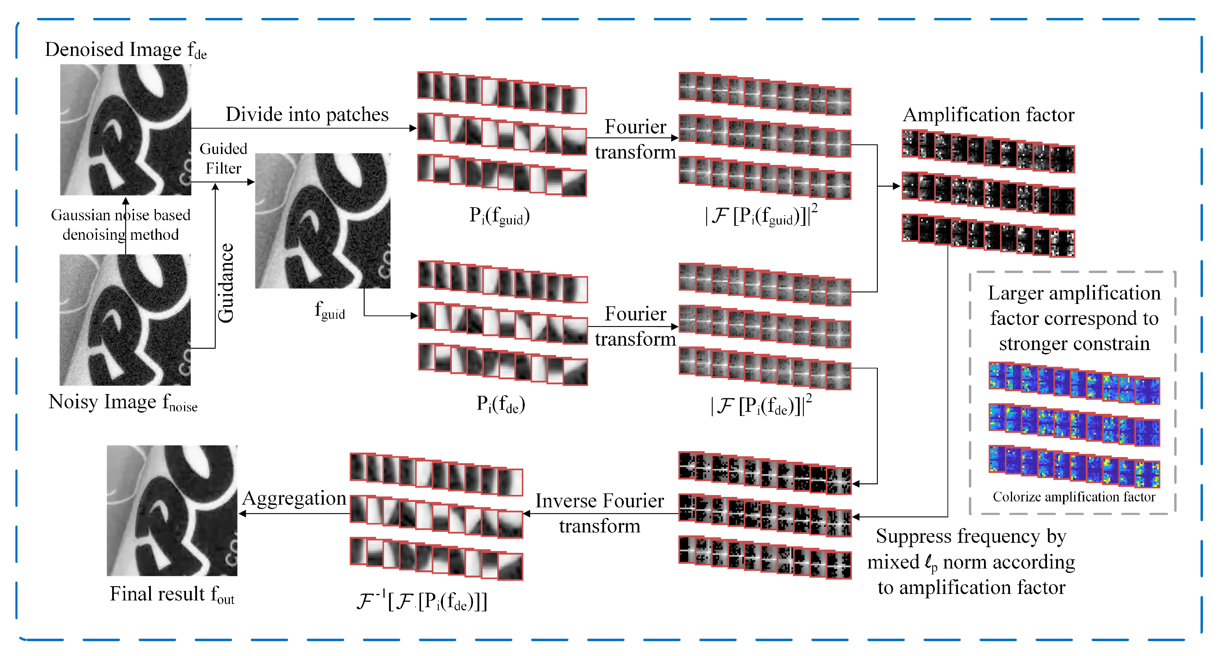
The weighting coefficients for the regularization term are based on the amplification ratio in the frequency domain. The proposed optimization problem is analysed under different cases, and we prove that it can be solved by an iterative scheme. Additionally, we design an initial value selection scheme that can reduce the distance between the initial value and optimal solution to further reduce the iteration steps. The final result is obtained by aggregating the optimized image patches. The overall extending procedure is presented in Figure 1.

Algorithm 1 Denoising process of the proposed method

Require: Noisy image $f_{\mathrm{noise}}$ and original denoised image $f_{\mathrm{de}}$ Ensure: Denoised image $f_{\mathrm{out}}$  $f_{\mathrm{guid}}=\mathrm{Guided}\mathrm{Filter}(f_{\mathrm{noise}},f_{\mathrm{de}})$  for each image patch $P_j\left(f_{\mathrm{de}}\right)$ do     for $i=1,2,\dots ,N$ do          $x_{ij}={\mathcal{F}}_i\left[P_j\left(f_{\mathrm{de}}\right)\right]$, $F_{ij}={\mathcal{F}}_i\left[P_j\left(f_{\mathrm{guid}}\right)\right]$          $s_{ij}=0$          if $|x_{ij}|>0$ and ${\tau }_p|F_{ij}{|}^2|x_{ij}{|}^p+{\tau }_q|F_{ij}\left|\right|x_{ij}{|}^q\le {\left|x_{ij}\right|}^2$ then               ${\lambda }_p=p{\tau }_p|F_{ij}{|}^2{\left|x_{ij}\right|}^{p-2}$               ${\lambda }_q=q{\tau }_q|F_{ij}{|}^2{\left|x_{ij}\right|}^{q-2}$               $s_{ij}={({\displaystyle \frac{1+{\lambda }_p(p-2)+{\lambda }_q(q-2)}{1+{\lambda }_p(p-1)+{\lambda }_q(q-1)}})}_{+}$               $t_{ij}=0$               while $\underset{ij}{max}|t_{ij}-s_{ij}|\ge$$ϵ$ do                    $t_{ij}=s_{ij}$                    $s_{ij}={(1-{\lambda }_p{t}_{ij}^{p-1}-{\lambda }_q{t}_{ij}^{q-1})}_{+}$               end while               if ${\displaystyle \frac{1}{2}}{(s_{ij}-1)}^2+{\displaystyle \frac{1}{p}}{\lambda }_p{s}_{ij}^p+{\displaystyle \frac{1}{q}}{\lambda }_q{s}_{ij}^q>{\displaystyle \frac{1}{2}}$ then                    $s_{ij}=0$               end if            end if       end for  end for  Aggregate all ${\mathcal{F}}_i^{-1}\left[s_{ij}{x}_{ij}\right]$ to obtain $f_{\mathrm{out}}$

Numerical experiments on multiple mainstream denoising datasets show that the proposed method can extend the Gaussian-based methods to realistic noise removal tasks effectively. The artifacts are eliminated and the PSNR of results is greatly improved. What is more, in the Renoir dataset [23], the proposed extending method even makes the outdated Gaussian noise-based denoising method outperform the recently proposed realist noise denoising methods, which also include deep learning based methods, which shows the extending ability of the proposed method. The mathematical notations used in this paper are listed in

Table 1. Mathematical notations.

Notation	Description
$f_{\mathrm{gt}}$	noise-free image
$f_{\mathrm{noise}}$	realistic noisy image
$f_{\mathrm{guid}}$	Guided Filtering result
$f_{\mathrm{de}}$	denoising result from the Gaussian noise-based method
$f_{\mathrm{out}}$	final denoised image
$\mathcal{F}[·]$	Fourier transform
${\mathcal{F}}_i[·]$	i-th frequency of Fourier transform
$P_i(·)$	i-th patch of image
$\mathrm{Cov}(·,·)$	Covariance
$\mathrm{Var}(·)$	Variance
$n_i$	Fourier transform of noise
$f_i$	Fourier transform of ground truth image
$x_{ij}$	i-th Fourier transform coefficients of j-th patch of $f_{\mathrm{de}}$
$F_{ij}$	i-th Fourier transform coefficients of j-th patch of $f_{\mathrm{guid}}$
$t_{ij}$	optimization variable for the proposed optimization problem
$a_{ij}$	optimization variable for the reformulated optimization problem

.

2. Related Works

The ${\mathsf{\ell }}_p$ norm-based method has been widely used in image denoising. Yin et al. [24] combine the filtered least mean square algorithm with the ${\mathsf{\ell }}_p$ norm to improve its performance under strong $\alpha$-stable noise such as impulsive noise. Korki et al. [25] propose a weighted diffusion least mean p-power algorithm and a corresponding adaptive weighted diffusion continuous mixed p-norm for distribution estimation in sensor networks under non-uniform noise. Apart from noise removal, Ma et al. [26] developed the diffusion recursive least $L_p$ norm for distributed estimation over network.

In this work, we focus on realistic noise that is spatially correlated in low-frequency parts rather than impulsive noise or Gaussian noise, which means the characteristics of noise distributions are greatly different. Additionally, the proposed method attempts to remove remaining noise from the initial denoising results that are obtained via Gaussian noise-based methods. Hence, we adopt the ${\mathsf{\ell }}_p$ norm on the regularization term instead of the data fidelity term as in [24,25].

Due to the convexity of the ${\mathsf{\ell }}_p$ norm when $0<p<1$, it has stronger constraints on smaller variables, which makes the optimization result exhibit sparsity. Su et al. [27] adopt the ${\mathsf{\ell }}_p$ norm in the regularization term and propose a multi-band weighted norm minimization algorithm for image denoising. Xu et al. [28] propose a weighted ${\mathsf{\ell }}_p$ norm sparse error constraint as the regularization term and solve it by alternating the direction method of the multipliers algorithm. Tan et al. [29] combine the weighted Schatten p-norm, lp-norm, and total variation regularization in image denoising. The weighted Schatten p-norm ensures global low rankness, while the lp-norm provides noise robustness.

Compared with the single ${\mathsf{\ell }}_p$ norm, mixed ${\mathsf{\ell }}_p$ norms can suppress variables in a more flexible way by adjusting hyper-parameters p and q. Sadraeifar et al. [30] use a mixed $L_p$–$L_q$ norm regularization in a constrained inversion process to generate compact and smooth models in three dimensions. The $L_p$ and $L_q$ norms are used to penalize the deviation of model parameters and gradients. Vatankhah et al. [31] designed an effective and general algorithm for the mixed $L_p$ norm joint inversion of gravity and magnetic datasets. Two different norms are used to measure the size of the model with respect to the initial model and the smoothness of the subsurface model along the three orthogonal directions, respectively. Song et al. [32] adopted a convex mixture of ${\mathsf{\ell }}_p$ and ${\mathsf{\ell }}_q$ norms on residual error as a loss function for active noise control under Gaussian and non-Gaussian noise environments.

In the proposed method, we use the traditional ${\mathsf{\ell }}_2$ norm in data fidelity terms and the mixed ${\mathsf{\ell }}_p$ norm in regularization terms, as in [32]. Numerical experiments show that the proposed method has better performance with the proposed mixed norm compared with the single norm.

3. Spatial Correlation in Realistic Noise

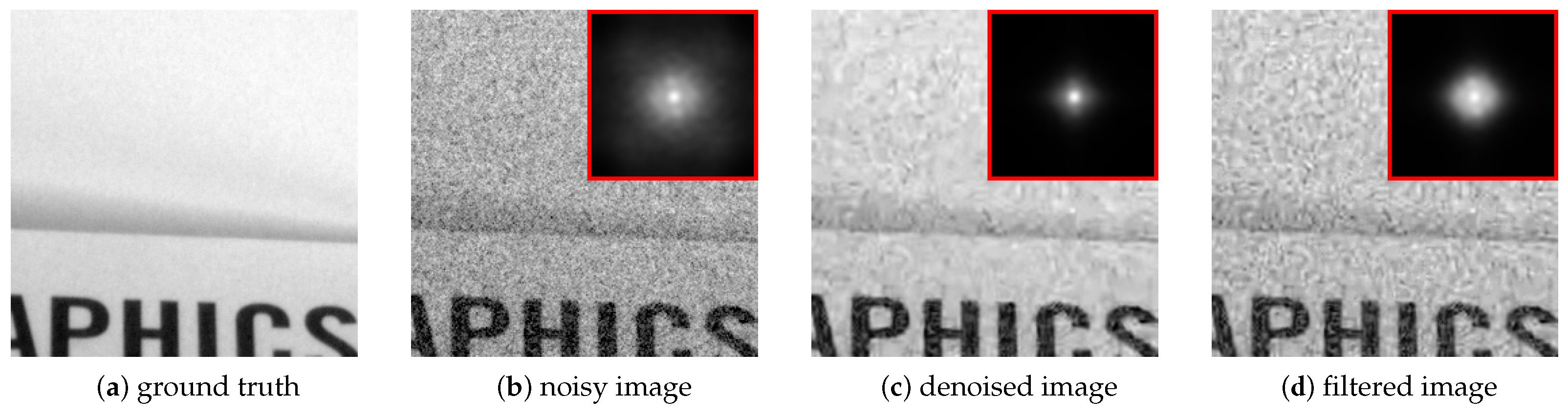
The Gaussian noise-based denoising methods fail to remove realistic noise with spatial correlation in low frequencies. As shown in Figure 2, the power spectral density (PSD) distribution of the denoised image is greatly shrunk and gathered at the central area compared with the PSD of the noisy image, which means that only the high-frequency part of noise is well removed and the denoising result still has very strong artifacts which come from the low-frequency part of noise. This is because the regularizer for Gaussian noise removal is not suitable for realistic noise.

The image denoising method can be roughly treated as using an image to fit the noisy image under a certain regularizer. There are various kinds of regularizers, such as low-rankness [33], total variation [16], ${\mathsf{\ell }}_1$ norm in the transform domain [34], and the nuclear norm [35]. Sometimes, the regularizer is also related to the noisy image itself, such as NSS prior [9]. The regularizer removes noise from noisy images by forcing the result to have a lower complexity when fitting the noisy image. Stronger regularizers will over-smooth the result, while weaker regularizers can not effectively remove the noise. Finding the balance between smoothing and fitting is the key to denoising.

Many common regularizers such as the ${\mathsf{\ell }}_1$ and ${\mathsf{\ell }}_2$ norms in the frequency domain can be considered as shrinkage methods.

$${\parallel \mathcal{F}\left[x\right]\parallel }_1=\sum _i\left|{\mathcal{F}}_i\left[x\right]\right|,{\parallel \mathcal{F}\left[x\right]\parallel }_2=\sqrt{\sum _i{\left|{\mathcal{F}}_i\left[x\right]\right|}^2}.$$

where $\mathcal{F}$ denotes the Fourier transform and ${\mathcal{F}}_i$ denotes its i-th component. What is more, the nuclear norm and total variation regularizer can also be treated as shrinkage in the frequency domain. Since the singular value of the matrix under Fourier transformation is invariant, this means the singular value of A and $\mathcal{F}\left[A\right]$ are the same and ${\parallel A\parallel }_{*}={\parallel \mathcal{F}\left[A\right]\parallel }_{*}$. Total variation is defined on the spatial domain, and because of the linearity of Fourier transformation, it also satisfies convexity in the frequency domain.

For non-spatially correlated noise like $n_{\mathrm{gauss}}$, it is easy to prove that both the expectation and the variance of energy in each frequency are invariant. Due to the energy of the image being mainly distributed at lower frequencies [36] in most natural images, the PSD of the noise and original image are only slightly overlapped, and the smoothness-based denoising methods can effectively remove Gaussian noise. However, the correlation in realistic noise $n_{\mathrm{real}}$ causes the energy distribution to be much more concentrated than in Gaussian noise [37], which makes the noise smoother than Gaussian noise and its PSD highly overlapped with original image. Hence, the lower frequencies of noisy images are much stronger. Due to the fact that frequency with a larger absolute value displays stronger shrinkage under most regularizers, the lower frequencies of denoising results are more variable and may be far from the ground truth, which causes those regularizers for Gaussian noise removal to fail to remove realistic noise.

4. Proposed Methods

In this section, first we indicate that the Guided Filter can amplify the remaining noise in denoising results and analyse the amplification ratio in different areas, and then we introduce the proposed weighted, mixed ${\mathsf{\ell }}_p$ norm-based extending method and its optimization scheme.

4.1. Noise Amplification

We denote the original noise-free image as $f_{\mathrm{gt}}$, the additive noise corrupted image as $f_{\mathrm{noise}}=f_{\mathrm{gt}}+n_{\mathrm{real}}$, and the corresponding denoising result as $f_{\mathrm{de}}$. The result of the Guided Filter [38] on $f_{\mathrm{noise}}$, with $f_{\mathrm{de}}$ as the guidance image, is denoted as $f_{\mathrm{guid}}$. The coefficients of the Guided Filter in the local area without Box Filter are as follows:

$$k_{\mathrm{guid}}={\displaystyle \frac{\mathrm{Cov}(f_{\mathrm{noise}},f_{\mathrm{de}})}{\mathrm{Var}\left(f_{\mathrm{de}}\right)}},b_{\mathrm{guid}}=\mathrm{Mean}\left(f_{\mathrm{noise}}\right)-\mathrm{Mean}\left(f_{\mathrm{de}}\right)·k_{\mathrm{guid}},$$

(1)

where $\mathrm{Cov}(·,·)$ denotes the covariance and $\mathrm{Var}(·)$ denotes the variance.

In the local area, we use $\left\{f_i\right\}$ and $\left\{n_i\right\}$ to denote the Fourier transform of the noise-free image and the noise, and $\left\{p_i\right\}$ and $\left\{q_i\right\}$ to denote the expectation of the shrink ratio of $f_i$ and $n_i$ in $f_{\mathrm{de}}$ over noise $n_{\mathrm{real}}$ respectively:

$$p_i={\mathcal{F}}_i[{\displaystyle \frac{f_{\mathrm{de}}}{f_{\mathrm{gt}}}}],q_i={\mathcal{F}}_i[{\displaystyle \frac{f_{\mathrm{de}}-E\left(f_{\mathrm{de}}\right)}{n_{\mathrm{real}}}}].$$

(2)

Because the denoising methods usually cause blurriness in the denoising results, especially at the edges [13], and because, as analysed in the last section, the shrinkage coefficients $p_j$ and $q_j$ both decrease as the frequency grows in each direction, we assume $0\le p_i,q_i\le 1$.

Because the covariance between two discrete signals is equal to the inner product of their Fourier series, we start from second term. We rewrite $k_{\mathrm{guid}}$ in summation of the Fourier series, as follows:

$$k_{\mathrm{guid}}={\displaystyle \frac{{\sum }_2^N(p_i{f}_i^2+q_i{n}_i^2+(p_i+q_i)f_i{n}_i)}{{\sum }_2^N(p_i^2{f}_i^2+q_i^2{n}_i^2+2p_i{q}_i{f}_i{n}_i)}},$$

(3)

where ${\sum }_2^N$ denotes the sum from second term and N is the number of pixels in filtering range. Next, we analyse $k_{\mathrm{guid}}$ in the smooth area and texture area separately.

In the smooth area, the intensity of noise $n_{\mathrm{real}}$ is much higher than $f_{\mathrm{gt}}$. If we assume ${\sum }_2^N|f_i{|}^2\le {\mu }_1{\sum }_2^N{\left|n_i\right|}^2$, then we obtain the following:

$$\begin{array}{cc}\hfill k_{\mathrm{guid}}& \ge {\displaystyle \frac{{\sum }_2^N(q_i{n}_i^2-(p_i+q_i)|f_i\left|\right|n_i\left|\right)}{{\sum }_2^N(q_i^2{n}_i^2+{\mu }_1{n}_i^2+2p_i{q}_i|f_i\left|\right|n_i\left|\right)}}\hfill \\ \hfill & \ge {\displaystyle \frac{{\sum }_2^N(q_i{n}_i^2-2|f_i\left|\right|n_i\left|\right)}{{\sum }_2^N(q_i^2{n}_i^2+{\mu }_1{n}_i^2+2|f_i\left|\right|n_i\left|\right)}}\ge {\displaystyle \frac{{\sum }_2^N(q_i{n}_i^2-2{\mu }_1{n}_i^2)}{{\sum }_2^N(q_i^2{n}_i^2+3{\mu }_1{n}_i^2)}}.\hfill \end{array}$$

(4)

Hence, when ${\mu }_1$ is only slightly higher than zero,

$$k_{\mathrm{guid}}\approx {\displaystyle \frac{{\sum }_2^N\left(q_i{n}_i^2\right)}{{\sum }_2^N\left(q_i^2{n}_i^2\right)}}.$$

(5)

We can see that the ratio of amplification is proportional to the reciprocal of the shrink rate $q_i$, which means that if $n_{\mathrm{real}}$ is not well removed, the noise in the Guided Filtering result will be amplified almost to its original intensity in $n_{\mathrm{noise}}$.

In the texture area, $f_{\mathrm{gt}}$ is at the dominant position. Because we assume noise $n_{\mathrm{real}}$ is additive and not related to $f_{\mathrm{gt}}$, it therefore is reasonable to assume the correlation coefficient $\tau$ between zero averaged $n_{\mathrm{real}}$ and $f_{\mathrm{gt}}$ is close to zero:

$${\mu }_2={\displaystyle \frac{\mathrm{Cov}(f_{\mathrm{gt}},n_{\mathrm{real}})}{\sqrt{\mathrm{Var}\left(f_{\mathrm{gt}}\right)·\mathrm{Var}\left(n_{\mathrm{gauss}}\right)}}}={\displaystyle \frac{{\sum }_2^N{f}_i{n}_i}{\sqrt{\left({\sum }_2^N{f}_i^2\right)\left({\sum }_2^N{n}_i^2\right)}}}\approx 0.$$

(6)

Then we have the following:

$$k_{\mathrm{guid}}\le {\displaystyle \frac{{\sum }_2^N(p_i{f}_i^2+q_i{n}_i^2)+2\left|{\mu }_2\right|\sqrt{\left({\sum }_2^N{f}_i^2\right)\left({\sum }_2^N{n}_i^2\right)}}{{\sum }_2^N(p_i^2{f}_i^2+q_i^2{n}_i^2)-2\left|{\mu }_2\right|\sqrt{\left({\sum }_2^N{f}_i^2\right)\left({\sum }_2^N{n}_i^2\right)}}}\approx {\displaystyle \frac{{\sum }_2^N(p_i{f}_i^2+q_i{n}_i^2)}{{\sum }_2^N(p_i^2{f}_i^2+q_i^2{n}_i^2)}}.$$

(7)

Because in the texture area, the image details are stronger and better preserved than noise, this means the following:

$${\displaystyle \frac{{\sum }_2^N{p}_i{f}_i^2}{{\sum }_2^N{p}_i^2{f}_i^2}}<{\displaystyle \frac{{\sum }_2^N{q}_i{n}_i^2}{{\sum }_2^N{q}_i^2{n}_i^2}},$$

(8)

Therefore we obtain

$$k_{\mathrm{guid}}<{\displaystyle \frac{{\sum }_2^N{q}_i{n}_i^2}{{\sum }_2^N{q}_i^2{n}_i^2}}.$$

(9)

Based on the analysis above, we can conclude that $k_{\mathrm{guid}}$ in the texture area is smaller than in the smooth area, which means that the noise in smooth area is expected to have a larger amplification rate. As shown in Figure 2, the distribution of the PSD of $f_{\mathrm{guid}}$ is flatter than that of $f_{\mathrm{de}}$ and more centralized than that of $f_{\mathrm{noise}}$. Therefore, by suppressing the frequency of $f_{\mathrm{de}}$ that significantly grows in $f_{\mathrm{guid}}$ in the local area, the low-frequency, spatial, correlated noise $n_{low}$ can be suppressed. Because the analysis is discussed in the local area of the image, we divide the image into overlapping patches, remove noise in each of them, and then aggregate to obtain the final denoising result.

4.2. Weighted ${\mathsf{\ell }}_p$ Norm

As analysed in last subsection, the remaining noise in $f_{\mathrm{de}}$ can be depressed by removing the amplified coefficients in $f_{\mathrm{guid}}$. We adopt the weighted, mixed ${\mathsf{\ell }}_p$ norm as the regularizer and propose the following optimization problem:

$$\begin{array}{cc}\hfill \underset{t_{ij}}{min}& \sum _{ij}({\displaystyle \frac{1}{2}}{(t_{ij}-x_{ij})}^2+{\tau }_p|F_{ij}{|}^2|t_{ij}{|}^p+{\tau }_q|F_{ij}\left|\right|t_{ij}{|}^q),\hfill \\ \hfill s.t.& 0\le t_{ij}{x}_{ij}\le x_{ij}^2,\forall i,j\hfill \end{array}$$

(10)

where ${\tau }_p,{\tau }_q>0$, $0<p,q<1$, $t_{ij}$ denotes the optimization variable, and $x_{ij}$ and $F_{ij}$ represent the i-th Fourier transform coefficient in j-th patch in $f_{\mathrm{de}}$ and $f_{\mathrm{guid}}$, respectively. Obviously, the proposed optimization problem does not satisfy convexity. To simplify the optimization, we reformulate the optimization problem as follows:

$$\begin{array}{cc}\hfill \underset{a_{ij}}{min}& \sum _{ij}|x_{ij}{|}^2({\displaystyle \frac{1}{2}}{(a_{ij}-1)}^2+{\tau }_p|F_{ij}{|}^2|x_{ij}{|}^{p-2}{a}_{ij}^p+{\tau }_q|F_{ij}\left|\right|x_{ij}{|}^{q-2}{a}_{ij}^q),\hfill \\ \hfill s.t.& 0\le a_{ij}\le 1,\forall i,j,\hfill \end{array}$$

(11)

where $a_{ij}$ denotes the optimization variable. The optimal solution of above optimization problem is denoted as $a_{ij}^{*}$; we can see that the solution of Equation (10) is $t_{ij}^{*}=a_{ij}^{*}{x}_{ij}$, and the optimization problem is transformed from finding the optimal complex number $x_{ij}$ to the real number $a_{ij}$.

Next, we discuss the optimal solution and convergence of the proposed optimization problem. Let

$$\Phi \left(t\right)={\displaystyle \frac{1}{2}}{(t-x)}^2+{\lambda }_p{t}^p+{\lambda }_q{t}^q,t>0,$$

(12)

where $x>0$ and ${\lambda }_p,{\lambda }_q>0$, and its derivative is

$$\varphi \left(t\right)={\displaystyle \frac{𝜕\Phi \left(t\right)}{𝜕t}}=t-x+p{\lambda }_p{t}^{p-1}+q{\lambda }_q{t}^{q-1}.$$

(13)

Because ${\lambda }_p,{\lambda }_q>0$, the minimum point of $\Phi \left(t\right)$ in $[0,+\infty )$ is obviously located in $[0,x)$. The derivative of $\varphi \left(t\right)$ is as follows:

$${\varphi }^{\prime }\left(t\right)={\displaystyle \frac{𝜕\varphi \left(t\right)}{𝜕t}}=1-p(1-p){\lambda }_p{t}^{p-2}-q(1-q){\lambda }_q{t}^{q-2}.$$

(14)

Because $0<p,q<1$, both $t^{p-2}$ and $t^{q-2}$ decrease in $(0,\infty )$ and tend to negative infinity as t approaches zero and as t tends to infinity. Therefore, ${\varphi }^{\prime }\left(t\right))$ tends to negative infinity as t approaches zero and tends to one as t approaches infinity, which means that ${\varphi }^{\prime }\left(t\right)$ has one sign-changing zero point $\widehat{t}$ at most when $t\in [0,x]$; that is, $\varphi \left(t\right)$ decreases from infinity first and then increases to infinity if ${\varphi }^{\prime }\left(x\right)>0$. If ${\varphi }^{\prime }\left(x\right)\le 0$, $\varphi \left(t\right)$ will keep decreasing in $[0,x]$. Because $\varphi \left(x\right)=p{\lambda }_p{x}^{p-1}+q{\lambda }_q{x}^{q-1}>0$, $\varphi \left(t\right)>0$ in $[0,x]$, this means $L\left(t\right)$ keeps increasing in $[0,x]$ and the minimum point is zero.

Next, we discuss the minimum point of $\Phi \left(t\right)$ when ${\varphi }^{\prime }\left(x\right)>0$, which means ${\varphi }^{\prime }\left(t\right)$ has sign-changing zero point $\widehat{t}$, under different situations based on the value of $\varphi \left(\widehat{t}\right)$.

1. $\varphi \left(\widehat{t}\right)<0$. $\varphi \left(t\right)$ has two sign-changing zero points $t_a$ and $t_b$, and satisfies $t_a<\widehat{t}<t_b$. Hence, $\Phi \left(t\right)$ is increasing in $[0,t_a)\cup [t_b,\infty )$ and decreasing in $[t_a,t_b)$, and the minimum point of $\Phi \left(t\right)$ is either $t_b$ or zero.

2. $\varphi \left(\widehat{t}\right)>0$. $\Phi \left(t\right)$ is increasing in $[0,\infty )$ and the minimum point is obtained at zero.

3. $\varphi \left(\widehat{t}\right)=0$. $\Phi \left(t\right)$ is the same as in the second situation, except that $\varphi \left(t\right)$ has a critical point in $\widehat{t}$.

To obtain the minimum point in the first situation, we propose the sub-gradient-based [39] iterative scheme [40], as follows:

$$t_{n+1}=\left\{\begin{array}{cc}\psi {\left(t_n\right)}_{+}={(x-p{\lambda }_p{t}_n^{p-1}-q{\lambda }_q{t}_n^{q-1})}_{+},\hfill & t_n>0,\hfill \\ 0,\hfill & t_n\le 0,\hfill \end{array}\right.$$

(15)

and discuss its convergence under three different situations respectively.

1. We can see that $\psi \left(t\right)=t-\varphi \left(t\right)$; hence, ${\psi }^{\prime }\left(t\right)=1-{\varphi }^{\prime }\left(t\right)$. As analysed above, $0<{\varphi }^{\prime }\left(t\right)<1$ in $(\widehat{t},+\infty )$; then, $\forall t_0>t_b$ and $c_1$ and $c_2$ satisfy $0<c_1<{\varphi }^{\prime }\left(t\right)<c_2<1$ in $[t_b,t_0]$, and we have $0<1-c_2<{\psi }^{\prime }\left(t\right)<1-c_1<1$ in $[t_b,t_0]$. Because $\psi \left(t_b\right)=t_b-\varphi \left(t_b\right)=t_b>0$ and $\psi \left(t\right)>0$ in $[t_b,\infty )$, $\psi \left(t\right)$ is a contraction mapping in $[t_b,t_0]$.

$$\begin{array}{cc}\hfill t_{n+1}-t_b& =\psi \left(t_n\right)-t_b=\psi \left(t_n\right)-\psi \left(t_b\right)-t_b={\psi }^{\prime }\left(\xi \right)(t_n-t_b)-t_b\hfill \\ \hfill & <(1-c_1)(t_n-t_b)-t_b<(1-c_1)(t_n-t_b),\hfill \end{array}$$

(16)

where $\xi \in [t_b,t_n]$. Therefore, $t_n$ will converge to $t_b$ under the iterative scheme Equation (15) when the initial value $t_0>t_b$.

If the initial value $t_0\in (t_a,t_b-ϵ]$, $\forall 0<ϵ<t_b-\widehat{t}$, then due to $\varphi \left(t\right)<0$, when $t\in (t_a,t_b)$ and $\varphi \left(t\right)$ we only have two zero points $t_a$, $t_b$, and there exists ${ϵ}_0<0$ which satisfies $\varphi \left(t\right)<{ϵ}_0$ when $t\in (t_0,t_b-ϵ]$; then we have the following:

$$t_{n+1}-t_n=\psi \left(t_n\right)-t_n=t_n-\varphi \left(t_n\right)-t_n=-\varphi \left(t_n\right)>-{ϵ}_0>0,$$

(17)

which means $t_n$ is increased with respect to n and is able to grow bigger than $t_b-ϵ$ in finite steps. Due to ${\psi }^{\prime }\left(t\right)=1-{\varphi }^{\prime }\left(t\right)>0$, when $t\in (t_a,t_b)$ and there are only two points, $t_a$ and $t_b$, that satisfy $\psi \left(t\right)=t$, and we have $t_a<\psi \left(t\right)<t_b$ when $t\in (t_a,t_b)$. Hence, $t_n$ can not grow bigger than $t_b$. Because $0<{\varphi }^{\prime }\left(t\right)<1$, when $t>\widehat{t}$, there exists c, which satisfies $c<1-{\varphi }^{\prime }\left(t\right)<1$ when $t\in [t-{ϵ}_0,t_b]$, and we have the following:

$$\begin{array}{cc}\hfill t_{n+1}-t_b& =\psi \left(t_n\right)-t_b=t_n-\varphi \left(t_n\right)-t_b\hfill \\ \hfill & =-(\varphi \left(t_n\right)-\varphi \left(t_b\right))+t_n-t_b=-{\varphi }^{\prime }\left(\xi \right)(t_n-t_b)+t_n-t_b\hfill \\ \hfill & =(1-{\varphi }^{\prime }\left(\xi \right))(t_n-t_b)<c(t_n-t_b)\hfill \end{array}$$

(18)

where $\xi \in (t_n,t_b)$. Hence, $\psi \left(t\right)$ is a contraction mapping in $[t-{ϵ}_0,t_b)$. Therefore, $t_n$ will also converge to $t_b$ under iterative scheme Equation (15) when initial value $t_0\in (t_a,t_b)$.

If $t_0\in (0,t_a)$, there exists $\widehat{c}$, which satisfies $\varphi \left(\widehat{t}\right)>\widehat{c}>0$, and we have the following:

$$t_{n+1}-t_n=-\varphi \left(t_n\right)<-\widehat{c}<0.$$

(19)

Hence, $t_n$ is decreased as n increases when $t_0\in (0,t_a)$, and $t_n$ will converge to zero in finite steps.

From the analysis above, we can conclude that $t_n$ converge to $t_b$ when the initial value $t_0>t_a$ and zero when $t_0<t_a$. Additionally, $t_n=t_a$$\forall n$ when $t_0=t_a$, Based on the similar analysis in first situation, we can obtain the convergence in other two situations:

2. $t_n$ converges to zero in finite steps under the iterative scheme Equation (15) when $t_0\ge 0$.

3. $t_n$ converges to $\widehat{t}$ when $t_0\ge \widehat{t}$ and zero when $t_0<\widehat{t}$.

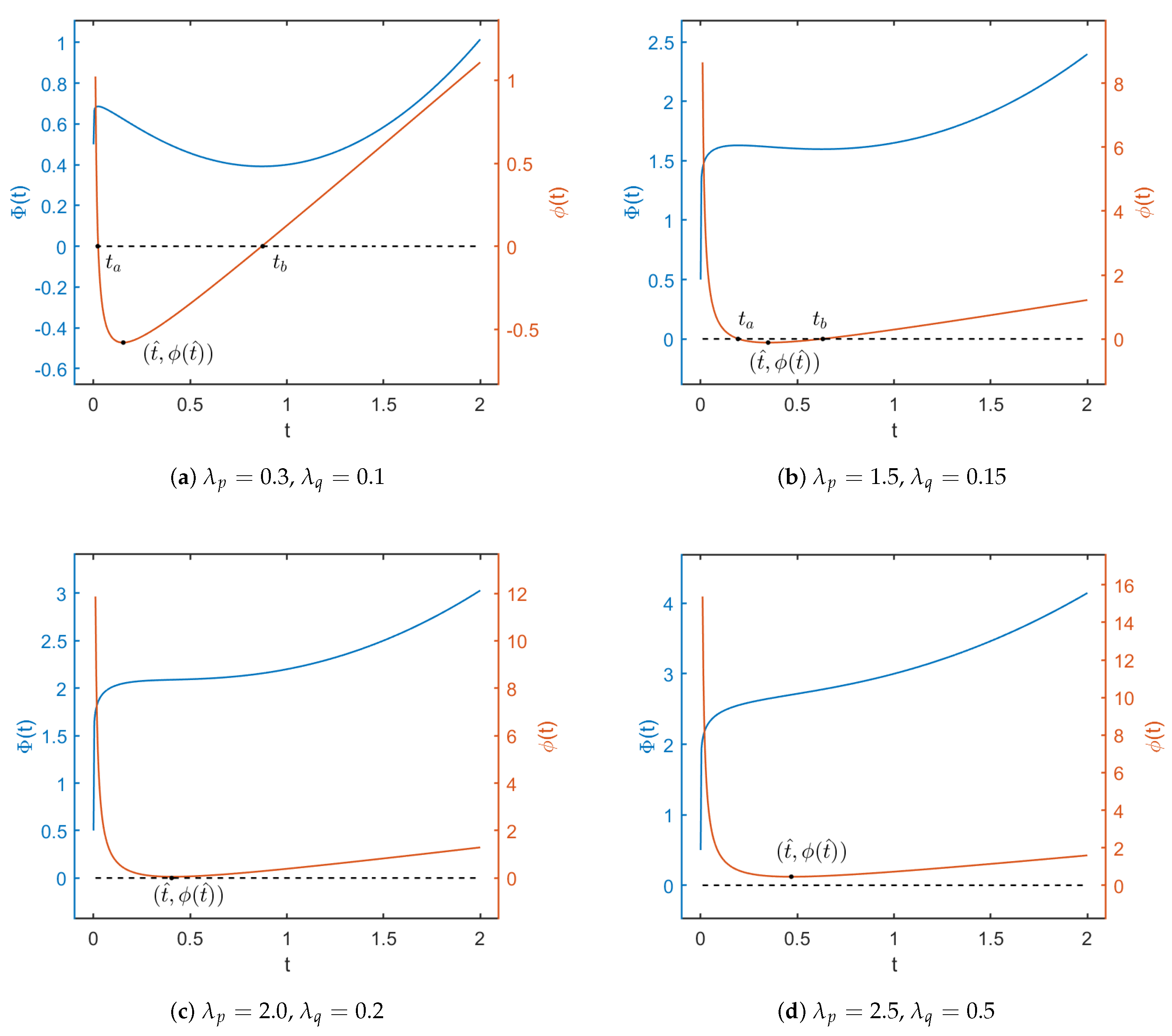
However, in first situation, $\Phi \left(t_b\right)$ does not guarantee to have the lowest value, and we still need to compare $\Phi \left(t_b\right)$ and $\Phi \left(0\right)$ to determine id the minimum point is $t_b$ or zero. Figure 3 illustrates the loss function and its derivatives under different situations.

5. Initial Value Selection

The proposed iterative scheme is able to converge under the initial value $t_0=x$. We can adopt the solution from a weaker regularizer, which can be solved explicitly as the initial value to further reduce the computation. The following optimization problem substitutes the original regularization term by a quadratic function:

$$\begin{array}{cc}\hfill \underset{a_{ij}}{min}& \sum _{ij}|x_{ij}{|}^2({\displaystyle \frac{1}{2}}{(a_{ij}-1)}^2+{\tau }_p|F_{ij}{|}^2{|x_{ij}|}^{p-2}({\displaystyle \frac{p(p-1)}{2}}{a}_{ij}^2+(2p-p^2)a_{ij})\hfill \\ \hfill & +{\tau }_q|F_{ij}\left|\right|x_{ij}{|}^{q-2}({\displaystyle \frac{q(q-1)}{2}}{a}_{ij}^2+(2q-q^2)a_{ij})),\hfill \\ \hfill s.t.& 0\le a_{ij}\le 1,\forall i,j.\hfill \end{array}$$

(20)

Its solution ${\tilde{a}}_{ij}^{*}$ can be expressed explicitly as follows:

$${\tilde{a}}_{ij}^{*}=\left\{\begin{array}{cc}{({\displaystyle \frac{1+{\tau }_p|F_{ij}{|}^2|x_{ij}{|}^{p-2}(p^2-2p)+{\tau }_q|F_{ij}\left|\right|x_{ij}{|}^{q-2}(q^2-2q)}{1+{\tau }_p|F_{ij}{|}^2|x_{ij}{|}^{p-2}(p^2-p)+{\tau }_q|F_{ij}\left|\right|x_{ij}{|}^{q-2}(q^2-q)}})}_{+}\hfill & |x_{ij}|>0\hfill \\ 0\hfill & |x_{ij}|=0.\hfill \end{array}\right.$$

(21)

To ensure the convexity of the loss function in the above optimization problem, we assume the coefficient of second order term as $1+|F_{ij}{|}^2|x_{ij}{|}^{p-2}p(p-1)+|F_{ij}{|}^2{\left|x_{ij}\right|}^{q-2}q(q-1)\ge 0$, which holds in the numerical experiments in this work. Next, we prove that ${\displaystyle \frac{p(p-1)}{2}}{a}_{ij}^2+(2p-p^2)a_{ij}$ is a weaker regularizer compared with $a_{ij}^p$ when $0\le a_{ij}\le 1$, and ${\tilde{a}}_{ij}^{*}$ satisfies $a_{ij}^{*}\le {\tilde{a}}_{ij}^{*}\le 1$, which means ${\tilde{a}}_{ij}^{*}$ is a better initial value compared with one in Equation (11).

Let $t=a_{ij}$, ${\lambda }_p={\tau }_p|F_{ij}{|}^2{\left|x_{ij}\right|}^{p-2}$, and ${\lambda }_q={\tau }_q|F_{ij}\left|\right|x_{ij}{|}^{q-2}$; then, the loss function of $a_{ij}$ under two different regularization term can be expressed as follows:

$$\begin{array}{cc}\hfill L_1\left(t\right)& ={\displaystyle \frac{1}{2}}{(t-1)}^2+{\lambda }_p{t}^p+{\lambda }_q{t}^q,\hfill \\ \hfill L_2\left(t\right)& ={\displaystyle \frac{1}{2}}{(t-1)}^2+p{\lambda }_p({\displaystyle \frac{p-1}{2}}{t}^2+(2-p)t)+q{\lambda }_q({\displaystyle \frac{q-1}{2}}{t}^2+(2-q)t),\hfill \end{array}$$

(22)

where ${\lambda }_p,{\lambda }_q>0$, $0<p,q<1$, and $0\le t\le 1$. The minimum point of $L_1\left(t\right)$ and $L_2\left(t\right)$ are denoted as $t_1^{*}$ and $t_2^{*}$ respectively. The derivatives of $L_1\left(t\right)$ and $L_2\left(t\right)$ are as follows:

$$\begin{array}{cc}\hfill {\varphi }_1\left(t\right)& ={\displaystyle \frac{𝜕L_1\left(t\right)}{𝜕t}}=t-1+p{\lambda }_p{t}^{p-1}+q{\lambda }_q{t}^{q-1},\hfill \\ \hfill {\varphi }_2\left(t\right)& ={\displaystyle \frac{𝜕L_2\left(t\right)}{𝜕t}}=t-1+p{\lambda }_p((p-1)t+2-p)+q{\lambda }_q((q-1)t+2q-q^2).\hfill \end{array}$$

(23)

Because $t^{p-1}$ is a convex function, $\zeta \left(t\right)=t^{p-1}-((p-1)t+2p-p^2)$ is also a convex function, and its derivative is

$${\displaystyle \frac{𝜕\zeta \left(t\right)}{𝜕t}}=(p-1)t^{p-2}-(p-1).$$

(24)

We can see that its minimum point is obtained at $t=1$ where the derivative is 0, and $\zeta \left(t\right)\ge \zeta \left(1\right)=0$ when $0<t<1$. Therefore, when $t_1^{*}>0$,

$${\varphi }_2\left(t_1^{*}\right)={\varphi }_1\left(t_1^{*}\right)-\zeta \left(t_1^{*}\right)<0.$$

(25)

Since $L_2\left(t\right)$ is a convex function, its second-order derivative $1+p{\lambda }_p(p-1)+q{\lambda }_q(q-1)>0$, according to the assumption, ${\varphi }_2\left(t\right)$, has only one sign-changing zero point at most, and the minimum point $t_2^{*}$ of $L_2\left(t\right)$ satisfies ${\varphi }_2\left(t_2^{*}\right)=0$, which means that $t_1^{*}\le t_2^{*}$ and proves that $|a_{ij}^{*}|\le |{\tilde{a}}_{ij}^{*}|$.

What is more, if the minimum point of $L_1\left(t\right)$ in Equation (22) satisfies $0<t_1^{*}<1$, we obtain the following:

$$\begin{array}{cc}\hfill & {\displaystyle \frac{1}{2}}{(t_1^{*}-1)}^2+{\lambda }_p{\left(t_1^{*}\right)}^p+{\lambda }_q{\left(t_1^{*}\right)}^q<{\displaystyle \frac{1}{2}}\iff {\displaystyle \frac{t_1^{*}}{2}}+{\lambda }_p{\left(t_1^{*}\right)}^{p-1}+{\lambda }_q{\left(t_1^{*}\right)}^{q-1}<1\hfill \\ \hfill \Rightarrow & {\lambda }_p{\left(t_1^{*}\right)}^{p-1}+{\lambda }_q{\left(t_1^{*}\right)}^{q-1}<1.\hfill \end{array}$$

(26)

Because ${\left(t_1^{*}\right)}^{p-1},{\left(t_1^{*}\right)}^{q-1}>1$, we can obtain the following:

$${\lambda }_p+{\lambda }_q={\tau }_p|F_{ij}{|}^2|x_{ij}{|}^{p-2}+{\tau }_q|F_{ij}\left|\right|x_{ij}{|}^{q-2}<1.$$

(27)

Therefore, if ${\tau }_p|F_{ij}{|}^2|x_{ij}{|}^p+{\tau }_q|F_{ij}\left|\right|x_{ij}{|}^q>{|x_{ij}|}^2$, the minimum point $t_{ij}^{*}=0$.

The overall optimization scheme with better initial values for Equation (10) are presented in Algorithm 1, where $P_j(·)$ denotes the j-th patch of an image.

6. Numerical Experiments

The numerical experiments are conducted on several mainstream realistic denoising datasets: the SIDD [41] dataset, Renoir [23] dataset, and PolyU dataset. Due to the limitation of computational resources, the experiments are only performed on the central $256\times 256$ square area of the green channel of each image. The patch size of the proposed method is $16\times 16$ and the stride of patch is four in both directions; the hyper-parameters of the mixed ${\mathsf{\ell }}_p$ norm are $p=0.002$, $q=0.96$, ${\tau }_p=0.29$, and ${\tau }_q=0.02$, and the convergence criterion $ϵ=0.001$.

6.1. Introduction of Denoising Methods and Datasets

6.1.1. Denoising Methods

BM3D [2] and corr-BM3D [42] adopt a two-step denoising strategy. The first step involves performing hard thresholding in the frequency domain on the 3D matrix formed by similar patches, and aggregating the denoising patches to obtain the first-step denoising result. The second step uses the denoising result from first step as guidance to perform the Wiener Filter [43], which is a soft thresholding method in the frequency domain, on the original noisy image. BM3D [2] needs the intensity of noise while corr-BM3D [42] requires the noise PSD.

ACPT [44] and ACVA [45] adopt adaptive patch clustering in the local area and group the image patch into different clusters. For each cluster, ACPT [44] adopts hard thresholding on singular values and linear minimum mean square methods to denoise; ACVA [45] adopts hard thresholding on PCA eigenvalues and the suboptimal Wiener Filter to remove noise.

gmm [46], lmm [47], and ggmm [47] are all based on the Gaussian mixture model. gmm [46] utilizes the Gaussian mixture model that was learned from a set of images to denoise. ggmm [47] uses a generalized Gaussian mixture model to improve the performance of gmm, while lmm [47] adopts the Laplacian mixture model.

KSVD [48] and NCSR [49] both use sparse representation on a dictionary trained on noisy images to remove noise. KSVD uses an $L_0$ regularizer, while NCSR adopts an $L_1$ regularizer on the sparse signal. PGPD [50] uses the Gaussian mixture model trained on exterior images to remove noise in grouped similar patches. TWSC [7] adopts a weighting matrix to represent image intensity in the local area and combine sparse coding to remove realistic noise.

6.1.2. Denoising Datasets

The SIDD dataset [41] https://abdokamel.github.io/sidd/ (accessed on 5 August 2024) captured 30,000 noisy images from ten scenes under four combinations of fifteen different ISO levels, three illumination temperatures, and three brightness levels using five representative smartphone cameras. The ground truth image is generated through the proposed estimation scheme for the image sequence. Due to the computational resource limitation, we evaluate the denoising methods on the SIDD Small Dataset, which consists of only 160 image pairs.

The PolyU dataset https://github.com/csjunxu/PolyU-Real-World-Noisy-Images-Dataset (accessed on 6 August 2024) was acquired from 40 different scenes by using five different cameras set to different camera settings. The ground truth is estimated by the average of selected image sequence based on its luminance. The original dataset contains 100 noisy images for each scene, which means 4000 images in total. We only choose one noisy image from each scene to perform numerical experiments.

The Renoir dataset [23] https://ani.stat.fsu.edu/~abarbu/Renoir.html (accessed on 2 August 2024) obtained low-light uncompressed natural images from 120 scenes using three different camera devices, Mi3, S90, and T3i, under different ISO settings. Each scene contained about four images; two images contain noise and the other two images contain much less noise and can be regarded as noise-free images. For the noisy image in each scene, we use the reference image as the ground truth.

6.2. Comparisons on Different Datasets

Table 2. Comparisons of PSNR of the results before and after applying the proposed method to Gaussian-based denoising methods on the green channel of mainstream realistic denoising datasets. In each method, orig. denotes the PSNR of the original denoising result and prop. denotes its extending results.

Methods	SIDD [41]		Mi3 [23]		T3i [23]		S90 [23]		PolyU
	orig.	prop.	orig.	prop.	orig.	prop.	orig.	prop.	orig.	prop.
BM3D [2]	36.73	38.65	33.19	35.31	36.77	39.25	33.59	34.33	37.67	37.85
corr-BM3D [42]	37.70	38.43	34.90	35.69	38.68	39.64	34.39	34.41	37.74	37.65
ACPT [44]	36.29	38.84	33.09	35.82	36.55	39.65	33.66	34.53	37.61	37.86
ACVA [45]	36.02	38.75	32.91	35.54	36.37	39.44	33.54	34.46	37.56	37.85
gmm [46]	37.93	38.50	34.61	35.83	38.31	39.65	34.14	34.40	37.57	37.60
lmm [47]	36.50	38.40	33.24	35.24	36.77	39.11	33.58	34.26	37.59	37.74
ggmm [47]	36.26	38.36	33.10	35.23	36.62	39.09	33.52	34.25	37.53	37.68
KSVD [48]	37.43	38.38	34.71	35.75	38.29	39.53	34.22	34.36	37.71	37.58
PGPD [50]	36.26	38.82	33.21	35.70	36.24	39.40	33.52	34.49	37.26	37.74
NCSR [49]	37.22	39.10	33.95	36.10	37.39	39.80	32.94	33.45	37.78	37.84
TWSC [7]	37.12	38.75	34.21	35.82	37.86	39.70	34.00	34.46	37.75	37.86

shows the PSNR of the denoising results of Gaussian-based denoising methods in the green channel before and after applying the proposed method. The PSNR is greatly improved after the extension in the SIDD and Renoir datasets. There is almost no improvement in the PolyU dataset because the noise variance in the PolyU dataset is much lower than in the other two datasets. Despite the denoising methods being greatly different, the PSNR of basically all of the denoising results was improved under the proposed method, shown in Table 2. With the proposed extending method, the performance of BM3D [2] was even higher than corr-BM3D in the SIDD and PolyU datasets, although the original performance was much lower.

Unlike the traditional Gaussian noise-based methods, TWSC [7] considers the variation in noise variance in the local area, but ignores the correlation in noise; hence, its denoising result can still benefit from the proposed extending method. Furthermore, although corr-BM3D [42] is based on the stationary spatial correlated noise and uses the exact noise PSD that is calculated from the whole image when denoising, which means it can easily handle the spatial correlation in realistic noise, the proposed method can still help to increase the PSNR of the denoising results. This is mainly because the distribution, especially the variance, of noise is not the same everywhere; hence, the noise or image PSD estimation-based denoising method would also not perform well on realistic noise. Therefore, the proposed method can extend the pure Gaussian noise-based methods like BM3D even though the realistic noise removal method needs to consider the variance changing and spatial correlation of noise at the same time.

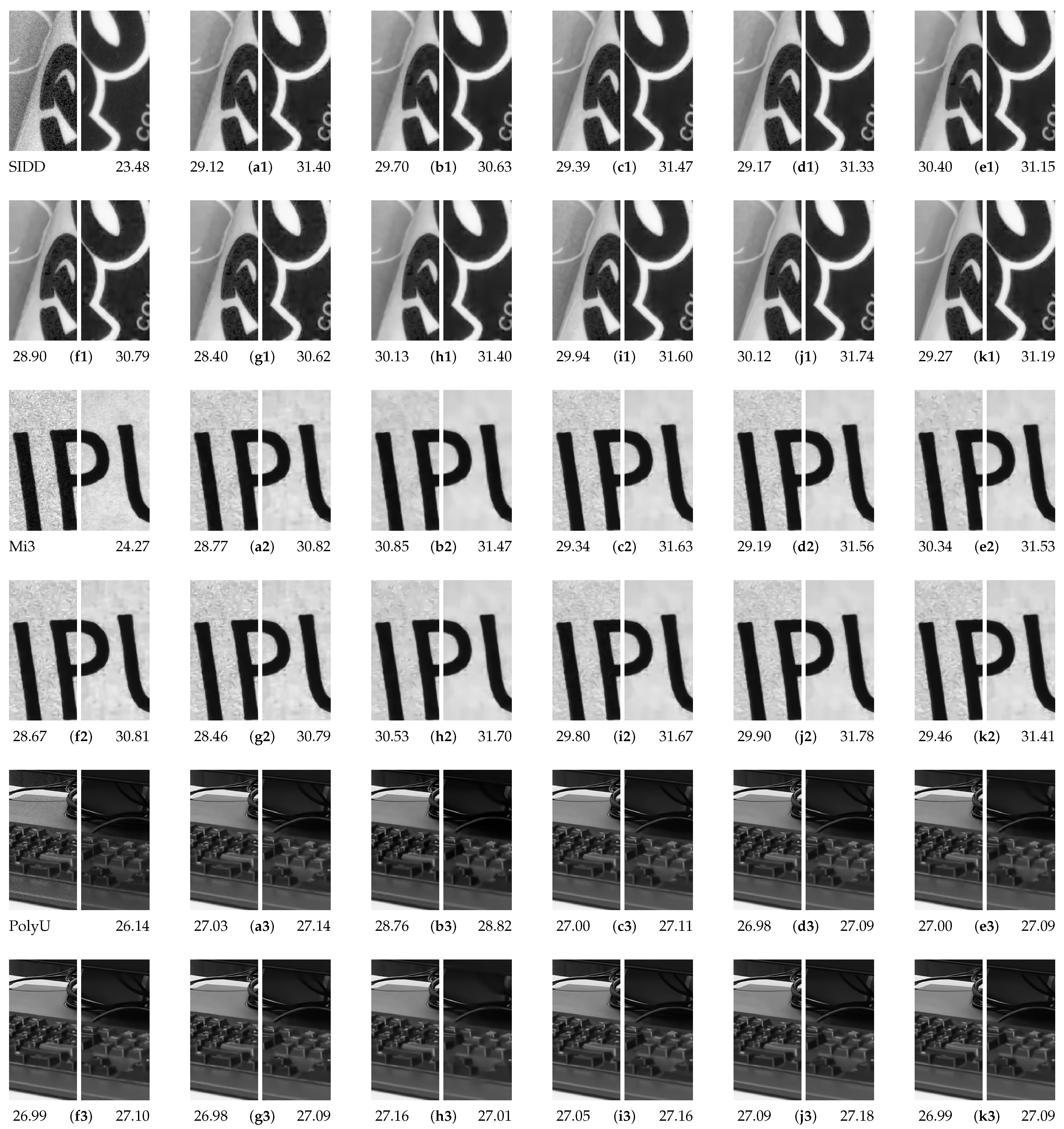
Figure 4 illustrates the results in Table 2. We can observe that the original denoising image $f_{\mathrm{de}}$ has heavy artifacts, although the pattern of $f_{\mathrm{de}}$ in different denoising methods are diverse, and there are strong correlations in noise between the pattern of $f_{\mathrm{noise}}$ and the corresponding $f_{\mathrm{de}}$, which proves that the Gaussian noise-based methods can not remove realistic noise well and those patterns mainly come from the low-frequency part of realistic noise, as analysed in Section 4. After the proposed extending method, the artifacts are well removed, $f_{\mathrm{out}}$ is much clearer in flat area, and the texture is not blurred compared with $f_{\mathrm{de}}$. The edge in $f_{\mathrm{out}}$ still remains sharp and does not have additional artifacts.

Through Table 2, we can see that some outdated denoising methods, such as NCSR [49], perform better after applying the proposed method rather than newly proposed methods like corr-BM3D [42], as even its original denoising results have lower PSNR. Table 3 presents the comparison between the denoising results of the Renoir dataset in Table 2 and the recently proposed realistic noise denoising methods which also include the deep learning-based methods.

NAFNet [51] and DRANet [52] are trained on the SIDD dataset, and SCUNet [53] is trained on multiple datasets with noise augmentation schemes. Because deep learning-based methods require training on denoising datasets while traditional methods do not, employing those methods to untrained scenarios can better demonstrate the generalization ability. We only compare the results of the deep learning-based methods which are not trained on Renoir dataset. We can see that the proposed extending method can make the Gaussian noise-based dneoising methods compatible with realistic noise removal methods. With the proposed extending method, NCSR [49] surpass NLH [54] and deep learning-based methods in the Mi3 category of the Renoir dataset, and ACPT [44] outperforms the other methods in SSIM in T3i.

Table 3. Comparison of the PSNR and SSIM of denoising results between the extending results and the realistic noise removal methods on the green channel of Renoir [23] datasets. The highest PSNR and SSIM are marked in red and the second highest are marked in blue.

	Mi3		T3i		S90
Methods	PSNR	SSIM	PSNR	SSIM	PSNR	SSIM
NLH [54]	35.23	0.2939	40.95	0.2539	34.92	0.3029
Bitonic Filter [55]	30.31	0.2304	33.50	0.1437	31.26	0.3288
DRANet-32 [52]	33.22	0.2708	38.01	0.2251	33.72	0.3574
NAFNet [51]	32.43	0.2526	35.99	0.2057	33.26	0.3474
SCUNet [53]	34.73	0.2849	39.53	0.2490	34.10	0.2968
ACPT [44] + Proposed	35.82	0.2264	39.65	0.2580	34.53	0.2710
NCSR [49] + Proposed	36.10	0.2174	39.80	0.2483	33.45	0.2596
TWSC [7] + Proposed	35.82	0.2192	39.70	0.2540	34.46	0.2688

Table 3. Comparison of the PSNR and SSIM of denoising results between the extending results and the realistic noise removal methods on the green channel of Renoir [23] datasets. The highest PSNR and SSIM are marked in red and the second highest are marked in blue.

	Mi3		T3i		S90
Methods	PSNR	SSIM	PSNR	SSIM	PSNR	SSIM
NLH [54]	35.23	0.2939	40.95	0.2539	34.92	0.3029
Bitonic Filter [55]	30.31	0.2304	33.50	0.1437	31.26	0.3288
DRANet-32 [52]	33.22	0.2708	38.01	0.2251	33.72	0.3574
NAFNet [51]	32.43	0.2526	35.99	0.2057	33.26	0.3474
SCUNet [53]	34.73	0.2849	39.53	0.2490	34.10	0.2968
ACPT [44] + Proposed	35.82	0.2264	39.65	0.2580	34.53	0.2710
NCSR [49] + Proposed	36.10	0.2174	39.80	0.2483	33.45	0.2596
TWSC [7] + Proposed	35.82	0.2192	39.70	0.2540	34.46	0.2688

6.3. Selection of Hyper-Parameters

The proposed method is calculated based on local image patches. The size and stride of patches and the converging threshold are selected manually. A large image patch requires more computational resources and contains too much information, which makes the amplification factor in the local patch variate excessively and can not be roughly considered as constant in local area as the assumption, while a small patch size does not reflect the amplification in noise perfectly due to the spatial correlation feature. However, as the datasets that are used for evaluation in this work are all of high resolutions, they require a very big patch size to make the assumption fail. Hence, in our experiments, a bigger patch size usually improves the PSNR of the results. What is more, a large stride can greatly reduce the computational cost while the small stride size has better denoising effects.

Table 4. PSNR of the results under patch sizes 4, 8, and 16, and strides 1, 2, and 4 on the green channel of the SIDD dataset and the corresponding processing time.

Methods	Stride	1			2			4
	Patch Size	4	8	16	4	8	16	4	8	16
Processing Time (s)		0.157	0.648	2.443	0.044	0.169	0.641	0.012	0.046	0.166
BM3D [2]		37.91	38.45	38.69	37.84	38.43	38.68	37.45	38.34	38.65
corr-BM3D [42]		38.19	38.27	38.48	38.13	38.25	38.45	37.81	38.16	38.43
ACPT [44]		38.11	38.67	38.86	38.02	38.65	38.86	37.46	38.54	38.84
ACVA [45]		37.92	38.58	38.83	37.83	38.56	38.82	37.28	38.45	38.75
gmm [46]		38.29	38.40	38.57	38.23	38.38	38.52	37.93	38.29	38.50
lmm [47]		37.76	38.28	38.45	37.68	38.26	38.45	37.29	38.17	38.40
ggmm [47]		37.72	38.26	38.43	37.65	38.24	38.42	37.22	38.14	38.36
KSVD [48]		38.34	38.39	38.43	38.27	38.37	38.41	37.87	38.26	38.38
PGPD [50]		38.08	38.69	38.90	37.99	38.67	38.90	37.44	38.56	38.82
NCSR [49]		38.57	38.98	39.15	38.48	38.96	39.12	37.99	38.86	39.10
TWSC [7]		38.28	38.66	38.80	38.21	38.65	38.79	37.84	38.56	38.75

shows the PSNR of $f_{\mathrm{out}}$ under patch size 4, 8, 12, and 16, and stride 1, 2, and 4, as well as the corresponding computation time. The patch size bigger than 16 requires a larger stride to make the overall processing time practical; hence, the biggest patch size we test is 16. There is a improvement in the denoising effect of almost all methods when the patch size increases each time, and the processing time is proportional to the size of the patch. In most methods, although under patch size 4 the PSNR drops rapidly as the stride increases, under patch size 16 the PSNR of stride 4 is only slightly lower than that of stride 1, while the processing speed is 15 times faster. Hence, the default patch and stride size of the proposed method are 16 and 4. From the processing time in Table 4, we can see that it takes about 14 s for an image with ten million pixels, and if we set the patch size to 8 with stride 4, the processing time will further reduce to less than 4 s.

Table 5. PSNR of the results of NCSR [49] in SIDD dataset under different hyper-parameter settings.

Parameter		p
		0	0.001	0.002	0.005	0.01
$\mathit{q}$	1	38.50	39.09	39.09	39.08	39.08
	0.99	38.48	39.09	39.09	39.08	39.08
	0.96	38.45	39.09	39.10	39.09	39.07
	0.9	38.40	39.08	39.08	39.07	39.06

shows the PSNR of $f_{\mathrm{out}}$ optimized from the results of NCSR [49] in SIDD dataset. The PSNR of results do not change rapidly with p and q, and the optimal result is obtained under default settings, which means the proposed method is not sensitive to parameter selection. However, the optimal parameter settings for different denoising methods and datasets are not invariant. The selection of the default setting is based on the overall performance of the presented methods in Table 2.

6.4. Comparison on Initial Value

As analysed in Section 5, we propose an initial value selection scheme to obtain a value closer to the minimum point than one to reduce the computational cost.

Table 6. Processing time with and without the proposed initial value selection scheme.

Initial Value for ${\mathit{a}}_{\mathit{ij}}$	Optimization Time	Processing Time (s)
proposed Equation (21)	0.115	0.166
$a_{ij}=1$	0.139	0.189

shows the processing time for the optimization with and without the selected initial value. We can see that the optimization time is reduced with the selected initial value. Note that the optimization time presented in Table 6 is not the same as in Table 4, because the overall processing time includes Guided Filtering, Fourier Transformation, optimization iteration and image patch aggregation, while the optimization process only contains the optimization iteration.

6.5. Characteristics of Image

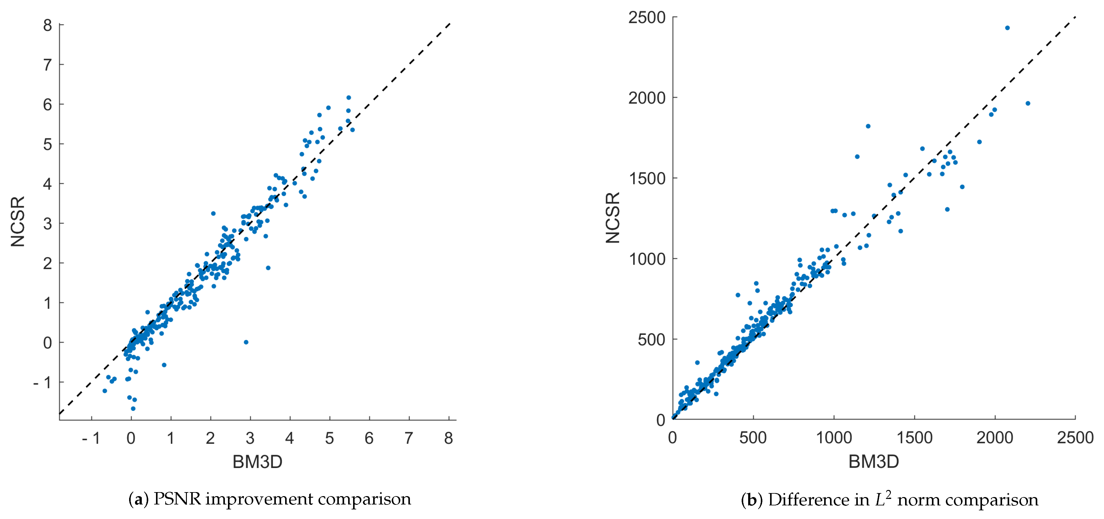
Figure 5 shows the comparisons between BM3D [2] and NCSR [49] on the PSNR improvement and ${\parallel f_{\mathrm{out}}-f_{\mathrm{de}}\parallel }_{L^2}$; each point denotes an image and almost all points are distributed around the straight line passing through the origin with slope one. The correlation coefficients between the PSNR improvement and the rest of the methods are also close to one, which means if one Gaussian noise-based denoising method can benefit much from the proposed method for some noisy image, other methods are also likely to benefit a lot for the same image.

This is because, as analysed in Section 3, the performance of Gaussian noise-based method on realistic noise is mainly impacted by the the spatial correlation of noise, which varies a lot in different images, as is presented in Figure 2. Hence, the noise left in the original denoising results that are obtained by different denoising methods exhibits certain similarities, since they can not handle spatially correlated noise, and the improvements brought by the extension are also similar due to the proposed method removing the correlated noise in the frequency domain.

6.6. Texture Preservation

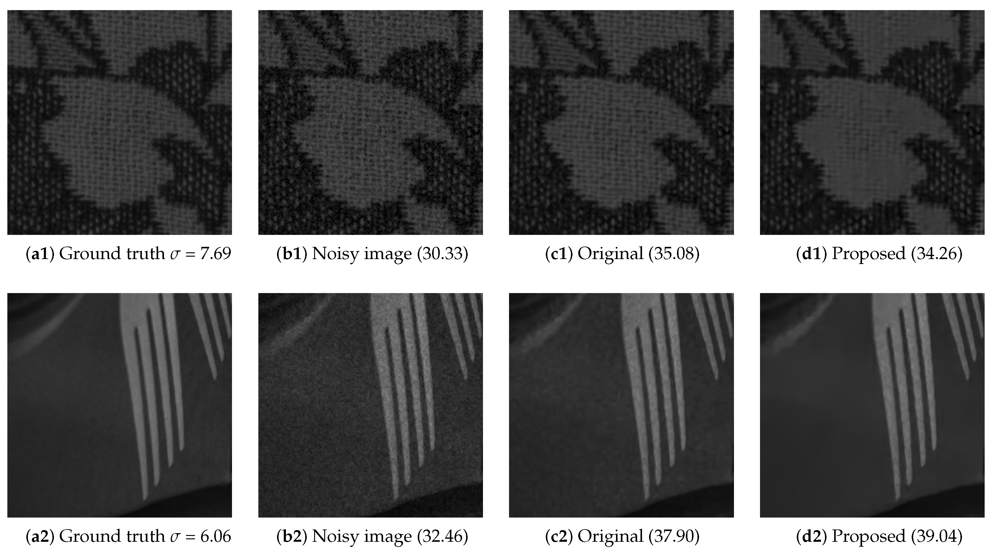
The proposed method removes the over-amplified noise in the frequency domain. However, apart from the spatial correlation within noise, the noise may also correlate to the noise-free image as well. In that case, the texture from the image may be falsely amplified due to the correlation of noise, and may cause the proposed method to over-smooth the image texture. Figure 6 shows the extending result from the NCSR method. We can observe that the proposed method can maintain the sharpness and continuity of long edges, but for the texture with very small scales, the proposed method cause blurriness in the texture aspect and result in a drop in PSNR.

6.7. Discussion

From the analysis in Section 4, we can see that despite the proposed method only adopting two different ${\mathsf{\ell }}_p$ norms, the optimization scheme can be directly generalized to a mix of three or more different concave norms. However, more complicated norms will increase the computation cost, though can not guarantee a better performance.

As presented in Table 2, the proposed method can facilitate different Gaussian noise-based denoising methods in realistic noise removal, which proves that there are great differences between Gaussian noise and realistic noise as well as the efficiency of the proposed method. We do not compare the denoising result of the SIDD [41] dataset in Table 3 because the deep learning-based methods we compared are trained on the SIDD dataset, which make them perform much better than in other datasets. Additionally, the proposed method does not perform well on the image with lower noise intensity; as presented in Table 2, there are almost no improvements in PolyU dataset. Hence, we can adopt an estimation scheme regarding the intensity of noise and the flatness of the original image to make the hyper-parameters adaptive to local patches in future works.

7. Conclusions

In this paper, we analysed the difference between Gaussian noise and realistic noise, and proposed a novel weighted, mixed ${\mathsf{\ell }}_p$ norm-based regularizer with its optimization scheme to extend the Gaussian noise-based denoising method to realistic denoising cases. Numerical experiments show that our method can extend Gaussian noise-based methods to mainstream realistic denoising datasets effectively, and even outdated denoising method may outperform recently proposed realist denoising methods with our proposed extending method.

However, because the proposed method focuses on removing spatially correlated noise, images with low noise intensity cannot benefit much from the proposed method. And, when the noise intensity is too strong and so heavily correlated that the noise in the original denoised image is barely removed, the proposed method would also not able to handle it well. In our future research, we will focus on the dealing with such situations and further generalize our work to RGB image denoising.

References

1. Panagiotou, S.; Bosman, A.S. Denoising diffusion post-processing for low-light image enhancement. Pattern Recognit. 2024, 156, 110799. [Google Scholar] [CrossRef] [Scilit]
2. Dabov, K.; Foi, A.; Katkovnik, V.; Egiazarian, K. Image Denoising by Sparse 3-D Transform-Domain Collaborative Filtering. IEEE Trans. Image Process. 2007, 16, 2080–2095. [Google Scholar] [CrossRef] [Scilit]
3. Basak, S.; Mukherjee, P.S. An efficient image denoising method integrating multi-resolution local clustering and adaptive smoothing: S. Basak, PS Mukherjee. In Statistical Methods & Applications; Springer: Berlin/Heidelberg, Germany, 2025; pp. 1–19. [Google Scholar]
4. Park, S.H.; Kim, H.S.; Lansel, S.; Parmar, M.; Wandell, B.A. A case for denoising before demosaicking color filter array data. In Proceedings of the Conference Record of the Forty-Third Asilomar Conference on Signals, Systems and Computers, Pacific Grove, CA, USA, 1–4 November 2009; pp. 860–864. [Google Scholar] [CrossRef] [Scilit]
5. Guo, S.; Yan, Z.; Zhang, K.; Zuo, W.; Zhang, L. Toward Convolutional Blind Denoising of Real Photographs. In Proceedings of the IEEE/CVF Conference on Computer Vision and Pattern Recognition, Long Beach, CA, USA, 15–20 June 2019; pp. 1712–1722. [Google Scholar] [CrossRef] [Scilit]
6. Lebrun, M.; Colom, M.; Morel, J.M. Multiscale Image Blind Denoising. IEEE Trans. Image Process. 2015, 24, 3149–3161. [Google Scholar] [CrossRef] [Scilit] [PubMed]
7. Xu, J.; Zhang, L.; Zhang, D. A Trilateral Weighted Sparse Coding Scheme for Real-World Image Denoising. In Proceedings of the European Conference on Computer Vision, Munich, Germany, 8–14 September 2018; pp. 21–38. [Google Scholar] [CrossRef] [Scilit]
8. Xu, J.; Huang, Y.; Cheng, M.M.; Liu, L.; Zhu, F.; Xu, Z.; Shao, L. Noisy-as-Clean: Learning Self-Supervised Denoising From Corrupted Image. IEEE Trans. Image Process. 2020, 29, 9316–9329. [Google Scholar] [CrossRef] [Scilit]
9. Luo, Y.; Zhao, X.; Meng, D. Revisiting Nonlocal Self-Similarity from Continuous Representation. IEEE Trans. Pattern Anal. Mach. Intell. 2025, 47, 450–468. [Google Scholar] [CrossRef] [Scilit]
10. Starck, J.L.; Candes, E.; Donoho, D. The curvelet transform for image denoising. IEEE Trans. Image Process. 2002, 11, 670–684. [Google Scholar] [CrossRef] [Scilit]
11. Liu, C.; Szeliski, R.; Bing Kang, S.; Zitnick, C.L.; Freeman, W.T. Automatic Estimation and Removal of Noise from a Single Image. IEEE Trans. Pattern Anal. Mach. Intell. 2008, 30, 299–314. [Google Scholar] [CrossRef] [Scilit]
12. Chi, Y.; Chan, S.H. Fast And Robust Recursive Filter for Image Denoising. In Proceedings of the IEEE Internatinal Conference on Acoustics, Speech and Signal Processing, Calgary, AB, Canada, 15–20 April 2018; pp. 1708–1712. [Google Scholar] [CrossRef] [Scilit]
13. Chen, S.; Liu, M.; Zhang, W.; Liu, J. Edge preserving image denoising with a closed form solution. Pattern Recognit. 2013, 46, 976–988. [Google Scholar] [CrossRef] [Scilit]
14. Berman, D.; Treibitz, T.; Avidan, S. Non-local Image Dehazing. In Proceedings of the IEEE/CVF Conference on Computer Vision and Pattern Recognition, Las Vegas, NV, USA, 27–30 June 2016; pp. 1674–1682. [Google Scholar] [CrossRef] [Scilit]
15. Yan, Z.; Guo, S.; Xiao, G.; Zhang, H. On Combining CNN With Non-Local Self-Similarity Based Image Denoising Methods. IEEE Access 2020, 8, 14789–14797. [Google Scholar] [CrossRef] [Scilit]
16. Beck, A.; Teboulle, M. Fast Gradient-Based Algorithms for Constrained Total Variation Image Denoising and Deblurring Problems. IEEE Trans. Image Process. 2009, 18, 2419–2434. [Google Scholar] [CrossRef] [Scilit] [PubMed]
17. Li, T.; Li, F.; Qi, H. A Weibull gradient prior for image restoration. J. Comput. Appl. Math. 2024, 439, 115594. [Google Scholar] [CrossRef] [Scilit]
18. Candès, E.J.; Wakin, M.B.; Boyd, S.P.; Boyd, S.P. Enhancing Sparsity by Reweighted 1 Minimization. J. Fourier Anal. Appl. 2008, 14, 877–905. [Google Scholar] [CrossRef] [Scilit]
19. Xiao, P.; Liao, B. Robust one-bit compressive sensing with weighted 1-norm minimization. Signal Process. 2019, 164, 380–385. [Google Scholar] [CrossRef] [Scilit]
20. Meng, J.; Zhang, H.; Yan, Z.; Liu, T.; Ma, X.; Wei, Z.; Yang, H. A reweighted 0-norm-constraint LMS algorithm for sparse system identification. Digit. Signal Process. 2022, 123, 103456. [Google Scholar] [CrossRef] [Scilit]
21. Berkessa, Z.A.; Waldmann, P. Weighted L1 and L0 Regularization Using Proximal Operator Splitting Methods. Trans. Mach. Learn. Res. 2024, 2024, 3029. [Google Scholar]
22. Bu, Y.; Zhao, Y.; Chan, J.C.W. Mixed norm regularized models for low-rank tensor completion. Inf. Sci. 2024, 670, 120630. [Google Scholar] [CrossRef] [Scilit]
23. Anaya, J.; Barbu, A. RENOIR – A dataset for real low-light image noise reduction [dataset]. J. Vis. Commun. Image Represent. 2018, 51, 144–154. [Google Scholar] [CrossRef] [Scilit]
24. Yin, K.; Zhao, H.; Lu, L. Functional link artificial neural network filter based on the q-gradient for nonlinear active noise control. J. Sound Vib. 2018, 435, 205–217. [Google Scholar] [CrossRef] [Scilit]
25. Korki, M.; Zayyani, H. Weighted diffusion continuous mixed p-norm algorithm for distributed estimation in non-uniform noise environment. Signal Process. 2019, 164, 225–233. [Google Scholar] [CrossRef] [Scilit]
26. Ma, W.; Duan, J.; Gui, G.; Chen, B. Robust diffusion recursive adaptive filtering algorithm based on lp-norm. In Proceedings of the 2016 35th Chinese Control Conference (CCC), Chengdu, China, 27–29 July 2016; pp. 1404–1408. [Google Scholar] [CrossRef] [Scilit]
27. Su, Y.; Li, Z.; Yu, H.; Wang, Z. Multi-band weighted lp norm minimization for image denoising. Inf. Sci. 2020, 537, 162–183. [Google Scholar] [CrossRef] [Scilit]
28. Xu, J.; Wang, N.; Xu, Z.; Xu, K. Weighted lp Norm Sparse Error Constraint Based ADMM for Image Denoising. Math. Probl. Eng. 2019, 2019, 1262171. [Google Scholar] [CrossRef] [Scilit]
29. Tan, Z.; Yang, H. Total variation regularized multi-matrices weighted Schatten p-norm minimization for image denoising. Appl. Math. Model. 2023, 124, 518–531. [Google Scholar] [CrossRef] [Scilit]
30. Sadraeifar, B.; Abedi, M. 3D inversion of gravity data using mixed Lp–Lq norm regularization, a case study for potash targeting at the Ghare-Aghaj deposit in Iran. Carbonates Evaporites 2024, 39, 66. [Google Scholar] [CrossRef] [Scilit]
31. Vatankhah, S.; Huang, X.; Renaut, R.A.; Mickus, K.; Kabirzadeh, H.; Lin, J. Efficiently Implementing and Balancing the Mixed Lp-Norm Joint Inversion of Gravity and Magnetic Data. IEEE Trans. Geosci. Remote Sens. 2023, 61, 1–17. [Google Scholar] [CrossRef] [Scilit]
32. Song, P.; Zhao, H. Filtered-x generalized mixed norm (FXGMN) algorithm for active noise control. Mech. Syst. Signal Process. 2018, 107, 93–104. [Google Scholar] [CrossRef] [Scilit]
33. Dong, W.; Shi, G.; Li, X. Nonlocal Image Restoration with Bilateral Variance Estimation: A Low-Rank Approach. IEEE Trans. Image Process. 2013, 22, 700–711. [Google Scholar] [CrossRef] [Scilit] [PubMed]
34. Liu, J.; Ni, A.; Ni, G. A nonconvex 1(1-2) model for image restoration with impulse noise. J. Comput. Appl. Math. 2020, 378, 112934. [Google Scholar] [CrossRef] [Scilit]
35. Gu, S.; Zhang, L.; Zuo, W.; Feng, X. Weighted Nuclear Norm Minimization with Application to Image Denoising. In Proceedings of the IEEE/CVF Conference on Computer Vision and Pattern Recognition, Columbus, OH, USA, 23–28 June 2014; pp. 2862–2869. [Google Scholar] [CrossRef] [Scilit]
36. Goossens, B.; Pizurica, A.; Philips, W. Removal of Correlated Noise by Modeling the Signal of Interest in the Wavelet Domain. IEEE Trans. Image Process. 2009, 18, 1153–1165. [Google Scholar] [CrossRef] [Scilit]
37. Wei, K.; Fu, Y.; Zheng, Y.; Yang, J.d. Physics-Based Noise Modeling for Extreme Low-Light Photography. IEEE Trans. Pattern Anal. Mach. Intell. 2022, 44, 8520–8537. [Google Scholar] [CrossRef] [Scilit]
38. He, K.; Sun, J.; Tang, X. Guided Image Filtering. IEEE Trans. Pattern Anal. Mach. Intell. 2013, 35, 1397–1409. [Google Scholar] [CrossRef] [Scilit]
39. Boyd, S.; Xiao, L.; Mutapcic, A. Subgradient Methods; Lecture Notes of EE392o; Autumn Quarter 2003–2004; Stanford University: Stanford, CA, USA, 2003. [Google Scholar]
40. Lin, R.; Li, S.; Li, Z.; Liu, Y. Convergence analysis of iteratively reweighted 1 algorithms for computing the proximal operator of p-norm. Math. Methods Appl. Sci. 2025, 48, 386–396. [Google Scholar] [CrossRef] [Scilit]
41. Abdelhamed, A.; Lin, S.; Brown, M.S. A High-Quality Denoising Dataset for Smartphone Cameras [dataset]. In Proceedings of the IEEE/CVF Conference on Computer Vision and Pattern Recognition, Salt Lake City, UT, USA, 18–23 June 2018; pp. 1692–1700. [Google Scholar] [CrossRef] [Scilit]
42. Mäkinen, Y.; Azzari, L.; Foi, A. Collaborative Filtering of Correlated Noise: Exact Transform-Domain Variance for Improved Shrinkage and Patch Matching. IEEE Trans. Image Process. 2020, 29, 8339–8354. [Google Scholar] [CrossRef] [Scilit]
43. Benesty, J.; Chen, J.; Huang, Y. Study of the widely linear Wiener filter for noise reduction. In Proceedings of the IEEE International Conference on Acoustics, Speech and Signal Processing, Dallas, TX, USA, 14–19 March 2010; pp. 205–208. [Google Scholar] [CrossRef] [Scilit]
44. Zhao, W.; Lv, Y.; Liu, Q.; Qin, B. Detail-Preserving Image Denoising via Adaptive Clustering and Progressive PCA Thresholding. IEEE Access 2018, 6, 6303–6315. [Google Scholar] [CrossRef] [Scilit]
45. Zhao, W.; Liu, Q.; Lv, Y.; Qin, B. Texture Variation Adaptive Image Denoising With Nonlocal PCA. IEEE Trans. Image Process. 2019, 28, 5537–5551. [Google Scholar] [CrossRef]
46. Zoran, D.; Weiss, Y. From learning models of natural image patches to whole image restoration. In Proceedings of the International Conference on Computer Vision, Barcelona, Spain, 6–13 November 2011; pp. 479–486. [Google Scholar] [CrossRef] [Scilit]
47. Deledalle, C.A.; Parameswaran, S.; Nguyen, T.Q. Image Denoising with Generalized Gaussian Mixture Model Patch Priors. SIAM J. Imaging Sci. 2018, 11, 2568–2609. [Google Scholar] [CrossRef] [Scilit]
48. Elad, M.; Aharon, M. Image Denoising Via Sparse and Redundant Representations Over Learned Dictionaries. IEEE Trans. Image Process. 2006, 15, 3736–3745. [Google Scholar] [CrossRef] [Scilit]
49. Dong, W.; Zhang, L.; Shi, G.; Li, X. Nonlocally Centralized Sparse Representation for Image Restoration. IEEE Trans. Image Process. 2013, 22, 1620–1630. [Google Scholar] [CrossRef] [Scilit]
50. Xu, J.; Zhang, L.; Zuo, W.; Zhang, D.; Feng, X. Patch Group Based Nonlocal Self-Similarity Prior Learning for Image Denoising. In Proceedings of the IEEE/CVF International Conference on Computer Vision, Santiago, Chile, 7–13 December 2015; pp. 244–252. [Google Scholar] [CrossRef] [Scilit]
51. Chen, L.; Chu, X.; Zhang, X.; Sun, J. Simple baselines for image restoration. In Proceedings of the European Conference on Computer Vision, Tel Aviv, Israel, 23–27 October 2022; Springer: Berlin/Heidelberg, Germany, 2022; pp. 17–33. [Google Scholar] [CrossRef] [Scilit]
52. Wu, W.; Liu, S.; Xia, Y.; Zhang, Y. Dual residual attention network for image denoising. Pattern Recognit. 2024, 149, 110291. [Google Scholar] [CrossRef] [Scilit]
53. Zhang, K.; Li, Y.; Liang, J.; Cao, J.; Zhang, Y.; Tang, H.; Fan, D.P.; Timofte, R.; Gool, L.V. Practical blind image denoising via Swin-Conv-UNet and data synthesis. Mach. Intell. Res. 2023, 20, 822–836. [Google Scholar] [CrossRef] [Scilit]
54. Hou, Y.; Xu, J.; Liu, M.; Liu, G.; Liu, L.; Zhu, F.; Shao, L. NLH: A Blind Pixel-Level Non-Local Method for Real-World Image Denoising. IEEE Trans. Image Process. 2020, 29, 5121–5135. [Google Scholar] [CrossRef] [Scilit]
55. Treece, G. Real Image Denoising With a Locally-Adaptive Bitonic Filter. IEEE Trans. Image Process. 2022, 31, 3151–3165. [Google Scholar] [CrossRef] [Scilit] [PubMed]
Figure 1. Overall structure of the proposed extending method. The frequency suppression scheme is presented in Algorithm 1.
Mathematics 14 00298 g001
Figure 2. From left to right are (a) ground truth f gt , (b) noisy image f noise , (c) original denoised image f de and (d) Guided filtering result f guid . The corresponding noise PSDs are presented in the up right corner.
Mathematics 14 00298 g002
Figure 3. Φ ( t ) and its derivative ϕ ( t ) in Equation (12) under different λ p and λ q where p = 0.1 and q = 0.95 . From (a) to (d), the sub-figures correspond to the situation of (a) ϕ ( t ^ ) < 0 , Φ ( t b ) < Φ ( 0 ) ; (b) ϕ ( t ^ ) < 0 , Φ ( t b ) > Φ ( 0 ) ; (c) ϕ ( t ^ ) = 0 ; and (d) ϕ ( t ^ ) > 0 . The minimum point of (a) is t b and zero in the rest of the sub-figures.
Mathematics 14 00298 g003
Figure 4. Denoising results of different methods on SIDD [41], Renoir [23] and PolyU datasets. In each sub-figure, on the left is the PSNR of original denoising result, and on the right is the PSNR of extended result. (a1a3) BM3D [2], (b1b3) corr-BM3D [42], (c1c3) ACPT [44], (d1d3) ACVA [45], (e1e3) gmm [46], (f1f3) lmm [47], (g1g3) ggmm [47], (h1h3) KSVD [48], (i1i3) PGPD [50], (j1j3) NCSR [49], and (k1k3) TWSC [7].
Mathematics 14 00298 g004
Figure 5. On the left (a) is the scatter diagram of PSNR improvement of each image in BM3D [2] and NCSR [49]. On the right (b) is the comparisons of f out f de L 2 . The dashed line pass through the origin with slope one is used for comparison.
Mathematics 14 00298 g005
Figure 6. Denoising results of the proposed method under different image textures. The number in the bracket denotes its PSNR and the number under ground truth image denotes the standard deviation of noise.
Mathematics 14 00298 g006