Constructing Two Edge-Disjoint Hamiltonian Cycles in BCube Data Center Networks for All-to-All Broadcasting

Abstract

The rapid growth in demand for diverse network application services has driven the continuous development and expansion of data centers. BCubes was proposed by Microsoft Research Asia for designing modular data centers, and it is a multi-layer recursively constructed network with many advantages. This article shows that BCube is the existence of two edge-disjoint Hamiltonian cycles, abbreviated as two EDHCs, which provide two significant benefits in data center operations: (1) parallel data broadcast and (2) edge fault-tolerance in network communications. We present the following results in this paper: (1) By utilizing the network topology characteristics, we first provide construction algorithms for two EDHCs on low-dimensional BCubes. (2) Based on the algorithm and the recursive structure of BCubes, we prove that two EDHCs exist for all BCubes. (3) Considering all-to-all broadcasting using two EDHCs as transmission channels, we evaluate the performance of all-to-all broadcasting through simulations on low-dimensional BCubes.

1. Introduction

Today’s users rely on a wide variety of network services every day. Consequently, data centers have emerged, consisting of numerous servers, storage devices, and network equipment within computer rooms. Due to the increasing popularity of cloud computing and the explosive growth of data, the scale of data center networks continues to grow, and this trend is becoming increasingly significant [1,2,3]. Data center networks play a crucial role in cloud computing and big data processing, and the design of the data center network connecting these devices is a crucial issue.

Due to the different transmission mechanisms of data center networks, they can be divided into switch-centric and server-centric. In a switch-centric data center network, the switch is mainly responsible for the routing to transmit packets between servers, while the server is only responsible for sending and receiving data packets. For example, Fat-Tree [4] is a typical example of this type. It uses a tree-like hierarchical structure of switches (including core switches, aggregation switches, and top-of-rack switches) to connect servers. Currently, the Fat-Tree topology has been widely adopted by many large companies such as Google [5] and Facebook [6]. In a server-centric data center network, the server is responsible for integrating all functions of the network. They are not only the source and destination of data transmission, but also act as path relay nodes, while all switches only act as transmission switches for forwarding packets. For example, BCube [7], DCell [8], FiConn [2], and HSDC [3] are the most typical architectures of this type.

An important issue in data center networks is to provide efficient routing for data transmission. Therefore, many problems in graph theory are also brought to the discussion of data center networks. In 2015, Wang et al. proved that a k-layer DCell data center network consisting of network switches with n transmission ports is Hamiltonian connected [9], where k ≥ 0 and n ≥ 2. Subsequently, Qin and Hao continued to study the above results, considering more fault edges, and proved that there exists a Hamiltonian cycle with conditional edge fault tolerance except for certain conditions [10]. In 2018, He et al. described the Hamiltonian cycle and scalability of the BCCC data center network, and the important role of the Hamiltonian cycle and scalability in network traffic [11]. Wang et al. studied the Hamiltonian cycle and Hamiltonian connectivity of the BCube data center network and considered server, network switch and link failures [12].

Ring structures are crucial for high-performance computing architectures and are often used as the baseband for data transmission in internetworks and for control flow in parallel and distributed environments. Many efficient algorithms based on ring structures with low communication costs have been developed [13,14]. A Hamiltonian cycle in a graph is a cycle (or ring) that visits each vertex exactly once. K (≥2) Hamiltonian cycles in a graph are said to be edge-disjoint if they have no common edges. The existence of edge-disjoint Hamiltonian cycles, abbreviated EDHCs, provides an advantage for implementing algorithms that require a ring structure, as it allows message traffic to be evenly distributed across the network. Furthermore, EDHCs also provide the edge-fault-tolerant hamiltonicity of an interconnection network.

Several studies have investigated the construction of EDHCs in various network topologies. Rowley and Bose [15] showed that slightly modified degree-2r de Bruijn networks can be decomposed into r Hamiltonian cycles when r is a power of a prime. Barth and Raspaud [16] demonstrated that butterfly graphs contain two EDHCs using a recursive construction method. In mesh and hypercube networks, Lee and Shin [13] leveraged EDHCs to achieve reliable all-to-all broadcasting. Bae and Bose [17] presented constructions of EDHCs in k-ary n-cube and hypercubes using Lee distance Gray codes. Petrovic and Thomassen [18] characterized the number of EDHCs in hypertournaments.

Other works focused on hypercube variants and related networks. Hung et al. constructed multiple EDHCs in locally twisted cubes [19], twisted cubes [20], augmented cubes [21], transposition networks, and general hypercube-like networks [22]. Wang et al. [23] proved that the n-dimensional parity cube (n ≥ 4) contains two EDHCs. Hussain et al. [24] showed how to generate three EDHCs in Eisenstein-Jacobi networks, while Albader and Bose [25] demonstrated the existence of two EDHCs in Gaussian networks. Furthermore, Pai et al. presented constructions of three EDHCs in locally twisted cubes [26], crossed cubes [27], folded locally twisted cubes [28], and folded crossed cubes [28].

Overall, these studies illustrate that EDHCs can be constructed in a wide variety of interconnection networks, but the number of EDHCs, construction methods, and underlying topological requirements differ across network families. However, since the Hamiltonian cycle problem is well known to be NP-complete for general graphs, such constructions typically rely on carefully exploiting the structural properties of specific network topologies. In this context, the present study focuses on BCube networks, providing explicit constructions of two EDHCs for all dimensions and arbitrary n. This contributes to both theoretical understanding and practical applicability in data center network designs.

The rest of the paper is organized as follows: Section 2 introduces the structures of BCube and its logic graph—generalized hypercube—and provides some notations. In Section 3, we show how to embed two EDHCs in Bcubes and present the construction algorithm and its proof. The two EDHCs have the advantage of allowing message traffic to be evenly distributed across the network. Some broadcasting simulations and the performance evaluation in low-dimensional BCubes are presented in Section 4. Finally, Section 5 presents the concluding remarks of this paper.

2. Preliminaries

The topology of a data center network can be modeled using a graph, where vertices represent servers and various devices, and edges represent network links. Let G = (V(G), E(G)) be a finite, simple, undirected graph, where V(G) is the vertex set of graph G, and E(G) is the edge set of graph G. The neighborhood of a vertex v in a graph G, denoted by N(v), is the set of vertices adjacent to v in G. A path P_m of length m in G, denoted by v₁–v₂–v₃–…–v_m−1–v_m, is a sequence (v₁, v₂, v₃, …, v_m−1, v_m) of vertices such that (v_i, v_i+1) ∈ E(G) for 1 ≤ i ≤ m − 1. A cycle C_m of length m in G, denoted by v₁–v₂–v₃–…–v_m−1–v_m–v₁, is a sequence (v₁, v₂, v₃, …, v_m−1, v_m, v₁) of vertices such that (v_m, v₁) ∈ E(G) and (v_i, v_i+1) ∈ E(G) for 1 ≤ i ≤ m − 1. To avoid ambiguity in the pseudocode and proofs, the operators used in this paper are summarized in

Table 1. List of operators used in the pseudocode and proofs.

Operator	Name	Definition	Example
⊕	Concatenation operator	Concatenates two symbols or labels to form a single label	3 ⊕ 5 = 35
+	Arithmetic addition	General numerical addition	1 + 7 = 8
mod	Modulo operator	Computes the remainder after integer division.	8 mod 5 = 3

. In particular, the operator ⊕ denotes label concatenation and should not be confused with arithmetic addition, whereas + and mod represent general numerical addition and modulo operations, respectively. These definitions are consistently applied throughout the construction and analysis of the proposed algorithms. For simplicity, the terms network and graph, node and vertex, as well as link and edge are used interchangeably in this paper.

In 2009, BCube was proposed by Microsoft Research Asia for designing modular data centers, and its prototype has been implemented on a testbed [7]. BCube is a multi-layer recursively constructed network with advantages such as low diameter, large bidirectional bandwidth, abundant parallel paths, and high aggregate data throughput. Since BCube can use a large number of general-purpose commercial servers and low-end switches with multiple network interfaces, it is a very advantageous choice in data center networks due to its low construction cost.

The BCube [7], denoted as BCube(n, k), can be described by two parameters n and k. First, BCube(n, 0) is the basic building block, where n represents an n-port switch and the number of connected servers. Then the parameter k is the number of levels, that is, the number of times the application network is recursively constructed. That is, BCube(n, k) is composed of n BCube(n, k − 1) and an additional n^k switches. There are n^k+1 k + 1-port servers and (k + 1)n^k n-port switches in one BCube(n, k). All switches are divided into k + 1 levels, and each level in BCube(n, k) has n^k switches. According to its design principle, each k + 1-port server must connect to switches at each level through one of its ports. In BCube(n, k), let a_ka_k−1…a₁a₀ be the addresses of servers, and ls_k−1…s₁s₀ be the addresses of switches at layer l, when a_i, s_i ∈ [0, n − 1] and l ∈ [0, k]. For the connection rules between switches and servers in BCube(n, k), please refer to Definition 1 below. 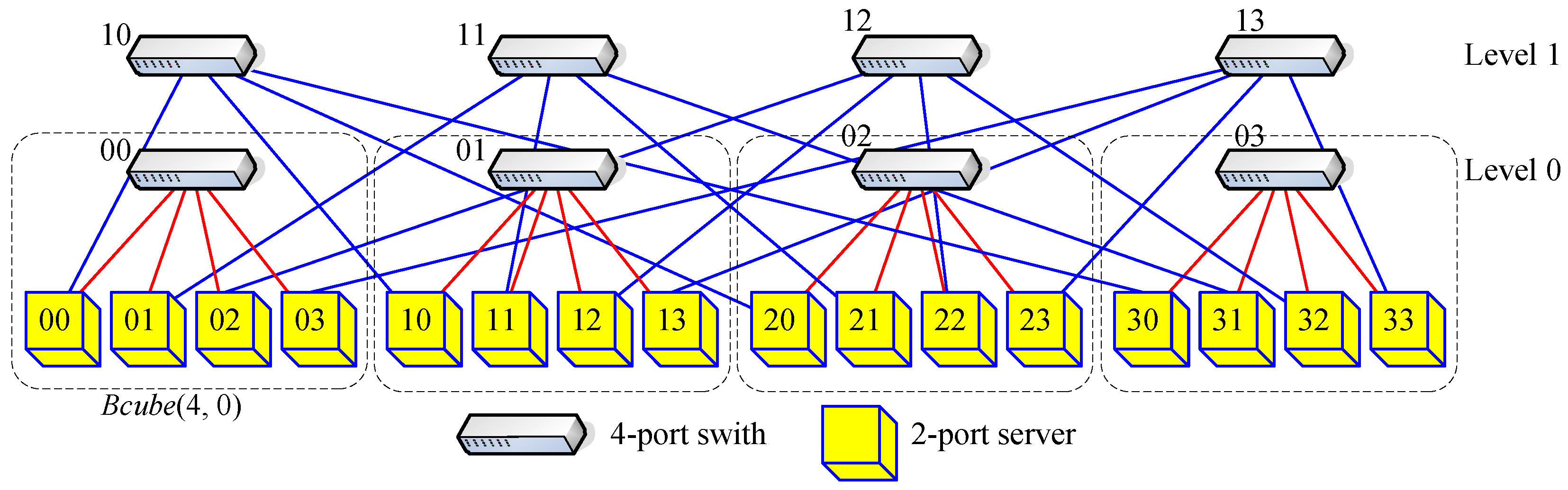Figure 1 is an example of BCube(4, 1).

Definition 1

([7]). BCube(n, k) is a recursively defined structure.

(1)

k = 0, BCube(n, 0) is simply n servers connecting to an n-port switch.

(2)

k ≥ 0, BCube(n, k) is constructed from n BCube(n, k − 1) and n^k n-port switches. The i-th port of level-l switch ls_k−1…s₁s₀ connects to l-th port of server a_ka_k−1…a₁a₀ where a_k = i, a_j = s_j for all j ∈ [0, k − 1] and l ∈ [0, k].

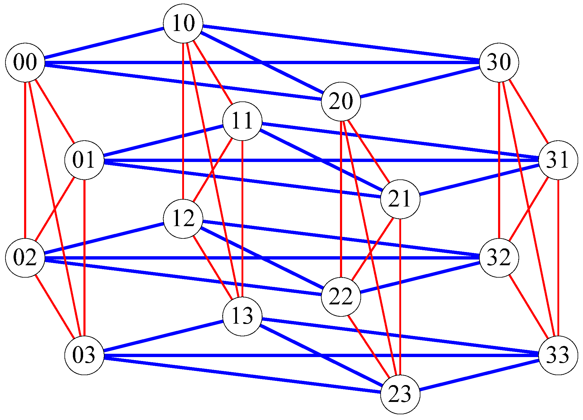
In particular, the logic graph of BCube(n, k) is actually a generalized hypercube GH(m_k, m_k−1, …, m₁, m₀) with all m_i = n and i ∈ [0, k]. The definition of the generalized hypercube [29] can be described as follows. For example, Figure 2 presents the logic graph GH(4, 4) of BCube(4, 1).

Definition 2 ([29]).

A r-dimensional generalized hypercube, denoted by GH(m_r−1, m_r−2,…, m₀) (r ≥ 1, m_i ≥ 2), is defined as follows:

(1)

The vertex set V(GH(m_r−1, m_r−2,…, m₀)) is a collection of all the r-dimension strings u_r−1u_r−2 ··· u₁u₀, where u_i ∈ [0, m_i − 1] for all 0 ≤ i ≤ r − 1.

(2)

For two vertices u and v, (u, v) ∈ E(GH(m_r−1, m_r−2,…, m₀)) if and only if their strings differ at exactly one dimension position.

BCube networks possess several structural properties that make them distinct from other interconnection networks. Unlike standard hypercubes or mesh networks, BCube is recursively defined and consists of multiple levels of servers connected through switches, which results in nontrivial connectivity patterns. This recursive and hierarchical structure creates unique challenges for constructing EDHCs, particularly when the number of servers n at each level is odd. Specifically, connecting the Hamiltonian cycles across the multiple BCube(n, k − 1) components requires careful coordination to ensure that the cycles remain edge-disjoint, and special treatment is needed for the last few components to maintain the Hamiltonian property. These challenges do not arise in more regular topologies such as hypercubes, meshes, or butterfly networks, where the symmetry and uniformity simplify EDHC construction.

3. Two EDHCs in BCube(n, k)

In this section, we first solve EDHCs on BCube(n, 0). Since the logic graph GH(n) of BCube(n, 0) is a complete graph K_n with n vertices, it is well known that there are ⌊${\displaystyle \frac{n-1}{2}}$⌋ EDHCs on K_n. This leads to the following lemma:

Lemma 1.

There exist ⌊ ${\displaystyle \frac{n-1}{2}}$⌋ EDHCs on BCube(n, 0) while n ≥ 5.

For convenience, since the logic graph of BCube(n, k) is the generalized hypercube GH(m_k, m_k−1, …, m₁, m₀) with k ≥ 1, all m_i = n and 1 ≤ i ≤ k, Figure 3, Figure 4, Figure 5, Figure 6, Figure 7, Figure 8 and Figure 9 below will use GH(m_k, m_k−1, …, m₁, m₀) instead of BCube(n, k). Next, we begin solving two EDHCs on BCube(n, 1).

Lemma 2.

There exist two EDHCs on BCube(3, 1).

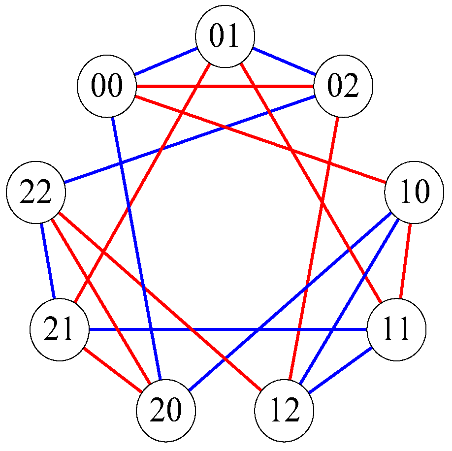
Proof of Lemma 2.

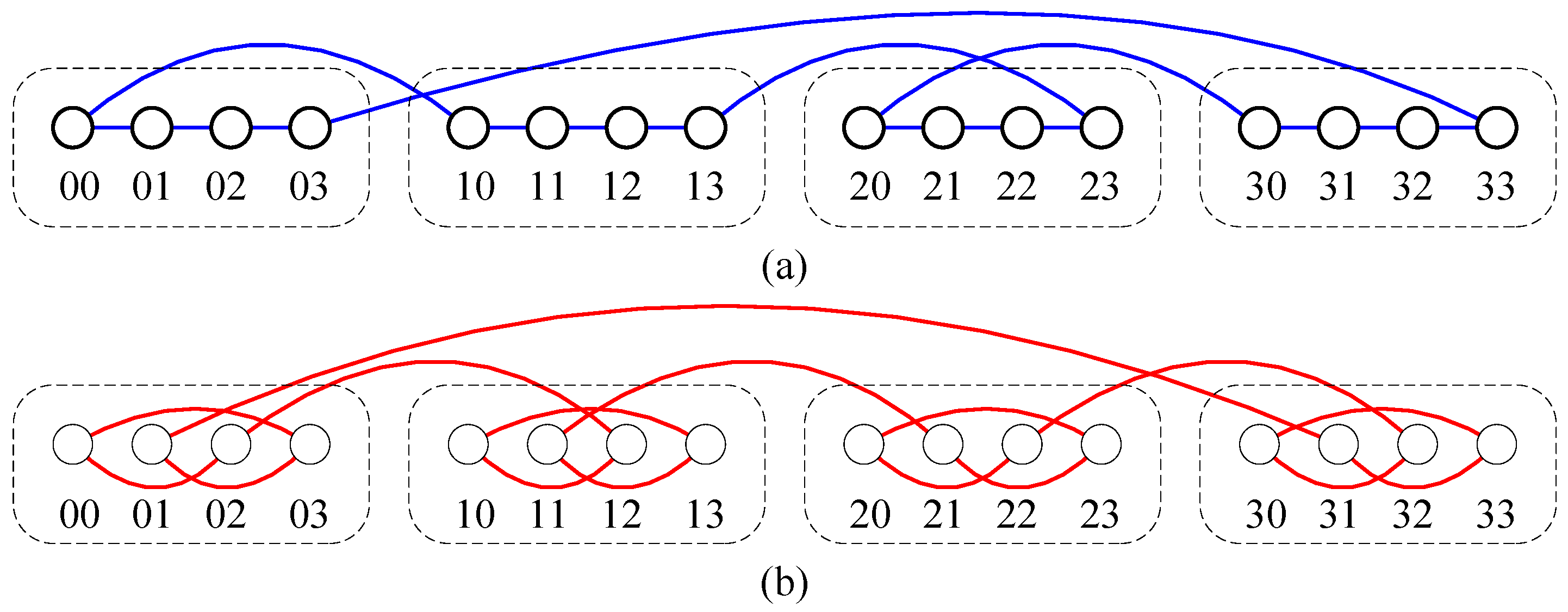
On the logic graph GH(3, 3) of BCube(3, 1), the two cycles 00-01-02-22-21-11-12-10-20-00 and 00-02-12-22-20-21-01-11-10-00 both pass through every vertex exactly once and share no common edges. These two cycles are depicted in Figure 3, which we can verify visually. Therefore, this lemma holds. □

Next, we solve two EDHCs on BCube(n, 1) when n ≥ 4. According to Definition 1, BCube(n, 1) is formed by adding new edges to n BCube(n, 0). Therefore, we first propose Lemma 3 to solve two edge-disjoint Hamiltonian paths on BCube(n, 0). Then, we concatenate all first (respectively, second) edge-disjoint Hamiltonian paths of n BCube(n, 0) to form the first (respectively, second) EDHC on BCube(n, 1).

Lemma 3.

There exist two edge-disjoint Hamiltonian paths on BCube(n, 0) for n ≥ 4.

Proof of Lemma 3.

According to Definition 2, the logic graph GH(n) of BCube(n, 0) is isomorphic to the complete graph K_n. The following proof is provided separately for whether n is odd or even.

Case 1: When n is even, the two paths 0-1-2-3-…-(n − 2)-(n − 1) and 1-3-5-…-(n − 3)-(n − 1)-0-2-4-…-(n − 4)-(n − 2) both pass through every vertex in the GH(n) once. For notational convenience, all vertex labels or arithmetic applied to GH(n) are taken modulo n. When 0 ≤ x ≤ n, the first path uses the edge (x, x + 1), and the second one uses the edge (x, x + 2) and the only edge (x, x + 1), which is (n − 1, 0). However, this edge is not used by the former, so these two paths are edge-disjoint Hamiltonian paths.

Case 2: When n is odd, the two paths 0-1-2-3-…-(n − 2)-(n − 1) and ⌊n/2 − 1⌋-⌊n/2 − 3⌋-⌊n/2 − 5⌋-…-⌊n/2 + 3⌋-⌊n/2 + 1⌋ both pass through every vertex in the GH(n) once. Furthermore, the former uses the edge (x, x + 1) and the latter uses the edge (x, x + 2), where 0 ≤ x ≤ n, so they do not share any common edges. □

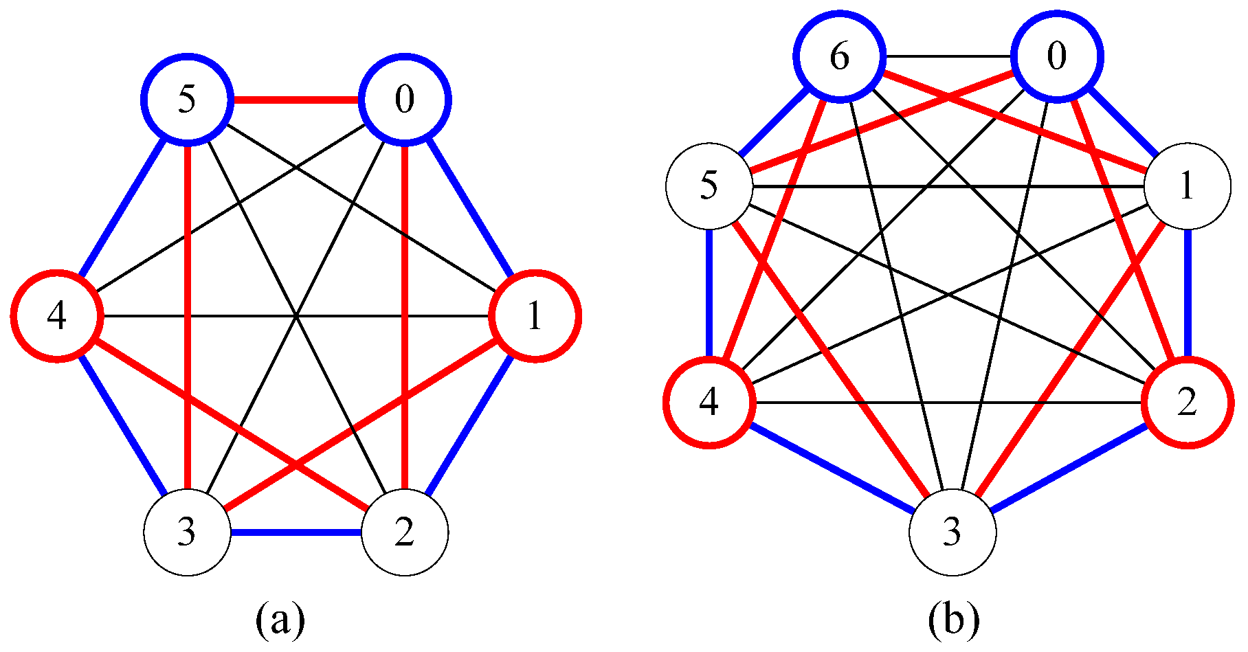
For example, Figure 4a shows two edge-disjoint Hamiltonian paths 0-1-2-3-4-5 and 1-3-5-0-2-4 on the logic graph GH(6) of BCube(6, 0), and Figure 4b shows two edge-disjoint Hamiltonian paths 0-1-2-3-4-5-6 and 2-0-5-3-1-6-4 on the logic graph GH(7) of BCube(7, 0).

Next, we will show how to construct two EDHCs on BCube(n, 1) while n ≥ 4. The parity of n affects the cycle construction method, so we first describe the construction algorithm for n being even, as follows (Algorithm 1):

Algorithm 1. 2EDHC_even(n)

Input: n Output: two edge-disjoint Hamiltonian cycles lists 1.     list1 = [ ]; list2 = [ ]; 2.     v ← [n − 1, n − 2, …, 2, 1, 0]; 3.     for g = 0 to n − 1 do 4.         for each x in v do 5.               append g ⊕ x to list1;    // ⊕ is a concatenated operator 6.         v ← reverse(v);                    // reverse list v 7.     v ← [1-3-5-…-(n − 3)-(n − 1)-0-2-4-…-(n − 4)-(n − 2)]; 8.     for g = 0 to n − 1 do 9.         for each x in v do 10.             append g ⊕ x to list2;    // ⊕ is a concatenated operator 11.       v ← reverse(v);                    // reverse list v 12. return list1, list2;

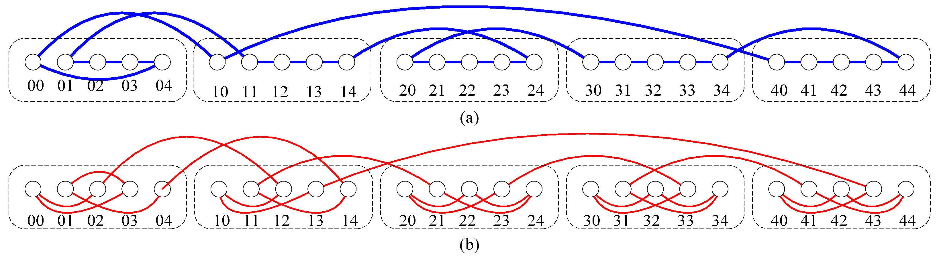
According to Definition 1, BCube(n, 1) consisted of n BCube(n, 0). In steps 2 and 7 of Algorithm 1, two edge-disjoint Hamiltonian paths are prepared on BCube(n, 0), as described in Lemma 3. Steps 3 to 6 and Steps 8 to 11, respectively, connect Hamiltonian paths of all n BCube(n, 0) into a Hamiltonian cycle on BCube(n, 1). For example, when n = 4, according to Algorithm 1, we can get 2 EDHCs 03-02-01-00-10-11-12-13-23-22-21-20-30-31-32-33-03 and 01-03-00-02-12-10-13-11-21-23-20-22-32-30-33-31-01 on BCube(4, 1), as shown in Figure 5.

Algorithm 1 consists of two main phases for constructing list1 and list2. In each phase, there is an outer loop iterating n times (Steps 3 and 8). Inside each outer loop, the algorithm traverses a list v of length n (Steps 4 and 9), and each iteration performs a constant-time append operation. The reverse(v) operation (Steps 6 and 11) also takes O(n) time and is executed n times. Therefore, the time complexity is O(n²). Both list1 and list2 store exactly n² vertex labels, corresponding to the vertices of BCube(n, 1). The auxiliary list v stores n elements. Hence, the space complexity is O(n²).

Next, we need to prove that the edges of the two Hamiltonian cycles constructed by the algorithm are edge-disjoint, so we propose the following lemma.

Lemma 4.

There exist two EDHCs on BCube(n, 1) for even n ≥ 4.

Proof of Lemma

4. According to Lemma 3, the two Hamiltonian paths in each BCube(n, 0) are edge-disjoint. Then, the endpoints of the first Hamiltonian path are 0 and (n − 1), and the endpoints of the second Hamiltonian path are 1 and (n − 2). Because of the different endpoints, the edges used by these two Hamiltonian cycles to connect n BCubes(n, 0) are also different. Therefore, according to Algorithm 1, two EDHCs can be obtained. □

Next, we give the construction algorithm when n is odd, as follows (Algorithm 2):

Algorithm 2. 2EDHC_odd(n)

Input: n Output: two edge-disjoint Hamiltonian cycles lists 1.       v ← [n − 1, n − 2, …, 2, 1, 0]; 2.       list1 = [0]; 3.       for x = n − 1 to 1 do            // visit all vertices in the first BCube(n, 0) 4.           append 0 ⊕ x to list1;    // ⊕ is a concatenated operator 5.       for x = 1 to n do        // visit all vertices except vertex 10 in the second BCube(n, 0) 6.           append 1 ⊕ x to list1;    // ⊕ is a concatenated operator 7.       for g = 2 to n − 1 do 8.           for each x in v do 9.                 append g ⊕ x to list1; 10.         v ← reverse(v);              // reverse list v 11.     append 10 to list1;            // visit vertex 10 12.     v ← [⌊n/2 − 1⌋, ⌊n/2 − 3⌋, ⌊n/2 − 5⌋, …, ⌊n/2 + 3⌋, ⌊n/2 + 1⌋]; 13.     cntr ← ⌊n/2⌋; list2 = [cntr]; // start from cntr 14.     for x = 1 to n − 1 do          // walk along (x, x − 2), visit all vertices in 1st BCube(n, 0) 15.         append 0 ⊕ (cntr − 2x) mod n to list2;    // mod is a modular operator 16.     for i = 1 to ⌊n/2⌋ do                      // visit ⌊n/2⌋ vertices in 2rd BCube(n, 0) 17.         x = (cntr + 2i) mod n 18.         append 1 ⊕ x to list2; 19.       for g = 2 to n − 1 do 20.           for each x in v do 21.                 append g ⊕ x to list2; 22.           v ← reverse(v); 23.     for i = ⌊n/2⌋ + 1 to n do      // visit remaining ⌊n/2⌋ + 1 vertices in 2rd BCube(n, 0) 24.         x = (cntr + 2i) mod n 25.         append 1 ⊕ x to list2; 26.     return list1, list2;

Steps 1 to 11 of this algorithm produce the first Hamiltonian cycle, and steps 12 to 25 generate the second one. To describe in more detail, steps 2 to 6 and 13 to 18 will visit all vertices in the first BCube(n, 0) and most of the vertices in the second BCube(n, 0). Then steps 7 to 10 and 19 to 22 continue to traverse all vertices in the remaining n BCube(n, 0). Finally, steps 11 and 23 to 25 continue to visit unvisited vertices in the second BCube(n, 0) and return to the starting vertex. Thus, two Hamiltonian cycles are obtained. For example, when n = 5, according to Algorithm 2, we can get the first Hamiltonian cycle (00-04-03-02-01-11-12-13-14)–(24-23-22-21-20-30-31-32-33-34-44-43-42-41-40)–(10)–00. The vertex sequences of the first, second, and third brackets are generated by steps 2 to 6, 7 to 10, and 11, respectively. Then, the second Hamiltonian cycle (02-00-03-01-04-14-11)–(21-24-22-20-23-33-30-32-34-31-41-44-42-40-43)–(13-10-12)–02 can be obtained by steps 13 to 18, 19 to 22, and 23 to 25. These two EDHCs are shown in Figure 6.

The algorithm consists of two main phases for constructing list1 and list2. For list1, the first two phases (Steps 3–6) traverse all vertices of the first two BCube(n, 0) components and require O(n) time. The subsequent nested loop (Steps 7–10) iterates n − 2 times over the outer loop, with each inner loop scanning a list of length n, resulting in O(n²) time. The reverse(v) operation executed within this loop also contributes O(n²) in total. The final append operation (Step 11) is constant-time. Similarly, the construction of list2 includes loops (Steps 14–18 and Steps 23–25) that each run in O(n) time, while the nested loop (Steps 19–22) again requires O(n²) time due to the outer loop of length n − 2 and inner loop over v. Including the list reversal operations, the total time for constructing list2 is also O(n²). Overall, the total time complexity of Algorithm 2 is O(n²). Algorithm 2 uses the same data structures as Algorithm 1. Therefore, its space complexity is also O(n²).

Finally, we will prove that the two Hamiltonian cycles constructed by Algorithm 2 are two EDHCs.

Lemma 5.

There exist two EDHCs on BCube(n, 1) for odd n ≥ 5.

Proof of Lemma

5. According to Algorithm 2, in each BCube(n, 0), the edges used by the first and second Hamiltonian cycles are (x, x + 1) and (x, x + 2), respectively. These edges are edge-disjoint by Lemma 3. Next, we discuss the edges connecting different BCube(n, 0), which we call external edges for convenience. When connecting the first two BCube(n, 0)s, the first Hamiltonian cycle uses external edges (00, 10) and (01, 11), and the second one uses external edges (0 ⊕ ⌊n/2⌋, 1 ⊕ ⌊n/2⌋) and (0 ⊕ ⌊n/2⌋ + 2, 1 ⊕ ⌊n/2⌋ + 2), which are edge-disjoint. As for the remaining external edges, the first Hamiltonian cycle uses (i ⊕ 0, (i + 1) ⊕ 0) or (i ⊕ (n − 1), (i + 1) ⊕ (n − 1)), and the second cycle uses (i ⊕ (⌊n/2⌋ − 1), (i + 1) ⊕ (⌊n/2⌋ − 1)) and (i ⊕ ⌊n/2⌋ + 1, (i + 1) ⊕ ⌊n/2⌋ + 1) for 1 ≤ i ≤ n − 1. 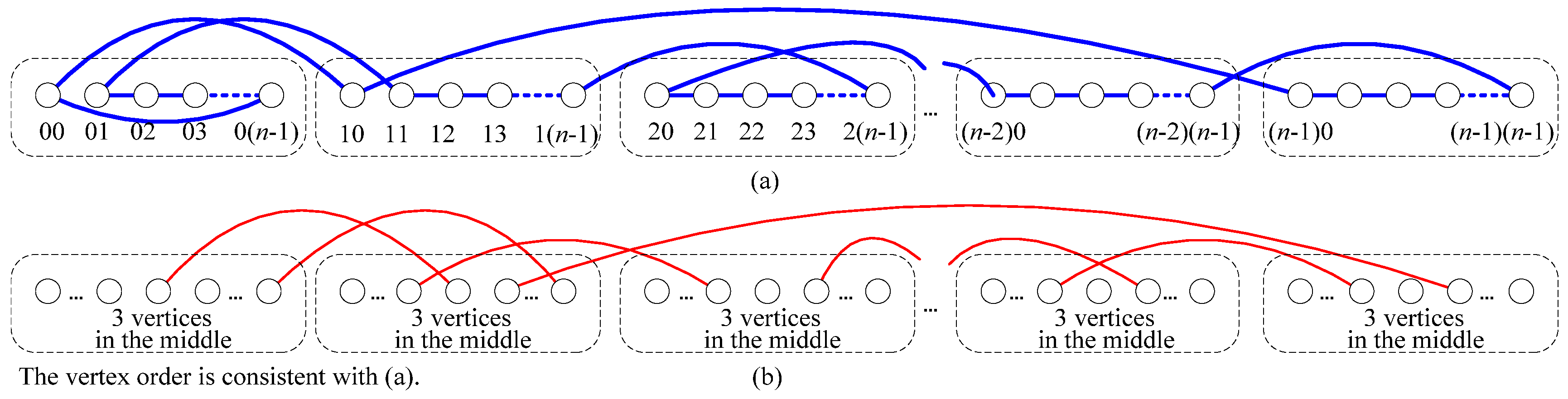Figure 7 is a schematic diagram illustrating the external edges used by two Hamiltonian cycles. Therefore, we can obtain two EDHCs according to Algorithm 2. □

As illustrated in Figure 7, the two Hamiltonian cycles employ distinct pairs of vertices as connection endpoints between BCube(n, 0) components. Specifically, in the first Hamiltonian cycle, the first two vertices are selected as endpoints to connect the first two BCube(n, 0) components, whereas in the second Hamiltonian cycle, the last vertex and a middle vertex serve as the corresponding endpoints. For the connections among the remaining components, the first Hamiltonian cycle uses the first and last vertices as endpoints, while the second Hamiltonian cycle adopts the two middle vertices as endpoints. This endpoint selection guarantees that the two Hamiltonian cycles are edge-disjoint. As an example, when n = 5, two EDHCs can be constructed using Algorithm 2, as shown in Figure 6. The resulting Hamiltonian cycles are (10-00)-04-03-02-(01-11)-12-13-(14-24)-23-22-21-(20-30)-31-32-33-(34-44)-43-42-41-(40-10) and 02-00-03-01-(04-14)-(11-21)-24-22-20-(23-33)-30-32-34-(31-41)-44-42-40-(43-13)-10-(12-02). In the above vertex sequences, the edges enclosed in parentheses denote external edges connecting different BCube(n, 0) components.

According to Lemmas 2, 4, and 5, we have the following theorem.

Theorem 1.

There exist two EDHCs on BCube(n, 1) for n ≥ 3.

Next, we will use BCube(n, 1) as a basis and prove by induction that there exist two EDHCs on BCube(n, k). Similarly, we will provide two lemmas for the cases where n is even and odd.

Lemma 6.

There exist two EDHCs on BCube(n, k) for even n ≥ 4 and k ≥ 1.

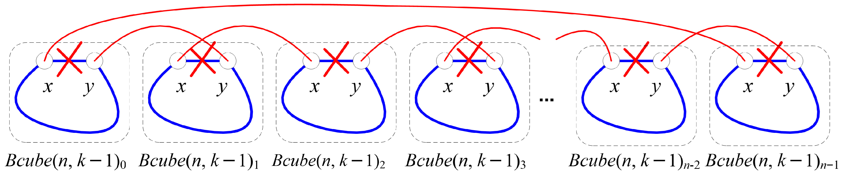
Proof of Lemma

6. A BCube(n, k) is composed of n BCube(n, k − 1), let them be BCube(n, k − 1)₀, BCube(n, k − 1)₁, BCube(n, k − 1)₂, …, BCube(n, k − 1)_n−2, BCube(n, k − 1)_n−1. Select an edge (x, y) in the first Hamiltonian cycle of BCube(n, k − 1)_j and delete it for all j ∈ {0, 1, 2, …, n − 1}.

Next, connect vertex x in BCube(n, k − 1)_j to vertex x in BCube(n, k − 1)_j-1 and connect vertex y in BCube(n, k − 1)_j to vertex y in BCube(n, k − 1)_j+1 while j ∈ {0, 2, 4, …, n − 4, n − 2}. Then, the first Hamiltonian cycle of BCube(n, k) can be obtained, as shown in Figure 8. Similarly, in the second Hamiltonian cycle of BCube(n, k − 1)_j for each j ∈ {0, 1, 2, …, n − 1}, choose an edge (w, z) to delete it where w ≠ x, y and z ≠ x, y. Next, connect vertex w in BCube(n, k − 1)_j to vertex w in BCube(n, k − 1)_j-1 and connect vertex z in BCube(n, k − 1)_j to vertex z in BCube(n, k − 1)_j+1 while j ∈ {0, 2, 4, …, n − 4, n − 2}. Then, the second Hamiltonian cycle of BCube(n, k) can be obtained. Finally, these two Hamiltonian cycles are two EDHCs because there exist two EDHCs in BCube(n, k − 1) and since w ≠ x, y and z ≠ x, y, the external edges connecting BCube(n, k − 1) are edge-disjoint. Therefore, we adopt the two EDHCs generated by Algorithm 1 on BCube(n, 1) as the inductive basis, and this lemma follows by induction. □

Lemma 7.

There exist two EDHCs on BCube(n, k) for odd n ≥ 3 and k ≥ 1.

Proof of Lemma

7. The proof structure is similar to Lemma 6, but since n is odd, the connection between the last two BCube(n, k − 1)s needs to be slightly modified. Select an edge (x, y) in the first Hamiltonian cycle of BCube(n, k − 1)_j and delete it for all j ∈ {0, 1, 2, …, n − 1}. Next, connect vertex x in BCube(n, k − 1)_j to vertex x in BCube(n, k − 1)_j−1 while j ∈ {0, 2, 4, …, n − 5, n − 3}, and connect vertex y in BCube(n, k − 1)_j to vertex y in BCube(n, k − 1)_j+1 while j ∈ {0, 2, 4, …, n − 7, n − 5}. Let z = N(y) and z ≠ x. In last three BCube(n, k − 1), connect y in BCube(n, k − 1)_n−3 to y in BCube(n, k − 1)_n−1, y in BCube(n, k − 1)_n−2 to y in BCube(n, k − 1)_n−1, y in BCube(n, k − 1)_n−2 to x in BCube(n, k − 1)_n−2, z in BCube(n, k − 1)_n−2 to z in BCube(n, k − 1)_n−1 and x in BCube(n, k − 1)_n−1 to x in BCube(n, k − 1)₀. Then, the first Hamiltonian cycle of BCube(n, k) can be obtained, as shown in Figure 9. The construction of the second Hamiltonian cycle of BCube(n, k) is similar to the first one. But we need to select another 3 vertices a, b, c to replace x, y, z and {a, b, c} ∩ {x, y, z} = ∅ to ensure that the two Hamiltonian cycles are edge-disjoint. We show that the required disjoint vertex triples always exist in the inductive step. For n ≥ 3 and k ≥ 1, each BCube(n, k − 1) contains n^k vertices. Since n is odd and n ≥ 3, we have n^k ≥ 9 for all k ≥ 2, and the base case BCube(3, 1) is explicitly handled by Lemma 2. Therefore, after selecting the first triple {x, y, z}, at least n^k − 3 ≥ 6 vertices remain, from which another triple {a, b, c} with {a, b, c} ∩ {x, y, z} = ∅ can always be chosen. This guarantees that the two Hamiltonian cycles constructed in the inductive step are edge-disjoint. Consequently, the construction yields two EDHCs on BCube(n, k), and the lemma follows by induction. □

As shown in Figure 8, when n is even and the number of BCube(n, k − 1) components is also even, all components can be connected straightforwardly by selecting vertices x and y as the connection endpoints. However, when n is odd and the number of BCube(n, k − 1) components is odd, this connection strategy is no longer feasible. To resolve this issue, the last three BCube(n, k − 1) components are treated as a single aggregated component. The Hamiltonian traversal enters this aggregated component through vertex x of BCube(n, k − 1)_n−3, visits all vertices within the three components by means of a Hamiltonian path, and then exits through vertex x of BCube(n, k − 1)_n−1. The schematic illustration of the Hamiltonian-path connections among the last three BCube(n, k − 1) components is provided in Figure 9. By Lemmas 6, 7, and Theorem 1, we have the following theorem.

Theorem 2.

There exist two EDHCs on BCube(n, k) for n ≥ 3 and k ≥ 1.

4. Performance Evaluation

This section presents the simulation of all-to-all broadcasting using two EDHCs as transmission channels in BCube(n, 2), where 3 ≤ n ≤ 9. For performance analysis, the results are compared with those of the conventional method that relies on a single Hamiltonian cycle. To assess efficiency, two broadcast-related metrics are measured, both focused on transmission time (or broadcast latency). Technically, the algorithms for constructing the two EDHCs and along with the simulation program for all-to-all broadcasting, were implemented in C. Experiments were carried out on a system equipped with a 12th-generation Intel^® Core™ i9-12900 CPU, 32 GB RAM (Intel Corporation, Santa Clara, CA, USA) and Linux operating system.

We simulated a scenario in which a message with a size ranging from 1 KB to 3 MB originated from a random source node in the network and was broadcast using two approaches: either a single Hamiltonian cycle or two EDHCs. Taking the standard Ethernet frame as a reference, each frame can carry approximately 1500 bytes of data (excluding the initial preamble, frame delimiter, and the frame check sequence at the end). Consequently, a 3 MB message can be segmented into approximately 3,145,728/1500 ≈ 2097 packets. To evaluate the broadcast efficiency of the two approaches, we conducted 100,000 simulation runs for each. For consistency and fairness, both approaches used the same message script.

The source vertex s of each broadcast is randomly generated from all vertices in the network. Broadcasts are transmitted unidirectionally along a Hamiltonian cycle, ensuring delivery to every node. Since we assume that the message size does not exceed 3 MB, let m be the number of broadcast packets, with m randomly chosen from the range 1 to 2097. For the single Hamiltonian cycle approach, the source vertex s has two adjacent nodes on the cycle. A transmission direction is randomly selected, and during each time slot, the packet is forwarded sequentially along the cycle to the next node. The process continues until the packet returns to the source vertex s, marking the completion of the broadcast. For the two EDHCs approach, both cycles serve as parallel broadcast channels. To balance the load across the two channels, a round-robin scheduling strategy is applied: odd-numbered packets are transmitted along the first cycle, while even-numbered packets are transmitted along the second.

Considering practical network operating conditions, this study assumes that each node on a Hamiltonian cycle not only forwards the packets generated in the simulation to its next node along the cycle, but may also generate and transmit additional background traffic packets to the same next node. All packets must first enter the node’s buffer, where they are queued and wait to be transmitted. To reflect different levels of network load, we introduce a stochastic background traffic model. At each node, packets are generated with a probability determined by the load intensity (LD = 10%, 30%, 50%), corresponding to low, medium, and high loads, respectively. This modeling approach captures the competitive transmission behavior caused by concurrent network activities and enables an evaluation of system performance and stability under varying traffic conditions.

For each vertex v in the network except s and every i with 1 ≤ i ≤ m, let t_v(i) be the transmission time of the i-th packet received by vertex v, measured from the initial transmission. Then the time required for vertex v to receive the entire message can be expressed as ${t\left(v\right)=\mathrm{M}\mathrm{a}\mathrm{x}}_{i=1}^m\left\{t_v\right(i\left)\right\}$. Since we simulated 100,000 broadcast message instances, let msg_j contain m packets and 1 ≤ j ≤ 100,000. Next, two specific metrics called the average transmission time $avg\left({msg}_j\right)=({\sum }_{v\in V\left(G\right)-\left\{s\right\}}{\mathrm{M}\mathrm{a}\mathrm{x}}_{i=1}^m{t}_v\left(i\right))/(\left|V\right(G\left)\right|-1)$ and the maximum transmission time ${max\left({msg}_j\right)={\mathrm{M}\mathrm{a}\mathrm{x}}_{v\in V\left(\mathrm{G}\right)}\{\mathrm{M}\mathrm{a}\mathrm{x}}_{i=1}^m\left\{t_v\left(i\right)\right\}\}$ are defined. Next, we use the following two metrics to evaluate broadcasting efficiency: one is called the average broadcasting latency $ABL={\sum }_{j=1}^{\mathrm{100,000}}avg\left({msg}_j\right)/\mathrm{100,000}$, and the other is called the maximum broadcasting latency $MBL={\mathrm{M}\mathrm{a}\mathrm{x}}_{j=1}^{\mathrm{100,000}}\left\{max\left({msg}_j\right)\right\}$. We conducted simulations on BCube(n, 2) for 3 ≤ n ≤ 9.

Table 2. ABL and MBL using one Hamiltonian cycle for broadcasting in BCube(n, 2) while 3 ≤ n ≤ 9.

BCube(n, 2)	n = 3	n = 4	n = 5	n = 6	n = 7	n = 8	n = 9
ABL(LD = 10%)	1229.00	1286.05	1357.86	1446.78	1550.12	1681.98	1837.43
ABL(LD = 30%)	1587.95	1680.99	1787.41	1910.93	2047.49	2214.99	2405.90
ABL(LD = 50%)	2169.61	2316.26	2465.26	2628.24	2800.71	3007.45	3237.41
MBL(LD = 10%)	2508	2625	2776	2961	3187	3458	3790
MBL(LD = 30%)	3288	3479	3682	3943	4253	4596	5002
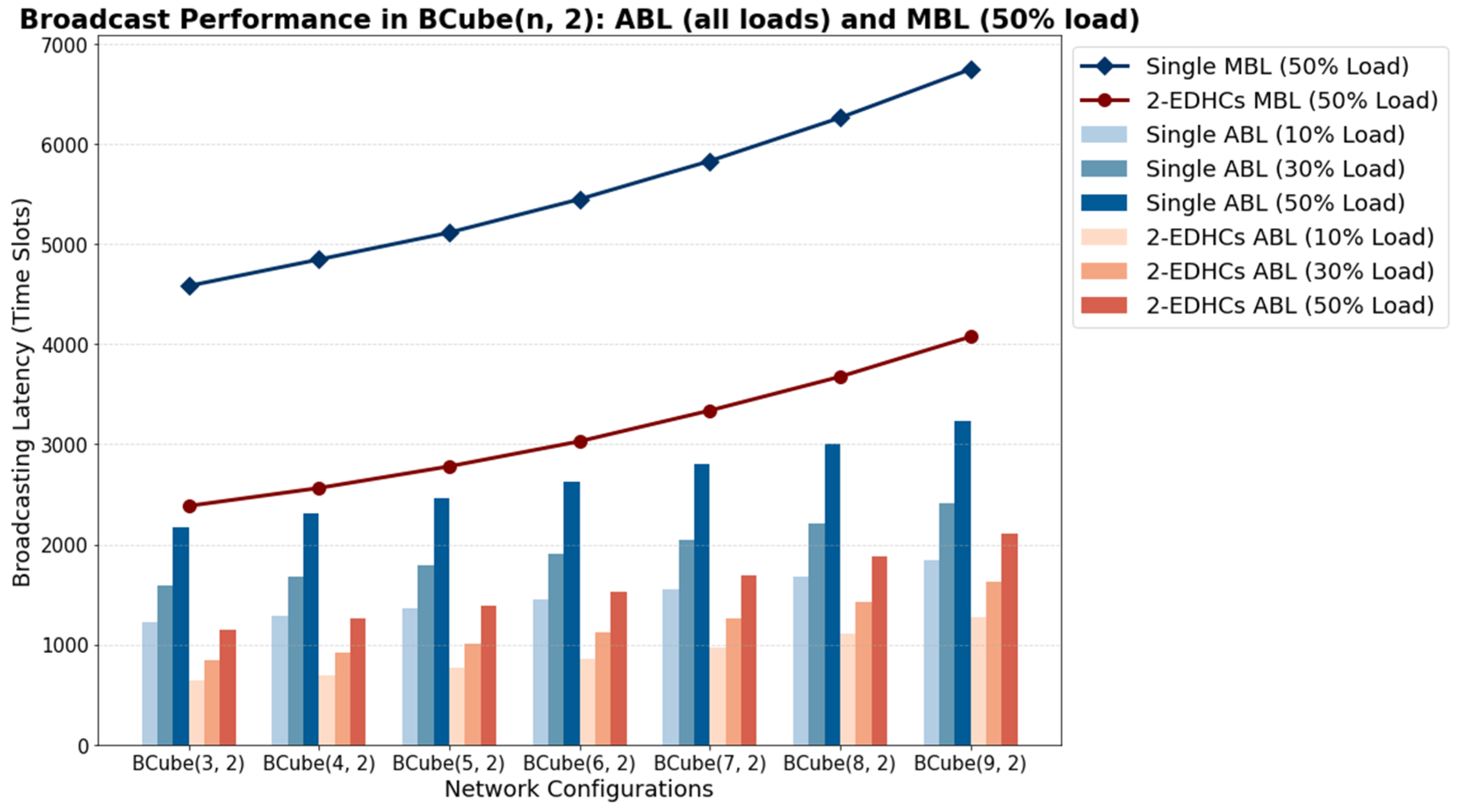
MBL(LD = 40%)	4583	4847	5116	5449	5831	6263	6747

and

Table 3. ABL and MBL using two EDHCs for broadcasting in BCube(n, 2) while 3 ≤ n ≤ 9.

BCube(n, 2)	n = 3	n = 4	n = 5	n = 6	n = 7	n = 8	n = 9
ABL(LD = 10%)	643.76	694.99	768.08	854.49	967.74	1105.55	1278.02
ABL(LD = 30%)	839.14	915.02	1014.72	1125.08	1263.69	1426.71	1623.47
ABL(LD = 50%)	1148.99	1256.04	1386.41	1523.68	1689.40	1881.29	2108.82
MBL(LD = 10%)	1301	1393	1512	1671	1865	2102	2391
MBL(LD = 30%)	1716	1854	2017	2223	2469	2754	3090
MBL(LD = 40%)	2385	2564	2780	3030	3338	3676	4075

report the experimental results for ABL and MBL, corresponding to the approaches using a single Hamiltonian cycle and two EDHCs, respectively.

We combine the data from Table 2 and Table 3 to plot Figure 10, which facilitates comparison of ABL and MBL under two approaches: a single Hamiltonian cycle and two EDHCs.

From Table 2 and Table 3, and Figure 10, we are aware of the following four phenomena:

• For both ABL and MBL, the broadcast delay performance achieved using two EDHCs is superior to that of the traditional approach using a single Hamiltonian cycle. For instance, under a typical load of 30%, the ratio of ABL with two EDHCs to that with one Hamiltonian cycle is approximately 52.9% in BCube(3, 2) (839.14 vs. 1587.95) and about 67.5% in BCube(9, 2) (1623.47 vs. 2405.90). Similarly, the ratio of MBL with two EDHCs to that with one Hamiltonian cycle is around 52.2% in BCube(3, 2) (1716 vs. 3288) and approximately 61.8% in BCube(9, 2) (3090 vs. 5002). More generally, across all evaluated load levels (10%, 30%, and 50%) and network sizes 3 ≤ n ≤ 9, the two EDHCs approach consistently achieves substantially lower ABL and MBL than the single Hamiltonian cycle approach. Although absolute broadcast latencies increase as background traffic intensifies, the relative performance advantage of using two EDHCs remains evident, indicating that exploiting edge-disjoint path parallelism effectively alleviates congestion and improves broadcasting robustness under moderate network load conditions.
• As n increases from 3 to 9 in BCube(n, 2), both ABL and MBL grow steadily under all load conditions. This indicates that broadcasting latency scales with network size due to the increased number of nodes participating in packet forwarding and the accumulation of queuing delays along the Hamiltonian cycles.
• For both one Hamiltonian cycle and two EDHCs approaches, ABL and MBL increase monotonically as the load rises from 10% to 50%. This trend confirms that higher background traffic intensifies buffer contention and transmission competition, leading to longer queuing delays and degraded broadcasting performance.
• As the load increases, the relative performance gap between the single Hamiltonian cycle and two EDHCs approaches becomes more significant. Under high load (50%), the two EDHCs approach achieves lower ABL and MBL, highlighting its stronger robustness and better resistance to background traffic interference in heavy-load network environments.

5. Conclusions

In this paper, we study the construction of two EDHCs on BCube(n, k) for n ≥ 3. Then, we perform broadcast simulations on them and show that using two EDHCs achieves higher transmission efficiency than employing a single Hamiltonian cycle. Before concluding, we note that the reliability and fault tolerance of an interconnection network are fundamentally determined by structural parameters such as node degree, vertex connectivity, and edge connectivity. In the logic graph GH(m_k, m_k−1, …, m₁, m₀) of BCube(n, k), these three parameters coincide and are equal to (n − 1)(k + 1), indicating a highly regular and symmetric topology with strong resistance to both vertex and edge failures. Although such connectivity properties provide an essential foundation for fault-tolerant communication and the construction of disjoint substructures, they are intrinsic to the topology and remain unchanged once the network is fixed. In general, networks with higher edge connectivity can accommodate a larger number of EDHCs, which are important for improving robustness and load balancing. However, the Hamiltonian cycle problem is well known to be NP-complete for general graphs, highlighting the inherent difficulty of establishing Hamiltonicity and, in particular, the existence of multiple EDHCs. Therefore, proving the existence of several EDHCs in BCube(n, k) requires exploiting its specific structural properties rather than relying on general algorithmic techniques. Motivated by the strong degree and connectivity of BCube(n, k), a natural direction for future research is to investigate whether three or even four EDHCs exist in this topology, a question that, to the best of our knowledge, remains open.