Value Matrix Dynamics and Attractor Selection in a Reduced Transformer Model

Abstract

We study an interacting particle system on the unit sphere $S^{d-1}$ motivated by the forward-pass dynamics of a transformer model that combines a value matrix V and a u-aligned multi-layer perceptron (MLP) Φ, a particular form of MLP specified below. For a symmetric value matrix and this MLP, the one-cluster dynamic is the Riemannian gradient flow of an explicit Lyapunov function $L=f_V+g$, which combines the Rayleigh quotient of V with the MLP potential. Every trajectory converges to a fixed point, limit cycles are excluded, and the fixed points are the critical points of L: local maxima are stable attractors and saddles are unstable. Isolating the value matrix ($\mathsf{\Phi }\equiv 0$, with V possibly non-symmetric and a real strictly dominant eigenvalue ${\lambda }_1$), we show that the dominant eigenvector $v_1$ is the selected attractor and that its basin is almost the whole sphere, the two basins of $\pm v_1$ being separated by an invariant subsphere carried by the left eigenvector of V. The subdominant eigenvectors form a hierarchical structure of saddles, and a complex dominant pair replaces the point attractor by a great-circle limit cycle. When the tokens move independently, softmax attention contributes no first-order clustering force: the tokens collapse to $\pm v_1$ at a consensus rate equal to ${\lambda }_1$ and independent of the attention matrix, and whether two clusters in opposite basins coexist or merge is governed by the single order parameter $s=v_1^{\top }A{v}_1$. Thus, the value matrix, rather than the attention, controls the location and the selection of the limiting cluster. All results are confirmed by numerical integration of the continuous-time ordinary differential equation (ODE).

1. Introduction

1.1. Token Dynamics and Interacting Particle Systems

Transformer models [1] process a sequence of tokens through a succession of attention and feed-forward layers. When the layers are regarded as discrete time steps, the forward pass becomes a dynamical system acting on the token representations, and its continuous-time (deep) limit is a system of ordinary differential equations. If the representations are normalised, the tokens evolve as interacting particles on the unit sphere $S^{d-1}$ (in d-dimensional space ${\mathbb{R}}^d$), coupled through the softmax attention weights. This point of view has been developed recently [2,3,4], and reveals that the tokens tend to cluster as the depth increases: the particles aggregate toward a small number of limiting configurations, determined by the initial data and weight matrices. Clustering is the dynamical counterpart of an empirical observation about deep transformers, namely that the token representations tend to become similar to each other, a phenomenon known in the machine learning literature as rank collapse, oversmoothing, or token uniformity [5,6].

The forward pass combines three ingredients: the attention weights, which couple the tokens; the value matrix V, which acts linearly on each token before the attention-weighted sum; and the feed-forward (MLP) block, which acts on each token separately. The question addressed in the present work is how these ingredients interact: which of them selects the limiting cluster, and at what rate the tokens collapse toward it.

1.2. Related Work

The interpretation of self-attention as an interacting particle system on the sphere was introduced by Geshkovski et al. [2,3]. They consider the pure-attention dynamics, in which the value matrix is the identity and no feed-forward block is present, and prove that the tokens cluster in infinite time; the type of limiting configuration depends on the spectrum of the value matrix, and the attention matrix converges to a low-rank Boolean matrix. The mean-field description of these dynamics, in which the empirical measure of the tokens satisfies a nonlinear transport equation, is studied in [4]. These works connect transformer dynamics to classical models of collective behaviour and consensus, such as synchronisation of coupled oscillators [7], self-propelled particle and flocking models [8,9], and opinion dynamics with bounded confidence [10], and to the view of deep residual networks as discretisations of ordinary differential equations [11].

A parallel line of work, motivated by the design of transformer architectures, studies the loss of expressivity caused by clustering. Dong et al. [5] show that pure attention, without skip connections or feed-forward blocks, loses rank doubly exponentially with depth, and that the skip connections and the MLP are precisely what prevents the collapse to a rank-one representation. The role of attention normalisation and layer normalisation in this collapse has been subsequently examined [6], and doubly stochastic variants of attention have been proposed [12]. In all of these works, the value matrix is either the identity or is not the object of study, and the feed-forward block is either absent or treated only qualitatively. Related recent developments include the analysis of clustering under causal attention masking [13], the mean-field study of the perceptron (feed-forward) block, which shows that its critical points are generically atomic and localised on the sphere [14], and the white-box, rate-reduction view of transformer layers [15].

In contrast to these works, which treat the three ingredients of the forward pass (attention, the value matrix, and the feed-forward block) in isolation, the present paper studies their joint action and disentangles their distinct roles: attention drives the collapse, the value matrix selects its location, and the feed-forward block shapes the attractor landscape. The value matrix is added to the model precisely to determine its role in the selection of the limiting cluster.

1.3. Contributions and Outline

We study the token dynamics (1) under two successive simplifications: first, the value matrix acting alone ($\mathsf{\Phi }\equiv 0$), then, the value matrix together with a u-aligned MLP (a particular form of MLP, defined in Section 2). The main results are as follows.

For the value matrix alone, the one-cluster flow $\dot{x}=P_x^{\perp }\left(Vx\right)$ admits a complete and explicit description that requires no symmetry of V. When the dominant eigenvalue ${\lambda }_1$ is real and simple, the corresponding eigenvector $v_1$ is the selected attractor (Theorem 1), and its basin is almost the whole sphere: every trajectory converges to $+v_1$ or $-v_1$ except on a measure-zero invariant subsphere, which is carried by the left eigenvector $w_1$ and is tilted off the geometric equator when V is non-symmetric (Theorem 2, Lemma 4). The subdominant eigenvectors organise into a hierarchical structure of saddles, and a complex dominant pair replaces the point attractor by an invariant great-circle limit cycle (Proposition 1, Remark 6). Whether nearby tokens actually cluster is then governed by the sign of the dominant eigenvalue: ${\lambda }_1>0$ gives collapse to a point, ${\lambda }_1<0$ gives one-cluster stability but token spreading, and a complex dominant pair gives no point cluster at all. Releasing the tokens to move independently under the value matrix, we show that softmax attention contributes no first-order clustering force, so the collapse is governed by V alone. When ${\lambda }_1>0$, the tokens collapse to $\pm v_1$ according to $\mathrm{sign}\langle w_1,x\rangle$, with a consensus rate equal to ${\lambda }_1$ and independent of the attention matrix (Theorem 3), and the positive-eigenvalue hemispheres and cones are trapping (Propositions 2 and 3). Attention cannot override the value matrix: collapse from generic data is robust across all attention classes, and the only genuinely attention-dependent question, whether two clusters in opposite basins coexist or merge, is decided by a single order parameter $s=v_1^{\top }A{v}_1$, the alignment of the attention along the cluster axis, with coexistence for $s>0$ and merging for $s<0$ (Section 4.3).

Adding a u-aligned MLP Φ to a symmetric value matrix V, we show that the combined one-cluster ODE is again a Riemannian gradient flow, now of the explicit Lyapunov function $L=f_V+g$ that combines the Rayleigh quotient of V with the MLP potential g (Theorem 4). Every trajectory converges to a fixed point and limit cycles are excluded; the fixed points are the critical points of L, with local maxima stable and saddles unstable (Corollary 1). Near a stable maximum, the tokens collapse to a single cluster, while near a saddle, the cluster escapes toward the global maximum of L yet remains clustered, under an explicit fluctuation-stability condition (Theorem 5). The dominant eigenvalue of V controls which direction is selected as the global attractor (Remark 11).

These two settings are unified by a general observation, valid for arbitrary V and Φ: a fixed point that is stable for the one-cluster ODE need not be stable for the multi-token system, because the value matrix enters the mean-mode operator but not the fluctuation operator (Proposition 4). The u-aligned MLP with symmetric V is the exactly solvable case in which this instability is structurally excluded. All the analytical results are confirmed by numerical integration of the continuous-time ODE.

The paper is organised as follows. Section 3 treats the value matrix alone in the one-cluster regime: fixed points, the dominant-eigenvector attractor, almost-global bistability, and the hierarchical flag. Section 4 releases the tokens and studies multi-token collapse, trapping, and the role of the attention matrix. Section 5 adds the u-aligned MLP and establishes the Lyapunov structure together with the uncollapsed token dynamics. Section 6 presents the general one-cluster versus multi-token mechanism, and Section 7 is devoted to a discussion of the results.

• Highlights:

• For the value matrix alone, the dominant eigenvector $v_1$ is the selected attractor and its basin is almost the whole sphere; the two basins of $\pm v_1$ are separated by an invariant subsphere carried by the left eigenvector $w_1$, tilted off the geometric equator when V is non-symmetric (Theorems 1 and 2).
• Softmax attention exerts no first-order clustering force (Proposition 5): the collapse rate equals the dominant eigenvalue ${\lambda }_1$ and is independent of the attention matrix, and whether two antipodal clusters coexist or merge is governed by the single order parameter $s=v_1^{\top }A{v}_1$.
• For symmetric V with a u-aligned MLP, the one-cluster flow is the Riemannian gradient flow of $L=f_V+g$; every trajectory converges to a critical point and limit cycles are excluded (Theorem 4).
• One-cluster stability need not imply multi-token stability, because V enters the mean operator $L_{\mathrm{col}}$ but not the fluctuation operator $L_{\mathrm{fluct}}$ (Proposition 4).

2. Model

• Setting

Let n tokens $x_1,\dots ,x_n\in S^{d-1}\subset {\mathbb{R}}^d$ evolve in continuous time. Fix $r\le d$ orthonormal directions $u_1,\dots ,u_r\in S^{d-1}$ and write $s_{ik}=\langle u_k,x_i\rangle$. The continuous-time ODE (the Euler limit of the discrete normalised residual update; cf. the neural-ODE view of residual networks [11]) is:

$${\dot{x}}_i=P_{x_i}^{\perp }\left(\sum _j{w}_{ij}V{x}_j+\mathsf{\Phi }\left(x_i\right)\right),P_x^{\perp }y=y-\langle x,y\rangle x,$$

(1)

where $w_{ij}={\mathrm{softmax}}_j(\beta \langle x_i,A{x}_j\rangle /\sqrt{d})$ are attention weights, A is a coupling matrix, and $\beta >0$. Throughout, $\parallel ·\parallel$ denotes the Euclidean norm on ${\mathbb{R}}^d$ and $\langle ·,·\rangle$ the associated inner product, so $S^{d-1}$ is the unit sphere in this norm.

• Symmetric value matrix

We take $V=V^{\top }$ symmetric with eigenvectors $u_1,\dots ,u_r$ and eigenvalues ${\nu }_1\ge \cdots \ge {\nu }_r\ge 0$. Its Rayleigh quotient is $f_V\left(x\right)={\displaystyle \frac{1}{2}}\langle x,Vx\rangle$. In a full transformer, the attention output is $W_O{\sum }_j{w}_{ij}{W}_V{x}_j$, so the value/output map $V=W_O{W}_V$ acts on the values inside the attention-weighted sum; in the reduced model (1), the same V acts linearly on each token before the attention-weighted average.

• $\mathit{u}$-aligned MLP

We consider a particular form of feed-forward block, in which the input and output directions are tied to the same orthonormal feature basis $\left\{u_k\right\}$. This u-aligned MLP is

$$\mathsf{\Phi }\left(x\right)={\displaystyle \sum _{k=1}^r}{\gamma }_k\sigma ({\alpha }_k{s}_k+b_k)u_k,s_k=\langle u_k,x\rangle ,$$

(2)

where ${\gamma }_k,{\alpha }_k,b_k\in \mathbb{R}$ and σ are continuously differentiable (e.g., tanh). The name refers to this alignment with the basis $\left\{u_k\right\}$, not to coordinatewise action in the standard basis; we avoid the term “diagonal MLP”, which would misleadingly suggest the latter. The same orthonormal directions $u_k$ are used to read each feature $s_k=\langle u_k,x\rangle$ and to write Φ back (tied input/output weights). Each component ${\mathsf{\Phi }}_i\left(x\right)$ therefore depends on all coordinates of x through the $s_k$, so Φ is not coordinatewise in the standard basis; what matters is that its Jacobian,

$$D\mathsf{\Phi }\left(x\right)={\displaystyle \sum _{k=1}^r}{\gamma }_k{\alpha }_k{\sigma }^{\prime }({\alpha }_k{s}_k+b_k)u_k{u}_k^{\top },$$

(3)

is symmetric (diagonal in the u-basis, with eigenvectors $u_k$ and eigenvalues ${\gamma }_k{\alpha }_k{\sigma }^{\prime }({\alpha }_k{s}_k+b_k)$). It is this symmetry, not standard-basis diagonality, that the Lyapunov structure of Section 5 relies on. The associated scalar potential is

$$g\left(x\right)={\displaystyle \sum _{k=1}^r}{\gamma }_k{\int }_0^{s_k}\sigma ({\alpha }_{k}t+b_k)dt.$$

(4)

• Numerical methods

The results below are illustrated by direct numerical integration of the continuous-time system (1) with an explicit Runge–Kutta scheme, and, for the one-cluster map, by the explicit Euler–retraction iteration $x\mapsto (I+hV)x/\parallel (I+hV)x\parallel$; the dimension d, token number n, inverse temperature β, spectrum of V, and step size are stated in each figure caption. Ensembles of initial conditions are drawn uniformly on $S^{d-1}$, and the number of initial conditions behind each reported statistic is given in the corresponding caption (for example, 600 one-cluster initial conditions in Figure 1). Two groups seeded in opposite basins are declared to coexist when their inter-cluster geodesic distance stays bounded away from zero over the integration horizon, and to merge otherwise; this coincides with the sign of the order parameter $s=v_1^{\top }A{v}_1$ of Section 4.3.

3. One Cluster Without MLP

Setting $\mathsf{\Phi }\equiv 0$ isolates the value matrix. The resulting one-cluster flow $\dot{x}=P_x^{\perp }\left(Vx\right)$ admits a sharp, fully explicit analysis that requires no symmetry of V: we locate its fixed points, identify the dominant eigenvector as the selected attractor, show that the selection is almost-global, and organise the remaining dynamics into a hierarchical flag culminating in great-circle limit cycles.

3.1. Fixed Points for the One-Cluster Flow

With $\mathsf{\Phi }\equiv 0$, the one-cluster ODE is

$$\dot{x}=F\left(x\right):=P_x^{\perp }\left(Vx\right)=Vx-\langle x,Vx\rangle x.$$

(5)

Lemma 1

(Fixed points are real eigenvectors). $x^{\ast }\in S^{d-1}$ is a fixed point of (5) iff $V{x}^{\ast }=\lambda x^{\ast }$ for some real λ, necessarily $\lambda =\langle x^{\ast },V{x}^{\ast }\rangle$. In particular, complex eigenvalues of V produce no fixed point on $S^{d-1}$.

Proof. 

$F\left(x^{\ast }\right)=0$ means $V{x}^{\ast }=\langle x^{\ast },V{x}^{\ast }\rangle x^{\ast }$, i.e., $x^{\ast }$ is an eigenvector with eigenvalue $\lambda =\langle x^{\ast },V{x}^{\ast }\rangle \in \mathbb{R}$. Conversely, an eigenvector with real eigenvalue gives $P_{x^{\ast }}^{\perp }\left(V{x}^{\ast }\right)=P_{x^{\ast }}^{\perp }\left(\lambda x^{\ast }\right)=0$. A complex eigenvalue has no real unit eigenvector in ${\mathbb{R}}^d$. □

Lemma 2

(Linearisation). At a fixed point $x^{\ast }=v_k$ with $V{v}_k={\lambda }_k{v}_k$, the linearisation of (5) on $T_{v_k}{S}^{d-1}$ is

$$A_k:=P_{v_k}^{\perp }V{|}_{T_{v_k}{S}^{d-1}}-{\lambda }_{k}I,$$

(6)

and its spectrum is $\{{\lambda }_j-{\lambda }_k:j\ne k\}$, where ${\lambda }_1,\dots ,{\lambda }_d$ are the eigenvalues of V. This holds for arbitrary (possibly non-symmetric) V.

Proof. 

Differentiating $F\left(x\right)=Vx-\left(x^{\top }Vx\right)x$ at $x=v_k$ in a direction $\xi \in T_{v_k}{S}^{d-1}$ (so $\langle v_k,\xi \rangle =0$) gives:

$$DF\left(v_k\right)\xi =V\xi -\left({\xi }^{\top }V{v}_k+v_k^{\top }V\xi \right)v_k-\left(v_k^{\top }V{v}_k\right)\xi .$$

Now, ${\xi }^{\top }V{v}_k={\lambda }_k\langle \xi ,v_k\rangle =0$, and $v_k^{\top }V{v}_k={\lambda }_k$. The remaining inner term $\left(v_k^{\top }V\xi \right)v_k=\langle V^{\top }{v}_k,\xi \rangle v_k$ is parallel to $v_k$, hence normal to $T_{v_k}{S}^{d-1}$; the tangential generator is its projection,

$$A_k\xi =P_{v_k}^{\perp }\left(DF\left(v_k\right)\xi \right)=P_{v_k}^{\perp }V\xi -{\lambda }_k\xi ,$$

which is (6); the asymmetric part of V drops out through $P_{v_k}^{\perp }$. For the spectrum, complete $v_k$ to an orthonormal basis $\{v_k,q_2,\dots ,q_d\}$ of ${\mathbb{R}}^d$, where $q_2,\dots ,q_d$ is an arbitrary orthonormal basis of $v_k^{\perp }$ (not eigenvectors of V which, V being non-symmetric, need be neither orthogonal nor real). Block-triangularity below uses only that $v_k$ is an eigenvector. Write $J=\left[q_2\right|\cdots \left|q_d\right]$ for the tangent block (so $J^{\top }J=I$, $J^{\top }{v}_k=0$ and $J{J}^{\top }=P_{v_k}^{\perp }$) and $Q=\left[v_k\right|J]$ (orthogonal); using $V{v}_k={\lambda }_k{v}_k$, the similarity $\tilde{V}=Q^{\top }VQ$ has first column ${({\lambda }_k,0,\dots ,0)}^{\top }$, hence

$$\tilde{V}=\left(\begin{array}{cc}{\lambda }_k& b^{\top }\\ 0& M\end{array}\right),\det (\tilde{V}-sI)=({\lambda }_k-s)\det (M-sI),$$

with $b\in {\mathbb{R}}^{d-1}$ generally nonzero (the asymmetry, lying in the normal direction) and $M=J^{\top }VJ$ the lower-right block. Thus, $\mathrm{spec}\left(M\right)=\mathrm{spec}\left(V\right)\setminus \left\{{\lambda }_k\right\}={\left\{{\lambda }_j\right\}}_{j\ne k}$, read off the characteristic polynomial without diagonalising M. Finally, $M=J^{\top }VJ$ is exactly the matrix of the compression $P_{v_k}^{\perp }{V|}_T$ in the basis $\left\{q_m\right\}$: for $q_l,q_m\in T$,

$$\langle q_l,P_{v_k}^{\perp }V{q}_m\rangle =\langle P_{v_k}^{\perp }{q}_l,V{q}_m\rangle =\langle q_l,V{q}_m\rangle ={\left(J^{\top }VJ\right)}_{lm},$$

using $P_{v_k}^{\perp }{q}_l=q_l$ for $q_l\in T$ (the off-diagonal $b^{\top }=v_k^{\top }VJ$ is the discarded normal component). Hence, $A_k=M-{\lambda }_{k}I$ and $\mathrm{spec}\left(A_k\right)=\mathrm{spec}\left(M\right)-{\lambda }_k={\{{\lambda }_j-{\lambda }_k\}}_{j\ne k}$. □

A single observation underlies the global picture of the next subsections: the flow is the radial projection of a linear flow.

Lemma 3

(Projectivised flow). For any $y_0\ne 0$, let $y\left(t\right)=e^{tV}{y}_0$ and $x\left(t\right)=y\left(t\right)/\parallel y\left(t\right)\parallel$. Then, $x\left(t\right)$ solves $\dot{x}=P_x^{\perp }\left(Vx\right)$, and conversely, every solution of the latter is the radial projection of a ray of $\dot{y}=Vy$.

Proof. 

Differentiating $x=y/\parallel y\parallel$ and using $\dot{y}=Vy$ and $\frac{d}{dt}\parallel y\parallel =\langle y,Vy\rangle /\parallel y\parallel$,

$$\dot{x}={\displaystyle \frac{Vy}{\parallel y\parallel }}-{\displaystyle \frac{y\langle y,Vy\rangle }{{\parallel y\parallel }^3}}=Vx-\langle x,Vx\rangle x=P_x^{\perp }\left(Vx\right).$$

Conversely, given a solution $x\left(t\right)$ on $S^{d-1}$, the scalar ODE $\frac{d}{dt}\rho =\langle x,Vx\rangle \rho$ reconstructs $\parallel y\parallel =\rho$, and $y=\rho x$ solves $\dot{y}=Vy$. □

Lemmas 1–3 are elementary and classical. Lemma 3 exhibits the one-cluster flow as the radial projection (projectivisation) of the linear flow $e^{tV}$, and the convergence of that projection to the dominant eigendirection is the continuous-time counterpart of the power method [16]. We include self-contained proofs for completeness; the contribution of this section is not these lemmas individually but their assembly into the almost-global attractor-selection picture, the left-eigenvector separator, and the hierarchical flag developed in the following subsections.

3.2. The Dominant-Eigenvector Attractor

Theorem 1

(One-cluster attractor). Suppose ${\lambda }_1\in \mathbb{R}$ is a simple eigenvalue of V with a strictly maximal real part, ${\lambda }_1>\mathrm{Re}{\lambda }_j$ for every other eigenvalue ${\lambda }_j$ of V, and let $v_1$ be the corresponding unit eigenvector. Then, $v_1$ is locally asymptotically stable for (5). Every other real eigenvector $v_k$ ($k\ne 1$) is unstable, with unstable dimensions equal to the number of $\{j:\mathrm{Re}{\lambda }_j>{\lambda }_k\}\ge 1$.

Proof. 

By Lemma 2, $\mathrm{spec}\left(A_1\right)={\{{\lambda }_j-{\lambda }_1\}}_{j\ne 1}$. Strict dominance gives $\mathrm{Re}({\lambda }_j-{\lambda }_1)=\mathrm{Re}{\lambda }_j-{\lambda }_1<0$ for every $j\ne 1$, so $A_1$ is a possibly non-normal matrix with eigenvalues with negative real parts, and $v_1$ is locally asymptotically stable; non-normality permits transient growth but not loss of asymptotic stability. At any other real eigenvector $v_k$, $\mathrm{spec}\left(A_k\right)={\{{\lambda }_j-{\lambda }_k\}}_{j\ne k}$ contains ${\lambda }_1-{\lambda }_k>0$ (and more generally one positive-real eigenvalue for each ${\lambda }_j$ with $\mathrm{Re}{\lambda }_j>{\lambda }_k$), so $v_k$ is unstable with the stated index. □

Remark 1

(Complex dominant eigenvalue ⇒ no point attractor). If the eigenvalue of the maximal real part is a complex pair, no real eigenvector carries it, so by Theorem 1, every real-eigenvector fixed point has at least one unstable direction and none are stable. On $S^2$ this forces, by the Poincaré–Bendixson theorem, a periodic orbit; this is the limit-cycle mechanism of the asymmetric-V analysis. The clean statement that the top eigenvalue is the unique attractor is thus exactly the real-dominant-eigenvalue case.

3.3. Almost-Global Bistability and the Tilted Separator

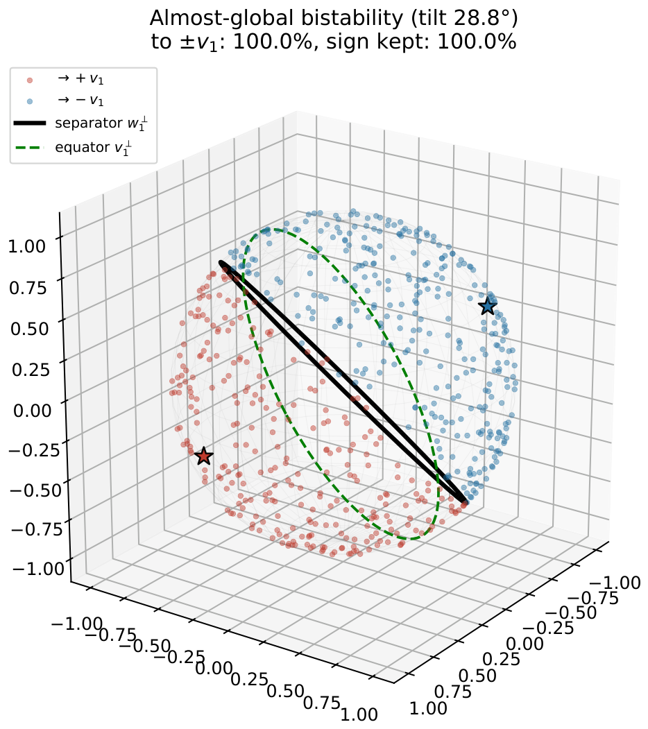
Informally, almost-global bistability states that, outside a measure-zero set of initial data, every trajectory ends at one of the two poles $\pm v_1$. The reason is transparent from the projectivised-flow viewpoint of Lemma 3: writing $x_0={\sum }_k{c}_k{v}_k$ in the eigenbasis, the solution is $x\left(t\right)=e^{tV}{x}_0/\parallel e^{tV}{x}_0\parallel$, and the dominant mode $c_1{e}^{{\lambda }_{1}t}{v}_1$ outgrows all others whenever $c_1\ne 0$, so the limit is determined by the sign of $c_1=\langle w_1,x_0\rangle$ alone. The exceptional set is exactly $\{c_1=0\}=w_1^{\perp }\cap S^{d-1}$, a great subsphere of one lower dimension. Two features are specific to a non-symmetric V: the selector is the left eigenvector $w_1$, so the separating subsphere is $w_1^{\perp }$ rather than the geometric equator $v_1^{\perp }$, and is tilted off it; further, the sign of $\langle w_1,x\rangle$ is exactly conserved along the flow, so the two basins never mix. The following lemma and theorem make this precise.

Lemma 4

(Invariant separating sphere). Let $w_1$ be the left eigenvector of V for ${\lambda }_1$ ($V^{\top }{w}_1={\lambda }_1{w}_1$). Along any solution of (5),

$${\displaystyle \frac{d}{dt}}\langle w_1,x\rangle =\left({\lambda }_1-\langle x,Vx\rangle \right)\langle w_1,x\rangle .$$

(7)

Hence, $\langle w_1,x\left(t\right)\rangle =\langle w_1,x_0\rangle \exp {\int }_0^t\left({\lambda }_1-\langle x\left(s\right),Vx\left(s\right)\rangle \right)ds$; the sign of $\langle w_1,x\rangle$ is conserved, and the great subsphere $H=\{x\in S^{d-1}:\langle w_1,x\rangle =0\}=w_1^{\perp }\cap S^{d-1}$ is invariant.

Proof. 

Using $P_x^{\perp }\left(Vx\right)=Vx-\langle x,Vx\rangle x$ and $\langle w_1,Vx\rangle =\langle V^{\top }{w}_1,x\rangle ={\lambda }_1\langle w_1,x\rangle$,

$${\displaystyle \frac{d}{dt}}\langle w_1,x\rangle =\langle w_1,P_x^{\perp }\left(Vx\right)\rangle =\langle w_1,Vx\rangle -\langle x,Vx\rangle \langle w_1,x\rangle =\left({\lambda }_1-\langle x,Vx\rangle \right)\langle w_1,x\rangle ,$$

which is (7). The integrating factor is positive, so $\langle w_1,x\rangle$ never changes sign, and $\langle w_1,x_0\rangle =0$ forces $\langle w_1,x\rangle \equiv 0$. □

The use of the left eigenvector is essential: it is $w_1^{\top }$, not $v_1^{\top }$, that satisfies $w_1^{\top }V={\lambda }_1{w}_1^{\top }$, so only the coordinate $\langle w_1,x\rangle$ decouples. By biorthogonality $\langle w_1,v_k\rangle ={\delta }_{1k}$, the invariant subspace $w_1^{\perp }$ equals $\mathrm{span}\{v_2,\dots ,v_d\}$ (the complement of $v_1$ in the eigenbasis), not the geometric complement $v_1^{\perp }$; the two agree if $V=V^{\top }$.

Theorem 2

(Almost-global bistability). Under the hypotheses of Theorem 1, assume V is diagonalisable (Remark 3 removes this) and normalise $\langle w_1,v_1\rangle =1$. Then $\pm v_1$ are asymptotically stable, and for every $x_0$ with $\langle w_1,x_0\rangle \ne 0$, the ω-limit set is the single point $\omega \left(x_0\right)=\left\{\mathrm{sign}\langle w_1,x_0\rangle v_1\right\}$. The basins are the open half-spheres $W^{\pm }=\{\pm \langle w_1,x\rangle >0\}$, which exhaust $S^{d-1}\setminus H$; their common boundary is the invariant subsphere H, which contains every fixed point other than $\pm v_1$ together with all of their stable manifolds, and has an empty interior. No globally attracting point exists.

Proof. 

Write $y_0={\sum }_k{c}_k{v}_k$ in the (right) eigenbasis, with $c_1=\langle w_1,y_0\rangle$ by biorthogonality. By Lemma 3, $x\left(t\right)=e^{tV}{y}_0/\parallel e^{tV}{y}_0\parallel$. If $c_1\ne 0$,

$$e^{-{\lambda }_{1}t}{e}^{tV}{y}_0=c_1{v}_1+\sum _{k\ne 1}{e}^{({\lambda }_k-{\lambda }_1)t}(\cdots )\underset{t\to \infty }{\to }{c}_1{v}_1,$$

since every other mode carries a factor $e^{(\mathrm{Re}{\lambda }_k-{\lambda }_1)t}\to 0$ (the imaginary parts only rotate the shrinking components; the approach may spiral but $\mathrm{dist}(x\left(t\right),\pm v_1)\to 0$). Since $e^{-{\lambda }_{1}t}>0$ is a scalar and normalisation is scale-invariant, we may insert this factor in both numerator and denominator without changing $x\left(t\right)$:

$$x\left(t\right)={\displaystyle \frac{e^{tV}{y}_0}{\parallel e^{tV}{y}_0\parallel }}={\displaystyle \frac{e^{-{\lambda }_{1}t}{e}^{tV}{y}_0}{\parallel e^{-{\lambda }_{1}t}{e}^{tV}{y}_0\parallel }}\underset{t\to \infty }{\to }{\displaystyle \frac{c_1{v}_1}{\parallel c_1{v}_1\parallel }}=\mathrm{sign}\left(c_1\right)v_1,$$

the magnitude $|c_1|$ cancelling so that only the sign of the (real) dominant coefficient survives. Hence $\omega \left(x_0\right)=\left\{\mathrm{sign}\left(c_1\right)v_1\right\}$, with $\mathrm{sign}\left(c_1\right)=\mathrm{sign}\langle w_1,x_0\rangle$ constant by Lemma 4. In particular, no $x_0$ off H can lie on the stable manifold of any other fixed point: such a fixed point is a real eigenvector $v_k$ ($k\ge 2$) with $\langle w_1,v_k\rangle =0$, and convergence to it would require $c_1\to 0$, impossible when $c_1\ne 0$ is conserved in sign. All other fixed points and their stable manifolds therefore lie in $H=\{\langle w_1,x\rangle =0\}$; concretely, they form the heteroclinic skeleton of the deflated dynamics on H (Remark below). Local asymptotic stability of $\pm v_1$ is Theorem 1; oddness of $P_x^{\perp }\left(Vx\right)$ gives two disjoint basins, neither the whole sphere, ruling out a global attractor. □

Remark 2

(Mode of approach). Convergence to the point $v_1$ ($\mathrm{dist}(x\left(t\right),v_1)\to 0$) need not be monotone: when the subdominant eigenvalues are complex, the trajectory spirals into $v_1$, winding infinitely while the distance decays like $e^{-({\lambda }_1-\mathrm{Re}{\lambda }_2)t}$. This is still $\omega \left(x_0\right)=\left\{v_1\right\}$.

Remark 3

(Non-diagonalisable V). The diagonalisability hypothesis is only a convenience. If some subdominant eigenvalue is defective, $e^{tV}$ carries Jordan terms $t^m{e}^{{\lambda }_{k}t}$, but since $\mathrm{Re}{\lambda }_k<{\lambda }_1$ strictly we still have $t^m{e}^{({\lambda }_k-{\lambda }_1)t}\to 0$, so $e^{-{\lambda }_{1}t}{e}^{tV}{y}_0\to \left(\mathit{projection}\mathit{of}{y}_0\mathit{onto}\mathit{the}{\lambda }_1\text{-}\mathit{eigenline}\right)$ and Theorem 2 hold verbatim, with $\langle w_1,x_0\rangle$ the coordinate read off by the left eigenvector. Only ${\lambda }_1$ itself must be simple.

Remark 4

(Phase portrait and the separating sphere). On $H=w_1^{\perp }\cap S^{d-1}$ the flow is, by Lemma 3, the projectivisation of $\dot{y}=Vy$ restricted to the invariant subspace $w_1^{\perp }$, on which V acts as the deflated block M with spectrum ${\left\{{\lambda }_j\right\}}_{j\ne 1}$ (Lemma 2). Thus, the dynamics on $H\cong S^{d-2}$ are the same problem one dimension down, and the structure of the basin boundary follows by recursion on the subdominant spectrum:

• If the eigenvalue of M of the maximal real part is real and strictly dominant, H carries its own antipodal pair of attractors, and the remaining real eigenvectors are lower equatorial saddles (their indices given by deflation), forming a heteroclinic skeleton;
• If it is a complex pair, H has no equatorial point at its top; for $d=3$ (so $H\cong S^1$), Poincaré–Bendixson forces H to be a single periodic orbit, a limit cycle bounding the two basins.

For non-symmetric V, the subdominant right eigenvectors $v_k$ ($k\ge 2$) need not lie on the geometric equator; relative to $w_1$ they sit at $\langle w_1,v_k\rangle =0$, hence on H, so they are exactly the equatorial unstable fixed points.

Remark 5

(Discrete-time threshold). The distinction is between the real part and the modulus: the ODE selects the eigenvalue of the largest real part, whereas the discrete map, being power iteration, selects the eigenvalue of the largest modulus $|1+h\lambda |$. These two orderings can disagree at finite step h, and the threshold below is exactly where they do. 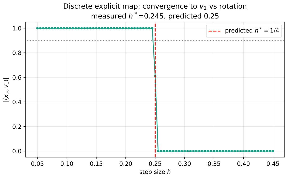The explicit Euler–retraction scheme $x_{i+1}=(I+hV)x_i/\parallel (I+hV)x_i\parallel$ is power iteration for $I+hV$, and converges to the eigenvector of maximal modulus $|1+h{\lambda }_k|$. Since ${|1+h\lambda |}^2=1+2h\mathrm{Re}\lambda +h^2{\left|\lambda \right|}^2$,

$$\log |1+h\lambda |=h\mathrm{Re}\lambda +\frac{h^2}{2}\left({\left(\mathrm{Im}\lambda \right)}^2-{\left(\mathrm{Re}\lambda \right)}^2\right)+O\left(h^3\right),$$

so the leading $O\left(h\right)$ term reproduces the ODE Lyapunov exponent $\mathrm{Re}\lambda$, while the $O\left(h^2\right)$ correction adds a spurious $+\frac{h^2}{2}{\left(\mathrm{Im}\lambda \right)}^2$ favouring rotation. A subdominant complex pair can therefore win the modulus competition at finite step. For $\mathrm{spec}\left(V\right)=\{1,\pm 3i\}$, $|1+h|>|1\pm 3hi|\iff {(1+h)}^2>1+9h^2\iff h<\frac{1}{4}$, so the discrete map converges to $v_1$ only for $h<\frac{1}{4}$ and otherwise rotates (Figure 2). As $h\to 0$, the real-part ordering is restored, recovering the ODE result of Theorem 2; in numerics, $dt$ must stay below this threshold.

3.4. Complex Dominant Pair: Great-Circle Limit Cycle and the Hierarchical Flag

In decreasing dimensions, the attractor and its separating sphere is the same problem one dimension down. Order the eigenvalues of V by strictly descending the real part and group them into blocks $B_1,\dots ,B_p$, each a single real eigenvalue (real eigenline $E_j$, $\dim 1$) or a single complex-conjugate pair (real invariant plane $E_j=\mathrm{span}\{\mathrm{Re}{v}_j,\mathrm{Im}{v}_j\}$, $\dim 2$), with $\mathrm{Re}\left(B_1\right)>\cdots >\mathrm{Re}\left(B_p\right)$. Let $W_m=E_1\oplus \cdots \oplus E_m$ collect the m fastest blocks and $F_m=E_{m+1}\oplus \cdots \oplus E_p$ its V-invariant complement; by biorthogonality, $F_m$ is the joint kernel of the left eigen-functionals of $B_1,\dots ,B_m$. Set $H_m=F_m\cap S^{d-1}$, $H_0=S^{d-1}$.

Proposition 1

(Flag of invariant subspheres). For V diagonalisable with strictly separated real block parts, the $H_m$ form an invariant flag

$$S^{d-1}=H_0\supset H_1\supset \cdots \supset H_{p-1}\supset H_p=⌀,{\mathrm{codim}}_{H_{m-1}}{H}_m=\dim E_m\in \{1,2\},$$

and the flow restricted to $H_{m-1}$ has a unique attractor $A_m$:

• If $B_m$ is real, $A_m=\{\pm v_m\}$, an antipodal pair of fixed points;
• If $B_m$ is a complex pair ${\alpha }_m\pm i{\beta }_m$, $A_m=E_m\cap S^{d-1}$ is a great circle: a single periodic orbit of period $2\pi /|{\beta }_m|$ (uniform rotation when $E_m$ is orthonormal, a reparameterisation otherwise).

The basin of $A_m$ within $H_{m-1}$ is the open dense stratum $H_{m-1}\setminus H_m$; $A_m$ is normally hyperbolic with transverse contraction governed by the real-part gap ${\alpha }_m-\mathrm{Re}\left(B_{m+1}\right)>0$, and its unstable dimension equals the depth $\dim W_{m-1}={\sum }_{j<m}\dim E_j$. The strata ${\{H_{m-1}\setminus H_m\}}_{m=1}^p$ partition $S^{d-1}$ into nested basins (an “onion”), each flowing to its $A_m$.

Proof. 

$F_m$ is V-invariant, so $H_m$ is invariant (Lemma 3), and the left-functional description of $F_m$ together with Lemma 4 gives the sign-preservation nesting the strata. On $H_{m-1}$, the dominant surviving block is $B_m$, strictly dominant in the real part, so $e^{-\mathrm{Re}\left(B_m\right)t}{e}^{tV}{y}_0$ converges to the $E_m$-component of $y_0$ (the argument of Theorem 2 applied to ${V|}_{F_{m-1}}$): a point $\pm v_m$ if $B_m$ is real, the rotating $E_m$-component if complex, whose projectivisation is the great circle. The index is the deflation count of faster blocks; normal hyperbolicity follows from the spectral gaps. □

Remark 6

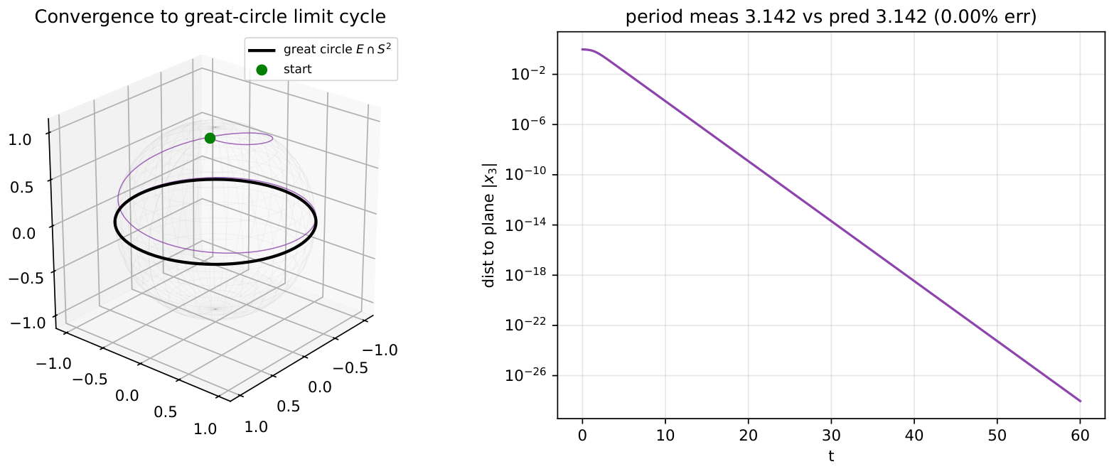
(Limit cycles are exact great circles, not Hopf cycles). The periodic orbits $A_m=E_m\cap S^{d-1}$ are exact invariant great circles, present for every V carrying the pair, at full amplitude and with rotation number fixed by ${\beta }_m=\left|\mathrm{Im}{\lambda }_m\right|$ (Figure 3). They are not small-amplitude cycles born from a Hopf bifurcation: there is no amplitude parameter to grow, since the circle is the projectivisation of the V-invariant eigenplane and is one-dimensional by construction at all parameter values. What does vary is the circle’s stability, set entirely by where $\mathrm{Re}{\lambda }_m$ sits in the real-part order—$A_m$ is the level-m attractor when $B_m$ is the dominant survivor, and a saddle or in-plane repeller otherwise. A “bifurcation” is thus an exchange of dominance (the global attractor switching between a point-pair and a circle as two real parts cross), not the nucleation of a cycle from a fixed point. Two complex pairs with equal real parts are the degenerate exception: their joint four-plane projectivises to an invariant $S^3$ with a two-frequency linear flow (invariant tori); strict separation excludes this.

Remark 7

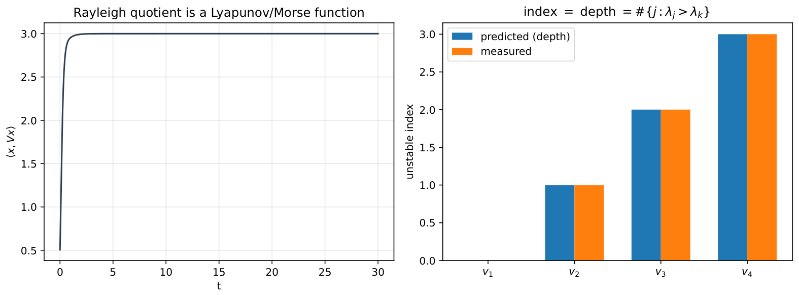
(The symmetric case). When $V=V^{\top }$ all blocks are real, every $A_m$ is a point-pair, the eigenvectors are orthogonal ($w_m=v_m$), and the flow is the gradient ascent of the Rayleigh quotient $f\left(x\right)=\frac{1}{2}\langle x,Vx\rangle$: a Morse function on $S^{d-1}$ with critical pairs $\pm v_k$, values $\frac{1}{2}{\lambda }_k$, and Morse index = depth equals the number of $\{j:{\lambda }_j>{\lambda }_k\}$ (Figure 4). The onion is the orthogonal nested-equator decomposition. For non-symmetric V, the gradient/Morse structure is lost exactly when a complex block appears: $A_m$ becomes a Morse–Bott circle carrying rotation and f ceases to be monotone, but the inclusions and the index-by-depth bookkeeping survive unchanged.

4. Multi-Token, No MLP

Section 3 followed a single cluster. We now release the n tokens to move independently under the value matrix ($\mathsf{\Phi }\equiv 0$). Softmax attention couples them through configuration-dependent convex means, but cannot override V: when ${\lambda }_1>0$, the tokens collapse to $\pm v_1$ with an attention-independent consensus rate, positive hemispheres and cones are trapping, and the one genuinely attention-dependent question, whether two antipodal clusters coexist, is decided by the single scalar $s=v_1^{\top }A{v}_1$. We use the terminology consistently: clustering (equivalently, collapse) means convergence of the tokens to a common point of $S^{d-1}$, whereas spreading means growth of the inter-token fluctuations; the two are governed, respectively, by the operators $L_{\mathrm{col}}$ and $L_{\mathrm{fluct}}$ introduced in Section 6.

4.1. Collapse to the Dominant Eigenvector

Theorem 3

(Multi-token attractor, conditional). Under the hypotheses of Theorem 1, consider the n-token system ${\dot{x}}_i=P_{x_i}^{\perp }{\sum }_j{w}_{ij}V{x}_j$ near the collapsed state $x_i=v_1$. The linearised dynamics split into:

• A mean mode $\dot{\overline{\xi }}=(P_{v_1}^{\perp }V{P}_{v_1}^{\perp }-{\lambda }_{1}I)\overline{\xi }=L_{\mathrm{col}}\overline{\xi }$, with spectrum ${\{{\lambda }_j-{\lambda }_1\}}_{j\ne 1}$ (stable, by Lemma 2);
• Fluctuation modes ${\dot{\zeta }}_i=L_{\mathrm{fluct}}{\zeta }_i$, with $L_{\mathrm{fluct}}=-{\lambda }_{1}I$.

Consequently, if ${\lambda }_1>0$ the fluctuations decay at rate ${\lambda }_1$ and the tokens collapse to $v_1$, which is an attractor of the full system; if ${\lambda }_1<0$, the fluctuations grow and the tokens spread while the mean remains at $v_1$.

Proof. 

Write $x_i=v_1+{\xi }_i$, ${\xi }_i\in T_{v_1}{S}^{d-1}$, and split ${\xi }_i=\overline{\xi }+{\zeta }_i$ into mean and fluctuation ($\overline{\xi }=\frac{1}{n}{\sum }_i{\xi }_i$, ${\sum }_i{\zeta }_i=0$). Since $\mathsf{\Phi }\equiv 0$, the force is $S_i={\sum }_j{w}_{ij}V{x}_j$. At first order, the attention weights satisfy ${\sum }_j{w}_{ij}V{x}_j=V{v}_1+V\overline{\xi }+{O(\parallel \xi \parallel }^2)$: writing $w_{ij}=\frac{1}{n}+O(\parallel \xi \parallel )$, the $O(\parallel \xi \parallel )$ correction to the weights multiplies $V{v}_1$ (an i-independent vector) and sums to zero after using ${\sum }_j$ (correction)$=0$, while the $\frac{1}{n}$ part of the weights gives $\frac{1}{n}{\sum }_{j}V(v_1+{\xi }_j)=V{v}_1+V\overline{\xi }$; the fluctuations ${\zeta }_j={\xi }_j-\overline{\xi }$ do not survive this averaging since ${\sum }_j{\zeta }_j=0$. Hence, $S_i={\lambda }_1{v}_1+V\overline{\xi }+{O(\parallel \xi \parallel }^2)$, independent of i to this order.

Expanding ${\dot{x}}_i=P_{x_i}^{\perp }{S}_i$ exactly as in the proof of Lemma 2 (replacing $Vx$ there by the common force $S_i$, using $P_{v_1}^{\perp }\left({\lambda }_1{v}_1\right)=0$ and $\langle v_1,{\xi }_i\rangle =0$) yields:

$${\dot{\xi }}_i=P_{v_1}^{\perp }\left(V\overline{\xi }\right)-{\lambda }_1{\xi }_i+{O(\parallel \xi \parallel }^2).$$

Averaging over i gives the mean equation $\dot{\overline{\xi }}=(P_{v_1}^{\perp }V{P}_{v_1}^{\perp }-{\lambda }_{1}I)\overline{\xi }=L_{\mathrm{col}}\overline{\xi }$, with spectrum ${\{{\lambda }_j-{\lambda }_1\}}_{j\ne 1}$ by Lemma 2, hence stable. Subtracting the mean equation from the ${\xi }_i$ equation, the $P_{v_1}^{\perp }\left(V\overline{\xi }\right)$ term cancels (it is i-independent) and only the curvature term survives:

$${\dot{\zeta }}_i=-{\lambda }_1{\zeta }_i+{O(\parallel \xi \parallel }^2)=:L_{\mathrm{fluct}}{\zeta }_i,L_{\mathrm{fluct}}=-{\lambda }_{1}I.$$

The sign of ${\lambda }_1$ decides collapse versus spreading. □

Remark 8

(Relation to the general mechanism). Theorem 3 is the MLP-free instance of Proposition 4. Collapse needs ${\lambda }_1>0$, the special case of $\eta >0$ with $\eta ={\lambda }_1>0$ (for V with ${\lambda }_1>0$ and $V⪰0$ on the tangent space). The spreading regime ${\lambda }_1<0$ (a negative dominant eigenvalue) is the MLP-free realisation of Proposition 4(ii): one-cluster stable, multi-token unstable.

4.2. Trapping and Drain

Throughout this subsection, $\mathsf{\Phi }\equiv 0$ and we write the n-token system as

$${\dot{x}}_i=P_{x_i}^{\perp }{S}_i,S_i:=\sum _j{w}_{ij}V{x}_j,{\rho }_i:=\langle x_i,S_i\rangle ,$$

(8)

with $W=\left(w_{ij}\right)$, the row-stochastic attention matrix ($w_{ij}>0$, ${\sum }_j{w}_{ij}=1$), and $D_{\rho }=\mathrm{diag}({\rho }_1,\dots ,{\rho }_n)$. Both W and $D_{\rho }$ depend on $x_i$; no claim below assumes them constant.

• The left-eigenvector reduction

Lemma 5

(Scalar reduction). Let $w_k$ be a left eigenvector of V, $V^{\top }{w}_k={\lambda }_k{w}_k$, and set $p_i^{\left(k\right)}:=\langle w_k,x_i\rangle$, $p^{\left(k\right)}={(p_1^{\left(k\right)},\dots ,p_n^{\left(k\right)})}^{\top }$. Then, along (8),

$${\dot{p}}_i^{\left(k\right)}={\lambda }_k\sum _j{w}_{ij}{p}_j^{\left(k\right)}-{\rho }_i{p}_i^{\left(k\right)},i.e.\mathit{,}{\dot{p}}^{\left(k\right)}=\left({\lambda }_{k}W-D_{\rho }\right)p^{\left(k\right)}.$$

(9)

Proof. 

By differentiating $p_i^{\left(k\right)}=\langle w_k,x_i\rangle$ and using $P_{x_i}^{\perp }{S}_i=S_i-\langle x_i,S_i\rangle x_i$,

$${\dot{p}}_i^{\left(k\right)}=\langle w_k,P_{x_i}^{\perp }{S}_i\rangle =\langle w_k,S_i\rangle -\langle x_i,S_i\rangle \langle w_k,x_i\rangle =\langle w_k,S_i\rangle -{\rho }_i{p}_i^{\left(k\right)}.$$

Since $w_k$ is a left eigenvector, $\langle w_k,V{x}_j\rangle =\langle V^{\top }{w}_k,x_j\rangle ={\lambda }_k\langle w_k,x_j\rangle ={\lambda }_k{p}_j^{\left(k\right)}$, so $\langle w_k,S_i\rangle ={\sum }_j{w}_{ij}\langle w_k,V{x}_j\rangle ={\lambda }_k{\sum }_j{w}_{ij}{p}_j^{\left(k\right)}$, which gives (9). □

The reduction is exact: the value-matrix vector dynamics become one scalar consensus-with-growth equation per token, per left eigenvector. Two consequences follow: every positive-eigenvalue coordinate is trapping (Proposition 2), but only the dominant one is basin-separating (made precise below), while every subdominant trap merely confines a coordinate that itself converges to zero (Proposition 3).

• Trapping

Proposition 2

(Hemisphere and cone trapping). If ${\lambda }_k>0$ is real, then ${\lambda }_{k}W-D_{\rho }$ has positive off-diagonal entries ${\lambda }_k{w}_{ij}>0$, and the closed orthants $\{p^{\left(k\right)}\ge 0\}$ and $\{p^{\left(k\right)}\le 0\}$ are forward-invariant: if all tokens start on one side of the separator $w_k^{\perp }$, they remain there. Writing $K^{+}=\{k:{\lambda }_k>0\mathit{real}\}$, for any sign vector ${\left({ϵ}_k\right)}_{k\in K^{+}}\in {\{\pm 1\}}^{K^{+}}$, the polyhedral cone

$${\mathcal{K}}_{ϵ}=\bigcap _{k\in K^{+}}\{x:{ϵ}_k{p}_i^{\left(k\right)}\ge 0\forall i\}$$

(all tokens jointly on prescribed sides of every positive-eigenvalue separator) is forward-invariant. This holds for every real positive eigenvalue, not only the dominant one.

Proof. 

By Lemma 5, ${\dot{p}}^{\left(k\right)}=M_k\left(t\right)p^{\left(k\right)}$ with $M_k\left(t\right)={\lambda }_{k}W\left(t\right)-D_{\rho }\left(t\right)$, a closed linear (time-varying) equation; its off-diagonal entries ${\lambda }_k{w}_{ij}$ are positive when ${\lambda }_k>0$. On the boundary face $\{p_i^{\left(k\right)}=0,p_j^{\left(k\right)}\ge 0(j\ne i)\}$, the inward normal is $e_i$ and ${\dot{p}}_i^{\left(k\right)}={\sum }_{j\ne i}{\lambda }_k{w}_{ij}{p}_j^{\left(k\right)}\ge 0$, so the field satisfies Nagumo’s subtangentiality condition and the closed orthant is forward-invariant; $\{p^{\left(k\right)}\le 0\}$ follows by oddness. The cone ${\mathcal{K}}_{ϵ}$ is a finite intersection of such invariant sets, hence invariant. (Individual token signs are not conserved: a lone token may be pulled across $w_k^{\perp }$ by its neighbours, but the joint orthant, all tokens on one side, is.) □

• Drain: only the dominant trap is a basin separator

Since $\langle w_k,v_1\rangle ={\delta }_{k1}$, the two attractors $\pm v_1$ lie in opposite hemispheres of $w_1^{\perp }$ ($\langle w_1,\pm v_1\rangle =\pm 1$) but on every subdominant separator ($\langle w_k,\pm v_1\rangle =0$, $k\ge 2$). The dominant coordinate is therefore marginal; it defines the basins, while every subdominant one decays, as the next proposition makes quantitative (see also Figure 5).

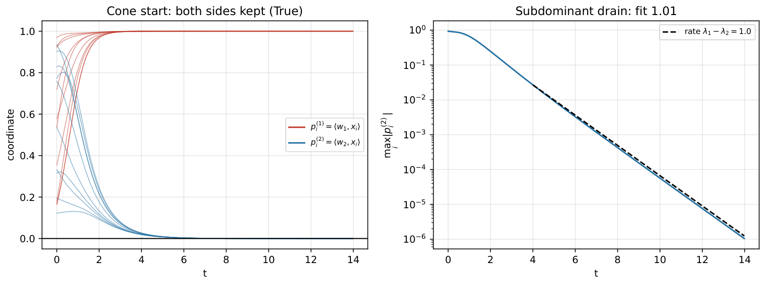
Proposition 3

(Subdominant drain). Let ${\lambda }_k$ ($k\ge 2$) be real with ${\lambda }_k<{\lambda }_1$, and $p_i^{\left(k\right)}=\langle w_k,x_i\rangle =O(\parallel \xi \parallel )$ near $x_i=v_1$ (since $\langle w_k,v_1\rangle =0$). The linearisation of (9) at the collapsed configuration is

$${\dot{p}}^{\left(k\right)}=\left(\frac{{\lambda }_k}{n}\mathbf{1}{\mathbf{1}}^{\top }-{\lambda }_{1}I\right)p^{\left(k\right)}+{O(\parallel \xi \parallel }^2).$$

(10)

Here, $\mathbf{1}={(1,\dots ,1)}^{\top }\in {\mathbb{R}}^n$, so that $\mathbf{1}{\mathbf{1}}^{\top }$ is the $n\times n$ all-ones matrix and $\frac{1}{n}\mathbf{1}{\mathbf{1}}^{\top }$ is the averaging (barycentre) projector onto the consensus direction $\mathbf{1}$. The operator in (10) has eigenvalues ${\lambda }_k$–${\lambda }_1$ on $\mathbf{1}$ (the consensus direction) and $-{\lambda }_1$ on ${\mathbf{1}}^{\perp }$. For ${\lambda }_1>0$, both are negative, so $p^{\left(k\right)}\to 0$: the consensus part drains at the spectral gap rate ${\lambda }_1$–${\lambda }_k$ and the fluctuation part at ${\lambda }_1$—matching the isotropic rate of Theorem 3, since $p_i^{\left(k\right)}=\langle w_k,{\zeta }_i\rangle$ here and ${\dot{\zeta }}_i=-{\lambda }_1{\zeta }_i$ already gives the second rate directly. Hence, the collective set $\{x_i\in w_k^{\perp }\}$ is attracting (the multi-token shadow of the stable manifold of the saddle $v_k$), not a basin separator: which attractor is reached is fixed by $\mathrm{sign}\langle w_1,x\rangle$, transverse to the $w_k$-constraint, so a subdominant positive eigenvalue confines a dynamically irrelevant coordinate, not a competing cluster. Only $k=1$ gives a marginal coordinate, whose consensus direction has an eigenvalue of 0 and is therefore basin-defining.

Proof. 

At collapse $W=\frac{1}{n}\mathbf{1}{\mathbf{1}}^{\top }$ and ${\rho }_i={\lambda }_1+O(\parallel \xi \parallel )$, the $O(\parallel \xi \parallel )$ correction is i-independent to this order, by the same computation as in the proof of Theorem 3: $S_i={\lambda }_1{v}_1+V\overline{\xi }+{O(\parallel \xi \parallel }^2)$ gives ${\rho }_i=\langle v_1+{\xi }_i,S_i\rangle ={\lambda }_1+\langle v_1,V\overline{\xi }\rangle +{O(\parallel \xi \parallel }^2)$, using $\langle {\xi }_i,v_1\rangle =0$). Hence, ${\lambda }_{k}W-D_{\rho }=\frac{{\lambda }_k}{n}\mathbf{1}{\mathbf{1}}^{\top }-{\lambda }_{1}I+O(\parallel \xi \parallel )$, giving (10); since $p^{\left(k\right)}=O(\parallel \xi \parallel )$, the neglected terms are $O(\parallel \xi {\parallel }^2)$. The rank-one matrix $\frac{1}{n}\mathbf{1}{\mathbf{1}}^{\top }$ has an eigenvalue of 1 on $\mathbf{1}$ and 0 on ${\mathbf{1}}^{\perp }$, so the eigenvalues of (10) are ${\lambda }_k$–${\lambda }_1$ (on $\mathbf{1}$) and $-{\lambda }_1$ (on ${\mathbf{1}}^{\perp }$); both are negative when ${\lambda }_1>0>{\lambda }_k-{\lambda }_1$. Setting $k=1$ replaces the first eigenvalue by ${\lambda }_1-{\lambda }_1=0$. For $k=1$, however, $p^{\left(1\right)}$ is $O\left(1\right)$ rather than $O(\parallel \xi \parallel )$, so the linearisation above is not applied to it: the vanishing rate ${\lambda }_1-{\lambda }_1=0$ only records that this direction has no exponential decay (it is marginal), while the sign of the dominant coordinate is preserved exactly and independently by the orthant invariance of Proposition 2. The asymptotic stability of $\pm v_1$ is provided by the fluctuation and mean modes of Theorem 3, not by this zero. For a complex subdominant pair, the two real functionals $\mathrm{Re}{w}_k$ and $\mathrm{Im}{w}_k$ give a coupled pair of coordinates with the same gap-rate decay of ${\lambda }_1$–$\mathrm{Re}{\lambda }_k$, together with rotation at $|\mathrm{Im}{\lambda }_k|$. □

Remark 9

(Two boundary cases). ${\lambda }_k<0$ makes ${\lambda }_k{w}_{ij}<0$, breaking the positivity of the off-diagonal entries, so no trapping (the spreading regime); a complex pair with a positive real part does not trap either, since the real reduction of $\langle w_k,x_i\rangle$ carries a rotation (frequency $|\mathrm{Im}{\lambda }_k|$) that destroys orthant invariance. By contrast, in the one-cluster flow $\frac{d}{dt}\langle w_k,x\rangle =({\lambda }_k-\langle x,Vx\rangle ),\langle w_k,x\rangle$ is sign-preserving for every real eigenvalue regardless of sign—the pure invariant-subspace structure of the invariant-subspace lattice (Supplementary Material), with no off-diagonal positivity hypothesis, because there is no inter-token coupling.

4.3. The Role of Attention: Numerical Results

The preceding results show that, analytically, the attention matrix A cannot override V: the field is ${\dot{x}}_i=P_{x_i}^{\perp }\left(V{m}_i\right)$, with $m_i={\sum }_j{w}_{ij}{x}_j$, a convex mean, so A only reweights the value force (Remark 10). We now report what this means quantitatively, established numerically.

Remark 10

(Clustering dichotomy: when a cluster forms). Three mutually exclusive cases, governed entirely by the dominant spectrum of V:

• ${\mathbf{\lambda }}_{\mathbf{1}}>\mathbf{0}$ real and dominant. The collapsed configuration is fluctuation-stable ($L_{\mathrm{fluct}}=-{\lambda }_{1}I\prec 0$) and tokens cluster, settling on $+v_1$ or $-v_1$ by $\mathrm{sign}\langle w_1,x\rangle$ (Theorem 3).
• ${\mathbf{\lambda }}_{\mathbf{1}}<\mathbf{0}$. Then, $L_{\mathrm{fluct}}=\left|{\lambda }_1\right|I\succ 0$: every transverse direction grows, so no cluster forms—tokens spread regardless of initial data, even within a single hemisphere $\{\langle w_1,x\rangle >0\}$, since that constraint is transverse to the fluctuation mode that decides coherence.
• Complex dominant pair. No point cluster exists: the configuration is carried onto the great-circle limit cycle of the dominant eigenplane (Proposition 1, Remark 6).

This is the pure value-matrix statement; with a u-aligned MLP, the fluctuation operator becomes $P_{v_1}^{\perp }D\mathsf{\Phi }\left(v_1\right)P_{v_1}^{\perp }-{\lambda }_{1}I$, so a sufficiently expansive Φ can hold a cluster together even when ${\lambda }_1<0$—the $L_{\mathrm{col}}$ versus $L_{\mathrm{fluct}}$ tension of Proposition 4.

• Collapse is robust to $\mathit{A}$.

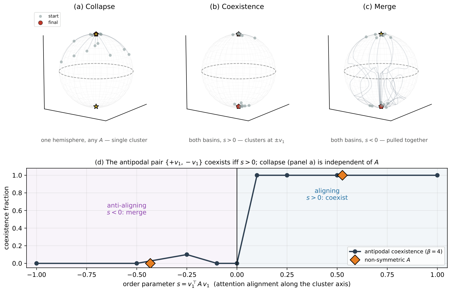
Writing $S_i=V{m}_i$ as above, attention enters only through the convex weights $m_i$: for symmetric V with ${\lambda }_1>0$ and generic one-hemisphere initial data, tokens collapse to the single cluster $v_1$ for every attention matrix tested: $A=I$, symmetric positive-definite, symmetric indefinite, strongly non-symmetric, and negative-definite, as well as across temperatures β (Figure 6a). The only stable clusters are $\pm v_1$. A tight cluster placed at a subdominant eigenvector $v_k$ ($k\ge 2$, ${\lambda }_k>0$) stays internally coherent—its fluctuations decay at rate ${\lambda }_k$—but its centre sits at a saddle of the one-cluster flow (the unstable direction ${\lambda }_1$–${\lambda }_k>0$, Proposition 1), so the cluster migrates to $\pm v_1$ rather than persisting at $v_k$. The genuine multi-cluster state is therefore the antipodal pair $\{+v_1,-v_1\}$ (Figure 6b,c).

• Coexistence versus merger: the order parameter $\mathit{s}={\mathit{v}}_{\mathbf{1}}^{\top }{\mathit{Av}}_{\mathbf{1}}$

Whether two groups occupying the opposite basins coexist or merge is governed by a single scalar,

$$s:=v_1^{\top }A{v}_1,$$

with the alignment of attention along the cluster axis. The leading cross-cluster logit between a $+v_1$ token and a $-v_1$ token is $\beta v_1^{\top }A(-v_1)=-\beta s$, so the clusters coexist when within-cluster attention dominates ($s>0$) and merge when cross-cluster attention dominates ($s<0$), the transition lying at $s=0$ (Figure 6d). Since the antisymmetric part of A drops out of the quadratic form, $s=v_1^{\top }{A}_{\mathrm{sym}}{v}_1$ and a non-symmetric A obey the same law—the relevant case, as a trained attention matrix $A=W_Q^{\top }{W}_K$ is generically non-symmetric and indefinite; negative-definiteness is merely one route to $s<0$, not a distinct mechanism. At large β, the $s<0$ side becomes metastable: a $+v_1$ token attending to the $-v_1$ cluster feels $P_{+v_1}^{\perp }\left({\lambda }_1(-v_1)\right)=0$, a vanishing radial force, so the merger stalls; the clean transition is the diffuse-attention limit.

5. Diagonal MLP

We now switch on the u-aligned MLP Φ together with a symmetric value matrix V. This is the regime in which the one-cluster flow acquires a Lyapunov function and the uncollapsed dynamics inherit multi-token stability automatically; both rest on $D\mathsf{\Phi }$ being symmetric. The gradient, Hessian, and linearisation identities used throughout are collected for reference in the Supplementary Material.

5.1. Lyapunov Structure and One-Cluster Convergence

• One-cluster ODE

When all tokens coincide, $x_i\left(t\right)=x\left(t\right)$ for all i, the weights are uniform ($w_{ij}=1/n$), and (1) reduces to

$$\dot{x}=P_x^{\perp }(Vx+\mathsf{\Phi }\left(x\right)).$$

(11)

Theorem 4

(Lyapunov function). For symmetric V and u-aligned Φ as above, the ODE (11) is the Riemannian gradient flow on $S^{d-1}$ of

$$L\left(x\right)={\displaystyle \frac{1}{2}}\langle x,Vx\rangle +{\displaystyle \sum _{k=1}^r}{\gamma }_k{\int }_0^{\langle u_k,x\rangle }\sigma ({\alpha }_{k}t+b_k)dt.$$

(12)

Along every trajectory, $\dot{L}={\parallel \dot{x}\parallel }^2\ge 0$, with equality if x is a fixed point. By LaSalle’s invariance principle, every trajectory converges to a fixed point. Periodic orbits and chaotic dynamics are impossible.

Proof. 

The construction proceeds in six steps.

• Step 1 ($D\mathsf{\Phi }$ is symmetric). The u-aligned MLP is $\mathsf{\Phi }\left(x\right)={\sum }_{k=1}^r{\gamma }_k\sigma ({\alpha }_k\langle u_k,x\rangle +b_k)u_k$. Its Jacobian is:

$$\begin{array}{c} D\mathsf{\Phi }{\left(x\right)}_{ij}={\displaystyle \frac{\partial {\mathsf{\Phi }}_i}{\partial x_j}}\left(x\right)={\displaystyle \sum _{k=1}^r}{\gamma }_k{\sigma }^{\prime }({\alpha }_k{s}_k+b_k)·{\alpha }_k·{\left(u_k\right)}_j·{\left(u_k\right)}_i\\ ={\displaystyle \sum _{k=1}^r}{\gamma }_k{\alpha }_k{\sigma }^{\prime }({\alpha }_k{s}_k+b_k)·{\left(u_k\right)}_i{\left(u_k\right)}_j,\end{array}$$

(13)

where $s_k=\langle u_k,x\rangle ={\sum }_j{\left(u_k\right)}_j{x}_j$. In matrix form:

$$D\mathsf{\Phi }\left(x\right)={\displaystyle \sum _{k=1}^r}{\gamma }_k{\alpha }_k{\sigma }^{\prime }({\alpha }_k{s}_k+b_k)u_k{u}_k^{\top }.$$

(14)

Since each term $u_k{u}_k^{\top }$ is symmetric and the coefficients ${\gamma }_k{\alpha }_k{\sigma }^{\prime }({\alpha }_k{s}_k+b_k)\in \mathbb{R}$ are scalars, $D\mathsf{\Phi }\left(x\right)$ is symmetric for all x.

• Step 2 ($\mathsf{\Phi }=\nabla g$). Define

$$g\left(x\right)={\displaystyle \sum _{k=1}^r}{\gamma }_k{\int }_0^{\langle u_k,x\rangle }\sigma ({\alpha }_{k}t+b_k)dt.$$

(15)

We verify $\nabla g\left(x\right)=\mathsf{\Phi }\left(x\right)$ by differentiating with respect to $x_j$:

$$\begin{array}{c}{\displaystyle \frac{\partial g}{\partial x_j}}\left(x\right)={\displaystyle \sum _{k=1}^r}{\gamma }_k·{\displaystyle \frac{\partial }{\partial x_j}}{\int }_0^{\langle u_k,x\rangle }\sigma ({\alpha }_{k}t+b_k)dt\\ ={\displaystyle \sum _{k=1}^r}{\gamma }_k·\sigma ({\alpha }_k\langle u_k,x\rangle +b_k)·{\left(u_k\right)}_j={\mathsf{\Phi }}_j\left(x\right),\end{array}$$

(16)

using ${\partial }_j\langle u_k,x\rangle ={\left(u_k\right)}_j$). Hence, $\mathsf{\Phi }=\nabla g$.

• Step 3 ($Vx+\mathsf{\Phi }\left(x\right)=\nabla L\left(x\right)$).

With $f_V\left(x\right)={\displaystyle \frac{1}{2}}\langle x,Vx\rangle$ and $V=V^{\top }$:

$$\nabla f_V\left(x\right)=Vx.$$

(17)

Indeed,

$${\partial }_{x_j}\left({\displaystyle \frac{1}{2}}\sum _{i,k}{V}_{ik}{x}_i{x}_k\right)={\displaystyle \frac{1}{2}}\sum _k{V}_{jk}{x}_k+{\displaystyle \frac{1}{2}}\sum _i{V}_{ij}{x}_i=\sum _k{V}_{jk}{x}_k={\left(Vx\right)}_j$$

using $V=V^{\top }$.

Therefore,

$$\nabla L=\nabla f_V+\nabla g=Vx+\mathsf{\Phi }\left(x\right).$$

(18)

• Step 4 (The ODE is a Riemannian gradient flow). We use the following criterion. A vector field of the form $F\left(x\right)=P_x^{\perp }h\left(x\right)$ on $S^{d-1}$ (with $h:{\mathbb{R}}^d\to {\mathbb{R}}^d$) is a Riemannian gradient flow of some potential if its covariant Jacobian $P_x^{\perp }Dh\left(x\right)P_x^{\perp }$ is self-adjoint on $T_x{S}^{d-1}$ for every x; this is the integrability (symmetric-Hessian) condition for a gradient on a Riemannian manifold, and for $h=\nabla L$ it is automatic, but we verify it directly from the model. Here, $h\left(x\right)=Vx+\mathsf{\Phi }\left(x\right)$, so $Dh\left(x\right)=V+D\mathsf{\Phi }\left(x\right)$ and the covariant Jacobian is $P_x^{\perp }(V+D\mathsf{\Phi }\left(x\right))P_x^{\perp }$. Since $V=V^{\top }$ and $D\mathsf{\Phi }\left(x\right)=D\mathsf{\Phi }{\left(x\right)}^{\top }$ (Step 1), the sum $V+D\mathsf{\Phi }\left(x\right)$ is symmetric, so the compression $P_x^{\perp }(V+D\mathsf{\Phi }\left(x\right))P_x^{\perp }$ is self-adjoint on $T_x{S}^{d-1}$. The criterion is therefore met at every x, confirming $\dot{x}=P_x^{\perp }(Vx+\mathsf{\Phi }\left(x\right))={\mathrm{grad}}_{S}L\left(x\right)$.
• Step 5 ($\dot{L}={\parallel \dot{x}\parallel }^2$). Along a trajectory of the ODE, set $w=\nabla L\left(x\right)=Vx+\mathsf{\Phi }\left(x\right)$ and split it into its tangential and normal parts at x,

$$w=P_x^{\perp }w+\langle x,w\rangle x,P_x^{\perp }w={\mathrm{grad}}_{S}L\left(x\right)\in T_x{S}^{d-1},$$

(19)

with the tangential part being, by definition, the Riemannian gradient. Using $\dot{x}=P_x^{\perp }w$ together with (19) and bilinearity,

$$\begin{array}{cc}\hfill {\displaystyle \frac{d}{dt}}L\left(x\left(t\right)\right)& =\langle \nabla L\left(x\right),\dot{x}\rangle =\langle w,P_x^{\perp }w\rangle \hfill \\ \hfill & =\langle P_x^{\perp }w+\langle x,w\rangle x,P_x^{\perp }w\rangle \hfill \\ \hfill & =\langle {\mathrm{grad}}_{S}L,P_x^{\perp }w\rangle +\langle x,w\rangle \langle x,P_x^{\perp }w\rangle .\hfill \end{array}$$

The second term vanishes because $P_x^{\perp }w={\mathrm{grad}}_{S}L\in T_x{S}^{d-1}$ is orthogonal to x, i.e., $\langle x,P_x^{\perp }w\rangle =0$ (equivalently, the ODE preserves $\parallel x\parallel = 1$, so $\langle x,\dot{x}\rangle =0$). Therefore:

$$\dot{L} = \langle {\mathrm{grad}}_{S}L\left(x\right),\dot{x}\rangle =\langle {\mathrm{grad}}_{S}L\left(x\right),{\mathrm{grad}}_{S}L\left(x\right)\rangle =\parallel {\mathrm{grad}}_S{L\left(x\right)\parallel }^2={\parallel \dot{x}\parallel }^2\ge 0.$$

(20)

• Step 6 (Convergence). L is continuous on the compact manifold $S^{d-1}$, hence bounded. $\dot{L}={\parallel \dot{x}\parallel }^2\ge 0$, so L is non-decreasing along trajectories. By LaSalle’s invariance principle, every trajectory converges to the largest invariant set contained in $\{\dot{L}=0\}=\{\parallel \dot{x}\parallel = 0\}=\{x:{\mathrm{grad}}_{S}L\left(x\right)=0\}$, which is the set of critical points of L on $S^{d-1}$.

Since $S^{d-1}$ is compact and L is bounded and non-decreasing, the ω-limit set of every trajectory is non-empty and invariant, hence contained in the critical point set. Convergence to a single critical point follows when the critical points are isolated, which holds for generic $(V,\mathsf{\Phi })$. When they are not isolated (for instance, when V has a repeated eigenvalue, so that the critical set contains submanifolds rather than isolated points), L is a Morse–Bott function along the gradient flow, and every trajectory still converges to a single connected component of the critical set (the ω-limit set of a gradient flow of an analytic, or Morse–Bott, potential is a single critical component). The convergence conclusion is therefore unchanged; only the limit may be a critical manifold rather than a point.

Periodic orbits are excluded because L is strictly increasing along any non-constant trajectory. □

Corollary 1

(Fixed points and stability). The fixed points of (11) are the critical points of L on $S^{d-1}$: solutions of $Vx+\mathsf{\Phi }\left(x\right)=\mu x$. When the $u_k$ are eigenvectors of V with eigenvalues ${\nu }_k$, this decouples as

$${\nu }_k{s}_k+{\gamma }_k\sigma ({\alpha }_k{s}_k+b_k)=\mu s_k,k=1,\dots ,r,s_1^2+...+s_r^2=1.$$

(21)

A critical point $x^{\ast }$ is a stable attractor if it has a strict local maximum of L (Riemannian Hessian negative definite; derived in the Supplementary Material); it is an unstable saddle if the Hessian has at least one positive eigenvalue. The global attractor (from generic initial conditions) is the global maximum of L.

Remark 11

(Role of V in attractor selection). The global maximum of $L=f_V+g$ balances the Rayleigh quotient of V (favouring eigenvectors of V with large eigenvalues) against the MLP potential g (favouring directions where g is large). Increasing ${\nu }_k$ shifts the global maximum toward $u_k$: a large ${\nu }_k$ makes $S^{d-1}$ tilt in the $u_k$ direction. The value matrix thus participates directly in attractor selection, in contrast to the attention matrix A, which drives the collapse to a single cluster but does not select among critical points.

5.2. Uncollapsed Token Dynamics

Proposition 4 below shows that for general V and Φ, a stable one-cluster fixed point need not be stable for the multi-token system. We now show that the u-aligned MLP with symmetric V is a special case where this instability is excluded: the gradient flow structure automatically guarantees multi-token stability at every attractor.

We consider n tokens near a critical point $x^{\ast }$ of L: $x_i=x^{\ast }+{\xi }_i$, decomposed as ${\xi }_i=\overline{\xi }+{\zeta }_i$ (mean plus fluctuation, ${\sum }_i{\zeta }_i=0$).

• Mean mode

At first order in $\parallel \xi \parallel$: ${\sum }_j{w}_{ij}V{x}_j\approx V(x^{\ast }+\overline{\xi })$ and $\mathsf{\Phi }\left(x_i\right)\approx \mathsf{\Phi }\left(x^{\ast }\right)+D\mathsf{\Phi }\left(x^{\ast }\right)(\overline{\xi }+{\zeta }_i)$. Averaging over i and using ${\sum }_i{\zeta }_i=0$:

$$\dot{\overline{\xi }}=P_{x^{\ast }}^{\perp }\left({\nabla }^{2}L\left(x^{\ast }\right)\overline{\xi }\right)+{O(\parallel \xi \parallel }^2) = \left({\mathrm{Hess}}_{S}L{|}_{x^{\ast }}\right)\overline{\xi }+{O(\parallel \xi \parallel }^2).$$

(22)

At a local maximum of L, ${\mathrm{Hess}}_S{L|}_{x^{\ast }}$ is negative definite, so $\overline{\xi }\to 0$: the cluster mean converges to $x^{\ast }$. At a saddle, the mean grows in the unstable Hessian direction, driving the cluster toward the global maximum of L.

• Fluctuation modes

Since Φ acts independently on each token and ${\sum }_i{\zeta }_i=0$, the MLP contributes $P_{x^{\ast }}^{\perp }\left(D\mathsf{\Phi }\left(x^{\ast }\right){\zeta }_i\right)$ to ${\dot{\zeta }}_i$ and the curvature correction contributes $-\mu {\zeta }_i$ (the same normal-force term as in $L_{\mathrm{col}}$); the softmax attention contributes nothing at first order (Supplementary Material). Combined,

$${\dot{\zeta }}_i=\underset{\mathrm{MLP}}{\underbrace{P_{x^{\ast }}^{\perp }D\mathsf{\Phi }\left(x^{\ast }\right){\zeta }_i}} - \underset{\mathrm{Curvature}}{\underbrace{\mu {\zeta }_i}}+{O(\parallel \xi \parallel }^2)=L_{\mathrm{fluct}}{\zeta }_i+{O(\parallel \xi \parallel }^2).$$

(23)

Writing ${\mathrm{Hess}}_S{g|}_{x^{\ast }}=P_{x^{\ast }}^{\perp }D\mathsf{\Phi }\left(x^{\ast }\right)P_{x^{\ast }}^{\perp }-{\mu }_{\mathsf{\Phi }}I$ for the Riemannian Hessian of the MLP potential and using $\mu ={\mu }_V+{\mu }_{\mathsf{\Phi }}$, the operator is $L_{\mathrm{fluct}}={\mathrm{Hess}}_S{g|}_{x^{\ast }}-{\mu }_{V}I$. At a local maximum of L, one has ${\mathrm{Hess}}_S{g|}_{x^{\ast }}⪯({\mu }_V-\eta )I$ (because ${\mathrm{Hess}}_{S}L⪯-\eta I$ and $P_{x^{\ast }}^{\perp }V{P}_{x^{\ast }}^{\perp }⪰0$ for $V⪰0$), hence $L_{\mathrm{fluct}}⪯-\eta I\prec 0$: all fluctuation eigenvalues are negative near a local maximum of L.

Theorem 5

(Uncollapsed token dynamics). Let $x^{\ast }$ be a critical point of L on $S^{d-1}$.

(i) 

(Collapse.) If $x^{\ast }$ is a local maximum of L, both mean and fluctuation modes decay. Every trajectory of (1) near $(x^{\ast },\dots ,x^{\ast })$ converges to $(x^{\ast },\dots ,x^{\ast })$: tokens collapse to the stable attractor.

(ii) 

(Saddle escape.) Suppose $x^{\ast }$ is a saddle of L and the fluctuation-stability condition

$$L_{\mathrm{fluct}}=P_{x^{\ast }}^{\perp }D\mathsf{\Phi }\left(x^{\ast }\right)P_{x^{\ast }}^{\perp }-\mu I\prec 0\mathit{on}{T}_{x^{\ast }}{S}^{d-1}$$

(24)

holds (equivalently, ${\mathrm{Hess}}_S{g|}_{x^{\ast }}\prec {\mu }_{V}I$; a sufficient explicit form is ${\max }_{1\le k\le r}{\left({\gamma }_k{\alpha }_k{\sigma }^{\prime }({\alpha }_k{s}_k^{\ast }+b_k)\right)}^{+}<\mu$, which, in particular, forces $\mu >0$). Then, the mean mode grows in the unstable Hessian direction, driving the cluster toward the global maximum of L, while every fluctuation mode decays: the tokens stay clustered while the cluster escapes the saddle. Condition (24) holds automatically at a local maximum (part (i)); at a saddle, it is a genuine restriction, and if it fails, the saddle drives the tokens apart instead of keeping them clustered.

Proof. 

Part (i): At a local maximum, ${\mathrm{Hess}}_{S}L$ is negative definite, so both (22) and the fluctuation operator in (23) have all negative eigenvalues. Part (ii): The mean operator is $L_{\mathrm{col}}={\mathrm{Hess}}_S{L|}_{x^{\ast }}$ and the fluctuation operator is $L_{\mathrm{fluct}}={\mathrm{Hess}}_S{g|}_{x^{\ast }}-{\mu }_{V}I$. At a saddle, $L_{\mathrm{col}}$ has an eigenvalue ${\lambda }_{+}>0$ with eigenvector $v_{+}\in T_{x^{\ast }}{S}^{d-1}$, so, by (22), the mean grows, $\overline{\xi }\left(t\right)\sim e^{{\lambda }_{+}t}{v}_{+}$, and the cluster leaves the neighbourhood of $x^{\ast }$ along $v_{+}$ toward the global maximum of L. Condition (24) makes $L_{\mathrm{fluct}}$ negative definite, so, by (23), every fluctuation mode decays ${\zeta }_i\left(t\right)\to 0$ at an exponential rate bounded away from zero. Hence, the inter-token spread ${\max }_i\parallel {\zeta }_i\parallel$ contracts while the common mean escapes: the tokens remain clustered throughout. If, instead, (24) fails, then $\langle v,L_{\mathrm{fluct}}v\rangle >0$ for some $v\in T_{x^{\ast }}{S}^{d-1}$ and that fluctuation direction grows—the saddle drives the tokens apart, which is the multi-token instability of Proposition 4(ii). □

Remark  12

(Why the u-aligned case resolves the generic instability). Proposition 4(ii) below identifies a potential conflict: V may stabilise the one-cluster ODE without stabilising the fluctuations. The u-aligned MLP with symmetric V avoids this by construction. Since V and $D\mathsf{\Phi }\left(x^{\ast }\right)$ share eigenvectors $u_k$, the operators differ only by $L_{\mathrm{fluct}}-L_{\mathrm{col}}=-P_{x^{\ast }}^{\perp }V{P}_{x^{\ast }}^{\perp }$, so for symmetric positive semi-definite V the eigenvalue correction is $-q_V\left(v\right)\le 0$, so ${\lambda }_{\mathrm{fluct}}\left(v\right)\le {\lambda }_{\mathrm{col}}\left(v\right)<0$. The gradient flow structure ensures that ${\lambda }_{\mathrm{col}}\left(v\right)<0$ everywhere, and since the correction is negative, ${\lambda }_{\mathrm{fluct}}\left(v\right)<{\lambda }_{\mathrm{col}}\left(v\right)<0$: fluctuation modes are more stable than collapsed modes.

• Numerical verification of the $\mathit{u}$-aligned MLP results

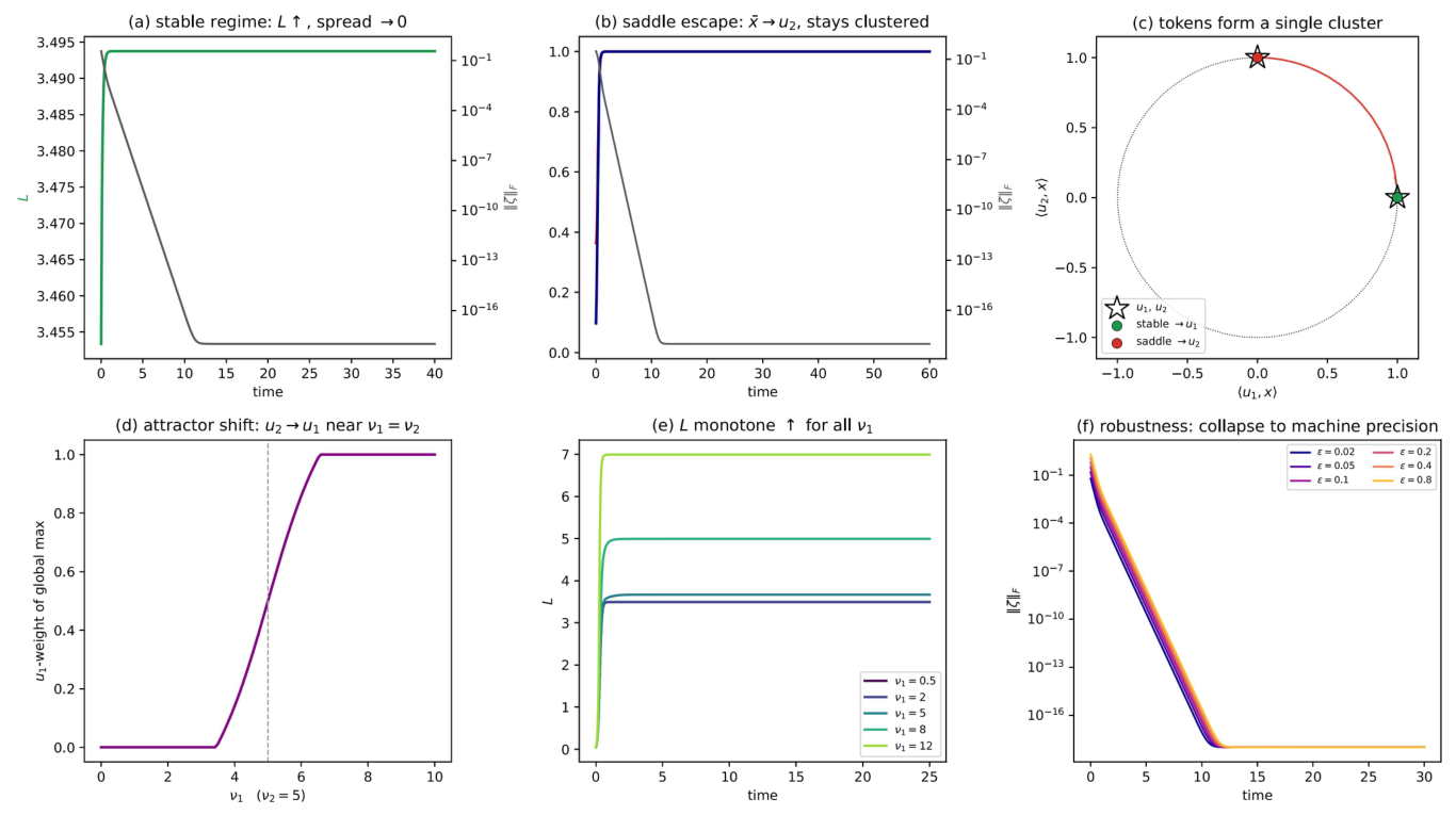
We use $d=64$, $r=2$, $n=10$, $\beta =2$, $A=2u_1{u}_1^{\top }$, ${\gamma }_k=1.5$, ${\alpha }_k=2$, $b_k=0$, tanh activation, and step size $dt=0.05$. Figure 7 shows six experiments with two parameter regimes: (i) stable regime with ${\nu }_c=(5,0.1)$, global max of L near $u_1$; (ii) saddle regime using ${\nu }_s=(0.5,5)$, for which $x_c^{\ast }\approx u_1$ is a saddle of $L_s$ and $u_2$ is the global maximum.

• Panels (a) and (b): stable attractor

Starting near the global max $x_c^{\ast }\approx u_1$ under $L_c$: L increases monotonically and ${\parallel \zeta \parallel }_F\to 0$ (panel (a)). Starting near the same point under $L_s$ (where it is a saddle): $L_s$ still increases monotonically and ${\parallel \zeta \parallel }_F\to 0$, but $|\langle u_2,\overline{x}\rangle |\to 1$ (panel (b)). The cluster escapes the saddle while staying clustered, confirming Theorem 5(ii).

• Panel (c): Token positions

Projected onto $(u_1,u_2)$: stable-regime tokens (green) all converge to $u_1$; saddle-escape tokens (red) converge to $u_2$. In both cases, tokens form a single cluster at the final position.

• Panel (d): Attractor shift

Varying ${\nu }_1$ with ${\nu }_2=5$ fixed: the global maximum transitions from $u_2$-dominated (small ${\nu }_1$) to $u_1$-dominated (large ${\nu }_1$), with a smooth crossover near ${\nu }_1\approx {\nu }_2=5$. This confirms Remark 11.

• Panel (e): L monotone for all ${\nu }_1$

From a common random initialisation, L increases monotonically to different attractor values for five values of ${\nu }_1$, confirming Theorem 4 uniformly.

• Panel (f): Robustness

Six perturbation sizes near the stable $x^{\ast }$ all collapse at machine precision, confirming Theorem 5(i).

6. One-Cluster vs. Multi-Token: The General Mechanism

We establish a general relationship between one-cluster stability and multi-token stability for arbitrary V and Φ.

• Linearisation at a fixed point

Let $x^{\ast }$ be a fixed point: $P_{x^{\ast }}^{\perp }(V{x}^{\ast }+\mathsf{\Phi }\left(x^{\ast }\right))=0$, i.e., $V{x}^{\ast }+\mathsf{\Phi }\left(x^{\ast }\right)=\mu x^{\ast }$ with $\mu =\langle x^{\ast },V{x}^{\ast }+\mathsf{\Phi }\left(x^{\ast }\right)\rangle$. Write ${\mu }_V=\langle x^{\ast },V{x}^{\ast }\rangle$ for the normal component of the value matrix. For standard softmax attention, the linearised attention force is independent of the attention matrix and common to all tokens at first order, so it acts only on the mean and contributes no first-order term to the fluctuations (this is established self-containedly in Proposition 5 below). The clustering of fluctuations is therefore carried entirely by the curvature term ${\mu }_V$, and the relevant linearisation operators on $T_{x^{\ast }}{S}^{d-1}$ are as follows (derived below in (39)):

$$\begin{array}{cc}\hfill L_{\mathrm{col}}& =P_{x^{\ast }}^{\perp }(V+D\mathsf{\Phi }\left(x^{\ast }\right))P_{x^{\ast }}^{\perp }-\mu I,\hfill \end{array}$$

(25)

$$\begin{array}{cc}\hfill L_{\mathrm{fluct}}& =P_{x^{\ast }}^{\perp }D\mathsf{\Phi }\left(x^{\ast }\right)P_{x^{\ast }}^{\perp }-\mu I,\hfill \end{array}$$

(26)

where both operators carry the same curvature term $-\mu I$, $\mu ={\mu }_V+{\mu }_{\mathsf{\Phi }}$, arising from the normal force $\mu x^{\ast }$ at the collapsed fixed point. Note that the tangential action of V (the form $q_V$) is absent from $L_{\mathrm{fluct}}$: the value matrix term ${\sum }_j{w}_{ij}V{x}_j\approx V\overline{x}$ contributes only to the mean mode, not to fluctuations at first order. (V’s normal component ${\mu }_V$ is present in both operators through μ and cancels when they are compared.)

• Relationship

Throughout this comparison, we write ${\lambda }_{\mathrm{col}}\left(v\right)=\langle v,L_{\mathrm{col}}v\rangle$, ${\lambda }_{\mathrm{fluct}}\left(v\right)=\langle v,L_{\mathrm{fluct}}v\rangle$, and $q_V\left(v\right)=\langle v,P_{x^{\ast }}^{\perp }Vv\rangle$ for the quadratic forms (Rayleigh quotients) of the linearisation operators on the tangent space. Since $L_{\mathrm{col}}-L_{\mathrm{fluct}}=P_{x^{\ast }}^{\perp }V{P}_{x^{\ast }}^{\perp }$, these satisfy

$${\lambda }_{\mathrm{fluct}}\left(v\right)={\lambda }_{\mathrm{col}}\left(v\right)-q_V\left(v\right)$$

(27)

as an identity of quadratic forms, valid for arbitrary (possibly non-symmetric) V.

For a symmetric operator, the Rayleigh quotient attains the eigenvalues at its stationary values, so ${\max }_v{\lambda }_{\mathrm{col}}\left(v\right)$ is the top eigenvalue and the sign of the form decides stability. For a non-symmetric $L_{\mathrm{col}}$ (non-symmetric V), this fails: ${\max }_v{\lambda }_{\mathrm{col}}\left(v\right)$ is the numerical abscissa (the top eigenvalue of the symmetric part $\frac{1}{2}(L_{\mathrm{col}}+L_{\mathrm{col}}^{\top })$), an upper bound for the spectral abscissa ${\max }_j\mathrm{Re}\mathrm{spec}\left(L_{\mathrm{col}}\right)$ that can be strictly larger. Consequently, the collapse criterion of Proposition 4(i) is a sufficient condition: it forces the numerical abscissa of $L_{\mathrm{fluct}}$ below zero, hence giving monotone (not merely asymptotic) decay. The exact one-cluster spectrum for non-symmetric V is obtained spectrally by the deflation Lemma 2 ($\mathrm{spec}\left(A_k\right)=\{{\lambda }_j-{\lambda }_k\}$), not from these quadratic forms; we use the form-level relation (27) only for the sufficient comparison below.

Proposition 4

(One-cluster vs. multi-token stability). Let $\eta =-{\max }_v{\lambda }_{\mathrm{col}}\left(v\right)>0$ be the one-cluster stability margin (in the numerical-range sense above).

(i) 

(Sufficient condition for collapse.) If V is positive semi-definite on $T_{x^{\ast }}{S}^{d-1}$ ($q_V\left(v\right)\ge 0$ for all $v\perp x^{\ast }$), then ${\lambda }_{\mathrm{fluct}}\left(v\right)\le -\eta <0$ for every unit $v\perp x^{\ast }$: all fluctuation eigenvalues are negative and the tokens collapse to $x^{\ast }$. No further condition is required.

(ii) 

(Possible instability.) For general V and Φ, there exist configurations where ${\lambda }_{\mathrm{col}}\left(v\right)<0$ (one-cluster stable) but ${\lambda }_{\mathrm{fluct}}\left(v\right)>0$ (tokens spread). This occurs when V is contractive in direction v (stabilising the mean but not the fluctuations), while $D\mathsf{\Phi }\left(x^{\ast }\right)$ is expansive in v.

Proof. 

The eigenvalue relation. For any $v\in T_{x^{\ast }}{S}^{d-1}$ with $\parallel v\parallel = 1$, write $q_V\left(v\right)=\langle v,P_{x^{\ast }}^{\perp }Vv\rangle$ and $q_{D\mathsf{\Phi }}\left(v\right)=\langle v,P_{x^{\ast }}^{\perp }D\mathsf{\Phi }\left(x^{\ast }\right)v\rangle$. From operators (25) and (26):

$$\begin{array}{cc}\hfill {\lambda }_{\mathrm{col}}\left(v\right)& =q_V\left(v\right)+q_{D\mathsf{\Phi }}\left(v\right)-\mu ,\hfill \end{array}$$

(28)

$$\begin{array}{cc}\hfill {\lambda }_{\mathrm{fluct}}\left(v\right)& =q_{D\mathsf{\Phi }}\left(v\right)-\mu .\hfill \end{array}$$

(29)

Subtracting:

$${\lambda }_{\mathrm{fluct}}\left(v\right)-{\lambda }_{\mathrm{col}}\left(v\right)=-q_V\left(v\right).$$

(30)

This is the key relation. It shows that the tangential action of V, encoded in the quadratic form $q_V\left(v\right)$, enters ${\lambda }_{\mathrm{col}}$ but not ${\lambda }_{\mathrm{fluct}}$. (The normal component ${\mu }_V$ enters both operators equally through $\mu ={\mu }_V+{\mu }_{\mathsf{\Phi }}$ and therefore cancels in the difference (30).) For positive semi-definite V ($q_V\ge 0$), the fluctuation mode is more stable than the collapsed mode: ${\lambda }_{\mathrm{fluct}}\left(v\right)\le {\lambda }_{\mathrm{col}}\left(v\right)$. For indefinite V, $q_V\left(v\right)<0$ is possible; either effect can make ${\lambda }_{\mathrm{fluct}}\left(v\right)>{\lambda }_{\mathrm{col}}\left(v\right)$, so that fluctuations are less stable than the mean and potentially unstable even when ${\lambda }_{\mathrm{col}}<0$.

Part (i) Sufficient condition. We want to show that ${\lambda }_{\mathrm{fluct}}\left(v\right)<0$ for all $v\perp x^{\ast }$, given that $x^{\ast }$ is one-cluster stable ($\eta =-{\max }_v{\lambda }_{\mathrm{col}}\left(v\right)>0$) and V is positive semi-definite on $T_{x^{\ast }}{S}^{d-1}$.

From (30):

$${\lambda }_{\mathrm{fluct}}\left(v\right)={\lambda }_{\mathrm{col}}\left(v\right)-q_V\left(v\right).$$

(31)

Since $V⪰0$ on $T_{x^{\ast }}{S}^{d-1}$, we have $q_V\left(v\right)\ge 0$. From the one-cluster stability margin, ${\lambda }_{\mathrm{col}}\left(v\right)\le -\eta$ for all units $v\perp x^{\ast }$. Substituting into (31) and using $q_V\left(v\right)\ge 0$ yields:

$${\lambda }_{\mathrm{fluct}}\left(v\right)={\lambda }_{\mathrm{col}}\left(v\right)-q_V\left(v\right)\le -\eta =-\eta <0,$$

(32)

the last inequality by the hypothesis $\eta >0$. This holds for any $V⪰0$ and any $\eta ,C$ with $\eta >0$. The value matrix enters the fluctuation eigenvalue only through the stabilising $q_V\left(v\right)\ge 0$; the only role of the attention is through the bound, involving neither ${\lambda }_{\max }\left(V\right)$ nor ${\mu }_V$.

Part (ii) (An explicit instability). We construct explicit parameters. Let $d=2$, $x^{\ast }=e_1={(1,0)}^{\top }$, $T_{x^{\ast }}{S}^1=\mathrm{span}\left(e_2\right)$. Set $V=-\kappa e_2{e}_2^{\top }$ (contractive on $T_{x^{\ast }}{S}^1$, $q_V\left(e_2\right)=-\kappa <0$, so V is indefinite), $D\mathsf{\Phi }\left(x^{\ast }\right)e_2=\varphi e_2$ with $\varphi >C$ (MLP expansive), and ${\mu }_V=\langle e_1,V{e}_1\rangle =0$.

Then, writing $\mu ={\mu }_V+{\mu }_{\mathsf{\Phi }}={\mu }_{\mathsf{\Phi }}$ (since ${\mu }_V=0$), with ${\mu }_{\mathsf{\Phi }}=\langle x^{\ast },\mathsf{\Phi }\left(x^{\ast }\right)\rangle$ the normal component of the MLP map from the Supplementary Material (not the Jacobian normal component $\langle x^{\ast },D\mathsf{\Phi }\left(x^{\ast }\right)x^{\ast }\rangle$), yields:

$$\begin{array}{cc}\hfill {\lambda }_{\mathrm{col}}\left(e_2\right)& =q_V\left(e_2\right)+q_{D\mathsf{\Phi }}\left(e_2\right)-\mu =-\kappa +\varphi -{\mu }_{\mathsf{\Phi }},\hfill \end{array}$$

(33)

$$\begin{array}{cc}\hfill {\lambda }_{\mathrm{fluct}}\left(e_2\right)& =q_{D\mathsf{\Phi }}\left(e_2\right)-\mu =\varphi -{\mu }_{\mathsf{\Phi }},\hfill \end{array}$$

(34)

at the fixed point $V{e}_1=0$, so $\mathsf{\Phi }\left(e_1\right)=\mu x^{\ast }={\mu }_{\mathsf{\Phi }}{e}_1$; choosing the MLP so that $\mathsf{\Phi }\left(e_1\right)=0$ gives ${\mu }_{\mathsf{\Phi }}=0$. This is consistent with $D\mathsf{\Phi }\left(e_1\right)e_2=\varphi e_2\ne 0$: the map vanishes at $e_1$ while its Jacobian there is expansive in the tangent direction. Then,

$$\begin{array}{cc}\hfill {\lambda }_{\mathrm{col}}\left(e_2\right)& =-\kappa +\varphi ,\hfill \end{array}$$

(35)

$$\begin{array}{cc}\hfill {\lambda }_{\mathrm{fluct}}\left(e_2\right)& =\varphi .\hfill \end{array}$$

(36)

Choose $C<\varphi <\kappa$ (possible since C and ϕ can be chosen freely with $\varphi >C$, then $\kappa >\varphi$):

$${\lambda }_{\mathrm{col}}\left(e_2\right)=\varphi -\kappa <0\left(\mathrm{stable}\right),{\lambda }_{\mathrm{fluct}}\left(e_2\right)=\varphi >0\left(\mathrm{unstable}\right).$$

This confirms that a stable one-cluster fixed point can be multi-token unstable. The mechanism: V is contractive on the tangent space ($-\kappa <0$) providing one-cluster stability, but does not appear in ${\lambda }_{\mathrm{fluct}}$, which is governed by $\varphi >0$. □

Remark 13

(The curvature term is the full $\mu$). Both $L_{\mathrm{col}}$ and $L_{\mathrm{fluct}}$ contain the same curvature term $-\mu I$ with the full $\mu ={\mu }_V+{\mu }_{\mathsf{\Phi }}$, originating from the normal force $\mu x^{\ast }$ at the collapsed fixed point (see (25) and (26) and the linearisation in the Supplementary Material). In particular, the curvature term is not $-{\mu }_{\mathsf{\Phi }}I$ (which would omit the normal component of the value matrix) and not $-{\mu }_{D\mathsf{\Phi }}I$ (the Jacobian normal component, a different object, cf. the Supplementary Material). Because ${\mu }_V$ appears identically in both eigenvalues, it cancels in the difference (30), leaving ${\lambda }_{\mathrm{fluct}}\left(v\right)={\lambda }_{\mathrm{col}}\left(v\right)-q_V\left(v\right)$, with no residual ${\mu }_V$.

Remark 14

(Interpretation). The key asymmetry is that the tangential action of V (the form $q_V$) appears in $L_{\mathrm{col}}$ but not in $L_{\mathrm{fluct}}$. A value matrix that stabilises the one-cluster ODE by being contractive in some tangential direction v provides no corresponding stability to the fluctuation modes in that direction. The fluctuation stability depends entirely on $D\mathsf{\Phi }\left(x^{\ast }\right)$ (and, in the MLP-free case, on the sign of ${\mu }_V$). This asymmetry is the source of the potential discrepancy between one-cluster and multi-token stability for general V and Φ.

• The attention force and the linearised operators (main-text derivation)

We close the section by recording the derivation of (25) and (26) and the proof that softmax attention contributes no first-order clustering force. Place n tokens at $x_i=x^{\ast }+{\xi }_i$ with ${\xi }_i\in T_{x^{\ast }}{S}^{d-1}$, and split ${\xi }_i=\overline{\xi }+{\zeta }_i$, $\overline{\xi }=\frac{1}{n}{\sum }_i{\xi }_i$, ${\sum }_i{\zeta }_i=0$.

Proposition 5

(No first-order attention clustering force). For standard softmax attention with any coupling matrix A, the attention-weighted value force satisfies

$$\sum _j{w}_{ij}V{x}_j=V{x}^{\ast }+V\overline{\xi }+{O(\parallel \xi \parallel }^2)$$

(37)

independent of the token index i to first order. Hence, the attention force drives only the mean mode $\overline{\xi }$ and contributes no first-order term to the fluctuations ${\zeta }_i$.

Proof. 

Linearising the score $\beta \langle x_i,A{x}_j\rangle /\sqrt{d}$ about $x_i=x_j=x^{\ast }$ gives, after softmax normalisation,

$$w_{ij}={\displaystyle \frac{1}{n}}+{\displaystyle \frac{\beta }{n\sqrt{d}}}{\left(A^{\top }{x}^{\ast }\right)}^{\top }({\xi }_j-\overline{\xi })+{O(\parallel \xi \parallel }^2),$$

(38)

in which the query deviation ${\xi }_i$ cancels in the softmax denominator, so the first-order correction depends on the key index j only. Hence,

$$\sum _j{w}_{ij}V{x}_j={\displaystyle \frac{1}{n}}\sum _{j}V(x^{\ast }+{\xi }_j)+\sum _j\left(w_{ij}-\frac{1}{n}\right)V{x}^{\ast }+{O(\parallel \xi \parallel }^2).$$

The first sum is $V{x}^{\ast }+V\overline{\xi }$; in the second, ${\sum }_j(w_{ij}-1/n)=0$ (the rows of W sum to one) multiplies the i-independent vector $V{x}^{\ast }$ to zero, while the correction acting on $V{\xi }_j$ is $O(\parallel \xi {\parallel }^2)$. This gives (37), common to all i; subtracting the mean of the linearised Equation (39) removes this common term, so it contributes nothing to ${\dot{\zeta }}_i$ at first order. □

The linearised operators follow. Expanding ${\dot{x}}_i=P_{x_i}^{\perp }\left({\sum }_j{w}_{ij}V{x}_j+\mathsf{\Phi }\left(x_i\right)\right)$ to first order, using (37), $\mathsf{\Phi }\left(x_i\right)=\mathsf{\Phi }\left(x^{\ast }\right)+D\mathsf{\Phi }\left(x^{\ast }\right){\xi }_i+{O(\parallel \xi \parallel }^2)$, $V{x}^{\ast }+\mathsf{\Phi }\left(x^{\ast }\right)=\mu x^{\ast }$, and $P_{x^{\ast }+{\xi }_i}^{\perp }=P_{x^{\ast }}^{\perp }-{\xi }_i{x}^{\ast \top }-x^{\ast }{\xi }_i^{\top }+{O(\parallel \xi \parallel }^2)$, gives

$${\dot{\xi }}_i=P_{x^{\ast }}^{\perp }\left(V\overline{\xi }+D\mathsf{\Phi }\left(x^{\ast }\right){\xi }_i\right)-\mu {\xi }_i+{O(\parallel \xi \parallel }^2).$$

(39)

The value matrix acts on the mean $\overline{\xi }$ only, whereas the MLP acts on the full deviation ${\xi }_i=\overline{\xi }+{\zeta }_i$. Averaging (39) over i gives $\dot{\overline{\xi }}=(P_{x^{\ast }}^{\perp }(V+D\mathsf{\Phi }\left(x^{\ast }\right))P_{x^{\ast }}^{\perp }-\mu I)\overline{\xi }=L_{\mathrm{col}}\overline{\xi }$, which is (25); subtracting the mean equation, the common term $P_{x^{\ast }}^{\perp }V\overline{\xi }$ cancels and ${\dot{\zeta }}_i=(P_{x^{\ast }}^{\perp }D\mathsf{\Phi }\left(x^{\ast }\right)P_{x^{\ast }}^{\perp }-\mu I){\zeta }_i=L_{\mathrm{fluct}}{\zeta }_i$, which is (26). The value matrix is thus absent from $L_{\mathrm{fluct}}$: it enters only through the common mean.

7. Discussion

The paper establishes two results at different levels of generality.

• Summary

The first (Proposition 4) is a general structural observation: for arbitrary V and Φ, a stable fixed point of the one-cluster ODE need not be stable for the multi-token system. The asymmetry arises because V enters the mean operator $L_{\mathrm{col}}$ but not the fluctuation operator $L_{\mathrm{fluct}}$ (Section 6): the value matrix can stabilise the mean without stabilising the fluctuations, and a spreading instability occurs when V is contractive in some tangential direction while $D\mathsf{\Phi }\left(x^{\ast }\right)$ is expansive there. The second result (Theorems 4 and 5) shows that the u-aligned MLP with symmetric V is the exactly solvable case in which this instability is structurally excluded: the one-cluster flow is the gradient ascent of $L=f_V+g$, every trajectory converges to a critical point, and the tokens collapse to a single cluster at every stable attractor, escaping saddles while remaining clustered.

• The value matrix, not the attention, selects the cluster

A recurring conclusion of the analysis is that the value matrix governs where the tokens collapse, while the attention governs only that they collapse and how fast. For softmax attention, the first-order clustering force vanishes (Proposition 5), so the consensus rate is set by the dominant eigenvalue ${\lambda }_1$ of V and is independent of the attention matrix A (Theorem 3), and the selected direction is the dominant eigenvector $v_1$, tilted off the geometric equator through the left eigenvector $w_1$ when V is non-symmetric (Theorem 2). The attention matrix re-enters only in the multi-cluster question: whether two clusters occupying opposite basins coexist or merge is decided by the single scalar $s=v_1^{\top }A{v}_1$ (Section 4.3). This gives a sharp, finite-n complement to the mean-field picture of [2,3,4], in which the limiting configuration is likewise governed by the spectrum of the value matrix; here, the basin structure is described explicitly and holds without a mean-field limit. In the same direction, the mean-field analysis of the feed-forward block [14] shows that its critical points are generically atomic and localised on the sphere, in agreement with the value-matrix and MLP selection described here. The two viewpoints are complementary: the mean-field results characterise where the critical points lie as $n\to \infty$, whereas our finite-n analysis identifies which of them is reached from a given initial condition, at what rate, and by what mechanism. A rigorous mean-field limit of the present finite-n statements is left as an open problem.

• Collapse, spreading, and representation degeneracy

The sign of the dominant eigenvalue separates two qualitatively different behaviours. For ${\lambda }_1>0$, the tokens collapse to a point, the dynamical counterpart of the rank collapses, and oversmoothing or token uniformity is observed in deep transformers [5,6]. For ${\lambda }_1<0$, the one-cluster state is stable but nearby tokens spread rather than collapse, and a complex dominant pair produces no point cluster at all. In this reduced model, the value matrix thus carries a lever over representation degeneracy: a value matrix whose dominant eigenvalue is small, negative, or complex slows or prevents the collapse to a rank-one representation, in the same spirit as the architectural mechanisms (skip connections, feed-forward blocks, normalisation) known to mitigate it [5,6].

• Beyond the gradient case: limit cycles

When V is symmetric, the flow is the gradient ascent of the Rayleigh quotient and the dynamics are of Morse type, with an antipodal pair of attractors and a hierarchy of equatorial saddles indexed by spectral depth (Remark 7). This gradient structure is lost precisely when a complex block becomes dominant: the point attractor is then replaced by an exact invariant great circle carried by the dominant eigenplane (Proposition 1, Remark 6). These cycles are not born from a Hopf bifurcation: they are present at full amplitude for every V carrying the complex pair, and a change of the global attractor between a point-pair and a circle is an exchange of dominance as two real parts cross. Non-normality of V leaves the asymptotic selection unchanged but permits transient growth and a spiralling approach (Remark 2), and the discrete-time iteration adds a genuine rotation threshold absent from the ODE (Remark 5). Even the value-matrix-only dynamics can therefore fail to converge to a point, a mechanism for persistent oscillation of the token representations.

• Scope and limitations

The model is deliberately reduced. It uses a single value matrix and a single coupling matrix rather than multi-head, multi-layer weights, tied input/output directions in the u-aligned MLP, and sphere normalisation in place of LayerNorm; the Lyapunov structure requires $V=V^{\top }$ and a u-aligned Φ, and the multi-token collapse and trapping statements are local, obtained by linearisation about the collapsed state. The vanishing of the first-order attention force is specific to standard softmax normalisation: a different attention mechanism could contribute a genuine first-order term, which would sharpen collapse when contractive but could not by itself produce the spreading instabilities, which arise through V. Within these restrictions, the results are exact and hold for a finite particle number, without mean-field approximation.

• Modeling scope

The reductions are chosen to retain the mechanism under study while keeping the dynamics analytically tractable, and each preserves a specific feature of the transformer forward pass. Sphere normalisation retains the norm constraint that LayerNorm imposes and is the natural geometry for the projected ODE. The single coupling matrix A carries the query–key score geometry $A=W_Q^{\top }{W}_K$ (and the effective $A_{\mathrm{eff}}={\sum }_h{W}_Q^{\left(h\right)\top }{W}_K^{\left(h\right)}$ for multi-head attention), and the value/output map, absent from pure-attention models, is exactly the object $V=W_O{W}_V$ added here. The u-aligned MLP is the tractable case in which the Lyapunov structure is exact; the general dense MLP, whose Jacobian need not be symmetric, is left as an open problem (below). These reductions omit causal masking, positional encodings, and layer-dependent weights, so the model is not a quantitative surrogate for a trained transformer; rather, the phenomena it exhibits (collapse driven by attention, location selected by the value matrix, and the collapse/spreading dichotomy set by $\mathrm{sign}{\lambda }_1$) are the reduced-model counterparts of the rank collapse, oversmoothing, and token uniformity reported for deep transformers [5,6], and are offered as mechanisms rather than as claims about production models.

• Open problems

Several directions remain. (i) The general (dense) MLP, where $D\mathsf{\Phi }\left(x^{\ast }\right)$ need not be symmetric, so that the spreading instability of Proposition 4(ii) can genuinely occur and a general feed-forward block may produce limit cycles on $S^2$. (ii) The multi-cluster regime, where the cluster locations depend jointly on V and A through a self-consistency condition, and the order parameter $s=v_1^{\top }A{v}_1$ governing coexistence should generalise. (iii) Deeper spectra: a higher-dimensional hierarchical flag and the associated $2^p$ lattice of invariant subspheres, defective or equal-real-part spectra (invariant tori), and the recursive basin structure on the separating subsphere. (iv) The relation to training, where V and A are learned and the attractor structure evolves, and a rigorous mean-field limit of the finite-n results obtained here.