Article

Fuzzy Hypergraph Clustering via Higher-Order Modularity Maximization

1
The Internet of Things Engineering College, Jiangsu Vocational College of Information Technology, Wuxi 214153, China
2
School of Artificial Intelligence and Computer Science, Jiangnan University, Wuxi 214122, China
3
Department of Cybersecurity and Smart Police, Zhengzhou Police University, Zhengzhou 450053, China
4
School of Medical Information and Engineering, Bengbu Medical University, Bengbu 233030, China
*
Author to whom correspondence should be addressed.
Mathematics 2026, 14(18), 3339; https://doi.org/10.3390/math14183339
Submission received: 18 August 2026 / Revised: 7 September 2026 / Accepted: 11 September 2026 / Published: 15 September 2026

Abstract

Conventional clustering methods mainly characterize cluster structures using geometric proximity or pairwise similarities, which may be insufficient for data with complex higher-order dependencies. This paper proposes a Fuzzy Hypergraph Clustering (FHC) method that transforms ordinary feature data into a data-induced uniform hypergraph and performs clustering through higher-order modularity maximization. Specifically, local neighborhoods are first encoded as weighted hyperedges to represent multi-sample relations. A degree-corrected null model is then constructed, based on which fuzzy hypergraph modularity is defined to measure the excess concentration of observed higher-order relations within fuzzy clusters relative to random expectation. The proposed objective reduces to fuzzy graph modularity when the hyperedge order is two and, at unit resolution, further reduces to classical Newman–Girvan modularity under hard assignments. To optimize the resulting nonconvex objective, a simplex-constrained projected gradient ascent algorithm with Armijo backtracking is developed. The optimization is implemented directly over hyperedges without explicitly constructing the high-order adjacency tensor. Experiments on synthetic data and thirteen benchmark datasets show that FHC achieves the strongest overall ranking among the compared methods while maintaining stable performance over a broad parameter range and competitive computational cost. On the Alzheimer’s MRI dataset, FHC obtains the best NMI and ARI and the second-best ACC, further supporting the effectiveness of higher-order fuzzy modularity for clustering feature data with complex relational structures.

1. Introduction

Clustering is a fundamental task in unsupervised learning that aims to identify latent group structures from unlabeled data [1,2]. Classical methods such as K-means [3] and fuzzy C-means (FCM) [4] characterize clusters mainly according to the geometric proximity between samples and cluster prototypes. These methods are computationally efficient and have been widely used in pattern recognition and data mining, but their performance may degrade when the underlying data exhibit non-spherical distributions, heterogeneous local scales, or complex nonlinear structures. Spectral clustering alleviates some of these limitations by constructing a similarity graph and exploiting its spectral structure [5]. Nevertheless, the basic relational unit of an ordinary graph remains a pairwise edge, which may be insufficient to explicitly describe interactions involving multiple samples.
Hypergraphs provide a natural extension of ordinary graphs by allowing a hyperedge to connect more than two vertices simultaneously [6]. Such a representation is particularly suitable for modeling groupwise relations, local co-occurrences, and other higher-order dependencies that cannot be fully characterized by pairwise similarities. Existing hypergraph clustering methods mainly follow several representative directions, including hypergraph spectral learning [6,7], game-theoretic clustering based on higher-order similarities [8], and tensor- or motif-based higher-order modeling [9,10]. These methods have demonstrated the benefits of higher-order representations, but many of them either assume that a hypergraph is already available or optimize an intermediate embedding or reconstruction objective before obtaining the final partition. For ordinary feature data without an explicit relational structure, how to construct meaningful higher-order relations directly from the data and use them as the direct basis for clustering remains an important issue.
Modularity maximization provides a different perspective for evaluating relational structures. Originally introduced for community detection, modularity measures whether the observed connectivity within a community exceeds that expected under a degree-preserving random model [11]. Rather than measuring compactness with respect to a cluster prototype, modularity evaluates the statistical enrichment of within-cluster relations. The modularity principle has subsequently been extended to multiresolution community detection and fuzzy or overlapping partitions [12,13]. More recently, several studies have generalized modularity from ordinary graphs to hypergraphs, demonstrating its potential for detecting communities governed by higher-order interactions [14,15]. Taken together with the developments in hypergraph clustering described above, these studies reveal a specific gap. Existing hypergraph clustering approaches [6,7,8,9,10] exploit higher-order relations through spectral, game-theoretic, or tensor-based formulations, but many of them either assume that a relational structure is already available or obtain the final partition through an intermediate embedding or reconstruction objective. Modularity-based approaches [11,12,13,14,15], in contrast, provide a direct criterion for evaluating structural enrichment, but they are primarily developed for relational data in which the underlying graph or hypergraph is already observed. Consequently, for ordinary feature data without a predefined relational structure, how to construct meaningful higher-order relations directly from feature observations and simultaneously use their degree-corrected structural enrichment as the direct objective for fuzzy partition learning remains insufficiently addressed.
To address this gap, we propose Fuzzy Hypergraph Clustering (FHC), which formulates clustering as fuzzy higher-order modularity maximization on a data-induced uniform hypergraph. FHC first identifies local neighborhoods in the original feature space and organizes each sample together with its neighboring samples into a weighted uniform hyperedge. In this way, local pairwise geometric information is lifted to a multi-sample relational representation. A degree-corrected higher-order null model is then constructed according to the hyperdegrees of the induced hypergraph, and fuzzy hypergraph modularity is defined by comparing the observed higher-order connectivity with its random expectation. The resulting objective directly optimizes fuzzy memberships according to the enrichment of higher-order relations within clusters.
It should be emphasized that FHC does not completely eliminate geometric information. Distances or similarities are used to identify local neighborhoods during hypergraph construction. The essential difference from conventional distance-based clustering lies in the role played by such information: geometric proximity is used to establish local relations, whereas the final partition is determined by higher-order relational enrichment rather than by minimizing sample-to-prototype distances. This separation enables FHC to exploit local geometry while allowing the clustering objective itself to operate at the higher-order relational level. The proposed method is related to our previous Fuzzy Overlapping Modularity Clustering (FOMC) framework for symmetric-tensor-based graphs [16], but the two methods address different learning settings. FOMC focuses on fuzzy overlapping community detection when a relational graph is already available, whereas FHC starts from ordinary feature vectors without any predefined graph or hypergraph. Accordingly, the main problem addressed in this work is not simply the extension of fuzzy modularity to another tensor representation, but the construction of a complete clustering framework that connects feature-space observations, data-induced uniform hypergraphs, degree-corrected higher-order null models, and fuzzy partition learning. In addition, FHC is implemented directly over sparse hyperedges, avoiding explicit materialization of the high-order adjacency tensor used in the theoretical formulation.
These characteristics have both theoretical and practical implications. Theoretically, FHC establishes a connection between feature-based fuzzy clustering and higher-order modularity by extending degree-corrected modularity to fuzzy partitions on data-induced uniform hypergraphs, while retaining consistency with graph-based fuzzy modularity and classical modularity under the corresponding reductions. Practically, it provides a direct route from ordinary feature observations to fuzzy higher-order partitions without requiring a predefined graph or hypergraph. Moreover, the sparse hyperedge-wise implementation avoids explicit storage of high-order tensors, making the proposed formulation more practical for conventional feature-based clustering problems involving higher-order local relations.
The main contributions of this work are summarized as follows.
  • A data-induced higher-order relational framework for fuzzy clustering is developed. Local neighborhoods are organized into weighted uniform hyperedges, transforming ordinary feature data into a higher-order relational representation. Unlike prototype-based clustering, the final partition is determined by the structural concentration of these induced relations rather than directly by sample-to-center distances.
  • A degree-corrected fuzzy hypergraph modularity is formulated for uniform hypergraphs. The proposed objective measures the excess higher-order connectivity within fuzzy clusters relative to a null model preserving hyperdegree marginals. Its theoretical consistency is established by showing that it reduces to fuzzy graph modularity when the hyperedge order is two and further to classical Newman–Girvan modularity under hard assignments at unit resolution.
  • An efficient constrained optimization algorithm is developed for FHC. The proposed fuzzy hypergraph modularity is optimized using projected gradient ascent with Armijo backtracking, and the convergence to a stationary solution is theoretically analyzed. Furthermore, the optimization is performed directly over sparse hyperedges without explicitly constructing the high-order adjacency tensor, substantially reducing the computational and storage costs associated with tensor-based representations.
The remainder of this paper is organized as follows. Section 2 reviews fuzzy clustering, hypergraph clustering, and modularity-based learning, with particular attention to their relationship with the proposed method. Section 3 introduces the data-induced uniform hypergraph, the degree-corrected null model, and fuzzy hypergraph modularity. Section 4 presents the optimization algorithm together with its convergence and complexity analyses. Section 5 reports the experimental results. Section 6 discusses the main findings, practical implications, limitations, and possible extensions. Finally, Section 7 concludes the paper.

2. Related Work

The proposed FHC is closely related to three research directions: fuzzy clustering, hypergraph-based clustering, and modularity-based community detection. This section reviews representative developments in these areas and clarifies the distinction between FHC and existing approaches.

2.1. Fuzzy Clustering

Fuzzy clustering extends conventional hard partitioning by allowing each sample to belong to multiple clusters with different membership degrees. FCM [4] is the most representative method in this category, where fuzzy memberships and cluster prototypes are alternately updated by minimizing a weighted within-cluster distance. Its simple formulation and intuitive interpretation have motivated a large number of subsequent extensions.
One important line of research focuses on improving the robustness and representation capability of prototype-based fuzzy clustering. Krishnapuram and Keller [17] proposed possibilistic clustering by relaxing the probabilistic constraint imposed on FCM memberships, thereby reducing the influence of noisy samples and outliers. Liu et al. [18] developed black-hole entropic fuzzy clustering by incorporating entropy-based information modeling and probabilistic inference into fuzzy partition learning. To accommodate clusters with more complex geometric characteristics, Gu et al. [19] proposed fuzzy style K-plane clustering, in which cluster-specific structural information is incorporated into the clustering process. These developments substantially enrich fuzzy clustering in terms of uncertainty modeling, robustness, and cluster representation.
Despite their different formulations, most conventional fuzzy clustering methods describe cluster structures primarily through sample-to-prototype relationships, local geometric models, or their variants. Consequently, fuzzy memberships are generally learned by evaluating how well individual samples fit different cluster representations. Such formulations do not explicitly model the joint relation among multiple samples. In contrast, FHC first organizes locally related samples into hyperedges and determines fuzzy memberships according to the concentration of these higher-order relations within clusters. Therefore, the fuzziness in FHC is coupled with a relational structure rather than solely with distances to cluster prototypes.

2.2. Hypergraph-Based Clustering

Ordinary graphs represent relationships through pairwise edges, whereas hypergraphs allow a single hyperedge to connect multiple vertices simultaneously. This property has motivated extensive research on hypergraph learning for data involving groupwise or higher-order dependencies. Zhou et al. [6] established a representative spectral learning framework for hypergraphs by defining a normalized hypergraph Laplacian and extending graph-based spectral clustering, classification, and embedding to higher-order relational data. Agarwal et al. [7] investigated higher-order learning using graph and hypergraph representations, further demonstrating the potential advantages of modeling relations beyond pairwise similarities.
Subsequent studies explored alternative mechanisms for exploiting higher-order structures. Pelillo et al. presented a game-theoretic perspective for clustering based on pairwise and higher-order similarities, where coherent groups are characterized through equilibrium concepts [8]. Another research direction employs tensors as algebraic representations of multiway relations. Shashua and Hazan [9] developed nonnegative tensor factorization for high-dimensional nonnegative data, while Benson et al. [10] developed a higher-order spectral clustering framework based on motif structures to reveal higher-order organization in complex networks. More recently, hypergraph learning has also been integrated with representation and anchor learning. For example, Zeng et al. [20] incorporated hypergraph regularization into anchor-based multi-view clustering to exploit higher-order correlations among anchor points while improving computational efficiency.
These methods demonstrate the value of higher-order information but differ from FHC in two important respects. First, many hypergraph clustering approaches operate on a hypergraph that is assumed to be available or construct a hypergraph primarily as an intermediate representation for subsequent spectral embedding or representation learning. Second, their optimization objectives are generally derived from spectral smoothness, graph cuts, latent representation quality, tensor decomposition, or other structural criteria. FHC instead constructs a uniform hypergraph directly from ordinary feature observations and uses the induced higher-order relations as the direct input to a fuzzy modularity maximization objective. Thus, hypergraph construction and fuzzy partitioning in FHC are connected through an explicit higher-order structural criterion rather than through an intermediate embedding.

2.3. Modularity-Based Clustering and Higher-Order Modularity

Modularity provides a structural criterion for evaluating whether within-community connections occur more frequently than expected under a suitable random null model. Newman and Girvan [11] introduced the classical modularity measure for graph community detection. Reichardt and Bornholdt [12] subsequently incorporated a resolution parameter into a generalized modularity framework, allowing community structures at different scales to be identified. To accommodate uncertain or overlapping community assignments, Havens et al. [13] generalized graph modularity to fuzzy partitions, enabling the contribution of an edge to a community to be weighted by fuzzy memberships.
The extension of modularity from ordinary graphs to hypergraphs is considerably more challenging because a hyperedge may involve an arbitrary number of vertices and interact with a partition in multiple ways. Kamiński et al. [14] developed a hypergraph modularity based on a generalization of the Chung–Lu random graph model and investigated how different definitions of hyperedge contribution affect the resulting partitions. Importantly, this approach operates directly on higher-order hyperedges rather than simply defining modularity on a clique-expanded graph. Kumar et al. [15] proposed a degree-preserving reduction in a hypergraph to a weighted graph and further developed an iteratively reweighted modularity maximization strategy, in which hyperedge weights are adjusted according to the partition obtained in previous iterations.
Recent studies have further extended hypergraph modularity from different perspectives. Xiao et al. [21] introduced multi-scale fuzzy memberships among vertices, hyperedges, and communities and used them to assist hypergraph modularity optimization. Their framework first reduces an observed hypergraph to a weighted graph and then employs fuzzy membership information to improve the recovery of a crisp hypergraph partition. Benati et al. [22] recently proposed another hypergraph modularity definition based on the cohesiveness of internal hyperedges and formulated its maximization as a mixed-integer linear programming problem. These studies confirm that both fuzzy information and higher-order modularity are increasingly important for hypergraph community detection.
The present work differs from the above hypergraph modularity methods in its problem setting and learning objective. Existing approaches in [14,15,21,22] primarily address community detection on explicitly given hypergraphs, and their modularity-optimization targets are primarily crisp hypergraph partitions. FHC, by contrast, targets ordinary feature data without a predefined graph or hypergraph. It first induces a weighted uniform hypergraph from local neighborhoods and then directly learns a fuzzy partition by maximizing a degree-corrected fuzzy hypergraph modularity. In particular, the fuzzy memberships in FHC constitute the optimization variables of the higher-order modularity itself, rather than auxiliary information used to recover a subsequent hard partition.
FHC is also closely related to our previous FOMC method [16], which introduced fuzzy overlapping modularity for symmetric-tensor-based graphs. FOMC assumes that the relational graph is already available and focuses on revealing fuzzy overlapping communities from its high-order topological structure. In contrast, FHC begins with feature observations and explicitly constructs the higher-order relational structure required for clustering. It further develops a hypergraph-specific degree-corrected null model and directly optimizes fuzzy memberships over the induced uniform hypergraph. Therefore, the methodological progression from FOMC to FHC is not merely a replacement of the underlying graph representation; rather, it shifts the learning setting from community detection on predefined relational data to higher-order fuzzy clustering of general feature data.

3. Proposed Fuzzy Hypergraph Clustering

This section presents the proposed Fuzzy Hypergraph Clustering (FHC) framework. Given ordinary feature observations without a predefined relational structure, FHC first constructs a weighted uniform hypergraph from local neighborhoods. A degree-corrected null tensor is then introduced to characterize the higher-order connectivity expected from vertex hyperdegrees, based on which fuzzy hypergraph modularity is formulated as the clustering objective. Finally, the consistency of the proposed formulation with graph modularity is established.

3.1. Problem Formulation

Let X = x 1 , x 2 , , x N R p be a dataset containing N samples, where x i R p is the p -dimensional feature vector of the i -th sample. Given the number of clusters C , FHC aims to learn a fuzzy membership matrix
U = μ i c R N × C ,
where μ i c represents the membership degree of sample i to cluster c . Following the probabilistic fuzzy partition constraint, the memberships satisfy
μ i c 0 , c = 1 C μ i c = 1 , i = 1 , , N .
Accordingly, the feasible set is defined as
Ω = U R N × C μ i c 0 , c = 1 C μ i c = 1 , i .
Instead of directly determining U according to sample-to-prototype distances, FHC first transforms X into a weighted k -uniform hypergraph and subsequently learns U by maximizing the structural concentration of higher-order relations.
When a hard partition is required, the cluster label y ˆ i of sample i can be obtained by
y ˆ i = arg max 1 c C μ i c .

3.2. Data-Induced Uniform Hypergraph Construction

3.2.1. Local Similarity and Hyperedge Generation

Let each sample correspond to a vertex v i . The vertex set is therefore
V = v 1 , v 2 , , v N .
To identify local relationships in the original feature space, the similarity between samples i and j is measured using a Gaussian kernel:
s i j = exp x i x j 2 2 2 σ 2 ,
where σ > 0 is the kernel bandwidth. For each vertex v i , let N k 1 i denote the set of its k 1 nearest neighbors in terms of Euclidean distance. A candidate hyperedge centered at v i is constructed as
e i = v i N k 1 i .
Hence, e i = k and all generated hyperedges have the same cardinality. The resulting structure is therefore a k -uniform hypergraph.
The parameter k determines both the order of the modeled relation and the extent of the local neighborhood. When k = 2 , each hyperedge contains only two vertices and the resulting structure reduces to an ordinary weighted graph. For k > 2 , each hyperedge explicitly represents a joint relation among multiple locally related samples.

3.2.2. Hyperedge Weight

A hyperedge should receive a high weight only when its constituent vertices exhibit consistently strong local similarities. For a candidate hyperedge e i , we therefore define its preliminary weight as the geometric mean of all pairwise similarities among its vertices:
w ~ e i = p < q ,   v p , v q e i s p q 1 / k 2 .
The geometric mean is adopted because a hyperedge is intended to represent a coherent joint relation among all of its constituent vertices. Since the Gaussian similarities in Equation (6) lie in ( 0 ,   1 ] , the geometric mean is more sensitive to weak pairwise relations than the arithmetic mean. In particular, a very small similarity associated with a poorly matched vertex cannot be fully offset by several large similarities among the remaining vertices. This property is desirable for higher-order modeling because a hyperedge should receive a large weight only when its vertices are mutually and consistently similar. Consequently, the geometric mean suppresses internally heterogeneous local groups while preserving compact and coherent higher-order relations.
Different center vertices may occasionally generate the same set of vertices. To avoid storing duplicated hyperedges while retaining their accumulated structural evidence, identical candidate hyperedges are merged. For a distinct hyperedge e , its final weight is defined as
w e = i : e i = e w ~ e i .
Let H = V , E , w denote the resulting weighted k -uniform hypergraph, where E contains the distinct hyperedges and w : E R + is the corresponding weight function.
It is worth emphasizing that the pairwise similarities in Equation (6) are used only to identify and weight local relations. Once the hypergraph is constructed, FHC performs clustering according to the higher-order structural information encoded by the hyperedges rather than directly minimizing the original pairwise distances.

3.2.3. Symmetric Tensor Representation

A weighted k -uniform hypergraph can be algebraically represented by a k -th-order symmetric adjacency tensor A R N × N × × N .
For a hyperedge e = v i 1 , v i 2 , , v i k E , we assign
A i π 1 i π 2 i π k = w e k 1 ! , π S k ,
where S k denotes the set of all permutations of k indices. Tensor entries not associated with a hyperedge are set to zero.
The normalization factor 1 / k 1 ! in Equation (10) is essential for maintaining consistency between the tensor representation and the conventional definition of vertex hyperdegree. The hyperdegree of vertex v i is defined as
d i = i 2 = 1 N i k = 1 N A i i 2 i k .
Proposition 1. 
Under the tensor normalization in Equation (10), the hyperdegree defined in Equation (11) satisfies d i = e E , v i e w e .
Proof of Proposition 1. 
For each hyperedge e containing v i , fixing i at the first tensor index leaves k 1 ! permutations of the remaining k 1 vertices. Each corresponding tensor entry contributes w e / k 1 ! . Therefore, the total contribution of e to d i is exactly w e . Summing over all hyperedges incident to v i yields the stated result. □
The total volume of the hypergraph is subsequently defined as vol H = i = 1 N d i . Because each k -uniform hyperedge contributes its weight to exactly k vertex hyperdegrees, vol H = k e E w e .
Equivalently, the adjacency tensor satisfies i 1 = 1 N i k = 1 N A i 1 , i 2 , , i k = vol H . These relations ensure that the hyperedge weights, tensor entries, vertex hyperdegrees, and hypergraph volume are mutually consistent. Although the tensor representation is convenient for theoretical derivation, FHC does not explicitly materialize the high-order adjacency tensor, which contains N k entries. The actual optimization can be performed directly on the sparse hyperedge representation, as discussed in Section 4.

3.3. Degree-Corrected Fuzzy Hypergraph Modularity

3.3.1. Degree-Corrected Null Tensor

The central idea of modularity is to compare the observed relational structure with an appropriate random baseline [11,14]. Following this principle, we construct a degree-corrected null tensor whose first-order marginals agree exactly with the observed hyperdegrees.
Let d = d 1 , d 2 , , d N T denote the hyperdegree vector. The null tensor P is defined as
P i 1 i 2 i k = d i 1 d i 2 d i k / vol H k 1 .
An important property of P is its exact marginal consistency
i 2 = 1 N i k = 1 N P i i 2 i k = d i .
Indeed,
i 2 , , i k P i i 2 i k = d i v o l H k 1 j = 1 N d j k 1 = d i .
Consequently,
i 1 = 1 N i k = 1 N P i 1 i 2 i k = v o l H .
The null tensor in Equation (12) should be interpreted as a separable degree-corrected reference model defined over ordered k -tuples. In particular, it is designed to preserve the observed hyperdegree marginals and provide a tractable random baseline for modularity calculation. It is not intended to reproduce the exact sampling distribution of a simple uniform hypergraph under a combinatorial configuration model.
This distinction avoids imposing unnecessary combinatorial restrictions on the null model while retaining the degree-correction principle required by modularity.

3.3.2. Fuzzy Hypergraph Modularity

For cluster c , let u c = μ 1 c , μ 2 c , , μ N c T denote its membership vector. The degree to which an ordered k -tuple of vertices jointly belongs to cluster c is represented by the product of their membership degrees
h c i 1 , , i k = r = 1 k μ i r c .
Based on the difference between the observed and expected higher-order relations, the proposed fuzzy hypergraph modularity is defined as
Q U = 1 v o l H c = 1 C i 1 = 1 N i k = 1 N A i 1 i k γ P i 1 i k r = 1 k μ i r c ,
where γ > 0 is a resolution parameter controlling the relative contribution of the null model. Unless otherwise specified, γ = 1 is used as the standard setting.
The first component of Equation (17) rewards fuzzy clusters whose members frequently participate together in observed hyperedges. The second component removes the amount of higher-order connectivity that can be explained by the vertex hyperdegrees alone. Maximizing Q U therefore favors fuzzy partitions in which the observed higher-order relations are more concentrated within clusters than expected under the degree-corrected reference model.
Using tensor notation, Equation (17) can be equivalently expressed as
Q U = 1 v o l H c = 1 C A , u c k γ d T u c k v o l H k 1 ,
where
u c k = u c u c u c k t i m e s ,
denotes the k -fold outer product of u c , and , denotes the tensor inner product. The FHC model is therefore formulated as the constrained optimization problem
m a x U Ω Q U .
Unlike FCM and other prototype-based fuzzy clustering methods, the objective function in Equation (17), or equivalently Equation (18), contains no explicit cluster centers. Instead, fuzzy memberships are determined according to the extent to which higher-order relations are structurally enriched within different clusters.

3.4. Reduction and Structural Properties

A desirable higher-order clustering criterion should remain consistent with its graph counterpart when the order of the relations is reduced to two. We next establish this property for the proposed fuzzy hypergraph modularity.
Proposition 2. 
When  k   =   2 , the proposed fuzzy hypergraph modularity reduces to graph-based fuzzy modularity with multiplicative memberships.
Proof of Proposition 2. 
When k = 2, every hyperedge contains exactly two vertices. Let w i j = w v i , v j , according to Equation (10),
A i j = w i j ,
because k 1 ! = 1 . The hyperdegree therefore becomes the conventional weighted graph degree,
d i = j = 1 N A i j ,
and the hypergraph volume reduces to
v o l H = i = 1 N d i = 2 m ,
where m denotes the total edge weight of the induced undirected graph. Accordingly, Equation (17) becomes
Q U = 1 2 m c = 1 C i = 1 N j = 1 N A i j γ d i d j 2 m μ i c μ j c ,
Equation (24) is the graph counterpart of the proposed formulation, where the contribution of a pair of vertices to a fuzzy cluster is determined by the product of their membership degrees. Therefore, the proposed fuzzy hypergraph modularity provides a consistent higher-order generalization of graph-based fuzzy modularity. □
A further reduction is obtained when the fuzzy memberships become hard assignments.
Corollary 1. 
Suppose that  μ i c { 0,1 } , and  c = 1 C μ i c = 1 . For  k = 2 ,  c = 1 C μ i c μ j c = δ g i , g j , where  g i denotes the hard cluster label of vertex  i , and  δ , is the Kronecker delta. When  γ = 1 , Equation (24) therefore becomes
Q = 1 2 m i = 1 N j = 1 N A i j d i d j 2 m δ g i , g j ,
which is exactly the classical Newman–Girvan modularity [11]. For a general hyperedge order k > 2 , the same membership product provides a natural interpretation under hard assignments. Specifically,
c = 1 C r = 1 k μ i r c = 1 , g i 1 = g i 2 = = g i k 0 , otherwise .
Hence, under hard assignments, an observed hyperedge contributes to a cluster only when all its vertices belong to that cluster. The fuzzy formulation in Equation (17) can therefore be interpreted as a continuous relaxation of this strict higher-order cohesion criterion, in which a hyperedge contributes partially to a cluster according to the joint memberships of its constituent vertices.
The above results establish a consistent connection among the proposed higher-order fuzzy objective, its graph-based counterpart, and classical hard modularity. The resulting optimization problem is nevertheless nonconvex because of the higher-order membership products in Equation (17). Section 4 therefore develops an efficient constrained optimization algorithm for solving the FHC model and analyzes its convergence and computational complexity.

4. Optimization of FHC

The fuzzy hypergraph modularity in Equation (17) is a smooth but nonconvex function of the membership matrix because it contains products of multiple membership variables. Meanwhile, the feasible set in Equation (3) is a Cartesian product of probability simplices. To exploit this structure, we develop a projected gradient ascent method with Armijo backtracking. The gradient is first derived in tensor form and then reformulated directly over sparse hyperedges, so the high-order adjacency tensor need not be explicitly constructed during optimization.

4.1. Gradient of Fuzzy Hypergraph Modularity

For the c -th cluster, differentiating the tensor form in Equation (18) with respect to the membership μ i c gives
Q U μ i c = k v o l H A × 2 u c × 3 u c × k u c i γ d i d T u c k 1 v o l H k 1 ,
where × r denotes the tensor-vector contraction along the r -th mode. Thus, the first term is the mode-wise contraction of the symmetric adjacency tensor with k 1 copies of the membership vector u c . In component form, this contraction sums all higher-order relations incident to vertex v i .
Using the tensor normalization introduced in Equation (10), the contraction in Equation (27) can be evaluated directly from the hyperedge set as
A × 2 u c × 3 u c × k u c i = e E , v i e w e v j e , v j v i μ j c .
For each hyperedge containing v i , the k 1 ! permutations of the remaining vertices cancel the normalization factor 1 / k 1 ! in Equation (10). Therefore, Equation (28) is exactly equivalent to the tensor contraction in Equation (27), but it can be computed using only the sparse hyperedge representation. The second term in Equation (27) depends only on the inner product between the hyperdegree vector and the cluster-membership vector and can therefore be evaluated without constructing the null tensor. Consequently, neither the adjacency tensor nor the null tensor needs to be explicitly materialized during optimization.

4.2. Projected Gradient Ascent with Armijo Backtracking

Because every row of U is constrained to the probability simplex, a direct gradient-ascent step may violate nonnegativity or the sum-to-one constraint. We therefore adopt a gradient-projection framework [23]. At iteration t , a projected trial point and the associated feasible search direction are defined by
Y t = Π Ω U t + Q U t , D t = Y t U t .
Here, Π Ω denotes the Euclidean projection onto Ω . Since Ω is row-separable, the projection can be performed independently for each sample. Specifically, each row is projected onto the standard probability simplex in R C . Efficient finite-time algorithms are available for this projection [24].
Let , F and F denote the Frobenius inner product and norm, respectively. The optimality condition of the Euclidean projection implies
Q U t , D t D t F 2 ,
whenever D t is nonzero. Hence, D t is a feasible ascent direction. Moreover, because both U t and Y t belong to the convex set Ω , every point U t + α D t remains feasible for 0 α 1 .
To avoid the sensitivity of a fixed learning rate, the step size is selected by Armijo backtracking [25]. Let 0 < ρ < 1 and 0 < β < 1 . Starting from α = 1 , the step size is repeatedly reduced as α β α until
Q U t + α D t Q U t + ρ α Q U t , D t F .
Once the Armijo condition is satisfied, set α t = α , and the membership matrix is updated according to
U t + 1 = U t + α t D t .
The iteration terminates when the projected-gradient residual D t F falls below a prescribed tolerance ε or when the maximum number of iterations is reached. A small projected-gradient residual is preferable to using only the objective difference because it directly measures violation of the first-order stationarity condition.

4.3. Convergence Analysis

The proposed optimization procedure inherits the standard convergence properties of gradient-projection methods with an Armijo-type line search [23,25]. Because Ω is compact and Q U is a polynomial function of the membership variables, Q is continuously differentiable and its gradient is Lipschitz continuous on Ω .
Proposition 3. 
Assume that  v o l H > 0  and  U 0 Ω . Let  U t  be the sequence generated by Equations (29–32) with  0 < ρ < 1  and  0 < β < 1 . Then: (i) every iterate  U t  is feasible; (ii) the sequence  Q U t  is nondecreasing and convergent; and (iii)  D t F 0 . Consequently, every accumulation point  U of U t  satisfies the first-order stationary condition
U = Π Ω U + Q U .
Proof of Proposition 3. 
By construction, Y t belongs to Ω . Since Ω is convex and α t lies in ( 0,1 ] , Equation (32) implies U t + 1 Ω whenever U t Ω , proving feasibility by induction. The projection inequality yields Equation (30). Because Q is Lipschitz continuous on the compact feasible set, the standard smoothness inequality guarantees that a sufficiently small positive step satisfies the Armijo condition, so the backtracking procedure terminates in finitely many reductions. Combining Equations (30) and (31) shows that Q U t + 1 Q U t . Since Ω is compact and Q is continuous, Q is bounded above on Ω ; hence Q U t converges. The Armijo increase together with the Lipschitz continuity of Q further implies that the projected-gradient residual converges to zero. For any convergent subsequence U t U , continuity of both Q and the Euclidean projection gives Equation (33), which is equivalent to first-order stationarity for maximization over the convex set Ω . □
Proposition 3 establishes convergence to a stationary solution rather than to a global maximizer. This distinction is necessary because the fuzzy hypergraph modularity is generally nonconvex for k 2 . In practice, multiple random initializations can be used, and the solution with the largest final modularity can be retained.

4.4. Edge-Wise Implementation and Complexity

Although the tensor representation is useful for deriving the model, explicitly storing the adjacency tensor would require N k entries. The symmetry and sparsity of the data-induced hypergraph allow both the objective and its gradient to be evaluated directly from the hyperedge list. In particular, summing the k ! tensor entries associated with each hyperedge in Equation (17) gives the equivalent edge-wise objective
Q U = 1 v o l H c = 1 C k e E w e v i e μ i c γ d T u c k v o l H k 1 .
Equation (34) also provides an efficient way to evaluate the objective during Armijo backtracking. For the gradient, Equation (28) requires, for every hyperedge and cluster, the product of all memberships except one vertex. Computing each leave-one-out product independently would require quadratic work in k for a single hyperedge. Instead, prefix and suffix products can be constructed once for each hyperedge-cluster pair, so all k leave-one-out products are obtained in linear time with respect to k . This strategy also avoids numerical problems caused by division when some memberships are zero.
Let M = E denote the number of distinct hyperedges. Since at most one candidate hyperedge is generated for each sample before duplicate merging, M N . Given the constructed hypergraph, evaluating the observed part of the gradient using Equation (28) requires O M C k operations, whereas the degree-corrected term requires O N C operations after computing d T u c for each cluster. A conventional sorting-based simplex projection costs O N C l o g C , although faster simplex projection procedures can also be used [24]. Each evaluation of Equation (34) requires O M C k + N C operations. Therefore, if L t denotes the number of objective evaluations performed by the backtracking search at iteration t , the overall cost of one optimization iteration is O L t + 1 M C k + N C + N C l o g C . For fixed k and C and a modest number of backtracking steps, the optimization cost scales approximately linearly with N because M N .
The storage requirement of the optimization stage is O ( M k + N C ) , accounting for the sparse hyperedge list, memberships, gradients, and auxiliary vectors. This complexity should be distinguished from hypergraph construction. For N samples in p dimensions, computing all pairwise Euclidean distances requires O ( N 2 p ) time, while storing the complete distance matrix requires O ( N 2 ) memory. The subsequent exact nearest-neighbor selection incurs an additional implementation-dependent cost; for example, sorting all pairwise distances requires O ( N 2   l o g   N ) time. Therefore, for very high-dimensional data, e.g., p > 1000 , the hypergraph-construction stage rather than the subsequent modularity optimization may become the principal computational bottleneck. Importantly, once the sparse hypergraph has been constructed, the edge-wise optimization operates only on the hyperedge list, hyperdegrees, and membership variables and therefore does not directly depend on the original feature dimension p . For high-dimensional or large-scale applications, dimensionality reduction, random projection, approximate nearest-neighbor search, or anchor-based neighborhood construction can be employed to reduce the construction cost. Thus, the near-linear scaling discussed above refers specifically to the optimization stage after the hypergraph has been constructed.

4.5. Algorithm Summary

The complete optimization procedure of FHC is summarized in Algorithm 1. To provide an intuitive overview of the proposed method, Figure 1 illustrates the complete FHC pipeline and the connections among its main components. Starting from the original feature data, local similarities and nearest-neighbor relations are first used to construct weighted uniform hyperedges. The resulting hypergraph is then combined with the degree-corrected null model to formulate fuzzy hypergraph modularity. Finally, the membership matrix is learned through sparse projected optimization with Armijo backtracking, after which fuzzy memberships and hard cluster labels can be obtained for different evaluation purposes. This workflow highlights how local geometric information is progressively transformed into higher-order relational structure and ultimately into the final clustering partition.
Algorithm 1. Optimization procedure of FHC
Input: data X , number of clusters C , hyperedge order k , kernel bandwidth σ , resolution parameter γ , Armijo parameters ρ and β , tolerance ε , and maximum number of iterations T max .
  • Construct the weighted k -uniform hypergraph H according to Section 3.2; compute the hyperdegrees d and vol H .
  • Initialize U 0 Ω and set t = 0 .
  • Compute Q U t using Equations (27) and (28).
  • Compute Y t and D t using Equation (29). If D t F ε , terminate.
  • Set α = 1 . While the Armijo condition in Equation (31) is not satisfied, set α β α .
  • Set α t = α , update U t + 1 using Equation (32), and set t t + 1 . Return to Step 3 until convergence or t = T max .
Output: fuzzy membership matrix U . If a hard partition is required, assign each sample according to Equation (4).

5. Experimental Studies

This section evaluates FHC from seven complementary perspectives. After introducing the experimental protocol, synthetic data are used to examine whether data-induced hyperedges can preserve non-spherical and locally ambiguous structures. FHC is then compared with representative feature-space, graph-based, deep-clustering, fuzzy-modularity, and hypergraph-based methods on benchmark datasets, followed by nonparametric statistical analysis. Ablation experiments assess the contributions of higher-order relations and hyperedge weighting, while sensitivity analysis examines the principal model parameters. Convergence behavior and computational efficiency are subsequently investigated to connect the empirical behavior with the analysis in Section 4. Finally, the practical applicability of FHC is examined through unsupervised clustering of brain MRI images from a public Alzheimer’s disease dataset.

5.1. Experimental Setup

5.1.1. Datasets and Evaluation Metrics

Thirteen benchmark datasets are selected from the UCI Machine Learning Repository: https://archive.ics.uci.edu/ (accessed on 18 June 2026). They cover sample sizes from 150 to 5620, feature dimensions from 4 to 64, and cluster numbers from 2 to 10, thereby providing a heterogeneous testbed involving small- and medium-scale, low- and high-dimensional, binary, and multiclass clustering tasks. Each feature is standardized to zero mean and unit variance before clustering. Table 1 summarizes the benchmark datasets; the column labels explicitly report the numbers of samples, features, and reference classes to avoid introducing additional symbols in the table.
Section 5.8 additionally uses the public Alzheimer’s Disease Detection Dataset [26] to assess FHC on medical image clustering. The dataset contains 6400 brain MRI images in JPG format at a resolution of 256 × 256 pixels, including 3200 NonDemented, 2240 VeryMildDemented, 896 MildDemented, and 64 ModerateDemented images [26]. Because the task considered here is fully unsupervised, the original training and test folders are pooled; reference category labels are hidden from every clustering algorithm and used only for external evaluation. No image augmentation is introduced. Each image is converted to grayscale, intensity-normalized to 0,1 , represented by histogram-of-oriented-gradient (HOG) descriptors [27] using 8 × 8 -pixel cells, 2 × 2 -cell blocks, and nine orientation bins, and then reduced by principal component analysis (PCA) [28] to 100 dimensions, followed by feature-wise standardization. The same image representation is supplied to every compared method.
Clustering performance is evaluated using clustering accuracy (ACC) [29], normalized mutual information (NMI) [30], and adjusted Rand index (ARI) [31]. ACC measures the proportion of correctly matched samples after resolving the permutation ambiguity between cluster indices and reference labels. Let y i and y ^ i denote the reference and predicted labels of the i -th sample, respectively, and let π denote a one-to-one permutation of cluster labels. ACC is defined as
A C C = 1 N m a x π i = 1 N 1 y i = π y ^ i
where 1 { } is the indicator function. NMI quantifies the shared information between the reference partition Y and the predicted partition Y ^ while normalizing by their entropies [30]:
N M I Y , Y ^ = I Y ; Y ^ H Y H Y ^
where I ; denotes mutual information and H denotes entropy. ARI evaluates pairwise agreement while correcting the Rand index for agreement expected by chance [31]. Let n r s be the number of samples shared by reference class r and predicted cluster s , with a r = s n r s and b s = r n r s . Then
A R I = r , s n r s 2 r a r 2 s b s 2 N 2 1 2 r a r 2 + s b s 2 r a r 2 s b s 2 N 2
Larger values of all three indices indicate better agreement with the reference partition. For stochastic methods, 20 independent runs are performed using the same random seed sequence whenever applicable. The main performance tables report the mean ± standard deviation over the 20 runs, with mean values given to four decimal places.

5.1.2. Compared Methods and Parameter Settings

FHC is compared with eight representative algorithms that cover feature-space, graph-based, deep-clustering, fuzzy-modularity, and hypergraph-clustering paradigms. The classical baselines are K-means [3], FCM [4], spectral clustering (SC) [5], and the hypergraph spectral method of Zhou et al. (Zhou-Spectral) [6]. Four recent methods are included to reflect current developments in different clustering paradigms: Interpretable Deep Clustering (IDC) [32], a deep clustering method designed for general-domain tabular data; our previous FOMC [16] and the fuzzy-membership hypergraph modularity method FMHMO [21], both published in 2025; and correntropy-induced multi-hypergraph discrete clustering (CMHDC) [33], published in 2026. Thus, the experimental comparison contains four recent 2024–2026 competitors in addition to established baselines.
Each method is supplied with the representation required by its original formulation. K-means and FCM operate directly on standardized feature vectors, while IDC [32] learns its deep clustering representation from the same standardized feature vectors. SC and FOMC use Gaussian-similarity graphs constructed from the same standardized observations. Zhou-Spectral and FMHMO accept the same weighted k -uniform hypergraph constructed for FHC so that their higher-order partitioning objectives can be compared without an additional construction advantage. CMHDC retains its original multi-hypergraph construction procedure because the multi-hypergraph representation is an integral part of the model [33]. For every method requiring the number of clusters, it is fixed to the known reference class number only for experimental comparability; no individual sample label is used during representation construction or optimization.
Unless otherwise stated, FHC uses hyperedge order k = 5 , meaning that each hyperedge consists of a center vertex and its k 1 nearest neighbors. A common value of k is used for all vertices to preserve the k -uniform hypergraph assumed by the theoretical formulation. When dataset-specific selection is desired, k can be chosen from a candidate set using a label-free clustering-stability criterion; for example, the stability of the resulting partitions across repeated runs can be evaluated without reference labels. In the experiments reported here, k = 5 is retained as the common default setting for consistency across datasets, while its sensitivity is examined in Section 5.6. The Gaussian bandwidth is set to the median pairwise Euclidean distance after feature standardization, and the resolution parameter is fixed at γ = 1 . For projected gradient ascent, the Armijo parameter is ρ = 10 4 , the backtracking factor is β = 0.5 , the initial trial step size is α = 1 , the stopping tolerance is ε = 10 6 , and the maximum number of iterations is T m a x = 500 . The initial membership matrix U 0 is generated from independent positive random values and normalized row-wise onto the probability simplex. The effects of the principal model parameters k , σ , and γ are systematically examined in Section 5.6.
K-means and FCM are run for at most 500 iterations, with the FCM fuzzifier set to m = 2 . SC uses a 10-nearest-neighbor Gaussian graph. For Zhou-Spectral, FOMC, and FMHMO, method-specific parameters follow the values recommended in their original papers. IDC follows the network architecture and recommended hyperparameter settings reported in its original study [32], while CMHDC follows the anchor and neighborhood heuristics and the recommended method-specific settings reported in [33].
All experiments are implemented in Python 3.12 on a workstation equipped with an Intel Core i7-14700KF CPU at 3.40 GHz and 32 GB of RAM. Running times exclude file I/O, visualization, and evaluation-metric computation.

5.2. Evaluation on Synthetic Data

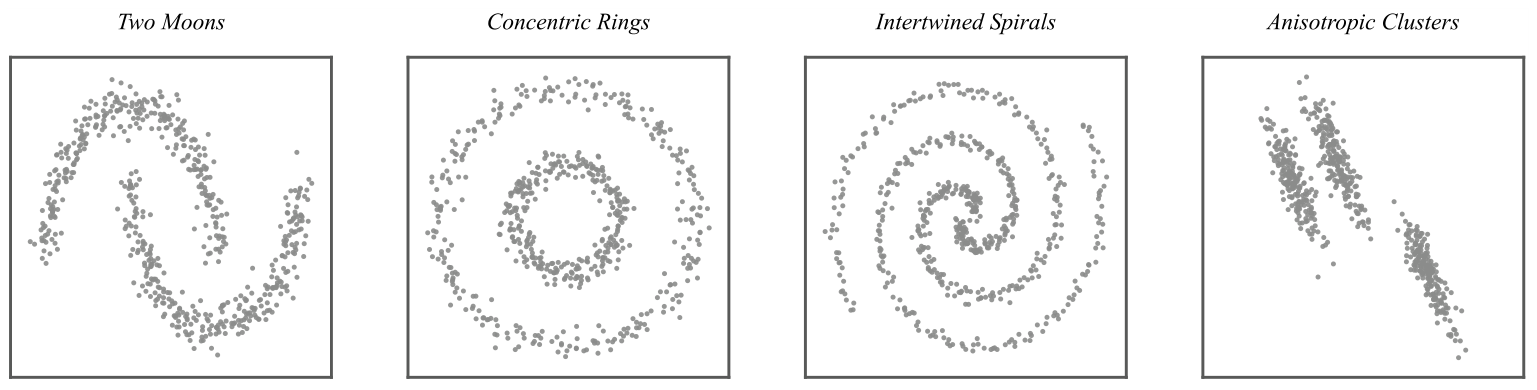
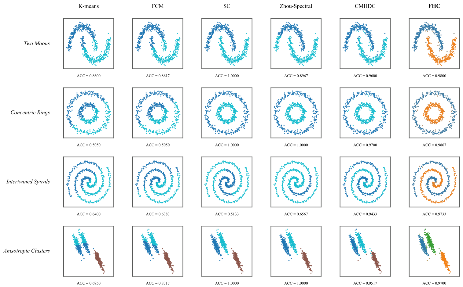
Synthetic datasets are used to examine how the compared methods behave when cluster structure departs from simple prototype-centered geometry. Figure 2 shows four two-dimensional configurations: Two Moons, Concentric Rings, Intertwined Spirals, and Anisotropic Clusters. Each dataset contains 600 standardized samples, and the reference labels are withheld from all clustering algorithms and used only for evaluation and visualization. Figure 3 compares K-means, FCM, SC, Zhou-Spectral, CMHDC, and FHC under this common setting. ACC is shown below each panel, while the blended colors in the FHC results additionally illustrate fuzzy membership uncertainty before maximum-membership assignment.
The overall pattern in Figure 3 is clear. K-means and FCM are less effective on the nested or strongly curved structures, especially Concentric Rings and Intertwined Spirals, whereas methods that exploit relational information recover these structures more successfully. SC and Zhou-Spectral achieve very strong, and in several cases nearly perfect or perfect, partitions, confirming that graph and hypergraph representations are well suited to nonlinear geometry. The differences become more informative on the more difficult configurations. FHC performs particularly well on Intertwined Spirals, where the local structure changes continuously along the two intertwined manifolds and cannot be represented adequately by a small set of prototypes. Its result suggests that organizing neighboring samples into multi-sample relations and evaluating their within-cluster concentration can provide useful information beyond pairwise proximity alone. CMHDC also remains consistently competitive, indicating that adaptive higher-order modeling is beneficial for these data. At the same time, FHC is not uniformly superior on every configuration, which is reasonable because the synthetic datasets emphasize different geometric properties. Overall, the experiment supports the intended role of FHC: its advantage is most evident when local geometry is informative, but the final cluster structure depends on coherent relations among several nearby samples rather than on prototype compactness alone.

5.3. Clustering Performance on Benchmark Datasets

The benchmark comparison is conducted on the thirteen UCI datasets summarized in Table 1, which cover different sample sizes, feature dimensions, and numbers of reference classes. FHC is evaluated against eight representative methods spanning prototype-based, graph-based, deep-clustering, fuzzy-modularity, and hypergraph-clustering paradigms. All methods follow the common protocol described in Section 5.1: the number of clusters is fixed to the reference class number, stochastic methods are repeated for 20 independent runs, and clustering quality is assessed using ACC, NMI, and ARI. This setting provides a broad comparison of conventional baselines and recent deep and higher-order clustering approaches under the same evaluation criteria.
Table 2 shows that FHC achieves the strongest overall ranking across the three evaluation measures. It ranks first in most dataset-metric combinations and remains within the top three in every case, indicating that its advantage is not tied to a single metric or a narrow group of datasets. The gains are especially consistent on several multiclass or structurally more difficult datasets, such as Glass, Image Segmentation, and Optdigits, where FHC performs strongly across ACC, NMI, and ARI. IDC is competitive on several higher-dimensional or larger datasets, including WDBC, Image Segmentation, Waveform, and Optdigits, demonstrating that modern deep representation learning provides a strong additional baseline. CMHDC remains another strong competitor, achieving the best results on Sonar and on selected metrics of WDBC and Page Blocks. These cases show that FHC does not obtain an artificial advantage on every dataset. The relatively small standard deviations further indicate that this performance is maintained across repeated runs.
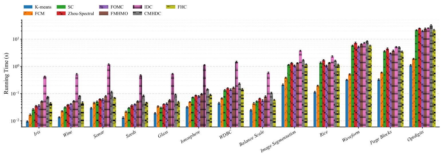
Figure 4 gives a complementary view of computational cost. As expected, K-means and FCM are the fastest methods because they operate directly in the feature space and require little relational construction. IDC introduces a larger fixed computational overhead on the smaller datasets because its deep representation and clustering modules require iterative neural-network training. Graph- and hypergraph-based approaches incur additional costs associated with relation construction, and this difference becomes increasingly visible as dataset size and dimensionality grow. FHC is therefore not intended to compete with the simplest baselines in raw running time. Nevertheless, its total cost remains in the same practical range as the relational competitors and is generally lower than CMHDC, while the sparse edge-wise optimization prevents the higher-order objective from introducing disproportionate overhead. Considering the performance in Table 2 together with the timing results, FHC provides a favorable accuracy-efficiency trade-off: it avoids the iterative representation-learning cost of IDC while retaining higher-order relational modeling, and its additional computational burden remains controlled across the benchmark datasets.

5.4. Statistical Significance Analysis

To determine whether the performance differences reported in Table 2 are statistically significant, we follow the standard multiple-dataset comparison protocol based on the Friedman test followed by the Nemenyi post hoc test [34]. The analysis is based on the mean ACC, NMI, and ARI values reported in Table 2, which are obtained over 20 independent runs for the thirteen benchmark datasets. Because ACC, NMI, and ARI computed on the same dataset are derived from the same clustering results and should not be regarded as independent blocks, the thirteen datasets are treated as independent blocks and separate statistical analyses are conducted for ACC, NMI, and ARI. For each metric, the nine methods are ranked according to their corresponding mean performance on each dataset in Table 2, with rank 1 assigned to the best-performing method. The resulting average ranks are reported in Table 3. For each metric, the Friedman null hypothesis states that all nine methods have equivalent performance across the 13 datasets. Following the standard procedure in [34], the Friedman statistic is converted using the Iman-Davenport correction to obtain an F-distributed statistic F F with 8 and 96 degrees of freedom. At the 0.05 significance level, the corresponding critical value is 2.0363.
As shown in Table 3, FHC obtains the best average rank for all three evaluation measures: 1.2308 for ACC and 1.4615 for both NMI and ARI. CMHDC ranks second for all three metrics, while IDC ranks third. The Iman–Davenport corrected Friedman statistics are F F = 166.4164 for ACC, 174.6258 for NMI, and 194.9388 for ARI. Each statistic is substantially larger than the critical value of 2.0363, with the p-value < 0.001 in all cases. Hence, the null hypothesis that the nine methods perform equivalently is rejected separately for ACC, NMI, and ARI.
After rejecting the three omnibus null hypotheses, separate Nemenyi post hoc tests are conducted according to the same multiple-dataset comparison protocol [34]. For 9 methods and 13 datasets, the critical difference ( C D ) at the 0.05 significance level is C D   =   3.3321 . Table 4 reports the absolute differences between the average rank of FHC and those of each competing method for ACC, NMI, and ARI. A difference larger than the C D indicates that the corresponding pairwise rank difference is statistically significant.

5.5. Ablation Study

To examine the contributions of higher-order relations and data-dependent hyperedge weighting, two reduced variants of FHC are considered. FHC-k2 fixes the hyperedge order at k = 2 , reducing the model to its graph counterpart, while FHC-UW keeps k = 5 but assigns unit weight to all induced hyperedges. Six datasets covering different sample sizes, feature dimensions, and cluster structures are selected. The complete FHC uses exactly the same settings as in Table 2. To maintain consistency with the main benchmark evaluation, the ablation study reports ACC, NMI, and ARI, with all stochastic variants evaluated over the same 20 independent runs.
Table 5 shows a consistent pattern across the three evaluation metrics. The complete FHC achieves the highest mean value on all six datasets for ACC, NMI, and ARI. Averaged over the six datasets, FHC obtains ACC, NMI, and ARI values of 0.7286, 0.5802, and 0.5549, respectively, compared with 0.7170, 0.5692, and 0.5437 for FHC-UW and 0.7045, 0.5573, and 0.5317 for FHC-k2. The larger degradation caused by reducing the hyperedge order to the graph case indicates that explicit multi-sample relational modeling provides the primary contribution to the improvement. FHC-UW consistently performs between FHC-k2 and the complete model, further showing that the data-dependent geometric-mean weighting provides additional discrimination among induced hyperedges. The agreement among ACC, NMI, and ARI confirms that these effects are not limited to label-matching accuracy but are also reflected in information consistency and pairwise partition agreement. Importantly, the complete FHC results in Table 5 are identical to the corresponding ACC, NMI, and ARI values reported in Table 2.

5.6. Parameter Sensitivity

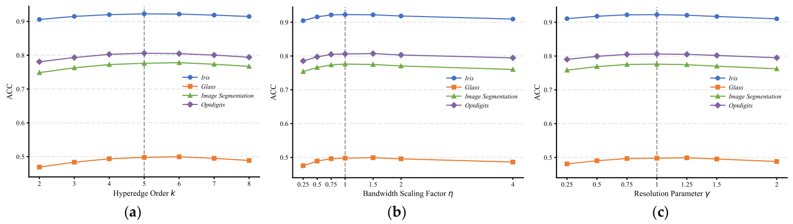
The sensitivity analysis considers the three model-level parameters that directly affect the induced hypergraph or the modularity objective: hyperedge order k , Gaussian bandwidth σ , and resolution parameter γ . To visualize their individual effects without making Figure 5 excessively crowded, four datasets with substantially different characteristics are deliberately selected. Iris represents a small and low-dimensional three-cluster problem; Glass is a small but relatively difficult six-class dataset; Image Segmentation represents a medium-scale multiclass problem; and Optdigits is the largest and highest-dimensional dataset among the selected cases, with ten reference classes. Together, these datasets span markedly different sample sizes, feature dimensions, cluster numbers, and clustering difficulties within the benchmark collection. The tested ranges are k { 2,3 , 4,5 , 6,7 , 8 } , σ = η σ 0 with η { 0.25,0.5,0.75,1 , 1.5,2 , 4 } , where σ 0 is the median pairwise distance, and γ { 0.25,0.5,0.75,1 , 1.25,1.5,2 } . When one parameter is varied, the others are fixed at the default configuration k = 5 , σ = σ 0 , and γ = 1 .
Across the four representative datasets shown in Figure 5, the parameter curves exhibit a relatively stable region around the default configuration rather than a sharply isolated optimum. In particular, the graph reduction k = 2 is generally inferior to moderate higher-order settings, which is consistent with the ablation results in Table 5. Very large hyperedges can slightly reduce performance because increasingly broad neighborhoods may mix samples from different structures. The effects of σ and γ are also moderate around their default values, whereas extreme settings weaken local similarity discrimination or alter the effective clustering resolution. The values at k = 5 , η = 1 , and γ = 1 correspond to the FHC results reported in Table 2. These observations indicate that the default configuration behaves robustly across the four representative settings; a broader quantitative assessment of the joint parameter effect is provided in Appendix A using all thirteen benchmark datasets.
To complement the one-factor-at-a-time analysis in Figure 5 and explicitly examine interactions among the three parameters, we further conduct a joint sensitivity experiment on all thirteen benchmark datasets. Three representative levels around the default configuration are considered for each parameter: k { 3,5 , 7 } , η = σ / σ 0 { 0.5,1.0,1.5 } , and γ { 0.5,1.0,1.5 } . This yields 27 joint parameter configurations. For each configuration, FHC is evaluated using the same 20-run protocol as in Section 5.1, and the mean ACC is first calculated for each dataset and then averaged over all thirteen datasets. The complete quantitative results are reported in Table A1 of Appendix A.
The joint analysis provides a pattern consistent with the individual sensitivity curves. The default configuration k = 5 ,   η = 1 ,   γ = 1 yields an average ACC of 0.7810, while neighboring parameter combinations remain close to this value. For example, with k = 5 and η = 1 , changing γ from 0.5 to 1.5 results in average ACC values between 0.7784 and 0.7810. Across all 27 configurations, the average ACC ranges from 0.7675 to 0.7810. This relatively narrow variation indicates that the default setting lies within a broad high-performing region rather than depending on a narrowly tuned parameter combination, while combinations farther from the central region produce more noticeable performance degradation.

5.7. Convergence and Computational Efficiency

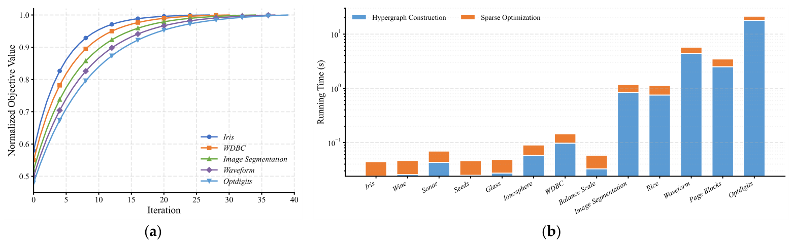
The cross-method running-time comparison has already been reported in Figure 4. This subsection therefore focuses on the internal convergence behavior of FHC and on the distribution of its computational cost between hypergraph construction and sparse modularity optimization. Objective trajectories are recorded on datasets of different scales using the same stopping criterion and Armijo settings as in Section 5.1.
As shown in Figure 6a, the objective increases monotonically and gradually stabilizes, which is consistent with the Armijo-based ascent property established in Section 4. No oscillatory behavior is observed, and the main objective improvement occurs in the early iterations. Figure 6b further shows that the hypergraph-construction stage tends to account for a larger share of the total cost on larger or higher-dimensional datasets, whereas the sparse optimization stage grows more mildly because it operates directly on the stored hyperedges without materializing the high-order tensor.
For consistency, the sum of the construction and optimization times in Figure 6b is the same as the total FHC running time reported in Figure 4 for each dataset. Thus, the efficiency results should be interpreted as a trade-off rather than as a claim that FHC is universally the fastest method: feature-space baselines remain cheaper, while FHC maintains a computational cost in the same practical range as graph- and hypergraph-based methods, with a controlled increase in cost as the dataset size grows.

5.8. Unsupervised Clustering on a Public Alzheimer’s Disease MRI Dataset

To further examine the behavior of FHC beyond conventional tabular benchmarks, we conduct an unsupervised clustering experiment on the public Alzheimer’s Disease Detection Dataset [26]. The dataset contains 6400 brain MRI images in JPG format at a resolution of 256 × 256 pixels and includes four reference categories: NonDemented, VeryMildDemented, MildDemented, and ModerateDemented. After pooling the original training and test folders, the four categories contain 3200, 2240, 896, and 64 images, respectively. The markedly imbalanced distribution makes this dataset substantially more challenging than the tabular benchmarks and provides an application-oriented proof-of-concept setting for evaluating whether higher-order relational clustering can recover group structure that is aligned with the provided reference categories. This experiment is intended as an unsupervised clustering evaluation rather than a clinical validation or diagnostic study.
All images are processed using the label-independent representation described in Section 5.1. Each scan is converted to grayscale and normalized to [ 0,1 ] . Histogram-of-oriented-gradient (HOG) descriptors [27] are extracted using 8 × 8 -pixel cells, 2 × 2 -cell blocks, and nine orientation bins. Principal component analysis (PCA) [28] then reduces the descriptors to 100 dimensions, followed by feature-wise standardization. The same representation is supplied to all methods, and no data augmentation, supervised fine-tuning, label-dependent feature selection, or clinical information is used during clustering.
The same nine clustering methods as in Section 5.3 are compared. The number of clusters is fixed to four for all methods, while the reference category labels remain hidden throughout representation construction and optimization and are used only for external evaluation. FHC uses the default configuration adopted in the benchmark experiments, with hyperedge order k = 5 , Gaussian bandwidth set to the median pairwise Euclidean distance after standardization, and resolution parameter γ = 1 . IDC [32] follows the same deep-clustering implementation and parameter protocol used in the benchmark experiments. For stochastic methods, 20 independent runs are performed using the same random seeds whenever applicable.
Table 6 shows that the feature-space baselines provide relatively limited agreement with the four reference categories, whereas graph-, hypergraph-, and deep-clustering methods generally achieve higher external clustering scores. Among the recent methods, IDC, CMHDC, and FHC form the leading group. IDC attains the highest ACC (0.6342), while FHC achieves the highest NMI (0.3346) and ARI (0.2991) together with the second-best ACC (0.6309). Because the dataset is markedly imbalanced, ACC can be influenced strongly by the dominant NonDemented category, whereas NMI and ARI provide complementary measures of agreement with the overall four-category reference partition. The resulting scores should nevertheless be interpreted as clustering agreement with the dataset labels rather than evidence of clinical discrimination or diagnostic performance.
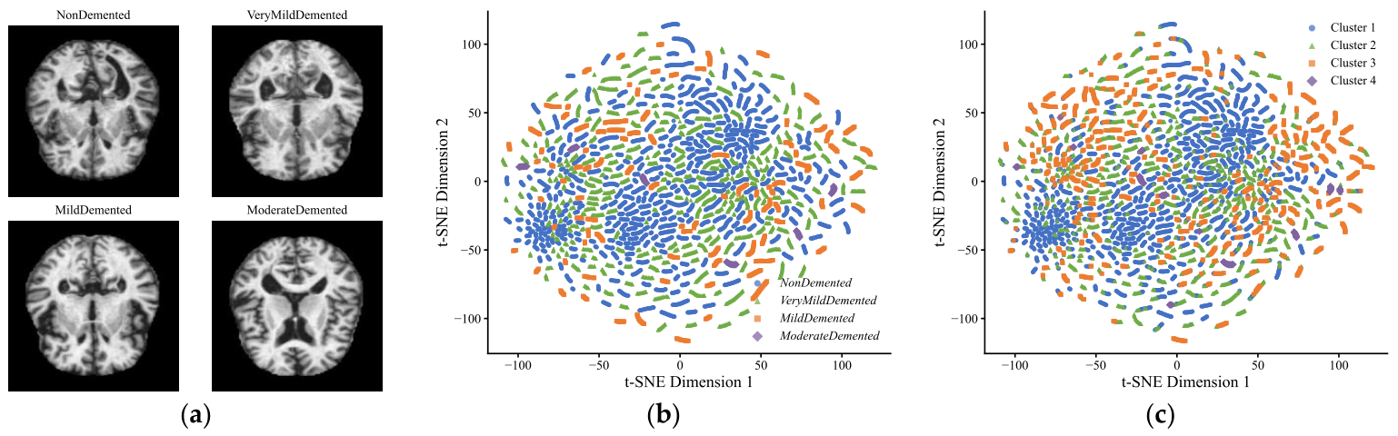
To further examine the clustering behavior at the sample level, Figure 7 provides a visual analysis of the MRI experiment. Representative scans from the four reference categories are first presented to illustrate the image data used in this application. The common 100-dimensional HOG-PCA representation is then projected into two dimensions using t-SNE for visualization only. Importantly, t-SNE is not involved in hypergraph construction or clustering. The same two-dimensional coordinates are used in Figure 7b,c, allowing the reference categories and the cluster assignments to be compared on a point-by-point basis.
The MRI experiment also illustrates the potential role of fuzzy higher-order modeling in a feature space with substantial overlap and severe class imbalance. As visualized in Figure 7, the four reference categories are not sharply separated in the HOG-PCA representation, while the ModerateDemented category contains only a small number of samples. Under such conditions, forcing every observation into a sharply separated prototype-based partition can be restrictive. FHC instead models multi-sample relations through induced hyperedges and retains fuzzy memberships during optimization, allowing ambiguous observations to be represented with graded cluster affiliations before hard labels are obtained for external evaluation. The resulting ACC, NMI, and ARI values remain moderate, which underscores the difficulty of this fully unsupervised clustering task. Nevertheless, the experiment shows that FHC can achieve comparatively strong agreement with the provided reference partition under this feature representation. These results should be regarded as a proof-of-concept clustering evaluation and do not establish clinical validity or diagnostic utility.

6. Discussion

The experiments reveal a consistent pattern. FHC performs particularly well when cluster structure is better described by coherent local relations than by prototype-centered geometry. Across the thirteen benchmark datasets, it achieves the best average rank for ACC, NMI, and ARI. The separate Friedman/Nemenyi analyses show significant advantages over several classical and relational baselines, although the differences from the strongest recent competitors, including IDC, CMHDC, and FMHMO, are not statistically significant. The ablation study further indicates that explicit higher-order relations provide the main performance gain, while data-dependent hyperedge weighting offers an additional benefit. The sensitivity analyses also show that the default configuration lies within a relatively broad high-performing region. From a theoretical perspective, these results support the use of degree-corrected higher-order modularity as a fuzzy clustering criterion. The formulation connects feature-based clustering with relational modularity, reduces to graph-based fuzzy modularity when k = 2 , and further recovers classical Newman–Girvan modularity under hard assignments at unit resolution.
The framework also provides a practical implementation route. Raw observations are first converted into a suitable numerical representation and standardized; local neighborhoods are then organized into weighted hyperedges, with parameters selected using the default configuration or a label-free stability criterion. The sparse hypergraph is subsequently optimized to obtain fuzzy memberships, which may be retained when overlapping or uncertain affiliations are informative or converted into hard labels for conventional clustering analysis. The resulting partition should finally be interpreted and externally validated according to the target domain. For recommendation data, hyperedges may describe local multi-user or multi-item relations and fuzzy memberships may represent overlapping preference groups. For image data, the same workflow can be applied to an appropriate feature representation. The MRI experiment in Section 5.8 illustrates this use only as a proof-of-concept unsupervised clustering evaluation and should not be interpreted as clinical validation.
Several limitations remain. Hypergraph quality depends on neighborhood construction and the global similarity scale, for which stability-based selection, locally scaled similarities, or adaptive neighborhood strategies may provide improvements. Scalability is mainly constrained by pairwise distance calculation and nearest-neighbor search during hypergraph construction; dimensionality reduction, approximate nearest-neighbor search, and anchor-based construction can alleviate this cost. In addition, the nonconvex objective guarantees convergence only to a stationary solution, so multiple or improved initializations may increase reliability. Finally, the number of clusters is assumed to be known, and the input representation is fixed. Automatic cluster-number estimation, nonuniform hypergraphs, and joint representation-hypergraph learning are therefore important directions for future work.

7. Conclusions

This study proposed Fuzzy Hypergraph Clustering (FHC), a higher-order fuzzy clustering framework for ordinary feature data. FHC transforms local neighborhoods into weighted uniform hyperedges and learns fuzzy memberships by maximizing a degree-corrected higher-order modularity objective. The proposed formulation connects higher-order relational modeling with fuzzy clustering while retaining consistency with graph-based fuzzy modularity and classical Newman–Girvan modularity under the corresponding reductions. A projected-gradient ascent algorithm with Armijo backtracking was developed for optimization, and both the objective and gradient can be evaluated directly over sparse hyperedges without explicitly constructing the high-order adjacency tensor.
Experiments on synthetic data, thirteen benchmark datasets, and a public Alzheimer’s MRI dataset support the effectiveness of the proposed framework. FHC achieves consistently strong average ranks across ACC, NMI, and ARI, while the statistical analysis shows that its advantage over the strongest recent competitors is not always statistically significant. The ablation and sensitivity results further support the contribution of higher-order relations and weighted hypergraph construction and indicate that the default parameter configuration is not narrowly tuned. Overall, FHC provides a theoretically consistent and practically implementable alternative for clustering problems in which multi-sample relational structure is important. Future work will focus on adaptive and nonuniform hypergraph construction, more scalable neighborhood generation, improved nonconvex optimization, automatic determination of the number of clusters, and closer integration with learned feature representations.

Author Contributions

Conceptualization, Y.S. and M.W.; methodology, Y.S. and Z.B.; software, Y.S. and E.Z.; validation, Y.S., E.Z. and K.Z.; formal analysis, M.W.; investigation, Y.S.; resources, Z.B.; data curation, Y.S.; writing—original draft preparation, Y.S. and E.Z.; writing—review and editing, M.W. and K.Z.; visualization, M.W.; supervision, K.Z.; project administration, Y.S.; funding acquisition, Y.S., Z.B. and K.Z. All authors have read and agreed to the published version of the manuscript.

Funding

This work was supported in part by the National Natural Science Foundation of China under Grant 62306126, in part by Jiangsu Province Youth Science and Technology Talent Support Project under Grant JSTJ2024283, in part by the Natural Science Foundation of Jiangsu Province (Basic Research Special Fund) under Grant BK20251751, in part by the Natural Science Key Research Projects of Jiangsu Education Department under Grant 22KJA520009 and the Research Project of Jiangsu Vocational College of Information Technology under Grant JSITKY202511.

Data Availability Statement

The benchmark datasets are publicly available from the UCI Machine Learning Repository. The Alzheimer’s disease MRI dataset is publicly available from Mendeley Data as described in Reference [26]. The FHC implementation, synthetic-data generation code, and Alzheimer’s MRI preprocessing scripts are available at https://gitee.com/JNUsyc/fhc (accessed on 10 September 2026).

Conflicts of Interest

The authors declare no conflicts of interest.

Appendix A

Table A1 reports the joint sensitivity results discussed in Section 5.6. For each parameter configuration, the reported value is the ACC averaged over the thirteen benchmark datasets after applying the same 20-run evaluation protocol used in the main experiments. The default configuration is highlighted in bold.
Table A1. Joint sensitivity of k , η = σ / σ 0 , and γ in terms of average ACC over the thirteen benchmark datasets. The default configuration is shown in bold.
k η = σ / σ 0 γ = 0.5 γ = 1.0 γ = 1.5
3 0.5 0.76750.77010.7687
3 1.0 0.77350.77620.7748
3 1.5 0.77080.77360.7720
5 0.5 0.77430.77710.7756
5 1.0 0.77840.78100.7797
5 1.5 0.77620.77880.7775
7 0.5 0.77030.77290.7714
7 1.0 0.77490.77750.7762
7 1.5 0.77270.77530.7739
The highest average ACC is obtained at the default configuration k = 5 ,   η = 1 ,   γ = 1 . However, several neighboring configurations differ by only a few thousandths, confirming that the parameter response around the default setting is relatively smooth. The lowest average ACC occurs at k = 3 ,   η = 0.5 ,   γ = 0.5 , where the combined use of a smaller hyperedge order and a narrower similarity scale reduces the average performance. Overall, the joint results support the qualitative trends shown in Figure 5 and provide a broader robustness check across the complete benchmark set.

References

  1. Liu, X.; Wang, Q.-W.; Chen, J.-F. Multi-View Clustering via Projection-Enhanced Bipartite Graph Learning and Consensus Fusion. Mathematics 2026, 14, 1767. [Google Scholar] [CrossRef] [Scilit]
  2. Li, X.; Yang, H. An End-to-End, Multi-Branch, Feature Fusion-Comparison Deep Clustering Method. Mathematics 2024, 12, 2749. [Google Scholar] [CrossRef] [Scilit]
  3. MacQueen, J. Some methods for classification and analysis of multivariate observations. In Proceedings of the Fifth Berkeley Symposium on Mathematical Statistics and Probability; University of California Press: Berkeley, CA, USA, 1967; Volume 1, pp. 281–297. [Google Scholar]
  4. Bezdek, J.C.; Hathaway, R.J.; Sabin, M.J.; Tucker, W.T. Convergence theory for fuzzy c-means: Counterexamples and repairs. IEEE Trans. Syst. Man Cybern. Syst. 1987, 17, 873–877. [Google Scholar] [CrossRef] [Scilit]
  5. von Luxburg, U. A tutorial on spectral clustering. Stat. Comput. 2007, 17, 395–416. [Google Scholar] [CrossRef] [Scilit]
  6. Zhou, D.; Huang, J.; Schölkopf, B. Learning with hypergraphs: Clustering, classification, and embedding. Adv. Neural Inf. Process. Syst. 2006, 19, 1601–1608. [Google Scholar] [CrossRef] [Scilit]
  7. Agarwal, S.; Branson, K.; Belongie, S. Higher order learning with graphs. In Proceedings of the 23rd International Conference on Machine Learning (ICML 2006), Pittsburgh, PA, USA, 25–29 June 2006; pp. 17–24. [Google Scholar] [CrossRef] [Scilit]
  8. Pelillo, M.; Rota Bulò, S.; Torsello, A.; Albarelli, A.; Rodolà, E. A Game-Theoretic Approach to Pairwise Clustering and Matching. In Advances in Computer Vision and Pattern Recognition; Springer: London, UK, 2013; pp. 179–216. [Google Scholar] [CrossRef] [Scilit]
  9. Shashua, A.; Hazan, T. Non-negative tensor factorization with applications to statistics and computer vision. In Proceedings of the 22nd International Conference on Machine Learning (ICML 2005), Bonn, Germany, 7–11 August 2005; pp. 792–799. [Google Scholar] [CrossRef] [Scilit]
  10. Benson, A.R.; Gleich, D.F.; Leskovec, J. Higher-order organization of complex networks. Science 2016, 353, 163–166. [Google Scholar] [CrossRef] [Scilit]
  11. Newman, M.E.J.; Girvan, M. Finding and evaluating community structure in networks. Phys. Rev. E 2004, 69, 026113. [Google Scholar] [CrossRef] [Scilit]
  12. Reichardt, J.; Bornholdt, S. Statistical mechanics of community detection. Phys. Rev. E 2006, 74, 016110. [Google Scholar] [CrossRef] [Scilit]
  13. Havens, T.C.; Bezdek, J.C.; Leckie, C.; Ramamohanarao, K.; Palaniswami, M. A soft modularity function for detecting fuzzy communities in social networks. IEEE Trans. Fuzzy Syst. 2013, 21, 1170–1175. [Google Scholar] [CrossRef] [Scilit]
  14. Kamiński, B.; Poulin, V.; Prałat, P.; Szufel, P.; Théberge, F. Clustering via hypergraph modularity. PLoS ONE 2019, 14, e0224307. [Google Scholar] [CrossRef] [Scilit]
  15. Kumar, T.; Vaidyanathan, S.; Ananthapadmanabhan, H.; Parthasarathy, S.; Ravindran, B. Hypergraph clustering by iteratively reweighted modularity maximization. Appl. Netw. Sci. 2020, 5, 52. [Google Scholar] [CrossRef] [Scilit]
  16. Sun, Y.; Vong, C.-M.; Wang, S. Fuzzy overlapping modularity clustering for symmetric-tensor based graph. IEEE Trans. Fuzzy Syst. 2025, 33, 3557–3569. [Google Scholar] [CrossRef] [Scilit]
  17. Krishnapuram, R.; Keller, J.M. A possibilistic approach to clustering. IEEE Trans. Fuzzy Syst. 1993, 1, 98–110. [Google Scholar] [CrossRef] [Scilit]
  18. Liu, J.; Chung, F.-L.; Wang, S. Black hole entropic fuzzy clustering. IEEE Trans. Syst. Man Cybern. Syst. 2018, 48, 1622–1636. [Google Scholar] [CrossRef] [Scilit]
  19. Gu, S.; Nojima, Y.; Ishibuchi, H.; Wang, S. Fuzzy style K-plane clustering. IEEE Trans. Fuzzy Syst. 2021, 29, 1518–1532. [Google Scholar] [CrossRef] [Scilit]
  20. Zeng, Y.; Song, P.; Yang, B.; Wang, C.; Du, G.; Yu, Y.; Zheng, W. Hypergraph regularization-based anchor learning for multi-view clustering. Pattern Recognit. 2026, 172, 112465. [Google Scholar] [CrossRef] [Scilit]
  21. Xiao, J.; Ma, Z.-W.; Cao, J.; Xu, X.-K. Hypergraph community detection with fuzzy memberships. IEEE Trans. Fuzzy Syst. 2025, 33, 3253–3266. [Google Scholar] [CrossRef] [Scilit]
  22. Benati, S.; Puerto, J.; Temprano, F. Modularity for hypergraph clustering: Methodologies and applications. Omega 2026, 138, 103387. [Google Scholar] [CrossRef] [Scilit]
  23. Bertsekas, D.P. On the Goldstein-Levitin-Polyak gradient projection method. IEEE Trans. Autom. Control 1976, 21, 174–184. [Google Scholar] [CrossRef] [Scilit]
  24. Condat, L. Fast projection onto the simplex and the ℓ1 ball. Math. Program. 2016, 158, 575–585. [Google Scholar] [CrossRef] [Scilit]
  25. Armijo, L. Minimization of functions having Lipschitz continuous first partial derivatives. Pac. J. Math. 1966, 16, 1–3. [Google Scholar] [CrossRef] [Scilit]
  26. Sufian, A. Advancing Alzheimer’s Disease Detection in Clinical Settings: MRI Image Data; Mendeley Data, Version 1; Elsevier: Amsterdam, The Netherlands, 2025. [Google Scholar] [CrossRef]
  27. Dalal, N.; Triggs, B. Histograms of oriented gradients for human detection. In Proceedings of the 2005 IEEE Computer Society Conference on Computer Vision and Pattern Recognition (CVPR’05), San Diego, CA, USA, 20–25 June 2005; Volume 1, pp. 886–893. [Google Scholar] [CrossRef] [Scilit]
  28. Wan, M.; Wang, X.; Tan, H.; Yang, G. Manifold Regularized Principal Component Analysis Method Using L2,p-Norm. Mathematics 2022, 10, 4603. [Google Scholar] [CrossRef] [Scilit]
  29. Fränti, P.; Sieranoja, S. Clustering accuracy. Appl. Comput. Intell. 2024, 4, 24–44. [Google Scholar] [CrossRef] [Scilit]
  30. Strehl, A.; Ghosh, J. Cluster ensembles—A knowledge reuse framework for combining multiple partitions. J. Mach. Learn. Res. 2002, 3, 583–617. [Google Scholar] [CrossRef][Green Version]
  31. Hubert, L.; Arabie, P. Comparing partitions. J. Classif. 1985, 2, 193–218. [Google Scholar] [CrossRef] [Scilit]
  32. Svirsky, J.; Lindenbaum, O. Interpretable deep clustering for tabular data. In Proceedings of the 41st International Conference on Machine Learning, Vienna, Austria, 21–27 July 2024; Volume 235, pp. 47314–47330. [Google Scholar]
  33. Zhou, Y.; Wu, H.; Hu, J.; Wan, J. Correntropy-induced multi-hypergraph discrete clustering. Signal Process. 2026, 245, 110586. [Google Scholar] [CrossRef] [Scilit]
  34. Demšar, J. Statistical comparisons of classifiers over multiple data sets. J. Mach. Learn. Res. 2006, 7, 1–30. [Google Scholar]
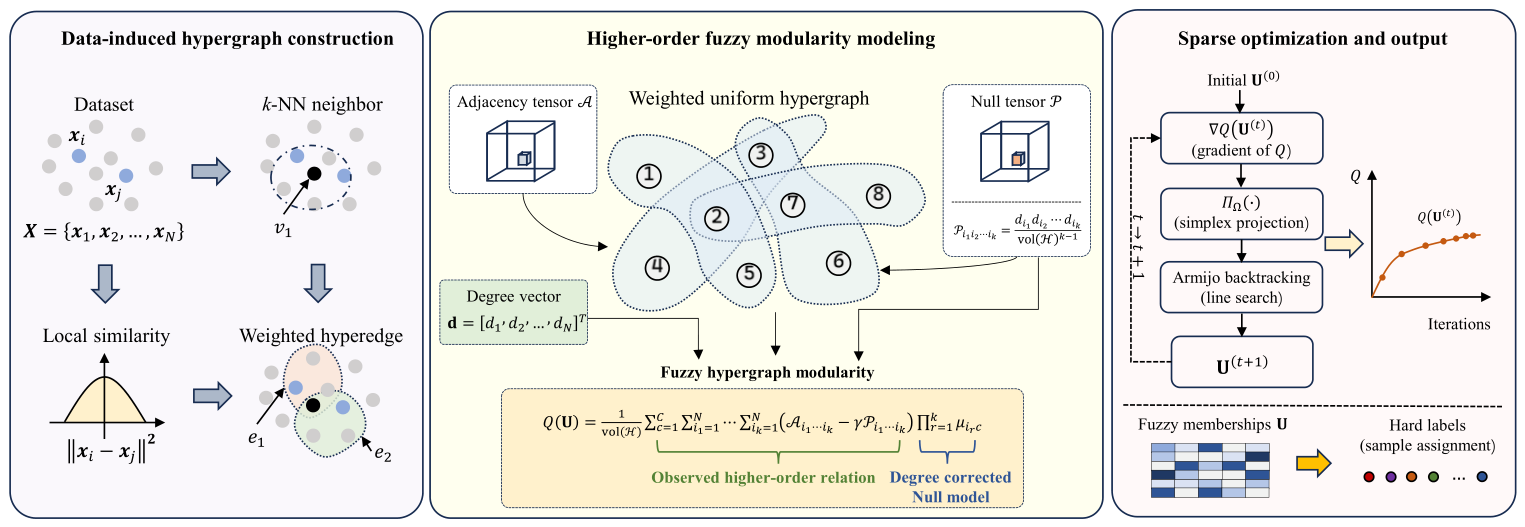
Figure 1. Overall framework of the proposed Fuzzy Hypergraph Clustering (FHC). The three background colors distinguish hypergraph construction, fuzzy modularity modeling, and sparse optimization/output. Circles represent samples or vertices, and shaded regions represent induced hyperedges. Solid arrows indicate forward data/computational flow, dashed arrows indicate iterative feedback, and connecting lines indicate dependencies among model quantities. Mathematical labels and indices identify representative samples, vertices, hyperedges, and iteration states; the colors are used only for visual distinction and have no quantitative meaning.
Mathematics 14 03339 g001
Figure 2. Four representative synthetic datasets used for evaluation. From left to right: Two Moons, Concentric Rings, Intertwined Spirals, and Anisotropic Clusters. All samples are shown in gray to represent the unlabeled inputs provided to the clustering algorithms.
Mathematics 14 03339 g002
Figure 3. Clustering results of six representative methods on the four synthetic datasets. Rows correspond to the datasets and columns to the compared methods. Different colors indicate the cluster assignments produced by each method and are used only to distinguish clusters; the same color does not necessarily represent the same cluster across different methods. ACC is reported below each panel. For FHC, blended colors additionally reflect fuzzy membership confidence before maximum-membership assignment for external evaluation.
Mathematics 14 03339 g003
Figure 4. Running times of the compared clustering methods on the thirteen benchmark datasets.
Mathematics 14 03339 g004
Figure 5. Parameter sensitivity of FHC with respect to (a) hyperedge order k , (b) Gaussian bandwidth scaling factor η , and (c) resolution parameter γ on four representative datasets. The vertical dashed lines indicate the default parameter values used in the main experiments.
Mathematics 14 03339 g005
Figure 6. Convergence and computational behavior of FHC. (a) Normalized fuzzy hypergraph modularity objective versus iteration on representative datasets. (b) Decomposition of FHC running time into hypergraph construction and sparse optimization.
Mathematics 14 03339 g006
Figure 7. Visualization of the Alzheimer’s disease MRI clustering experiment. (a) Representative MRI scans from the four reference categories. (b) t-SNE visualization of the common HOG-PCA representation, with colors indicating the reference categories. (c) Clustering assignments obtained by FHC on the same two-dimensional coordinates.
Mathematics 14 03339 g007
Table 1. Summary of benchmark datasets used in the experiments.
DatasetSamplesFeaturesClasses
Iris15043
Wine178133
Sonar208602
Seeds21073
Glass21496
Ionosphere351342
WDBC569302
Balance Scale62543
Image Segmentation2310197
Rice381072
Waveform5000213
Page Blocks5473105
Optdigits56206410
Table 2. Clustering performance on the thirteen benchmark datasets in terms of ACC, NMI, and ARI. Results are reported as mean ± standard deviation over 20 independent runs. Best mean values are in bold, and second-best mean values are underlined.
DatasetMetricK-MeansFCMSCZhou-
Spectral
FOMCFMHMOIDCCMHDCFHC
IrisACC0.8908 ± 0.00830.8892 ± 0.01000.9067 ± 0.00850.9110 ± 0.00890.9090 ± 0.00700.9200 ± 0.00640.9158 ± 0.00700.9250 ± 0.00630.9225 ± 0.0063
NMI0.7254 ± 0.00940.7431 ± 0.01170.7765 ± 0.01020.7745 ± 0.00900.7915 ± 0.00860.8042 ± 0.00850.8008 ± 0.00890.8160 ± 0.00770.8193 ± 0.0078
ARI0.7148 ± 0.01410.7304 ± 0.01170.7549 ± 0.01080.7716 ± 0.00800.7877 ± 0.00810.7857 ± 0.00730.7950 ± 0.00800.8114 ± 0.00720.8148 ± 0.0070
WineACC0.6910 ± 0.01360.7022 ± 0.01260.7360 ± 0.01150.7538 ± 0.01080.7518 ± 0.00870.7640 ± 0.00840.7685 ± 0.01000.7809 ± 0.00950.7858 ± 0.0101
NMI0.5898 ± 0.01620.5883 ± 0.01540.6342 ± 0.01070.6498 ± 0.01220.6651 ± 0.01100.6747 ± 0.01060.6788 ± 0.01110.6895 ± 0.00930.6955 ± 0.0095
ARI0.4965 ± 0.01570.5112 ± 0.01380.5678 ± 0.01450.5658 ± 0.01200.5937 ± 0.01380.6145 ± 0.01050.6190 ± 0.01150.6301 ± 0.01010.6341 ± 0.0101
SonarACC0.5673 ± 0.02080.5769 ± 0.01790.6140 ± 0.01610.6120 ± 0.01260.6404 ± 0.01460.6384 ± 0.01270.6685 ± 0.01490.6712 ± 0.01390.6668 ± 0.0123
NMI0.0412 ± 0.02160.0478 ± 0.01950.0689 ± 0.01560.0895 ± 0.01540.0875 ± 0.01400.1027 ± 0.01510.1187 ± 0.01610.1209 ± 0.01360.1166 ± 0.0141
ARI0.0215 ± 0.02150.0199 ± 0.02250.0436 ± 0.01890.0562 ± 0.01730.0675 ± 0.01490.0758 ± 0.01520.0898 ± 0.01660.0917 ± 0.01450.0868 ± 0.0141
SeedsACC0.8460 ± 0.01310.8445 ± 0.01180.8762 ± 0.00990.8810 ± 0.00940.8905 ± 0.00830.8952 ± 0.00800.8938 ± 0.00910.9059 ± 0.00850.9126 ± 0.0078
NMI0.6884 ± 0.01300.7042 ± 0.01250.7533 ± 0.01010.7513 ± 0.01090.7735 ± 0.00910.7817 ± 0.00860.7790 ± 0.00980.8048 ± 0.00920.8095 ± 0.0081
ARI0.6517 ± 0.01500.6675 ± 0.01120.7108 ± 0.01200.7333 ± 0.00930.7313 ± 0.00980.7528 ± 0.01100.7480 ± 0.01060.7773 ± 0.00830.7817 ± 0.0092
GlassACC0.3832 ± 0.01590.3925 ± 0.01650.4252 ± 0.01490.4393 ± 0.01410.4636 ± 0.01150.4616 ± 0.01100.4550 ± 0.01240.4953 ± 0.01160.4979 ± 0.0103
NMI0.2998 ± 0.01600.3117 ± 0.01980.3381 ± 0.01600.3544 ± 0.01390.3736 ± 0.01280.3950 ± 0.01580.3890 ± 0.01560.4133 ± 0.01250.4188 ± 0.0134
ARI0.2027 ± 0.02300.2012 ± 0.01790.2500 ± 0.01530.2480 ± 0.01400.2791 ± 0.01330.2926 ± 0.01370.2860 ± 0.01540.3234 ± 0.01430.3285 ± 0.0128
IonosphereACC0.6752 ± 0.01700.6838 ± 0.01220.7151 ± 0.01130.7293 ± 0.01180.7436 ± 0.01120.7521 ± 0.01010.7555 ± 0.01020.7637 ± 0.00880.7707 ± 0.0100
NMI0.2736 ± 0.01740.2857 ± 0.01480.3224 ± 0.01290.3483 ± 0.01320.3463 ± 0.01080.3651 ± 0.01310.3730 ± 0.01260.3890 ± 0.01030.3919 ± 0.0104
ARI0.2987 ± 0.01690.3115 ± 0.01770.3628 ± 0.01350.3608 ± 0.01280.3896 ± 0.01280.4014 ± 0.00990.4110 ± 0.01150.4296 ± 0.01140.4331 ± 0.0093
WDBCACC0.8980 ± 0.01180.8964 ± 0.01210.9272 ± 0.01100.9252 ± 0.00810.9395 ± 0.00730.9375 ± 0.00720.9514 ± 0.00830.9501 ± 0.00810.9526 ± 0.0070
NMI0.5387 ± 0.01190.5512 ± 0.01140.6029 ± 0.01090.6193 ± 0.00830.6318 ± 0.00760.6412 ± 0.00840.6605 ± 0.00870.6637 ± 0.00780.6578 ± 0.0081
ARI0.6215 ± 0.01190.6354 ± 0.01210.6962 ± 0.00960.7221 ± 0.01090.7201 ± 0.00970.7402 ± 0.00900.7645 ± 0.00900.7680 ± 0.00760.7592 ± 0.0079
Balance ScaleACC0.5408 ± 0.01800.5488 ± 0.01820.5744 ± 0.01320.5872 ± 0.01250.5968 ± 0.01150.6114 ± 0.00980.6060 ± 0.01110.6240 ± 0.01030.6270 ± 0.0121
NMI0.1610 ± 0.01740.1595 ± 0.01710.1918 ± 0.01610.2056 ± 0.01260.2182 ± 0.01600.2261 ± 0.01220.2350 ± 0.01290.2478 ± 0.01130.2533 ± 0.0110
ARI0.1458 ± 0.01700.1531 ± 0.01930.1910 ± 0.01630.1890 ± 0.01790.2110 ± 0.01430.2193 ± 0.01240.2290 ± 0.01400.2430 ± 0.01300.2458 ± 0.0129
Image
Segmentation
ACC0.6589 ± 0.01470.6727 ± 0.01410.7121 ± 0.01140.7387 ± 0.01090.7367 ± 0.00960.7545 ± 0.01030.7735 ± 0.01070.7704 ± 0.00970.7762 ± 0.0075
NMI0.6004 ± 0.01760.6156 ± 0.01290.6717 ± 0.01190.6697 ± 0.01410.7050 ± 0.01130.7030 ± 0.01180.7380 ± 0.01150.7369 ± 0.00970.7403 ± 0.0097
ARI0.5583 ± 0.01520.5729 ± 0.01600.6195 ± 0.01350.6427 ± 0.01190.6611 ± 0.01130.6743 ± 0.01180.7060 ± 0.01210.7048 ± 0.01080.7075 ± 0.0084
RiceACC0.8479 ± 0.01150.8464 ± 0.01090.8816 ± 0.00980.8929 ± 0.00930.9016 ± 0.00800.9081 ± 0.01010.9190 ± 0.00890.9218 ± 0.00670.9245 ± 0.0083
NMI0.4631 ± 0.01510.4779 ± 0.01350.5364 ± 0.01250.5697 ± 0.01190.5677 ± 0.01090.6004 ± 0.00930.6200 ± 0.00960.6182 ± 0.00890.6230 ± 0.0095
ARI0.4878 ± 0.01510.5024 ± 0.01530.5764 ± 0.01200.5744 ± 0.01220.6072 ± 0.01060.6209 ± 0.01010.6520 ± 0.00990.6506 ± 0.00860.6558 ± 0.0098
WaveformACC0.5036 ± 0.01450.5124 ± 0.01340.5442 ± 0.01330.5568 ± 0.01260.5758 ± 0.01170.5738 ± 0.01280.5945 ± 0.01180.5933 ± 0.00930.5984 ± 0.0092
NMI0.2504 ± 0.01770.2489 ± 0.01770.2829 ± 0.01440.2974 ± 0.01400.3115 ± 0.01430.3207 ± 0.01310.3460 ± 0.01290.3448 ± 0.01100.3489 ± 0.0096
ARI0.1976 ± 0.01910.2083 ± 0.01720.2389 ± 0.01580.2633 ± 0.01580.2613 ± 0.01340.2798 ± 0.01340.3070 ± 0.01330.3051 ± 0.01140.3102 ± 0.0113
Page BlocksACC0.8535 ± 0.01310.8588 ± 0.01360.8761 ± 0.00950.8845 ± 0.00950.8903 ± 0.00980.8974 ± 0.00840.9060 ± 0.00860.9090 ± 0.00790.9115 ± 0.0067
NMI0.4072 ± 0.01390.4198 ± 0.01190.4641 ± 0.01190.4621 ± 0.01060.4958 ± 0.01080.4938 ± 0.00920.5255 ± 0.00920.5314 ± 0.00810.5212 ± 0.0089
ARI0.3679 ± 0.01360.3796 ± 0.01380.4172 ± 0.01180.4378 ± 0.01030.4559 ± 0.00880.4692 ± 0.01010.4945 ± 0.01000.5010 ± 0.00870.4906 ± 0.0086
OptdigitsACC0.7011 ± 0.01460.6996 ± 0.01350.7415 ± 0.01400.7665 ± 0.01170.7645 ± 0.01070.7819 ± 0.01120.8035 ± 0.01110.8016 ± 0.00980.8060 ± 0.0097
NMI0.6281 ± 0.01400.6425 ± 0.01360.6961 ± 0.01270.6941 ± 0.01130.7201 ± 0.01200.7398 ± 0.01080.7590 ± 0.01180.7568 ± 0.01150.7621 ± 0.0091
ARI0.5958 ± 0.01810.5943 ± 0.01660.6497 ± 0.01210.6755 ± 0.01400.6928 ± 0.01120.7061 ± 0.01060.7325 ± 0.01140.7288 ± 0.01100.7352 ± 0.0119
Table 3. Separate Friedman tests based on the mean ACC, NMI, and ARI results in Table 2 across the thirteen benchmark datasets at significance level = 0.05.
Methods/StatisticACCNMIARI
FHC1.23081.46151.4615
CMHDC2.15382.07692.0769
IDC3.00002.69232.6154
FMHMO4.00003.92313.9231
FOMC4.92315.07695.1538
Zhou-Spectral5.84626.15386.1538
SC6.84626.61546.6154
FCM8.38468.23088.2308
K-means8.61548.76928.7692
F F 166.4164174.6258194.9388
Critical value2.03632.03632.0363
p-value<0.001<0.001<0.001
Null hypothesisRejectedRejectedRejected
Table 4. Nemenyi post hoc comparisons between FHC and the competing methods based on the separate ACC, NMI, and ARI rankings. Significance level = 0.05; C D =   3.3321 . An asterisk indicates a difference exceeding the critical difference.
MethodsACC DifferenceNMI DifferenceARI Difference
CMHDC0.92310.61540.6154
IDC1.76921.23081.1538
FMHMO2.76922.46152.4615
FOMC3.6923 *3.6154 *3.6923 *
Zhou-Spectral4.6154 *4.6923 *4.6923 *
SC5.6154 *5.1538 *5.1538 *
FCM7.1538 *6.7692 *6.7692 *
K-means7.3846 *7.3077 *7.3077 *
Table 5. Ablation results on six representative datasets in terms of ACC, NMI, and ARI. Results are reported as mean ± standard deviation over 20 independent runs. Best mean values are in bold.
DatasetMetricFHC-k2FHC-UWFHC
IrisACC0.9058 ± 0.00840.9147 ± 0.00720.9225 ± 0.0063
NMI0.8015 ± 0.01020.8110 ± 0.00900.8193 ± 0.0078
ARI0.7956 ± 0.00960.8058 ± 0.00840.8148 ± 0.0070
GlassACC0.4692 ± 0.01380.4837 ± 0.01210.4979 ± 0.0103
NMI0.3898 ± 0.01670.4045 ± 0.01510.4188 ± 0.0134
ARI0.3039 ± 0.01610.3163 ± 0.01450.3285 ± 0.0128
IonosphereACC0.7479 ± 0.01280.7594 ± 0.01120.7707 ± 0.0100
NMI0.3780 ± 0.01310.3850 ± 0.01180.3919 ± 0.0104
ARI0.4164 ± 0.01210.4248 ± 0.01070.4331 ± 0.0093
Image
Segmentation
ACC0.7486 ± 0.01060.7629 ± 0.00920.7762 ± 0.0075
NMI0.7087 ± 0.01240.7251 ± 0.01100.7403 ± 0.0097
ARI0.6748 ± 0.01110.6917 ± 0.00970.7075 ± 0.0084
WaveformACC0.5749 ± 0.01210.5871 ± 0.01040.5984 ± 0.0092
NMI0.3325 ± 0.01230.3410 ± 0.01080.3489 ± 0.0096
ARI0.2944 ± 0.01400.3026 ± 0.01240.3102 ± 0.0113
OptdigitsACC0.7808 ± 0.01240.7939 ± 0.01100.8060 ± 0.0097
NMI0.7335 ± 0.01250.7484 ± 0.01100.7621 ± 0.0097
ARI0.7053 ± 0.01410.7209 ± 0.01250.7352 ± 0.0111
AverageACC0.70450.71700.7286
NMI0.55730.56920.5802
ARI0.53170.54370.5549
Table 6. Clustering performance on the Alzheimer’s Disease Detection Dataset. Results are reported as mean ± standard deviation over 20 independent runs. Best mean values are in bold and second-best mean values are underlined.
MethodACCNMIARI
K-means0.5093 ± 0.01480.1824 ± 0.01310.1517 ± 0.0140
FCM0.5168 ± 0.01390.1906 ± 0.01250.1589 ± 0.0132
SC0.5485 ± 0.01270.2261 ± 0.01180.1903 ± 0.0121
Zhou-Spectral0.5612 ± 0.01160.2428 ± 0.01090.2057 ± 0.0114
FOMC0.5756 ± 0.01110.2595 ± 0.01020.2214 ± 0.0108
FMHMO0.5937 ± 0.01040.2809 ± 0.00960.2442 ± 0.0100
IDC0.6342 ± 0.00910.3184 ± 0.00860.2816 ± 0.0088
CMHDC0.6268 ± 0.00900.3239 ± 0.00840.2875 ± 0.0089
FHC0.6309 ± 0.00870.3346 ± 0.00790.2991 ±0.0083
Disclaimer/Publisher’s Note: The statements, opinions and data contained in all publications are solely those of the individual author(s) and contributor(s) and not of MDPI and/or the editor(s). MDPI and/or the editor(s) disclaim responsibility for any injury to people or property resulting from any ideas, methods, instructions or products referred to in the content.