Order-Driven Multi-Objective Optimization of a Three-Echelon Low-Carbon Dairy Cold-Chain Network Considering Demand Variability and Shelf-Life Reliability
Abstract
1. Introduction
- (1)
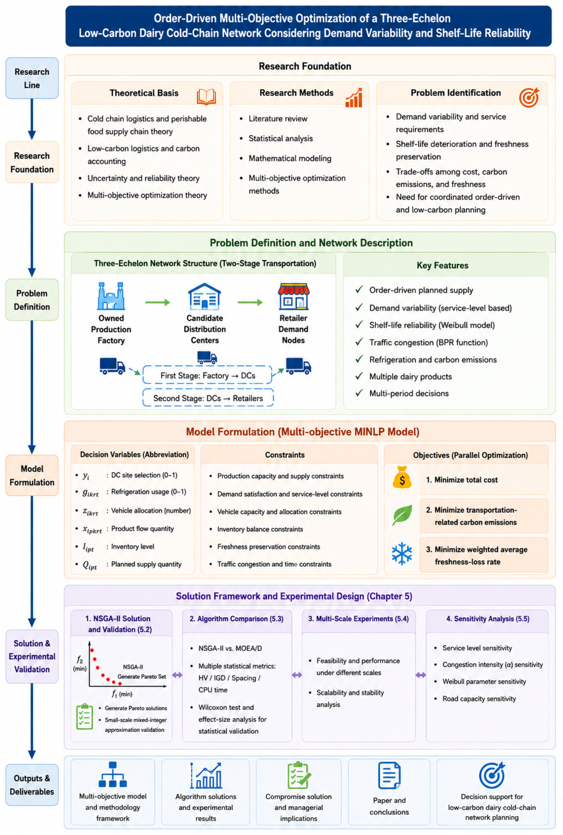
- A three-echelon, two-leg tactical planning model is formulated for the internal production–distribution network of a dairy company. The model jointly coordinates distribution-center location, inventory balance, transportation allocation, vehicle configuration, and refrigeration decisions across multiple products and operational periods. The contribution lies in capturing the interactions among these network and operational decisions within an internal dairy cold-chain setting rather than treating them separately.
- (2)
- An order-driven coordination structure is incorporated to link downstream demand requirements with upstream supply decisions. Demand variability is transformed into service-level-based safe-demand requirements at the retailer level and propagated upstream through distribution allocation and inventory balance to determine planned supply. Accordingly, “order-driven” refers specifically to the downstream-to-upstream transmission of demand information within the network model rather than to a new inventory-balance mechanism or replenishment theory.
- (3)
- Freshness evaluation incorporates both inventory turnover and transportation exposure within the tactical planning framework. Weibull-based shelf-life reliability is combined with time exposure from first-leg transportation, an inventory turnover-based equivalent residence time at distribution centers, and second-leg transportation. This formulation provides a tractable means of capturing the joint effects of inventory and transportation decisions on retail-end freshness without explicitly tracking batch-level inventory-age distributions.
2. Literature Review
2.1. Perishable-Food Supply-Chain Network Design
2.2. Sustainable Supply Chain and Low-Carbon Logistics
2.3. Multi-Objective Optimization Algorithms for Logistics
2.4. Order-Driven Inventory Coordination
2.5. Literature Review Summary
3. Problem Description and Model Construction
3.1. Problem Description
3.2. Model Assumptions
- (1)
- A one-year planning horizon is considered and divided into several representative operational periods, including low-, regular-, and peak-demand periods. The model focuses on tactical operational-period decisions, including production supply, inventory allocation, and distribution planning, rather than daily vehicle routing, customer visit sequences, or detailed delivery scheduling.
- (2)
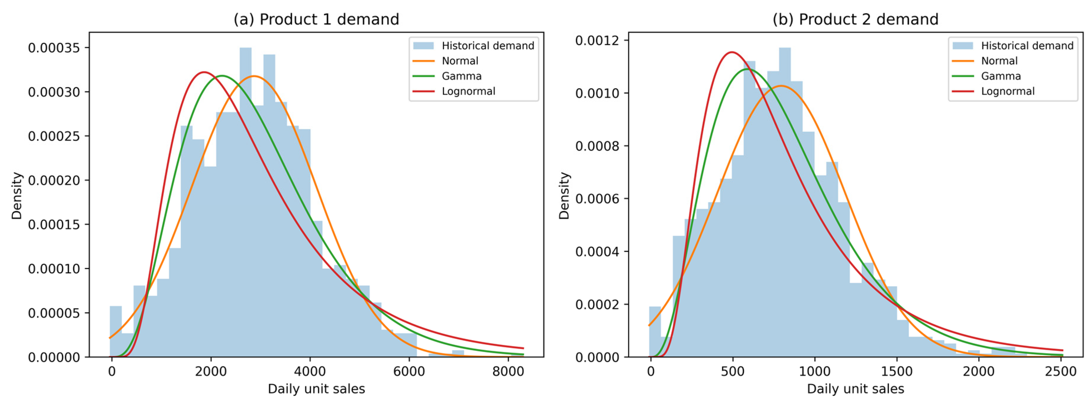
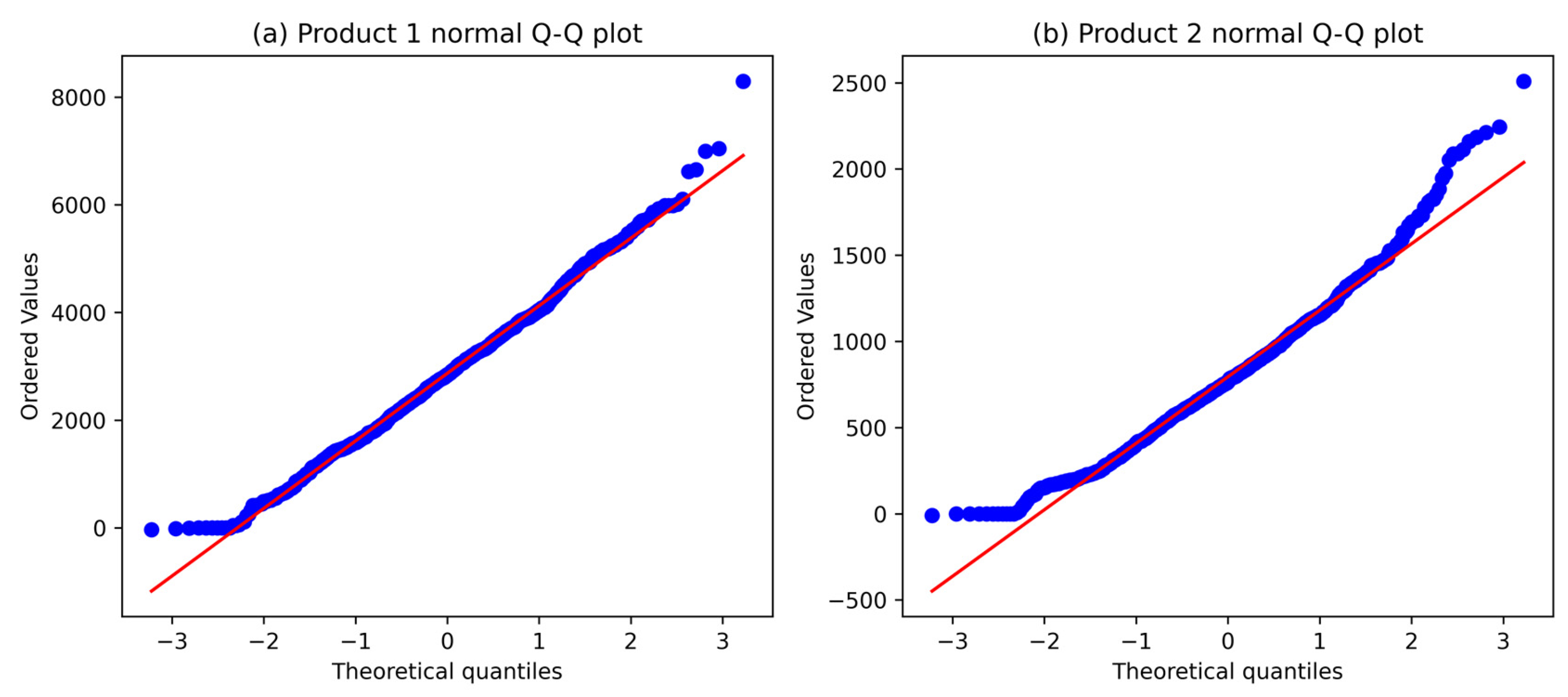
- Retailer demand is characterized as a stochastic variable and is assumed to approximately follow a normal distribution based on the statistical fitting of historical sales data from the Dairy Supply Chain Sales Dataset [31]. The distributional assumption is validated through goodness-of-fit comparisons, as detailed in Appendix A.2. The proposed model further considers independent and weakly correlated demand scenarios to characterize demand variability. The applicability of this representation under different correlation levels is evaluated in Appendix A.8.
- (3)
- To incorporate demand variability while maintaining computational tractability, stochastic demand information is transformed into service-level-based safe-demand requirements using distribution quantiles. Demand risk is controlled ex ante through the selected service-level parameter used to determine safe demand. The resulting safe-demand requirements represent the minimum demand commitment within each operational period and are subsequently treated as deterministic inputs in the optimization model, following previous studies on safe-demand and service-level-based supply-chain planning [26,27].
- (4)
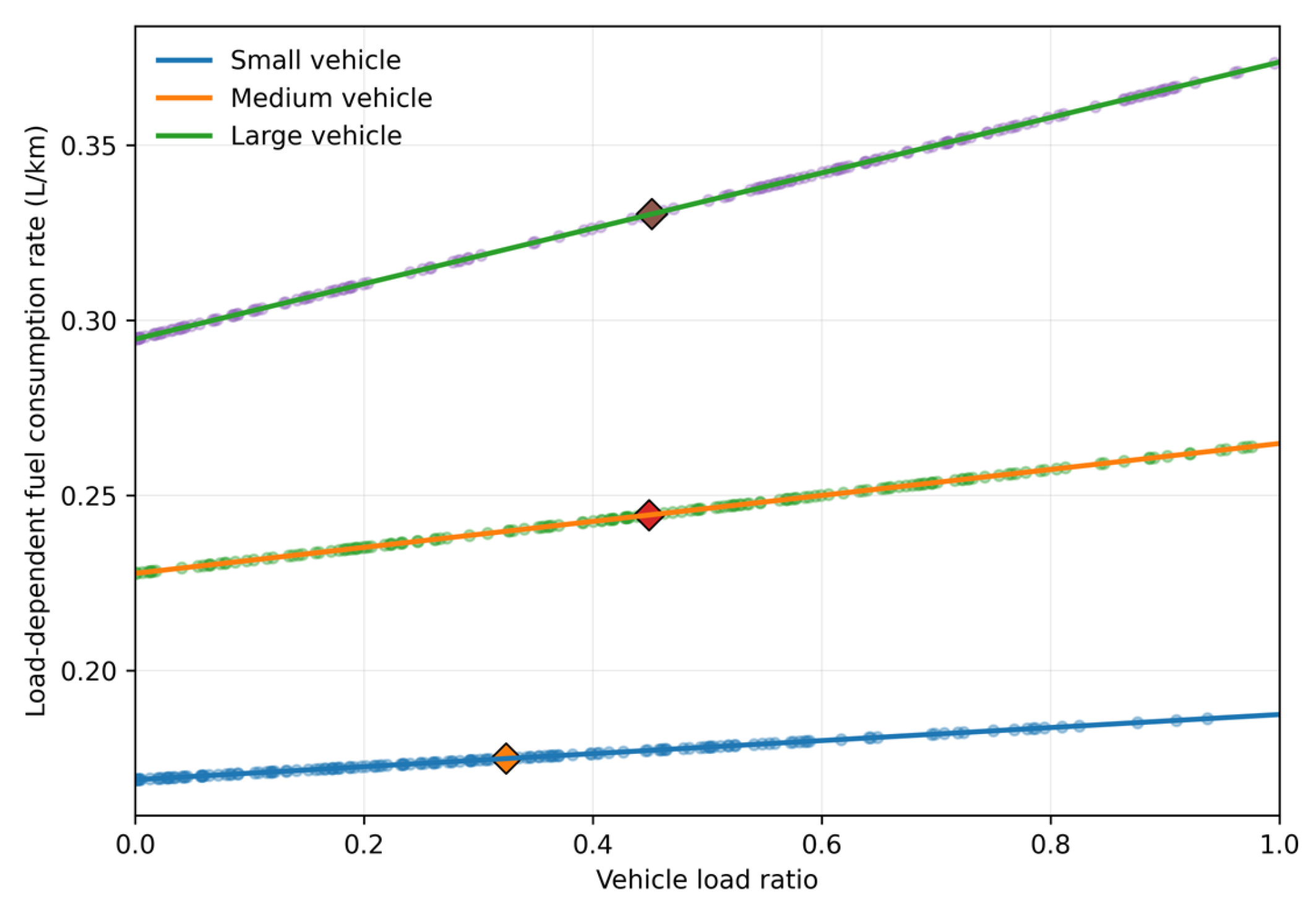
- Unmet demand, backorders, and lost sales are not explicitly considered in the model. Carbon emissions are mainly associated with vehicle fuel consumption and refrigeration energy consumption, which are converted into CO2 emissions using predetermined emission factors. The validity of the adopted transportation fuel-consumption parameters is examined through the validation analysis in Appendix A.4.
- (5)
- The storage-time variable is formulated as an inventory-turnover-based equivalent residence time at the tactical planning level, representing the average storage exposure of products within distribution centers. Freshness evaluation is designed for inventory-age distributions with low to moderate heterogeneity, where average residence time is used to approximate aggregate freshness deterioration. The applicability of this approximation under different inventory-age heterogeneity levels is evaluated in Appendix A.7.
- (6)
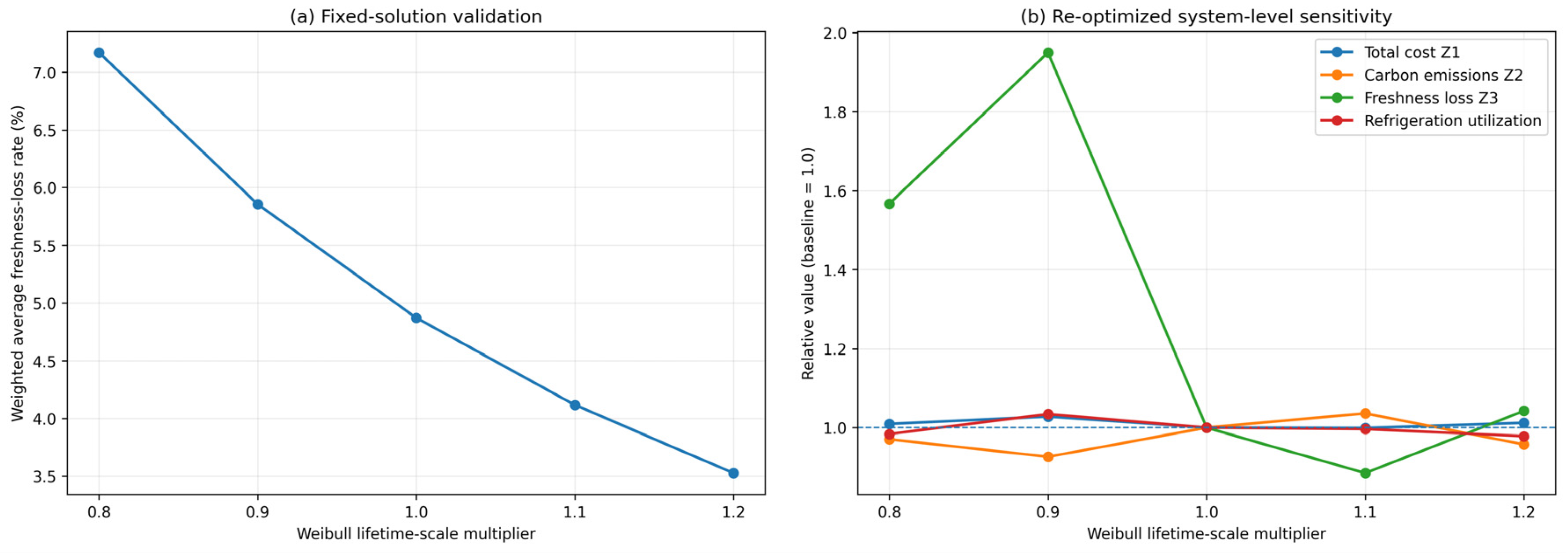
- Product freshness deterioration is characterized using a Weibull-based degradation function under different refrigeration conditions. The Weibull scale and shape parameters are treated as exogenous product-specific characteristics and remain unchanged during optimization. This assumption follows previous perishable-food studies that employ Weibull-type functions to describe shelf-life deterioration and quality degradation behaviors [13]. The Weibull formulation provides a deterministic representation of shelf-life reliability based on cumulative exposure during transportation and storage processes.
- (7)
- Multiple dairy products and vehicle types are considered. Different products may exhibit variations in demand levels, unit weights, and freshness decay characteristics, whereas vehicle types differ in transportation capacity, operating cost, fuel consumption, and refrigeration energy consumption. All vehicles are equipped with refrigeration systems, and refrigeration activation is determined by a binary decision variable. Activating refrigeration enhances freshness preservation but increases energy consumption and transportation-related carbon emissions.
- (8)
- Transportation decisions are modeled at an aggregated tactical level with different representations for the two transportation stages. For first-stage transportation from production facilities to distribution centers, travel time is approximated using representative average speeds without explicitly modeling detailed routes or traffic congestion. Large-capacity vehicles are predefined, and multiple dairy products (e.g., Products A and B) can be jointly transported under refrigerated conditions. For second-stage transportation from distribution centers to retailers, each transportation connection is represented as an aggregated link rather than a specific physical road segment. Travel time is calculated using the BPR function with representative traffic parameters [13,32,33]. Detailed route generation, vehicle scheduling, and multi-stop delivery processes are not considered.
3.3. Symbols and Variables
3.4. Construction of the Basic Model
4. Solution Procedure
4.1. Principles and Mechanisms of the NSGA-II Algorithm
4.2. Entropy-Weight TOPSIS-Based Compromise Solution Selection
5. Numerical Experiments
5.1. Experimental Settings and Data Description
5.2. Analysis and Validation of NSGA-II Solutions
5.3. Comparative Study of NSGA-II and MOEA/D
5.4. Multi-Scale Computational Scalability Analysis
5.5. Sensitivity and Scenario Analysis
6. Conclusions and Future Research
6.1. Conclusions
6.2. Potential Managerial Implications
- (1)
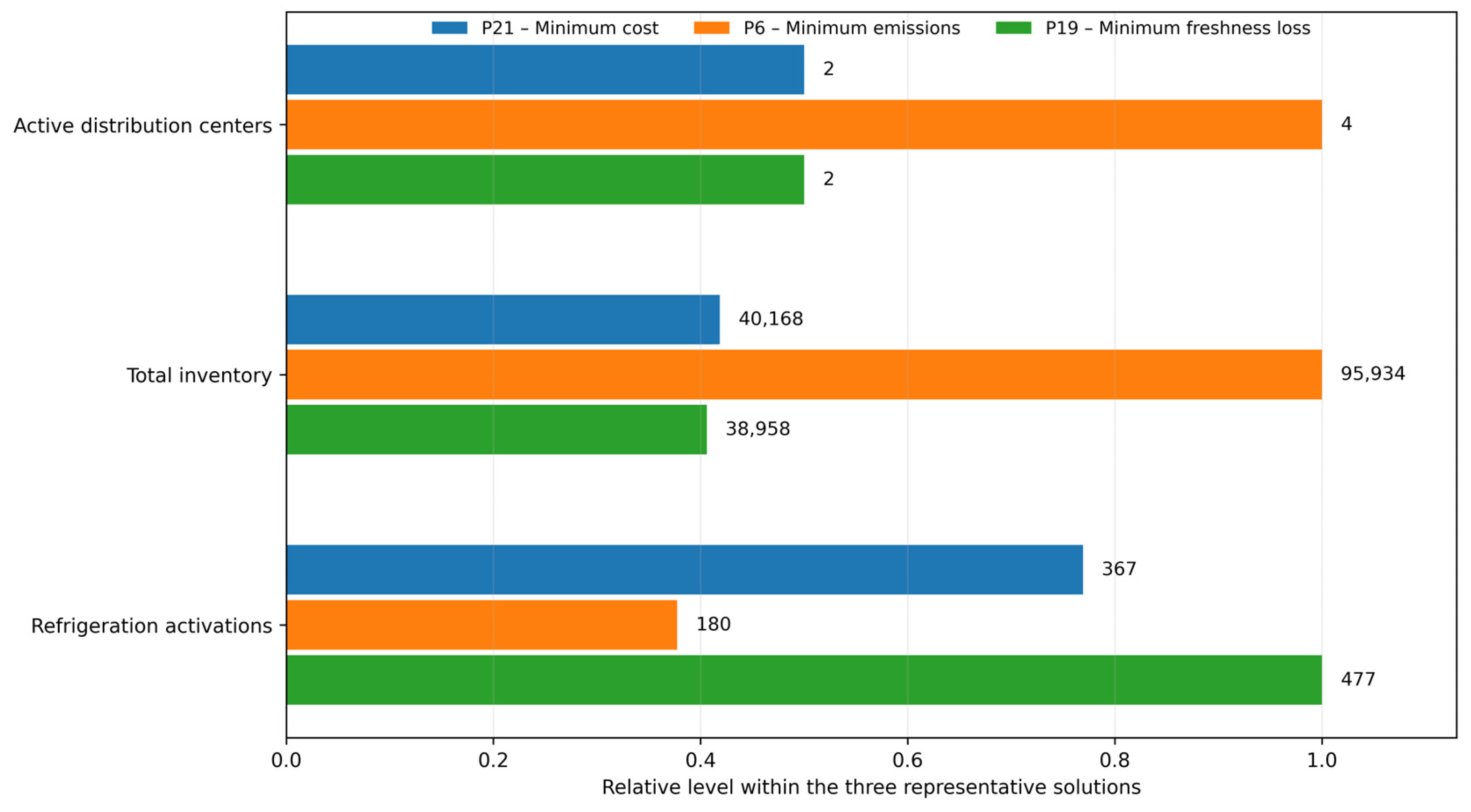
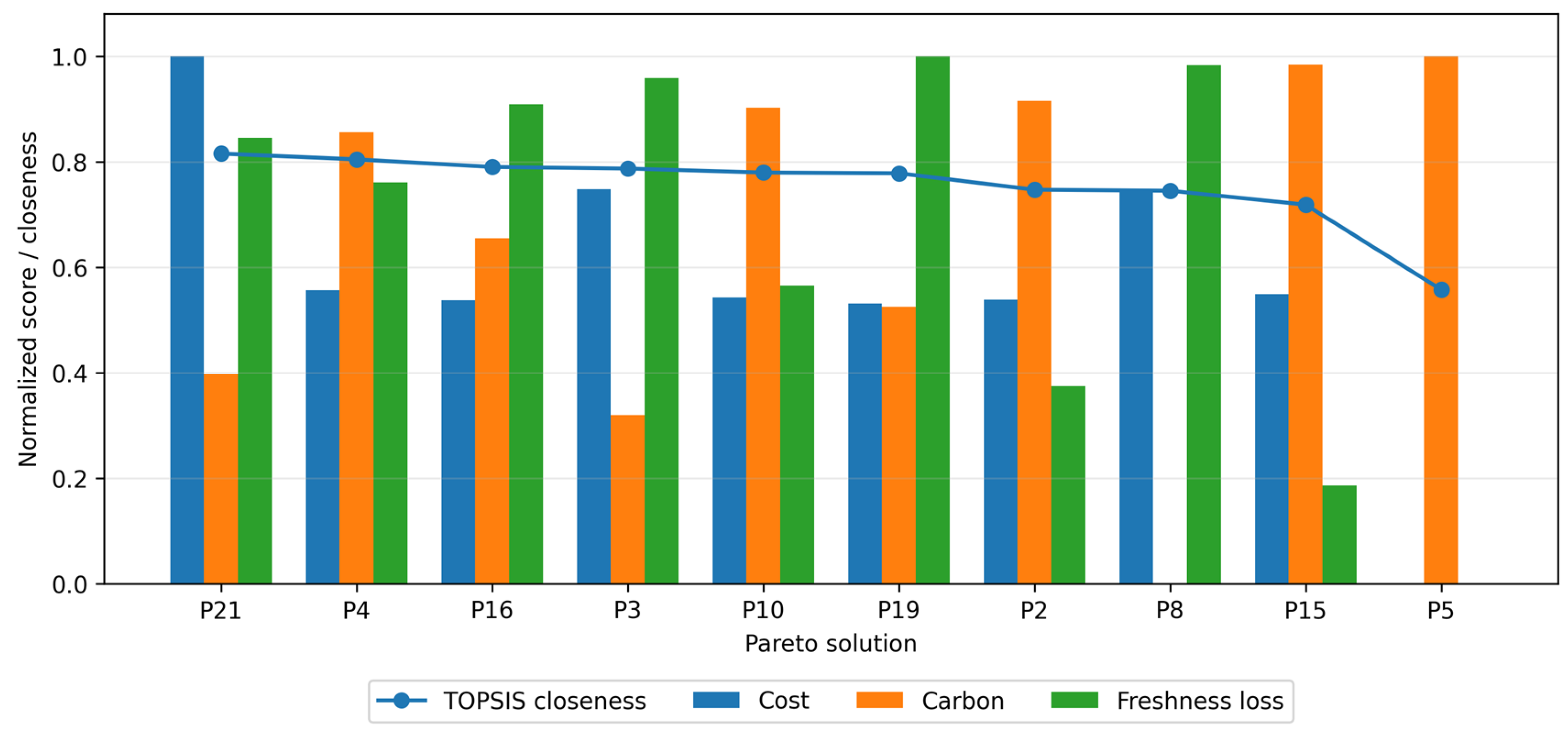
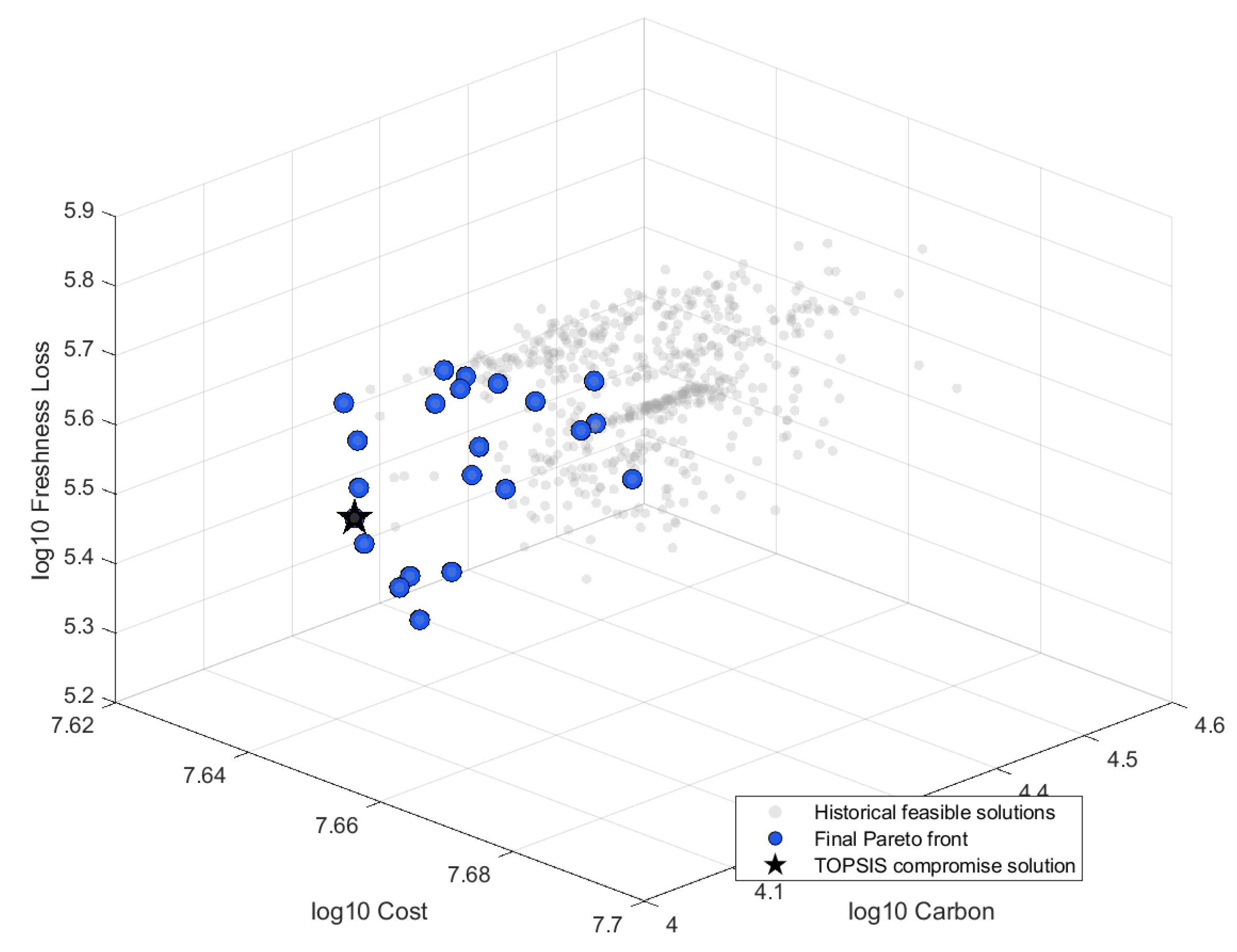
- Multi-objective trade-offs should be explicitly considered in cold-chain planning. The Pareto results show that cost, carbon emissions, and freshness objectives favor different combinations of facility utilization, inventory allocation, transportation, and refrigeration decisions. A cost-oriented plan may therefore compromise environmental or freshness performance. Enterprises can use the Pareto set to compare alternative configurations according to their priorities, while the TOPSIS compromise solution serves as a reference under a specified weighting scheme rather than a universally preferred solution.
- (2)
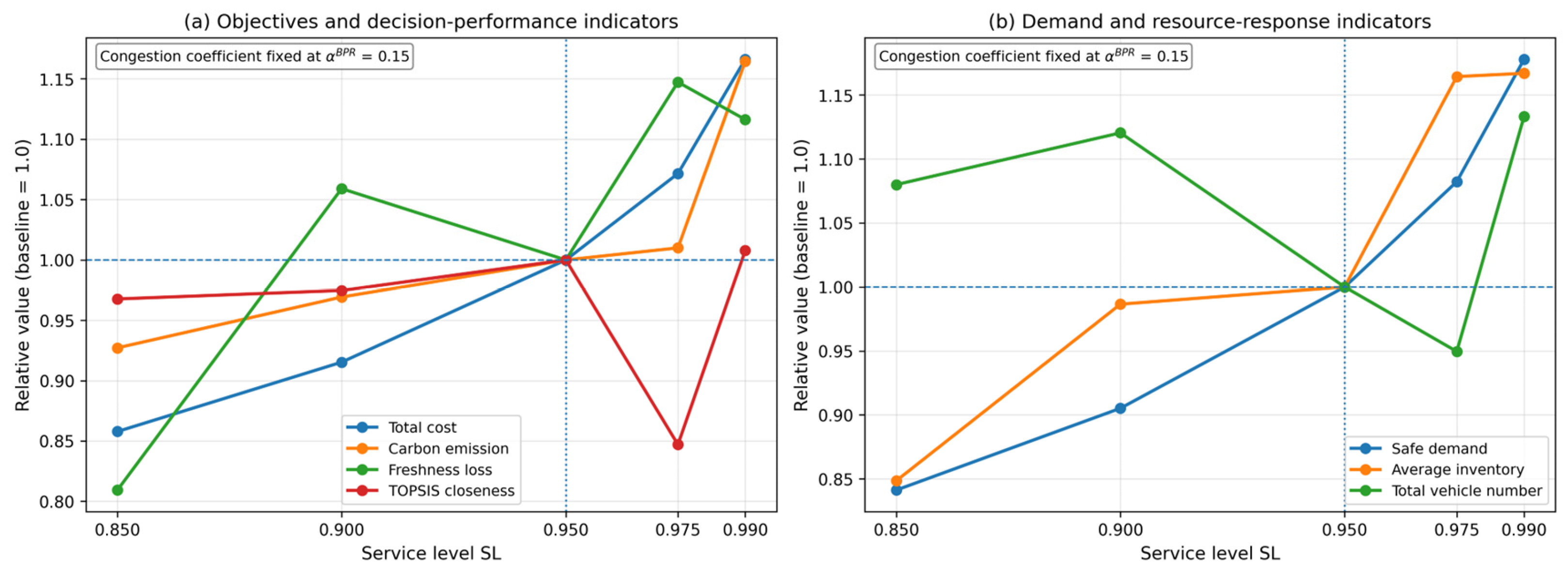
- Service levels should reflect demand and service characteristics. Higher service levels increase safe-demand requirements and consequently affect planned supply, inventory, and resource utilization. Uniformly high service levels may therefore impose unnecessary operating burdens. Enterprises can differentiate service targets across products, customer categories, or operational periods according to demand variability and contractual requirements while considering the associated economic and environmental impacts.
- (3)
- Inventory decisions should balance demand protection and freshness exposure. Additional inventory can support downstream demand fulfillment, but prolonged storage increases freshness deterioration. Tactical planning should therefore emphasize inventory turnover rather than inventory accumulation. Coordinating planned supply, inventory balance, and outbound distribution can reduce unnecessary storage exposure while maintaining adequate demand protection, particularly for products with short or uncertain shelf lives.
- (4)
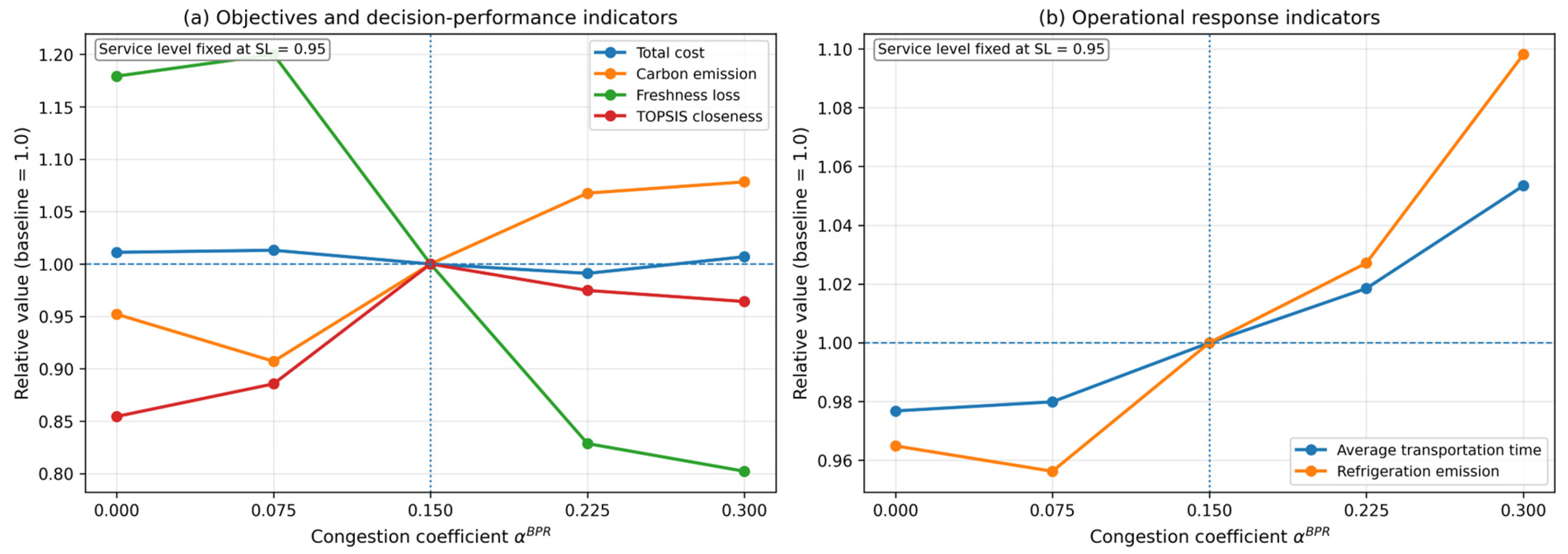
- Transportation capacity and congestion should be incorporated into tactical network planning. Road-capacity scenarios show that transportation conditions affect travel time and, consequently, transportation efficiency, refrigeration operation, emissions, and freshness exposure. Distribution-center utilization and transportation-capacity allocation should therefore reflect major corridor conditions rather than relying solely on nominal distance or uncongested travel time. Detailed routing, vehicle sequencing, and real-time congestion response remain operational-level decisions beyond the scope of the present framework.
- (5)
- Freshness preservation and low-carbon operations should be coordinated. Refrigeration mitigates freshness deterioration but increases energy consumption and associated emissions, while freshness is also influenced by transportation exposure and inventory residence time. Increasing refrigeration intensity alone may therefore be inefficient. Coordinating inventory turnover, transportation conditions, and refrigeration allocation can provide a more balanced means of maintaining freshness while controlling economic and environmental burdens.
6.3. Limitations and Future Research
Author Contributions
Funding
Data Availability Statement
Conflicts of Interest
Appendix A
Appendix A.1. Baseline Case Configuration

| Symbol/Setting | Description | Value |
|---|---|---|
| Candidate distribution centers | 15 | |
| Retailer demand nodes | 60 | |
| Vehicle types | 3 | |
| Product types | 2 | |
| Representative operational periods | 3 | |
| Planning-window length per period | 120 days | |
| Representative first-leg transportation speed | 60 km/h |
Appendix A.2. Demand Data and Distributional Assessment
| Product | Sample Size | Mean Daily Demand | Standard Deviation | CV | Skewness |
|---|---|---|---|---|---|
| Product 1 | 1092 | 2870.13 | 1256.67 | 0.4378 | 0.2465 |
| Product 2 | 1091 | 794.76 | 388.70 | 0.4891 | 0.5675 |
| Product | Distribution | KS Statistic | p-Value | AIC | BIC |
|---|---|---|---|---|---|
| Product 1 | Normal | 0.0211 | 0.7146 | 18,687.47 | 18,697.4 |
| Lognormal | 0.1018 | <0.001 | 18,835.18 | 18,850.1 | |
| Gamma | 0.0702 | <0.001 | 18,569.85 | 18,584.8 | |
| Product 2 | Normal | 0.0374 | 0.0935 | 16,109.98 | 16,119.9 |
| Lognormal | 0.0971 | <0.001 | 16,070.00 | 16,084.9 | |
| Gamma | 0.0579 | 0.0013 | 15,884.66 | 15,899.6 |


Appendix A.3. Cost-Parameter Settings
| Symbol/Code | Value and Unit | Basis |
|---|---|---|
| DC-specific, CNY | Literature-informed [4] | |
| [100, 150, 200], CNY/vehicle | Literature-informed [13] | |
| [1.8, 2.2, 2.5], CNY/(vehicle·km) | Literature-informed [13,21] | |
| [12, 15], CNY/unit | ||
| [0.3, 0.5], CNY/(unit·period) | Literature-informed [4] | |
| [120, 150], CNY/unit | Model setting |
Appendix A.4. Physical, Vehicle, and Capacity Settings
| Symbol/Code | Value | Basis |
|---|---|---|
| Coordinate-based, km | Case calculation | |
| [5980, 8500, 12,000] kg | Case setting | |
| DC-specific | ||
| 1.25 × baseline total safe demand | Baseline calibration | |
| [0.5, 0.8] kg/unit | Case setting | |
| [0.18, 0.25, 0.35] L/km | Literature-informed [6] | |
| [3, 5, 8] kW | Literature-informed [13] |

Appendix A.5. Carbon-Emission and Traffic-Congestion Parameters
| Symbol/Code | Value | Basis |
|---|---|---|
| 2.69 kg CO2/L | Literature-informed [36] | |
| 0.5568 kg CO2/kWh | Literature-informed [37] | |
| , h | Case calculation | |
| 1000 vehicles/h | Scenario setting | |
| [1.0, 1.5, 2.0] | Case setting | |
| 0.15 | Literature-informed [32,33] | |
| 4 |
Appendix A.6. Freshness and Shelf-Life Parameter Settings
| Symbol/Code | Value | Basis |
|---|---|---|
| [0.005, 0.010] | Scenario Settings | |
| [1.2, 1.0] | ||
| [0.18, 0.22] | ||
| [8, 12; 7, 10; 6, 8] days | Scenario setting based on [13,29] | |
| [3, 10; 2.5, 8; 2, 6] days | ||
| 2.0 | ||
| 1.5 | ||
| Small positive value | Numerical setting | |
| Sufficiently large positive value | Logical-constraint setting |
Appendix A.7. Validation of the Average Storage-Time Approximation
Appendix A.7.1. Validation Design and Inventory-Age Scenarios
Appendix A.7.2. Freshness and Objective Re-Evaluation
Appendix A.7.3. Results and Applicability
| Age Distribution | Age CV | |||||||
|---|---|---|---|---|---|---|---|---|
| 0.171 | 0.9340 | 0.9330 | 0.11% | 0.0660 | 0.0670 | 0.10% | 1.49% | |
| 0.382 | 0.9340 | 0.9291 | 0.53% | 0.0660 | 0.0709 | 0.49% | 7.01% | |
| 0.903 | 0.9340 | 0.9065 | 3.04% | 0.0660 | 0.0935 | 2.75% | 29.50% |
Appendix A.8. Out-of-Sample Validation of the Deterministic Quantile Approximation
| Planning Method | Correlation ρ | Empirical Service Level | Expected Shortage | Expected Overage | P95 Total Shortage | P99 Total Shortage | Fill Rate |
|---|---|---|---|---|---|---|---|
| Mean-demand benchmark | 0 | 49.97% | 323,175.74 | 318,240.5 | 367,661.07 | 386,832.40 | 81.69% |
| Quantile-based plan | 0 | 94.98% | 16,920.92 | 1,342,356 | 26,864.73 | 31,786.51 | 99.04% |
| 0.3 | 95.18% | 16,098.54 | 1,350,452 | 67,373.90 | 139,295.17 | 99.08% | |
| 0.6 | 95.34% | 15,439.27 | 1,353,727 | 82,457.90 | 264,347.66 | 99.12% |
Appendix A.9. Sensitivity and Robustness of TOPSIS-Based Compromise Selection
| Test | Setting | Highest-Ranked Solution |
|---|---|---|
| Baseline | Entropy weights + Min–Max normalization | P21 |
| Equal-weight sensitivity | w = (1/3, 1/3, 1/3) | P4 |
| Cost-oriented preference | w = (0.50, 0.25, 0.25) | P4 |
| Carbon-oriented preference | w = (0.25, 0.50, 0.25) | P15 |
| Freshness-oriented preference | w = (0.25, 0.25, 0.50) | P4 |
| Normalization sensitivity | Vector normalization + entropy weights | P16 |
| Run-to-run robustness | 20 independent NSGA-II runs | CV of : 3.67%, 17.40%, 37.38%, |
References
- Aung, M.M.; Chang, Y.S. Temperature management for the quality assurance of a perishable food supply chain. Food Control 2014, 40, 198–207. [Google Scholar] [CrossRef] [Scilit]
- Iyer, P.; Robb, D. Cold chain optimisation models: A systematic literature review. Comput. Ind. Eng. 2025, 204, 110972. [Google Scholar] [CrossRef] [Scilit]
- Musavi, M.; Bozorgi-Amiri, A. A multi-objective sustainable hub location-scheduling problem for perishable food supply chain. Comput. Ind. Eng. 2017, 113, 766–778. [Google Scholar] [CrossRef] [Scilit]
- Biuki, M.; Kazemi, A.; Alinezhad, A. An integrated location-routing-inventory model for sustainable design of a perishable products supply chain network. J. Clean. Prod. 2020, 260, 120842. [Google Scholar] [CrossRef] [Scilit]
- Abdullahi, H.; Reyes-Rubiano, L.; Ouelhadj, D.; Faulin, J.; Juan, A.A. Modelling and multi-criteria analysis of the sustainability dimensions for the green vehicle routing problem. Eur. J. Oper. Res. 2021, 292, 143–154. [Google Scholar] [CrossRef] [Scilit]
- Demir, E.; Bektaş, T.; Laporte, G. A review of recent research on green road freight transportation. Eur. J. Oper. Res. 2014, 237, 775–793. [Google Scholar] [CrossRef] [Scilit]
- Ran, H.; He, D.; Tang, H. Network Optimization of Fresh Products Cold Chain Considering Supply Disruption and Demand Fluctuation Under the Dual-Carbon Policy. Mathematics 2025, 13, 1539. [Google Scholar] [CrossRef] [Scilit]
- Deb, K.; Pratap, A.; Agarwal, S.; Meyarivan, T. A fast and elitist multiobjective genetic algorithm: NSGA-II. IEEE Trans. Evol. Comput. 2002, 6, 182–197. [Google Scholar] [CrossRef] [Scilit]
- Zhang, Q.; Li, H. MOEA/D: A Multiobjective Evolutionary Algorithm Based on Decomposition. IEEE Trans. Evol. Comput. 2007, 11, 712–731. [Google Scholar] [CrossRef] [Scilit]
- Gallego, G.; Özer, Ö. Integrating Replenishment Decisions with Advance Demand Information. Manag. Sci. 2001, 47, 1344–1360. [Google Scholar] [CrossRef] [Scilit]
- Özer, Ö. Replenishment Strategies for Distribution Systems Under Advance Demand Information. Manag. Sci. 2003, 49, 255–272. [Google Scholar] [CrossRef] [Scilit]
- Fisher, M.L. What Is the Right Supply Chain for Your Product? Harv. Bus. Rev. 1997, 75, 105–116. [Google Scholar]
- Jouzdani, J.; Govindan, K. On the sustainable perishable food supply chain network design: A dairy products case to achieve sustainable development goals. J. Clean. Prod. 2021, 278, 123060. [Google Scholar] [CrossRef] [Scilit]
- Shafiee, F.; Kazemi, A.; Jafarnejad Chaghooshi, A.; Sazvar, Z.; Amoozad Mahdiraji, H. A robust multi-objective optimization model for inventory and production management with environmental and social consideration: A real case of dairy industry. J. Clean. Prod. 2021, 294, 126230. [Google Scholar] [CrossRef] [Scilit]
- Behzadi, G.; O’Sullivan, M.J.; Olsen, T.L.; Scrimgeour, F.; Zhang, A. Robust and resilient strategies for managing supply disruptions in an agribusiness supply chain. Int. J. Prod. Econ. 2017, 191, 207–220. [Google Scholar] [CrossRef] [Scilit]
- Sinha, A.K.; Anand, A. Optimizing supply chain network for perishable products using improved bacteria foraging algorithm. Appl. Soft Comput. 2020, 86, 105921. [Google Scholar] [CrossRef] [Scilit]
- Yakavenka, V.; Mallidis, I.; Vlachos, D.; Iakovou, E.; Eleni, Z. Development of a multi-objective model for the design of sustainable supply chains: The case of perishable food products. Ann. Oper. Res. 2020, 294, 593–621. [Google Scholar] [CrossRef] [Scilit]
- Eskandarpour, M.; Dejax, P.; Miemczyk, J.; Péton, O. Sustainable supply chain network design: An optimization-oriented review. Omega 2015, 54, 11–32. [Google Scholar] [CrossRef] [Scilit]
- Govindan, K.; Fattahi, M.; Keyvanshokooh, E. Supply chain network design under uncertainty: A comprehensive review and future research directions. Eur. J. Oper. Res. 2017, 263, 108–141. [Google Scholar] [CrossRef] [Scilit]
- Fang, X.; Nie, L.; Mu, H. Research progress on logistics network optimization under low carbon constraints. IOP Conf. Ser. Earth Environ. Sci. 2020, 615, 012060. [Google Scholar] [CrossRef] [Scilit]
- Thakur, K.; Maity, S.; Nielsen, P.; Pal, T.; Maiti, M. A 3D multiobjective multi-item eco-routing problem for refrigerated fresh products delivery using NSGA-II with hybrid chromosome. Comput. Ind. Eng. 2024, 198, 110644. [Google Scholar] [CrossRef] [Scilit]
- Dai, B.; Chen, H.X.; Li, Y.A.; Zhang, Y.D.; Wang, X.Q.; Deng, Y.M. Inventory replenishment planning of a distribution system with storage capacity constraints and multi-channel order fulfilment. Omega 2021, 102, 102356. [Google Scholar] [CrossRef] [Scilit]
- Melo, M.T.; Nickel, S.; Saldanha-da-Gama, F. Facility Location and Supply Chain Management: A Review. Eur. J. Oper. Res. 2009, 196, 401–412. [Google Scholar] [CrossRef] [Scilit]
- De Kok, T.; Grob, C.; Laumanns, M.; Minner, S.; Rambau, J.; Schade, K. A typology and literature review on stochastic multi-echelon inventory models. Eur. J. Oper. Res. 2018, 269, 955–983. [Google Scholar] [CrossRef] [Scilit]
- Zhang, Y.; Chai, Y.; Ma, L. Research on Multi-Echelon Inventory Optimization for Fresh Products in Supply Chains. Sustainability 2021, 13, 6309. [Google Scholar] [CrossRef] [Scilit]
- Graves, S.C.; Willems, S.P. Optimizing Strategic Safety Stock Placement in Supply Chains. Manuf. Serv. Oper. Manag. 2000, 2, 68–83. [Google Scholar] [CrossRef] [Scilit]
- Trapero, J.R.; Cardós, M.; Kourentzes, N. Quantile forecast optimal combination to enhance safety stock estimation. Int. J. Forecast. 2019, 35, 239–250. [Google Scholar] [CrossRef] [Scilit]
- Cao, Y.; Shen, Z.-J.M. Quantile forecasting and data-driven inventory management under nonstationary demand. Oper. Res. Lett. 2019, 47, 465–472. [Google Scholar] [CrossRef] [Scilit]
- Sel, Ç.; Bilgen, B.; Bloemhof-Ruwaard, J. Planning and scheduling of the make-and-pack dairy production under lifetime uncertainty. Appl. Math. Model. 2017, 51, 129–144. [Google Scholar] [CrossRef] [Scilit]
- Sel, C.; Bilgen, B.; Bloemhof-Ruwaard, J.M.; van der Vorst, J.G.A.J. Multi-bucket optimization for integrated planning and scheduling in the perishable dairy supply chain. Comput. Chem. Eng. 2015, 77, 59–73. [Google Scholar] [CrossRef] [Scilit]
- Iatropoulos, D.; Georgakidis, K.; Siniosoglou, I.; Chaschatzis, C.; Triantafyllou, A.; Liatifis, A.; Pliatsios, D.; Lagkas, T.; Argyriou, V.; Sarigiannidis, P. Dairy Supply Chain Sales Dataset. IEEE Dataport 2023. [Google Scholar] [CrossRef]
- Zhang, J.; Liu, M.; Zhou, B.; Paz, A. Analytical Model for Travel Time-Based BPR Function with Demand Fluctuation and Capacity Degradation. Math. Probl. Eng. 2019, 2019, 5916479. [Google Scholar] [CrossRef] [Scilit]
- United States. Bureau of Public Roads. Traffic Assignment Manual for Application with a Large, High Speed Computer; U.S. Department of Commerce, Bureau of Public Roads, Office of Planning, Urban Planning Division: Washington, DC, USA, 1964. [Google Scholar]
- Little, J.D.C. A Proof for the Queuing Formula: L = lambda W. Oper. Res. 1961, 9, 383–387. [Google Scholar] [CrossRef] [Scilit]
- Wei, L.; Chen, G.; Sun, W.; Li, G. Recognition of Operating Characteristics of Heavy Trucks Based on the Identification of GPS Trajectory Stay Points. Secur. Commun. Netw. 2021, 2021, 9998405. [Google Scholar] [CrossRef] [Scilit]
- U.S. Energy Information Administration. Carbon Dioxide Emissions Coefficients by Fuel. 2024. Available online: https://www.eia.gov/environment/emissions/co2_vol_mass.php (accessed on 25 August 2026).
- Ministry of Ecology and Environment of the People’s Republic of China; National Bureau of Statistics of China. Announcement on the Release of 2021 Electricity Carbon Dioxide Emission Factors; Ministry of Ecology and Environment of the People’s Republic of China: Beijing, China, 2024. [Google Scholar]




| Article | Application | Carbon Emission | Freshness/Quality | Demand Variability | Shelf-Life/ Perishability | Order-Driven Coordination | Refrigeration Decision | Traffic Congestion | Solution Method |
|---|---|---|---|---|---|---|---|---|---|
| Musavi and Bozorgi-Amiri, 2017 [3] | Perishable food | √ | √ | √ | NSGA-II/AUGMECON | ||||
| Biuki et al., 2020 [4] | Perishable products | √ | √ | √ | Hybrid GA/PSO | ||||
| Ran et al., 2025 [7] | Fresh products cold chain | √ | √ | OTS-FICSMA | |||||
| Jouzdani and Govindan, 2021 [13] | Dairy products | △ | √ | √ | √ | RMCGP | |||
| Shafiee et al., 2021 [14] | Dairy supply chain | √ | △ | √ | √ | Heuristic + augmented ε-constraint | |||
| Thakur et al., 2024 [21] | Refrigerated fresh products | √ | √ | √ | √ | NSGA-II with hybrid chromosome | |||
| Dai et al., 2021 [22] | E-commerce distribution inventory | √ | △ | Piecewise linear approximation | |||||
| Zhang et al., 2021 [25] | Fresh products inventory | △ | √ | GA + Flexsim | |||||
| Current Paper | Dairy cold chain logistics | √ | √ | √ | √ | √ | √ | √ | NSGA-II + Entropy- TOPSIS |
| Category | Symbol | Meaning and Explanation |
|---|---|---|
| Set | Set of candidate distribution-center locations, = {1, 2,…, I}, containing all possible locations for establishing a distribution center | |
| Set of retailer locations, = {1, 2,…, R}, containing all retailer locations requiring distribution services | ||
| Set of vehicle types, = {1, 2, 3}, containing three different vehicle types | ||
| Set of product types, = {1, 2}, containing two different types of dairy products | ||
| Set of operating periods, = {1, 2, 3}, representing the low-demand period, regular-demand period, and peak-demand periods | ||
| Computational Variables | The transit time for the first leg of transport from the manufacturing plant to distribution center is calculated as / | |
| The number of vehicles for the first leg of transport from the manufacturing plant to distribution center in period is determined by rounding up the transport weight and vehicle capacity | ||
| The refrigeration status for the first leg of transport from the manufacturing plant to distribution center in period is determined by whether refrigerated product A is being transported | ||
| Congestion-adjusted representative travel time of the aggregate DC -retailer transportation connection in period | ||
| Effective aggregate traffic flow of the DC r -retailer ransportation connection in period, including baseline traffic and the equivalent contribution of logistics vehicles t | ||
| Representative baseline traffic flow of the aggregate transportation connection between DC r and retailer in period | ||
| Inventory-turnover-based equivalent residence time of product at distribution center in period | ||
| Freshness level of product during the first leg of transport from the manufacturing plant to distribution center in period | ||
| Freshness level of product during the second leg of transport from distribution center to retailer via vehicle type in period | ||
| Freshness level of product throughout the entire transportation process in period from the manufacturing plant to distribution center and then to retailer via vehicle type | ||
| Cost Parameters | Fixed facility costs for establishing a distribution center at location | |
| Fixed operating costs for vehicle type (e.g., lease payments, depreciation, etc.) | ||
| Variable cost per unit distance for vehicle type in period | ||
| Unit production and supply cost for product in period | ||
| Unit inventory holding cost for product at distribution center | ||
| Unit disposal cost for the remaining inventory of product at distribution center at the end of the planning period | ||
| Physical Parameters | The first leg of the transport distance from the manufacturing plant to distribution center | |
| The transport distance from distribution center to retailer | ||
| The average speed of all vehicle types | ||
| The maximum load capacity of vehicle type | ||
| The maximum storage capacity of distribution center | ||
| The manufacturing plant’s maximum supply capacity for product in period | ||
| The unit weight of product | ||
| Average fuel-consumption rate per unit distance for vehicle type used in the baseline model | ||
| Carbon Emissions Parameters | Fuel conversion factor: converts fuel consumption into carbon emissions | |
| Electricity conversion factor: converts electricity consumption into carbon emissions | ||
| Representative average refrigeration power of vehicle type | ||
| Required Parameters | Retailer ’s stochastic demand for product in period | |
| The mean and standard deviation of the stochastic demand | ||
| The safe demand at a given service level | ||
| Retailer ’s demand service level for product in period | ||
| The quantile of the standard normal distribution at service level | ||
| Time and Freshness-Related Parameters | Maximum allowable ending inventory of product at distribution center | |
| Shrinkage rate for product during storage at the distribution center | ||
| Maximum acceptable freshness loss rate | ||
| Relative freshness-importance weight of the product | ||
| Travel time from distribution center to retailer under non-congested conditions | ||
| Weibull scale parameter for product during period under refrigerated/non-refrigerated conditions | ||
| Weibull shape parameter for product during period under refrigerated/non-refrigerated conditions | ||
| a planning period length | ||
| Transportation Parameters | Effective traffic capacity of the representative transportation corridor between DC and retailer | |
| Weight of vehicle type in road traffic calculations | ||
| Road congestion intensity coefficient; = 0.15 represents the baseline congestion level | ||
| Exponential parameter of the traffic congestion function (typically set to 4) | ||
| Technical Specifications | A sufficiently large positive number | |
| A very small positive number, to avoid a denominator of 0 | ||
| Objective Function | Economic objective: Minimize the total cost objective function value | |
| Environmental objective: Minimize the transportation -related carbon emissions objective function value | ||
| Quality objective: Quantity- and importance-weighted average freshness-loss rate of delivered products | ||
| Decision Variables | Site selection decision variable: whether to establish a distribution center at location | |
| Refrigeration equipment usage decision: in period , for a trip from distribution center to retailer r using vehicle type , whether to turn on the refrigeration equipment | ||
| Number of vehicles of type used to transport goods from distribution center to retailer in period | ||
| Quantity of product delivered from distribution center to retailer using vehicle type k in period | ||
| Inventory level of product at distribution center in period t | ||
| Estimated supply requirement for product from the manufacturing plant to distribution center in period , driven by projected orders |
| Symbol/Code | Value | Source |
|---|---|---|
| Single NSGA-II: popSize | 100 | Final standalone NSGA-II experiment |
| Single NSGA-II: maxGen | 200 | |
| Algorithm comparison: popSize | 100 | NSGA-II and MOEA/D comparison setting |
| Algorithm comparison: maxGen | 200 | |
| algorithmRepeatTimes | 20 | Independent runs for algorithm comparison |
| Sensitivity analysis: popSize | 80 | Sensitivity and scenario analysis setting |
| Sensitivity analysis: maxGen | 150 | |
| sensitivityRepeatTimes | 5 | Independent runs for each sensitivity scenario |
| crossoverRate | 0.9 | General evolutionary algorithm setting |
| mutationRate | 0.2 | |
| Rng | 20260605 | Fixed random seed for reproducibility |
| Metric | NSGA-II | MOEA/D | p-Value | Effect Size (Cliff’s δ) |
|---|---|---|---|---|
| HV | 0.8512 ± 0.0923 | 0.7461 ± 0.0761 | 0.000622 | 0.675 |
| IGD | 0.1372 ± 0.0392 | 0.1841 ± 0.0409 | 0.000687 | −0.620 |
| Spacing | 0.0724 ± 0.0280 | 0.0735 ± 0.0229 | 0.776391 | −0.025 |
| CPU time (s) | 612.26 ± 35.76 | 2224.27 ± 263.84 | 6.80 × 10⁻⁸ | −1.000 |
| Scale | Network Size (I, R) | Total Safe Demand | Pareto Solutions | HV | CPU Time | |||
|---|---|---|---|---|---|---|---|---|
| Small | (5, 20) | 1,051,728 | 11.80 | 1.2625 | 524.51 | 16,155,984 | 6631.13 | 19.23 |
| Medium | (10, 40) | 1,880,796 | 20.40 | 0.8920 | 716.67 | 25,693,408 | 12,789.10 | 10.19 |
| Large | (15, 60) | 2,843,219 | 29.00 | 1.1172 | 815.49 | 39,419,274 | 14,644.41 | 10.42 |
| Feasible | Mean V/C | Mean Travel Time (h) | ||||
|---|---|---|---|---|---|---|
| 125 | 100% | 0.8289 | 0.61409 | 42,938,937 | 15,135.25 | 0.06515 |
| 250 | 100% | 0.4143 | 0.57026 | 42,744,564 | 15,399.39 | 0.05729 |
| 500 | 100% | 0.2071 | 0.56513 | 42,744,681 | 15,255.48 | 0.05849 |
| 1000 | 100% | 0.1035 | 0.56498 | 42,744,681 | 15,255.29 | 0.05849 |
| 1500 | 100% | 0.0690 | 0.56497 | 42,744,681 | 15,255.28 | 0.05849 |
Disclaimer/Publisher’s Note: The statements, opinions and data contained in all publications are solely those of the individual author(s) and contributor(s) and not of MDPI and/or the editor(s). MDPI and/or the editor(s) disclaim responsibility for any injury to people or property resulting from any ideas, methods, instructions or products referred to in the content. |
© 2026 by the authors. Licensee MDPI, Basel, Switzerland. This article is an open access article distributed under the terms and conditions of the Creative Commons Attribution (CC BY) license.
Share and Cite
Zhang, Y.; Li, Y.; Wu, Y.; Yuan, M.; Li, J. Order-Driven Multi-Objective Optimization of a Three-Echelon Low-Carbon Dairy Cold-Chain Network Considering Demand Variability and Shelf-Life Reliability. Mathematics 2026, 14, 3337. https://doi.org/10.3390/math14183337
Zhang Y, Li Y, Wu Y, Yuan M, Li J. Order-Driven Multi-Objective Optimization of a Three-Echelon Low-Carbon Dairy Cold-Chain Network Considering Demand Variability and Shelf-Life Reliability. Mathematics. 2026; 14(18):3337. https://doi.org/10.3390/math14183337
Chicago/Turabian StyleZhang, Yutong, Yuguo Li, Yiru Wu, Mengyu Yuan, and Jian Li. 2026. "Order-Driven Multi-Objective Optimization of a Three-Echelon Low-Carbon Dairy Cold-Chain Network Considering Demand Variability and Shelf-Life Reliability" Mathematics 14, no. 18: 3337. https://doi.org/10.3390/math14183337
APA StyleZhang, Y., Li, Y., Wu, Y., Yuan, M., & Li, J. (2026). Order-Driven Multi-Objective Optimization of a Three-Echelon Low-Carbon Dairy Cold-Chain Network Considering Demand Variability and Shelf-Life Reliability. Mathematics, 14(18), 3337. https://doi.org/10.3390/math14183337