Finite-n Estimate of Dedekind Numbers Using Layer-Ratio Monte Carlo

Abstract

Dedekind’s problem counts monotone Boolean functions, equivalently downsets of a Boolean lattice. We recast this enumeration as a finite layer-ratio reconstruction problem for the Whitney numbers of the ranked ideal lattice. An exact adjacent-layer double count expresses each layer ratio through local averages of the number of addable elements and the number of removable elements. Reversible fixed-layer Markov chains estimate these averages and hence estimate the Dedekind number $M\left(n\right)$. Backtests at $M\left(8\right)$ and $M\left(9\right)$ calibrate seed-level variability under the fixed protocol and measure the observed Monte Carlo budget scaling. The resulting estimate probes the Whitney-number sequence of the ideal lattice. Although these rows have previously been described empirically as unimodal, the high-precision $n=9$ estimate has a shallow two-shoulder feature around the central rank, contrary to that empirical description; the $n=11$ and $n=13$ center-window estimates show a higher-contrast analogous pattern. The protocol estimate for $M\left(10\right)$ is $\widehat{M}\left(10\right)=(8.9360\pm 0.0010)\times {10}^{78}$, where the displayed uncertainty is the budget-based forecast scale from the cross-n scaling law under the production budget. It is an empirical variability scale associated with the stated Monte Carlo protocol and production budget, estimated from seed-level variation.

1. Introduction

Dedekind’s problem asks for the number $M\left(n\right)$ of monotone Boolean functions on n variables. Equivalently, $M\left(n\right)$ equals each of the following quantities: the number of antichains in the Boolean lattice $B_n={\{0,1\}}^n$ under the coordinatewise order; the number of downsets of $B_n$; and the cardinality of the free distributive lattice on n generators. The problem goes back to Dedekind’s 1897 work on free distributive structures [1]; the free-distributive-lattice and early numerical literature is attributed to Church, Ward, and Yamamoto [2,3,4]. Its elementary formulation hides an extreme computational difficulty: the known exact values currently stop at $n=9$.

The values up to $n=7$ were obtained through a sequence of increasingly refined enumerations [2,3,4]; Wiedemann computed $M\left(8\right)$ in 1991 [5], and later algorithms of Fidytek et al. gave an independent algorithmic confirmation [6]. Subsequent work developed recursive, interval, and downset-enumeration approaches to the same antichain lattice [7,8,9]. A related line of work counts inequivalent monotone Boolean functions and fixed points of variable permutations using Burnside-type reductions [10,11,12,13]. More than three decades after $M\left(8\right)$ was obtained, $M\left(9\right)$ was computed by two independent projects. Jaekel used a matrix formulation together with symmetries of the free distributive lattice and formal concept analysis [14]. Van Hirtum, De Causmaecker and collaborators used a P-coefficient formula, equivalence-class reductions, and FPGA supercomputing [15]; the mathematical form of this computation and its extensions are developed further in [16]. Independent congruence checks for the ninth Dedekind number were also obtained by Pawelski and Szepietowski [17]. Both computations produced

$$M\left(9\right)=286386577668298411128469151667598498812366.$$

Theseexact computations reduce an enormous finite sum by algebraic structure, symmetry, interval decompositions, and specialized hardware. Their primary output is the total $M\left(n\right)$. This should be distinguished from the finer Whitney-number sequence

$$a_n\left(k\right)=\#\{D\subseteq B_n:D\mathrm{is}\mathrm{a}\mathrm{downset}\mathrm{and}|D|=k\},0\le k\le 2^n,$$

where $a_n\left(k\right)$ is the k-th Whitney number of the second kind (or rank number) of $\mathcal{I}\left(B_n\right)$, ranked by ideal cardinality [18], Chapter 3. This sequence records how the total Dedekind number is distributed over the ranks of the ideal lattice. To our knowledge, exact complete rows of this Whitney-number sequence are currently available only through $n=7$ [19]. One advantage of the layer-ratio approach below is that it reconstructs this sequence directly, rather than merely estimating its sum.

The existing exact computations use several concrete reductions. Jäkel’s computation combines matrix enumeration with Formal Concept Analysis and canonical representations of colored graphs to identify (anti-)isomorphic lattice intervals and pairs [14]. The independent computation by Van Hirtum et al. rewrites the P-coefficient formula using equivalence classes and dual-pair deduplication, and evaluates the resulting component-counting workload in parallel on FPGA hardware [15,16]. Recursive algorithms and direct downset enumeration provide further exact approaches at smaller dimensions [6,9]. These methods return certified integer counts. Our layer-ratio method samples fixed-cardinality layers and reconstructs the Whitney-number profile together with its sum. It returns a finite-n numerical estimate whose empirical variability and sampling behavior are evaluated by the stated diagnostics. A detailed comparison of these methods and their outputs is provided in

Table 1. Qualitativecomparison of exact enumeration approaches and the layer-ratio Monte Carlo estimator.

Method	Exactness	Main Output	Computational Feature	Full Whitney Profile
Matrix and interval-symmetry reduction [14]	Exact	Total count	Canonical classification of (anti-)isomorphic intervals and pairs	Not reported
P-coefficients with equivalence classes and FPGA parallelism [15,16]	Exact	Total count and verifiable partial sums	Equivalence-class reduction, dual deduplication, and specialized hardware	Not reported
Recursive/downset enumeration [6,9]	Exact	Total count	Recursive decomposition or direct evaluation of finite posets	Possible when counts are retained by rank
Layer-ratio Monte Carlo	Approximate	Count and layer profile	Budgeted fixed-layer sampling	Directly reconstructed

.

In parallel, a separate line of work involves the asymptotic study of Dedekind’s problem. Kleitman proved that ${\log }_{2}M\left(n\right)$ is asymptotic to the size of the largest layer of the Boolean lattice [20]; the error term was sharpened by Kleitman and Markowsky [21]. Korshunov later obtained asymptotics for $M\left(n\right)$ itself [22,23]. Kahn gave an entropy-based proof of the Kleitman–Markowsky bound through independent sets and antichains [24]; the same independent-set viewpoint also appears in related work on maximal antichains [25]. Korshunov and Shmulevich studied the distribution of monotone Boolean functions by the number of lower units, equivalently the number of terms in the minimal DNF [26]. More recently, cluster-expansion methods from statistical physics have yielded refined asymptotics for Dedekind’s problem and for antichains of prescribed size [27]. These results explain why most of the mass is controlled by the central layers of the Boolean lattice, and they give powerful asymptotic information. Recent work has also developed related variants and generalizations of Dedekind-type counting problems [28,29,30,31,32]. Our objective is to construct a finite-n numerical estimator for values such as $M\left(10\right)$.

We develop a finite-n sampling method that reconstructs the Whitney numbers of the downset lattice. Decompose the set of all downsets by cardinality as follows:

$${\mathsf{\Omega }}_{n,k}=\{D\subseteq B_n:D\mathrm{is}\mathrm{a}\mathrm{downset}\mathrm{and}|D|=k\},a_n\left(k\right)=|{\mathsf{\Omega }}_{n,k}|.$$

Then

$$M\left(n\right)={\displaystyle \sum _{k=0}^{2^n}}{a}_n\left(k\right).$$

Thus, $M\left(n\right)$ is the sum of the finite Whitney-number sequence ${\left(a_n\left(k\right)\right)}_{k=0}^{2^n}$.

For a downset $D\in {\mathsf{\Omega }}_{n,k}$, let $A\left(D\right)$ and $R\left(D\right)$ be the numbers of elements that can be added to or removed from D, respectively, while preserving the downset property. Double-counting cover edges between adjacent layers gives

$$a_n\left(k\right){\mathbb{E}}_{k}A=a_n(k+1){\mathbb{E}}_{k+1}R,{\displaystyle \frac{a_n(k+1)}{a_n\left(k\right)}}={\displaystyle \frac{{\mathbb{E}}_{k}A}{{\mathbb{E}}_{k+1}R}},$$

where ${\mathbb{E}}_k$ denotes expectation under the uniform distribution on ${\mathsf{\Omega }}_{n,k}$. Thus, the global sequence of Whitney numbers can be reconstructed from fixed-layer averages.

Fixed-layer (or microcanonical) Monte Carlo runs a chain on the constrained finite state space with cardinality $|D|=k$ held fixed. The target distribution is uniform on that layer. In the present application, a reversible exchange chain estimates the layer averages of the local boundary statistics A and R. The adjacent-layer double-counting identity converts these averages into the ratio $a_n(k+1)/a_n\left(k\right)$, and accumulation of the ratios recovers the Whitney-number profile. The construction uses the adjacent-layer geometry of the downset lattice.

The layer-ratio construction is related to the broad-histogram approach in statistical mechanics. de Oliveira, Penna, and Herrmann introduced the broad-histogram method for estimating the degeneracy $g\left(E\right)$, the number of microscopic configurations at energy E, from microcanonical averages of local transition multiplicities [33]. de Oliveira subsequently showed that the underlying broad-histogram relation is exact under the appropriate reversibility assumptions [34], namely

$$g\left(E\right){\langle N^{\mathrm{up}}\rangle }_E=g(E+\Delta E){\langle N^{\mathrm{dn}}\rangle }_{E+\Delta E},$$

so that a density-of-states (DOS) ratio is obtained from fixed-energy averages of the numbers of upward and downward moves. In the present combinatorial setting, $a_n\left(k\right)$ is the exact degeneracy of the cardinality shell ${\mathsf{\Omega }}_{n,k}$, ${\mu }_{n,k}$ is its uniform microcanonical analogue, and A and R are the upward and downward local transition multiplicities. Therefore, $a_n\left(k\right){\mathbb{E}}_{k}A=a_n(k+1){\mathbb{E}}_{k+1}R$ has the same double-counting structure, and accumulating its ratios reconstructs the analogue of $\log g$. The correspondence concerns the relation between adjacent shells and local transition counts. In the present setting, k is the downset cardinality coordinate, and the layer measures are uniform on the finite sets ${\mathsf{\Omega }}_{n,k}$.

Conceptually, the ratio step is therefore in the spirit of broad-histogram identities, but here, it is specialized to the fixed-cardinality layers of the downset lattice. General Monte Carlo schemes for finite-set size estimation, such as cascading exclusion [35], follow a different statistical route: the present method uses the adjacent-layer geometry specific to downsets of the Boolean lattice. The main contributions are as follows.

• We formulate Dedekind-number estimation as a finite-n reconstruction problem for the Whitney numbers ${\left(a_n\left(k\right)\right)}_{k=0}^{2^n}$ of the downset lattice, rather than only for the total count $M\left(n\right)$.
• We give a fixed-layer Monte Carlo implementation of the adjacent-ratio estimator together with a log-space reconstruction procedure, validate the resulting estimates at the known values $M\left(8\right)$ and $M\left(9\right)$, and use those cases to calibrate seed-level variability, where a seed means one independent repetition of the fixed protocol.
• We apply the calibrated protocol to estimate $M\left(10\right)$ and analyze the finite-n layer shape, including the two-shoulder structure at $n=9$ and the higher-contrast odd-dimensional center-window patterns at $n=11$ and $n=13$.

The remainder of this paper is organized as follows. Section 2 develops the finite-n layer-ratio framework, including the layer decomposition, the adjacent-layer identity, fixed-layer sampling, deterministic reconstruction, consistency, and the numerical protocol. Section 3 presents the main numerical results, including the known-value validation, the $M\left(10\right)$ estimate, and the reconstructed Whitney-number shapes. Appendix A records the $M\left(10\right)$ production protocol and additional validation diagnostics.

2. Theory and Method

2.1. Layer Decomposition and Ratio Identity

We use the coordinate model of the Boolean lattice, $B_n={\{0,1\}}^n$. Its order is the coordinatewise order. Thus, for $x,y\in B_n$,

$$x⪯y⟺x_i\le y_i\mathrm{for}\mathrm{every}1\le i\le n.$$

We write $x\prec y$ when $x⪯y$ and $x\ne y$.

A subset $D\subseteq B_n$ is a downset if

$$x\in D,y⪯x⟹y\in D.$$

The nth Dedekind number is

$$M\left(n\right)=\#\{D\subseteq B_n:D\mathrm{is}\mathrm{a}\mathrm{downset}\}.$$

Equivalently, $M\left(n\right)$ counts monotone Boolean functions and antichains. Let $N=|B_n|=2^n$. The downsets are ranked by cardinality: for $0\le k\le N$, write

$${\mathsf{\Omega }}_{n,k}=\{D\subseteq B_n:D\mathrm{is}\mathrm{a}\mathrm{downset}\mathrm{and}|D|=k\}$$

and

$$a_n\left(k\right)=|{\mathsf{\Omega }}_{n,k}|.$$

The number $a_n\left(k\right)$ is the k-th Whitney number of the second kind (or rank number) of the ranked ideal lattice $\mathcal{I}\left(B_n\right)$. The sequence $\left(a_n\left(k\right)\right)$ is therefore the Whitney-number sequence of $\mathcal{I}\left(B_n\right)$, and

$$M\left(n\right)={\displaystyle \sum _{k=0}^{2^n}}{a}_n\left(k\right).$$

When n is fixed, we suppress it from the notation when this causes no ambiguity. Let ${\mu }_{n,k}$ be the uniform probability measure on ${\mathsf{\Omega }}_{n,k}$. For any real-valued function $F:{\mathsf{\Omega }}_{n,k}\to \mathbb{R}$, define

$${\mathbb{E}}_{k}F={\displaystyle \frac{1}{a_n\left(k\right)}}\sum _{D\in {\mathsf{\Omega }}_{n,k}}F\left(D\right).$$

For each layer used below, ${\mathsf{\Omega }}_{n,k}$ is a finite nonempty set. We use the power-set sigma algebra ${\mathcal{F}}_{n,k}=2^{{\mathsf{\Omega }}_{n,k}}$ and the uniform probability measure ${\mu }_{n,k}$. Thus, for every $E\in {\mathcal{F}}_{n,k}$, ${\mu }_{n,k}\left(E\right)=|E|/a_n\left(k\right)$ and ${\mu }_{n,k}\left(\left\{D\right\}\right)=1/a_n\left(k\right)$. The displayed expectation is the integral of F with respect to $({\mathsf{\Omega }}_{n,k},{\mathcal{F}}_{n,k},{\mu }_{n,k})$.

Let $W_k\left(\mathcal{I}\left(B_n\right)\right)$ denote the Whitney number of the second kind (the rank number) at rank k. By definition, $W_k\left(\mathcal{I}\left(B_n\right)\right)=a_n\left(k\right)$, and the adjacent-layer ratio is $W_{k+1}/W_k=a_n(k+1)/a_n\left(k\right)$. The notation $W_k$ refers to these second-kind Whitney numbers throughout.

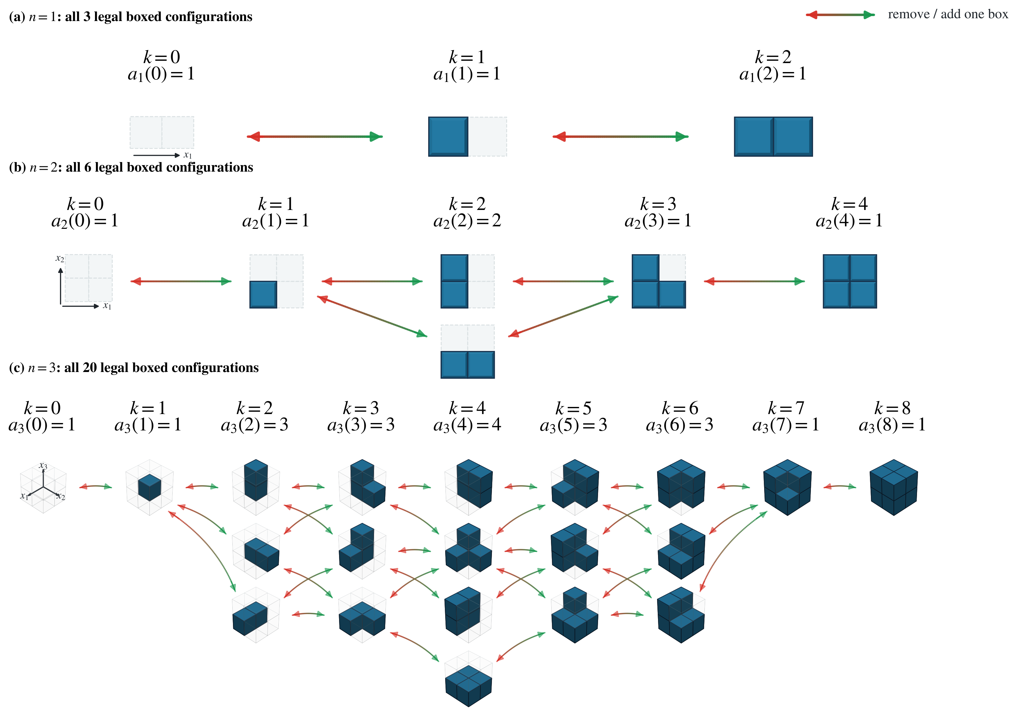
There is a useful boxed-partition viewpoint for these definitions. An n-dimensional partition may be viewed as a finite set of boxes in ${\mathbb{Z}}_{\ge 0}^n$ satisfying the melting rule: whenever a box is present, all coordinatewise smaller boxes are present. This is the box form of MacMahon’s plane partition and higher-dimensional partitions [36,37], using the recent terminology of [38]. Restricting the ambient corner to the $2\times \cdots \times 2$ box ${\{0,1\}}^n$ gives exactly the downsets of $B_n$. Thus, $M\left(n\right)$ is the number of legal boxed configurations in the n-dimensional Boolean box of side length 2, and the Whitney number $a_n\left(k\right)$ counts those configurations with exactly k occupied boxes; see Figure 1.

Intersecting a legal boxed configuration with the finite Boolean box gives a bijection with a downset $D\in {\mathsf{\Omega }}_{n,k}$, where k is the number of occupied boxes. The boxed configurations in the k-box slice are therefore the elements of ${\mathsf{\Omega }}_{n,k}$, and ${\mu }_{n,k}$ assigns mass $1/a_n\left(k\right)$ to each configuration. For any statistic F, ${\mathbb{E}}_{k}F=a_n{\left(k\right)}^{-1}{\sum }_{D\in {\mathsf{\Omega }}_{n,k}}F\left(D\right)$ is the uniform average over the legal boxed configurations with k occupied boxes.

For $D\in {\mathsf{\Omega }}_{n,k}$, let

$$A\left(D\right)=\#\{x\in B_n\setminus D:D\cup \left\{x\right\}\mathrm{is}\mathrm{a}\mathrm{downset}\}$$

and

$$R\left(D\right)=\#\{x\in D:D\setminus \{x\left\}\mathrm{is}\mathrm{a}\mathrm{downset}\right\}.$$

Equivalently,

$$A\left(D\right)=|\min (B_n\setminus D)|,R\left(D\right)=|\max \left(D\right)|,$$

where the minimum and maximum are taken with respect to ⪯.

The global enumeration can now be expressed in terms of cover edges between adjacent cardinality layers. Let

$${\mathcal{E}}_{n,k}=\{(D,\mathsf{\Gamma })\in {\mathsf{\Omega }}_{n,k}\times {\mathsf{\Omega }}_{n,k+1}:D\subseteq \mathsf{\Gamma }\}$$

be the set of cover edges between the two adjacent layers. Since $|\mathsf{\Gamma }|=|D|+1$, every edge has the form $\mathsf{\Gamma }=D\cup \left\{x\right\}$ for a unique element $x\in B_n\setminus D$. Equivalently, x is addable for D, and the same x is removable for $\mathsf{\Gamma }$.

Theorem 1

(Layer-ratio reconstruction). For $0\le k<N=2^n$,

$$a_n\left(k\right){\mathbb{E}}_{k}A=a_n(k+1){\mathbb{E}}_{k+1}R.$$

Consequently,

$${\displaystyle \frac{a_n(k+1)}{a_n\left(k\right)}}={\displaystyle \frac{{\mathbb{E}}_{k}A}{{\mathbb{E}}_{k+1}R}}.$$

If the addable/removable averages ${\mathbb{E}}_{k}A$ and ${\mathbb{E}}_{k}R$ are known for all relevant layers, then the whole Whitney-number sequence is determined by

$$a_n\left(0\right)=1,a_n(k+1)=a_n\left(k\right){\displaystyle \frac{{\mathbb{E}}_{k}A}{{\mathbb{E}}_{k+1}R}}(0\le k<N).$$

Equivalently,

$$a_n\left(k\right)={\displaystyle \prod _{j=0}^{k-1}}{\displaystyle \frac{{\mathbb{E}}_{j}A}{{\mathbb{E}}_{j+1}R}},M\left(n\right)={\displaystyle \sum _{k=0}^N}{a}_n\left(k\right).$$

Proof. 

Fix k with $0\le k<N=2^n$. Each layer ${\mathsf{\Omega }}_{n,r}$, $0\le r\le N$, is nonempty: a linear extension of $B_n$ has an initial segment of every cardinality, and every such initial segment is a downset. Thus, $a_n\left(r\right)=|{\mathsf{\Omega }}_{n,r}|>0$. The set ${\mathcal{E}}_{n,k}$ consists of pairs $(D,\mathsf{\Gamma })$ with $D\in {\mathsf{\Omega }}_{n,k}$, $\mathsf{\Gamma }\in {\mathsf{\Omega }}_{n,k+1}$, and $D\subseteq \mathsf{\Gamma }$. Because $|\mathsf{\Gamma }|=|D|+1$, every such pair has a unique representation

$$\mathsf{\Gamma }=D\cup \left\{x\right\}$$

for some $x\in B_n\setminus D$. The pair belongs to ${\mathcal{E}}_{n,k}$ if and only if $D\cup \left\{x\right\}$ is a downset, which is exactly the condition that x is addable to D. Thus, for a fixed $D\in {\mathsf{\Omega }}_{n,k}$, the map

$$x⟼(D,D\cup \{x\left\}\right)$$

is a bijection from the addable elements of D to the edges in ${\mathcal{E}}_{n,k}$, whose lower endpoint is D. There are $A\left(D\right)$ such edges. Since every edge has exactly one lower endpoint, counting by lower endpoints gives

$$|{\mathcal{E}}_{n,k}|=\sum _{D\in {\mathsf{\Omega }}_{n,k}}A\left(D\right).$$

Now, fix an upper-layer configuration $\mathsf{\Gamma }\in {\mathsf{\Omega }}_{n,k+1}$. If $x\in \mathsf{\Gamma }$ is removable, then $D=\mathsf{\Gamma }\setminus \left\{x\right\}$ is a downset in ${\mathsf{\Omega }}_{n,k}$, and $(D,\mathsf{\Gamma })\in {\mathcal{E}}_{n,k}$. Conversely, every edge ending at $\mathsf{\Gamma }$ is obtained from its unique removed element in this way. Hence, the edges in ${\mathcal{E}}_{n,k}$ whose upper endpoint is $\mathsf{\Gamma }$ are in bijection with the removable elements of $\mathsf{\Gamma }$, and their number is $R\left(\mathsf{\Gamma }\right)$. Counting by upper endpoints therefore gives

$$|{\mathcal{E}}_{n,k}|=\sum _{\mathsf{\Gamma }\in {\mathsf{\Omega }}_{n,k+1}}R\left(\mathsf{\Gamma }\right).$$

The layer measures are uniform, so the definitions of the expectations give

$${\mathbb{E}}_{k}A={\displaystyle \frac{1}{a_n\left(k\right)}}\sum _{D\in {\mathsf{\Omega }}_{n,k}}A\left(D\right),{\mathbb{E}}_{k+1}R={\displaystyle \frac{1}{a_n(k+1)}}\sum _{\mathsf{\Gamma }\in {\mathsf{\Omega }}_{n,k+1}}R\left(\mathsf{\Gamma }\right).$$

Substituting these formulae into the two endpoint counts yields

$$|{\mathcal{E}}_{n,k}|=a_n\left(k\right){\mathbb{E}}_{k}A=a_n(k+1){\mathbb{E}}_{k+1}R.$$

This proves the first assertion. Because $k<N$, every $D\in {\mathsf{\Omega }}_{n,k}$ has at least one addable element: choose a minimal element of the nonempty complement $B_n\setminus D$. Likewise, every nonempty downset $\mathsf{\Gamma }\in {\mathsf{\Omega }}_{n,k+1}$ has a maximal element and hence at least one removable element. Thus, $a_n\left(k\right)>0$ and ${\mathbb{E}}_{k+1}R>0$, and division gives

$${\displaystyle \frac{a_n(k+1)}{a_n\left(k\right)}}={\displaystyle \frac{{\mathbb{E}}_{k}A}{{\mathbb{E}}_{k+1}R}}.$$

Finally, $a_n\left(0\right)=1$. Applying the ratio identity successively for $j=0,\dots ,k-1$ gives, by induction,

$$a_n\left(k\right)={\displaystyle \prod _{j=0}^{k-1}}{\displaystyle \frac{{\mathbb{E}}_{j}A}{{\mathbb{E}}_{j+1}R}}.$$

Summing these layer counts over $k=0,\dots ,N$ gives $M\left(n\right)={\sum }_{k=0}^N{a}_n\left(k\right)$. □

The adjacent-layer identity is a finite-poset analogue of the exact broad-histogram relation: consecutive Whitney-number ratios are obtained from fixed-layer averages of addable and removable element counts, without imposing a parametric model on the sequence $a_n\left(k\right)$ [33,34].

2.2. Fixed-Layer Sampling

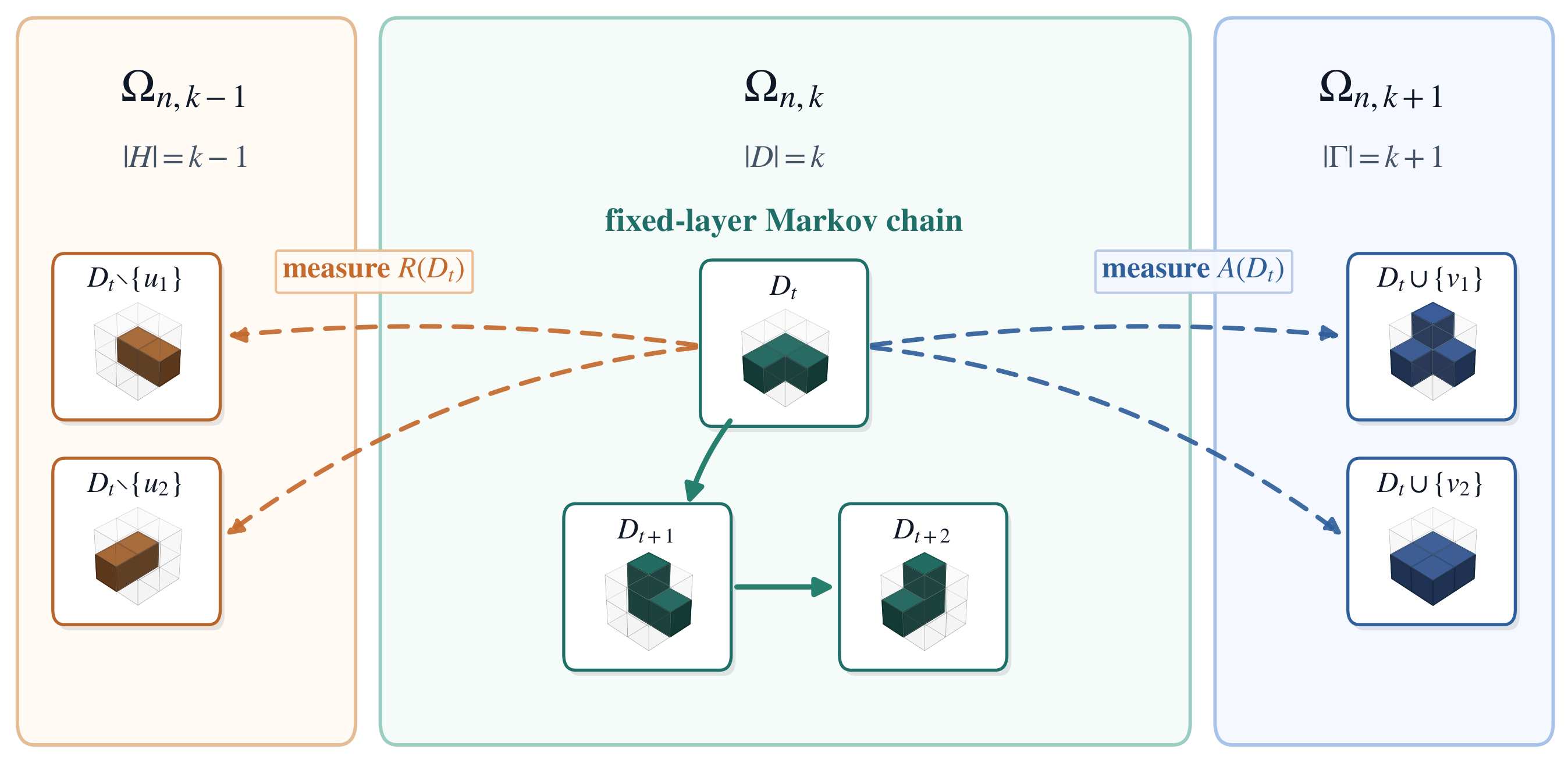
For a fixed n and a fixed layer $0\le k\le N=2^n$, the Markov chain used in this paper has state space ${\mathsf{\Omega }}_{n,k}$. Its purpose is to sample approximately from the uniform layer measure ${\mu }_{n,k}$, so that averages of the addable/removable statistics A and R approximate the microcanonical expectations ${\mathbb{E}}_{k}A$ and ${\mathbb{E}}_{k}R$. The sampling and boundary-measurement mechanism is illustrated in the three-dimensional example in Figure 2.

The elementary move is an exchange move. Starting from a downset $D\in {\mathsf{\Omega }}_{n,k}$, first delete a removable vertex, and then add an addable vertex, as follows:

$$D⟶D^{-}=D\setminus \left\{u\right\}⟶\mathsf{\Gamma }=D^{-}\cup \left\{v\right\}.$$

Here,

$$u\in \max \left(D\right),v\in \min (B_n\setminus D^{-}).$$

By the extremal characterization of addable and removable elements above, deleting u preserves the downset property, and adding v to $D^{-}$ also preserves it. Therefore, $\mathsf{\Gamma }\in {\mathsf{\Omega }}_{n,k}$. If $v=u$, then $\mathsf{\Gamma }=D$, giving a natural self-loop.

The exchange graph $G_{n,k}$ has vertex set ${\mathsf{\Omega }}_{n,k}$, with an edge between two distinct states D and $\mathsf{\Gamma }$ if they differ by deleting one element and adding one element, as above. The Markov chain is a Metropolis–Hastings chain on this graph, with the self-loops coming both from trivial proposals and from rejected nontrivial proposals [39,40].

Assume first that $0<k<N$. Given $D\in {\mathsf{\Omega }}_{n,k}$, the proposal is:

1.

Choose u uniformly from the $R\left(D\right)$ removable vertices of D;

2.

Set $D^{-}=D\setminus \left\{u\right\}$;

3.

Choose v uniformly from the $A\left(D^{-}\right)$ addable vertices of $D^{-}$;

4.

Propose $\mathsf{\Gamma }=D^{-}\cup \left\{v\right\}$.

Fora nontrivial proposal $D\ne \mathsf{\Gamma }$, the removed and added vertices are unique. Write

$$D\setminus \mathsf{\Gamma }=\left\{u\right\},\mathsf{\Gamma }\setminus D=\left\{v\right\},H=D\setminus \left\{u\right\}=\mathsf{\Gamma }\setminus \left\{v\right\}.$$

Then, the proposal probability from D to $\mathsf{\Gamma }$ is

$$q(D,\mathsf{\Gamma })={\displaystyle \frac{1}{R\left(D\right)A\left(H\right)}}.$$

The reverse proposal deletes v from $\mathsf{\Gamma }$ and adds u back to the same intermediate downset H, so

$$q(\mathsf{\Gamma },D)={\displaystyle \frac{1}{R\left(\mathsf{\Gamma }\right)A\left(H\right)}}.$$

The target distribution on ${\mathsf{\Omega }}_{n,k}$ is uniform. Hence, the Metropolis–Hastings acceptance probability for a nontrivial proposal is

$$\alpha (D,\mathsf{\Gamma })=\min \left\{1,{\displaystyle \frac{q(\mathsf{\Gamma },D)}{q(D,\mathsf{\Gamma })}}\right\}=\min \left\{1,{\displaystyle \frac{R\left(D\right)}{R\left(\mathsf{\Gamma }\right)}}\right\}.$$

If the proposal is rejected, the chain remains at D. If $v=u$, the proposal is already D and is treated as an accepted self-loop. The endpoint layers $k=0$ and $k=N$ are singletons, so the chain is the trivial stationary chain there.

Lemma 1

(Stationarity). For each $0\le k\le N$, the uniform distribution ${\mu }_{n,k}$ on ${\mathsf{\Omega }}_{n,k}$ is stationary for the transition kernel described above.

Proof. 

For $k=0$ and $k=N$, the state space is a singleton, so the claim is immediate. Suppose $0<k<N$. It is enough to verify detailed balance for distinct neighboring states $D,\mathsf{\Gamma }\in {\mathsf{\Omega }}_{n,k}$. Since ${\mu }_{n,k}$ is uniform, detailed balance reduces to

$$q(D,\mathsf{\Gamma })\alpha (D,\mathsf{\Gamma })=q(\mathsf{\Gamma },D)\alpha (\mathsf{\Gamma },D).$$

Using the formula above, with $H=D\cap \mathsf{\Gamma }$, the left-hand side is

$${\displaystyle \frac{1}{R\left(D\right)A\left(H\right)}}\min \left\{1,{\displaystyle \frac{R\left(D\right)}{R\left(\mathsf{\Gamma }\right)}}\right\}={\displaystyle \frac{1}{A\left(H\right)\max \left\{R\right(D),R(\mathsf{\Gamma }\left)\right\}}}.$$

The same expression is obtained after exchanging D and $\mathsf{\Gamma }$. Hence, detailed balance holds for every off-diagonal transition. The diagonal terms then balance automatically because each row of the transition matrix sums to one. Therefore, ${\mu }_{n,k}$ is stationary. □

Lemma 2

(Connectivity of fixed layers). For every $0\le k\le N$, the exchange graph $G_{n,k}$ is connected.

Proof. 

The cases $k=0$ and $k=N$ are trivial. Let $0<k<N$, and take two states $D,E\in {\mathsf{\Omega }}_{n,k}$. If $D=E$, there is nothing to prove.

Assume $D\ne E$. Choose an element u maximal in $D\setminus E$ with respect to ⪯. Then, u is also maximal in D. Indeed, suppose that there exists $z\in D$ strictly above u, that is, $u\prec z$. If $z\notin E$, then $z\in D\setminus E$, contradicting the maximality of u in $D\setminus E$. If $z\in E$, then the downset property of E, together with $u\prec z$, implies $u\in E$, again a contradiction. Hence, $u\in \max \left(D\right)$, so deleting u preserves the downset property.

Next, choose an element v minimal in $E\setminus D$, again with respect to ⪯. We claim that v is addable to $D^{-}:=D\setminus \left\{u\right\}$. Let $y\prec v$. Since $v\in E$ and E is a downset, we have $y\in E$. If $y\notin D$, then $y\in E\setminus D$, contradicting the minimality of v. Thus, every $y\prec v$ lies in D. Moreover, $y\ne u$: if $y=u$, then $u\prec v$ and $v\in E$ would imply $u\in E$, contradicting $u\in D\setminus E$. Therefore, every $y\prec v$ lies in $D^{-}$, so $D^{-}\cup \left\{v\right\}$ is a downset.

Thus,

$$D^{\prime }=(D\setminus \left\{u\right\})\cup \left\{v\right\}$$

is a legal exchange move in $G_{n,k}$. Since $u\in D\setminus E$ is removed and $v\in E\setminus D$ is added, we have

$$|D^{\prime }\setminus E|=|D\setminus E|-1.$$

Repeating the same argument finitely many times reaches E. Hence, every two states in ${\mathsf{\Omega }}_{n,k}$ are connected by legal exchange moves, so $G_{n,k}$ is connected. □

Proposition 1

(Ergodicity of the fixed-layer chain). For every $0\le k\le N$, the fixed-layer chain is irreducible and aperiodic. Consequently, for a fixed n and k, the empirical averages of A and R along the chain, from any initial state, converge almost surely to ${\mathbb{E}}_{k}A$ and ${\mathbb{E}}_{k}R$, respectively. Discarding any fixed finite burn-in does not change these limits.

Proof. 

Irreducibility follows from Lemma 2, because every edge of $G_{n,k}$ has a positive proposal probability and positive acceptance probability.

For aperiodicity, consider first $0<k<N$. At any state D, choose any removable vertex $u\in \max \left(D\right)$. After deleting u, the same vertex u is addable to $D\setminus \left\{u\right\}$. Thus, the proposal can choose $v=u$, which returns immediately to D with positive probability. Hence, every state has a positive self-loop. The singleton layers $k=0$ and $k=N$ are also aperiodic. Therefore, the chain is aperiodic in all layers. Together with Lemma 1, the finite-state Markov-chain ergodic theorem applies to any real-valued function on ${\mathsf{\Omega }}_{n,k}$, in particular to A and R ([41] Chapter 4). □

2.3. Estimator, Reconstruction, and Consistency

Fix n, and let $N=2^n$. The estimator works layer by layer. For a sampled layer k, let $C_k$ be the number of fixed-layer chains run on ${\mathsf{\Omega }}_{n,k}$. Chain c contributes $m_{k,c}$ recorded states after burn-in and thinning; we write these states as

$$D_{k,c,1},\dots ,D_{k,c,m_{k,c}}\in {\mathsf{\Omega }}_{n,k}.$$

The total number of recorded states in layer k is

$$S_k={\displaystyle \sum _{c=1}^{C_k}}{m}_{k,c}.$$

The empirical layer means of the addable and removable counts are then

$${\widehat{A}}_k={\displaystyle \frac{1}{S_k}}{\displaystyle \sum _{c=1}^{C_k}}{\displaystyle \sum _{t=1}^{m_{k,c}}}A\left(D_{k,c,t}\right),{\widehat{R}}_k={\displaystyle \frac{1}{S_k}}{\displaystyle \sum _{c=1}^{C_k}}{\displaystyle \sum _{t=1}^{m_{k,c}}}R\left(D_{k,c,t}\right).$$

Here, $A\left(D\right)$ and $R\left(D\right)$ are the addable and removable counts defined in Section 2.1. These quantities are empirical means over the recorded states. Each recorded state contributes one value of the corresponding bounded statistic, and the denominator $S_k$ is the number of recorded states pooled for that layer. The endpoint means needed for adjacent ratios are exact, at

$${\widehat{A}}_0=1,{\widehat{R}}_N=1,$$

because the empty downset has exactly one addable element, and the full downset $B_n$ has exactly one removable element.

The Boolean lattice has an order-reversing complement map

$$x=(x_1,\dots ,x_n)⟼x^c=(1-x_1,\dots ,1-x_n).$$

It induces a duality on downsets:

$$\theta \left(D\right)=\{x\in B_n:x^c\notin D\}.$$

Equivalently, $\theta \left(D\right)$ is the complement in $B_n$ of the image of D under $x\mapsto x^c$.

Lemma 3

(Layer duality). For every downset $D\subseteq B_n$, $\theta \left(D\right)$ is a downset, $|\theta (D)|=N-|D|$, and $\theta \left(\theta \right(D\left)\right)=D$. Consequently,

$$a_n\left(k\right)=a_n(N-k)(0\le k\le N).$$

Moreover,

$$A\left(D\right)=R\left(\theta \right(D\left)\right),R\left(D\right)=A\left(\theta \right(D\left)\right).$$

Hence,

$${\mathbb{E}}_{k}A={\mathbb{E}}_{N-k}R,{\mathbb{E}}_{k}R={\mathbb{E}}_{N-k}A.$$

Proof. 

The complement map is order-reversing. Therefore, taking the complement of the image of D sends downsets to downsets, changes the size from $|D|$ to $N-|D|$, and is its own inverse. Under the same order-reversing bijection, minimal elements of $B_n\setminus D$ correspond to maximal elements of $\theta \left(D\right)$, and maximal elements of D correspond to minimal elements of $B_n\setminus \theta \left(D\right)$. Hence, addable and removable vertices are exchanged, which gives the identities for A and R. Averaging over the bijection $\theta :{\mathsf{\Omega }}_{n,k}\to {\mathsf{\Omega }}_{n,N-k}$ gives the expectation identities. □

The symmetry $a_n\left(k\right)=a_n(N-k)$ is the same rank symmetry recorded for the level polynomials of free distributive lattices by Markowsky [42]; with the two endpoint ideals omitted, it appears in OEIS A269699 as $T(n,k)=T(n,2^n-k)$ [19]. The same duality map also exchanges adjacent-layer boundaries: the addable elements of D are in bijection with the removable elements of $\theta \left(D\right)$, and conversely.

The use of Lemma 3 is not a prior estimate of the unknown answer. It is an exact automorphism identity of the finite poset. In practice, it lets us mirror sampled layer summaries, reduce redundant work, and check whether independently sampled mirror layers agree within their empirical uncertainty.

For the reported half-row reconstructions, define the exact adjacent ratio and its plug-in estimator on the sampled side by

$${\rho }_k={\displaystyle \frac{a_n(k+1)}{a_n\left(k\right)}},{\widehat{\rho }}_k={\displaystyle \frac{{\widehat{A}}_k}{{\widehat{R}}_{k+1}}},0\le k<N/2.$$

By Theorem 1,

$${\rho }_k={\displaystyle \frac{{\mathbb{E}}_{k}A}{{\mathbb{E}}_{k+1}R}},$$

so ${\widehat{\rho }}_k$ is obtained by replacing the two exact layer averages by their sampled estimates.

The reconstruction is performed on the logarithmic scale. Set

$${\widehat{y}}_k=\log {\widehat{\rho }}_k=\log {\widehat{A}}_k-\log {\widehat{R}}_{k+1},0\le k<N/2.$$

Starting from the exact endpoint value $a_n\left(0\right)=1$, form the cumulative log Whitney numbers on the sampled half

$$x_0=0,x_k={\displaystyle \sum _{j=0}^{k-1}}{\widehat{y}}_j(1\le k\le N/2).$$

In the reported numerical reconstructions, only one side of each dual pair is used for the production estimate. The remaining layers are filled by the exact rank duality $a_n\left(k\right)=a_n(N-k)$:

$${\widehat{x}}_k=\left\{\begin{array}{cc}{x}_k,\hfill & 0\le k\le N/2,\hfill \\ x_{N-k},\hfill & N/2<k\le N.\hfill \end{array}\right.$$

The reconstructed Whitney number is

$${\widehat{a}}_n\left(k\right)=\exp \left({\widehat{x}}_k\right),$$

and the Dedekind-number estimate is computed stably by log-sum-exp:

$$\log \widehat{M}\left(n\right)=m+\log {\displaystyle \sum _{k=0}^N}\exp ({\widehat{x}}_k-m),m=\underset{0\le k\le N}{\max }{\widehat{x}}_k.$$

Since $\widehat{M}\left(n\right)={\sum }_k\exp \left({\widehat{x}}_k\right)$ and $\exp \left({\widehat{x}}_k\right)=\exp \left(m\right)\exp ({\widehat{x}}_k-m)$, taking the logarithm yields the displayed identity. The shift m keeps the exponentials in the sum at most to one and provides the standard numerically stable log-sum-exp evaluation. Once the addable and removable averages have been sampled, the reported $M\left(10\right)$ estimate is determined entirely by this reconstruction and the exact Boolean-lattice duality; the procedure introduces neither fitted smoothing weights nor penalty parameters.

The reconstruction is a deterministic finite-dimensional map once the empirical inputs $({\widehat{A}}_k,{\widehat{R}}_k)$ have been computed. The MCMC trajectories, random seeds, and recorded states determine these inputs. The successive operations $({\widehat{A}}_k,{\widehat{R}}_k)\mapsto {\widehat{\rho }}_k\mapsto {\widehat{x}}_k\mapsto \widehat{M}\left(n\right)$ are then arithmetic operations. Seed-level summaries, bootstrap, jackknife, and split-half calculations quantify variation across the resulting estimates.

Theorem 2

(Fixed-n consistency). Fix n, and write $N=2^n$. For each layer $0\le k\le N$, suppose that the layer averages used in the reconstruction satisfy

$${\widehat{A}}_{k,B}{\displaystyle \underset{B\to \infty }{\overset{\mathbb{P}}{\to }}}{\mathbb{E}}_{k}A,{\widehat{R}}_{k,B}{\displaystyle \underset{B\to \infty }{\overset{\mathbb{P}}{\to }}}{\mathbb{E}}_{k}R$$

for all needed k, where B denotes the total number of recorded states in the fixed-n Monte Carlo budget and the layer budgets grow in fixed positive proportions. Let ${\widehat{M}}_B\left(n\right)$ be obtained from the estimated log-ratios by the deterministic log Whitney-number reconstruction described above. Then,

$${\widehat{M}}_B\left(n\right){\displaystyle \underset{B\to \infty }{\overset{\mathbb{P}}{\to }}}M\left(n\right)$$

Equivalently, for every $\epsilon >0$,

$$\mathbb{P}\left(|{\widehat{M}}_B\left(n\right)-M\left(n\right)|>\epsilon \right)⟶0.$$

If the addable and removable averages converge almost surely under the same regime, then ${\widehat{M}}_B\left(n\right)\to M\left(n\right)$ almost surely.

Proof. 

All exact means appearing in the ratios are strictly positive. Therefore, by the continuous mapping theorem,

$${\widehat{y}}_{k,B}=\log {\widehat{A}}_{k,B}-\log {\widehat{R}}_{k+1,B}{\displaystyle \underset{B\to \infty }{\overset{\mathbb{P}}{\to }}}\log {\mathbb{E}}_{k}A-\log {\mathbb{E}}_{k+1}R=\log {\rho }_k$$

where the last equality follows from the adjacent-layer identity in Theorem 1. Because n is fixed, the number of layers is finite, so the estimated log-ratio vector converges to the exact log-ratio vector.

The reconstruction from log-ratios to log Whitney numbers is a continuous finite-dimensional map. With the exact ratios, anchored at $a_n\left(0\right)=1$, it recovers the exact Whitney numbers, and hence, ${\sum }_k{a}_n\left(k\right)=M\left(n\right)$. The continuous mapping theorem therefore gives ${\widehat{M}}_B\left(n\right){\displaystyle \underset{B\to \infty }{\overset{\mathbb{P}}{\to }}}M\left(n\right)$. If the fixed-layer sample averages converge almost surely, the same continuity argument gives almost-sure convergence. □

Proposition 2

(Long-chain fixed-n Monte Carlo scaling). Fix n and a finite set of sampled layers J. Let K be the set of adjacent log-ratios estimated by the protocol. For $k\in K$, write

$$y_k^{*}=\log {\displaystyle \frac{a_n(k+1)}{a_n\left(k\right)}}=\log {\mathbb{E}}_{k}A-\log {\mathbb{E}}_{k+1}R,{\widehat{y}}_{k,B}=\log {\widehat{A}}_{k,B}-\log {\widehat{R}}_{k+1,B}.$$

Let $y^{*}={\left(y_k^{*}\right)}_{k\in K}$ and ${\widehat{y}}_B={\left({\widehat{y}}_{k,B}\right)}_{k\in K}$. Consider the following budget-indexed long-chain regime. On layer $j\in J$, use the same fixed reversible transition kernel at every budget and run a fixed positive number $C_j$ of independent chains. Each chain has a fixed initial law, discards a fixed burn-in $b_j$, uses a fixed thinning interval, and then records $m_{j,B}\to \infty$ states. Put

$$B_j=C_j{m}_{j,B},B=\sum _{j\in J}{B}_j,{\displaystyle \frac{B_j}{B}}⟶p_j\in (0,1).$$

Assume independent random streams across chains and sampled layers. Then, the finite-state Markov-chain CLT and the delta method give

$$\sqrt{B}\left({\widehat{y}}_B-y^{*}\right)⟹\mathcal{N}(0,{\mathsf{\Sigma }}_n).$$

Here, ${\mathsf{\Sigma }}_n$ is the asymptotic covariance matrix of the estimated log-ratio vector in this long-chain regime. Consequently, for the reconstructed total, there is a finite constant $V_n\ge 0$ such that

$$\sqrt{B}\left(\log {\widehat{M}}_B\left(n\right)-\log M\left(n\right)\right)⟹\mathcal{N}(0,V_n).$$

Consequently,

$$\mathrm{SE}(\log {\widehat{M}}_B\left(n\right))=C_n{B}^{-1/2}+o\left(B^{-1/2}\right),C_n=\sqrt{V_n}.$$

Proof. 

For a fixed n, each retained-state chain is a finite-state irreducible aperiodic Markov chain with a uniform stationary measure. Because A and R are bounded on the finite state space, the Markov-chain CLT applies to their time averages from any fixed initial law.

The initialization contribution is negligible at the required scale. Indeed, geometric convergence on a finite irreducible aperiodic state space implies, for either bounded statistic $F\in \{A,R\}$,

$${\displaystyle \sum _{t=1}^m}\left|{\mathbb{E}}_{{\nu }_j}F\left(X_{b_j+t}\right)-{\mathbb{E}}_{j}F\right|=O\left(1\right).$$

The initialization bias of a chain average is therefore $O\left(m^{-1}\right)$. Since $C_j$ is fixed and $B_j/B\to p_j>0$, we have $m_{j,B}\asymp B$, and hence,

$$\sqrt{B}O\left(m_{j,B}^{-1}\right)=O\left(B^{-1/2}\right)⟶0.$$

Thus, the fixed initializations and burn-ins do not alter the centered $B^{1/2}$-limit. The fixed numbers of independent chains can be pooled, and the positive layer-budget proportions give a joint CLT for all required addable/removable averages. Because the exact means ${\mathbb{E}}_{k}A$ and ${\mathbb{E}}_{k+1}R$ in the ratios are strictly positive, the delta method propagates this CLT first to the adjacent log-ratios and then through the smooth finite-dimensional reconstruction map $\mathsf{\Phi }:y\mapsto \log \widehat{M}\left(n\right)$. □

Numerical Protocol

All numerical runs use a fixed uniform allocation across sampled layers. Before a run, we fix the sampled layers, use of duality, number of chains, recorded states per chain, burn-in, thinning, and seed range. Each seed repeats the same procedure and produces one complete reconstruction. Here, “uniform” refers to the allocation of effort over sampled layers; within each layer, the Markov chain targets the uniform measure on ${\mathsf{\Omega }}_{n,k}$. The production-level choices for $M\left(10\right)$, including the sampled layer set, chain layout, burn-in, thinning, reconstruction rule, and seed-level uncertainty calculation, are specified in Appendix A.1.

All reported uncertainties are computed at the seed level. Internally, a seed produces

$$L_s\left(n\right)=\log {\widehat{M}}_s\left(n\right)$$

under the fixed protocol. For known backtests, we report

$$e_s\left(n\right)=L_s\left(n\right)-\log M\left(n\right)=\log ({\widehat{M}}_s\left(n\right)/M\left(n\right)).$$

For unknown cases, the same seed-level log estimates give seed standard errors, percentile bootstrap intervals, jackknife standard errors, and split-half diagnostics [43]. These quantify variation among independent repetitions of the fixed estimator; possible shared finite-chain bias is probed separately by the burn-in/thinning, chain-layout, and seed-level mixing checks in Appendix A. Numerical tables and figures report log errors and standard errors in ${\log }_{10}$ units; the theoretical statements above use natural logarithms.

The long-chain limit in Proposition 2 and the replication of a fixed finite production protocol are distinct asymptotic statements. For the latter, let $L_{n,s}$ be the log estimate from seed s, let ${\theta }_{n,\mathrm{prot}}=\mathbb{E}{L}_{n,s}$, and suppose that the fixed protocol uses $q_n$ recorded states per seed. Independent seeds with finite variance satisfy the ordinary iid (independent and identically distributed) limit

$$\sqrt{S}\left({\overline{L}}_{n,S}-{\theta }_{n,\mathrm{prot}}\right)⟹\mathcal{N}(0,{\sigma }_{n,\mathrm{prot}}^2),\mathrm{SE}\left({\overline{L}}_{n,S}\right)={\displaystyle \frac{{\sigma }_{n,\mathrm{prot}}}{\sqrt{S}}}.$$

Since $B_{\mathrm{tot}}=S{q}_n$, this standard error is equivalently $C_{n,\mathrm{prot}}{B}_{\mathrm{tot}}^{-1/2}$, where $C_{n,\mathrm{prot}}={\sigma }_{n,\mathrm{prot}}\sqrt{q_n}$. This replication limit is centered at the expectation of the stated finite protocol. The long-chain proposition instead increases the records per chain and is centered at $\log M\left(n\right)$.

3. Numerical Results and Reconstruction Validation

3.1. Convergence, Scaling, and Backtests

The numerical experiments assess the reconstruction of the global count from layerwise estimates of the mean numbers of addable and removable elements. In ${\log }_{10}$ units, independent repetitions of each fixed finite protocol exhibit the seed-replication standard-error law

$$\mathrm{SE}({\overline{L}}_{n,S}/\log 10)\approx C_{n,\mathrm{prot}}^{\left(10\right)}{B}_{\mathrm{tot}}^{-1/2},$$

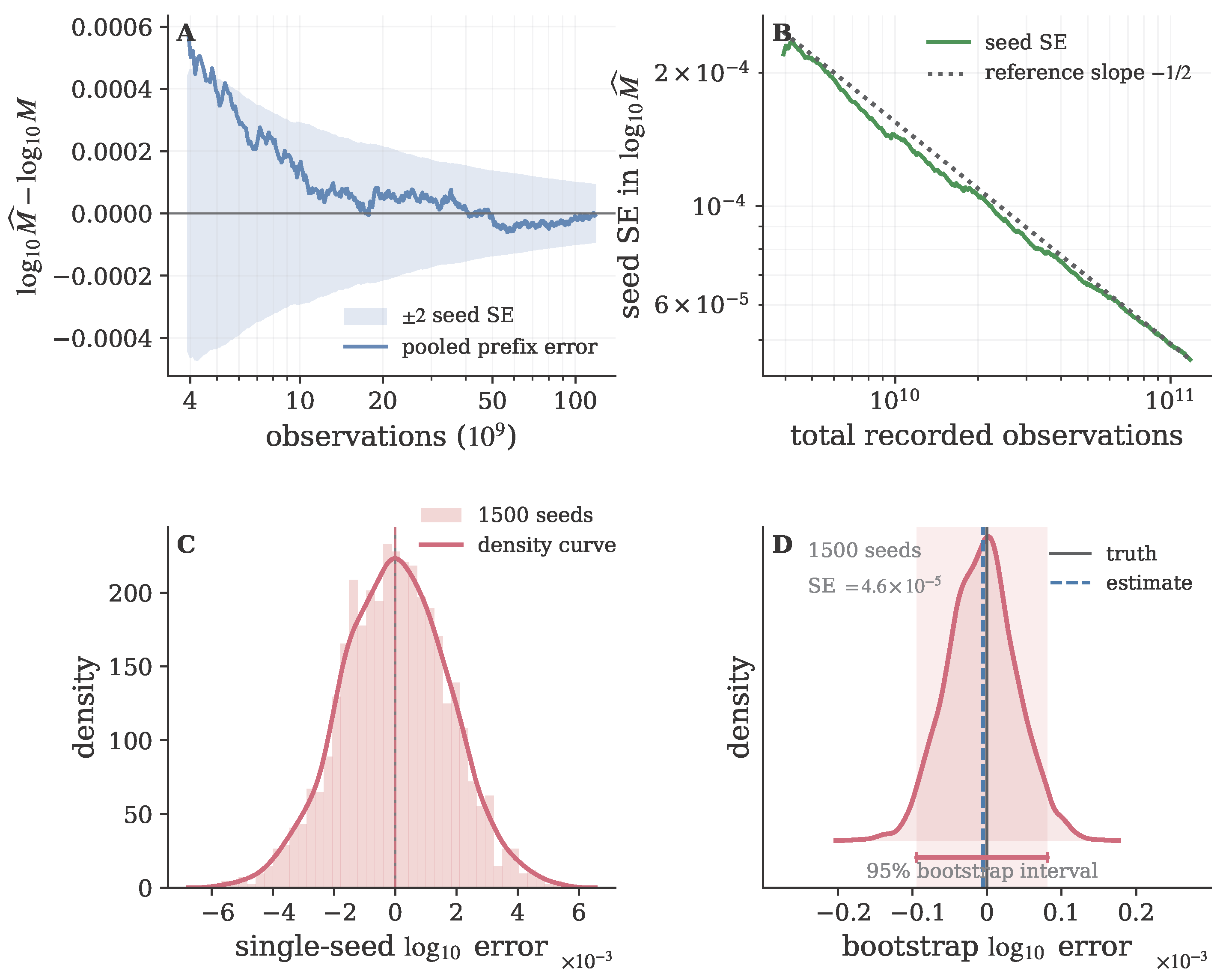
where $B_{\mathrm{tot}}=S{q}_n$ is the total number of recorded post-burn-in states in S complete seeds. The centering quantity is the expectation of the corresponding finite protocol. Figure 3 tests this behavior for the $M\left(9\right)$ production run by pooling increasing seed prefixes and recomputing the full reconstruction.

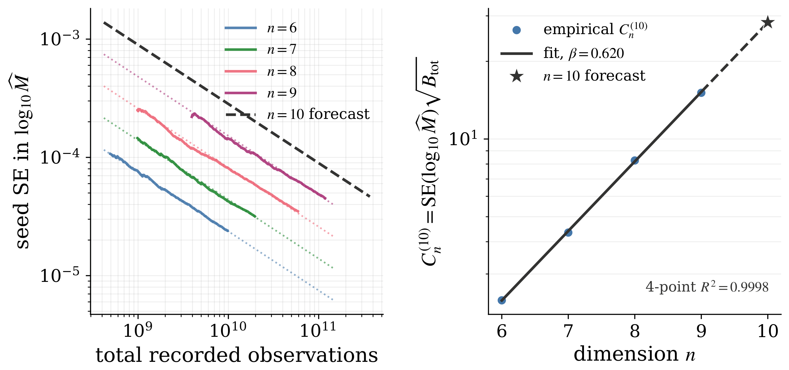
The cross-n experiment estimates the dimensional growth of $C_{n,\mathrm{prot}}^{\left(10\right)}$. For $n=6,7,8,9$, we fit

$$\log \mathrm{SE}({\log }_{10}\widehat{M}\left(n\right);B_{\mathrm{tot}})=\alpha +\beta n-{\displaystyle \frac{1}{2}}\log B_{\mathrm{tot}}+{\epsilon }_{n,B},$$

with the exponent fixed at the Monte Carlo value $-1/2$. The fitted values are

$$\beta =0.620093,\exp \left(\beta \right)=1.8591,\exp \left(2\beta \right)=3.4563.$$

Thus, at a fixed budget, the seed-level ${\log }_{10}$ standard error increases by a factor of about $1.86$ per added dimension, whereas maintaining a fixed standard error requires about $3.46$ times as many recorded states per added dimension. The fitted seed-replication constant in ${\log }_{10}$ units for $n=10$ is $C_{10,\mathrm{prot}}^{\left(10\right)}=28.2991$, so an $M\left(10\right)$ run with total recorded budget $B_{\mathrm{tot}}$ has the seed-level forecast

$$\mathrm{SE}({\overline{L}}_{10,S}/\log 10)\approx 28.2991B_{\mathrm{tot}}^{-1/2}.$$

This forecast sets the budget scale for Section 3.2; Figure 4 shows the fitted curves.

The cross-dimensional fit is based on the four dimensions $n=6,7,8,9$, with the budget exponent $-1/2$ fixed in advance. The iid seed-replication CLT supports the $B_{\mathrm{tot}}^{-1/2}$ dependence for each fixed dimension. The variation in the prefactor with n is estimated empirically from these runs, and the value at $n=10$ is an extrapolative budget forecast. Cross-dimensional extrapolation uncertainty is reported separately from the seed-level standard error. The forecast sets the production budget and provides an empirical variability scale.

The high-precision known-value runs give the finite-n benchmark points in

Table 2. High-precision known-value backtests. Chains/layer is the actual number of Markov chains run on each sampled layer. Errors and standard errors are in ${\log }_{10}$ scale.

n	Seeds	Chains/Layer	${\log }_{10}\widehat{\mathit{M}}\left(\mathit{n}\right)$	${\log }_{10}$ Err.	${\log }_{10}$ SE	z
8	3000	2048	$22.749197804918$	$-6.2026\times {10}^{-7}$	$3.5028\times {10}^{-5}$	$-0.02$
9	1500	4096	$41.456947495132$	$-5.1645\times {10}^{-6}$	$4.5119\times {10}^{-5}$	$-0.11$

. Their ${\log }_{10}$ errors lie within the independently estimated seed-level variability. The full Monte Carlo parameters are collected in

Table A1. Monte Carlo parameter summary for the numerical experiments. Here, c is the actual number of Markov chains run on each sampled layer, and m is the number of recorded states per chain.

Experiment	Layers	c	m	Burn-In	Thin.	Seeds
$M\left(8\right)$ high precision/convergence	$n=8$, duality, 128 sampled	2048	75	2500	40	3000
$M\left(9\right)$ high precision	$n=9$, duality, 256 sampled	4096	75	2500	40	1500
$M\left(10\right)$ production estimate	$n=10$, duality, 512 sampled	8192	75	2500	40	1000
Cross-n scaling	$n=6,7,8,9$, duality	see note	75	2500	40	$1000,1000,3000,1500$
Truth-free closure	$n=8$, all nontrivial layers	256	75	2500	40	20
Burn-in/thinning drift	$n=8$, duality, 128 sampled	256	75	$2500,5000,10000$	$40,80,120$	$40,40,40$
Chain-layout invariance	$n=8$, duality, 128 sampled	see note	see note	2500	40	20 per layout

For the cross-n scaling experiment, the chains per sampled layer for $n=6,7,8,9$ are $4096,4096,2048,$ and 4096, respectively; the budget variable is equal to the total recorded observations obtained by adding independent seeds. The chain-layout rows use three equal-budget layouts: $256\times 75$, $64\times 300$, and $16\times 1200$ chains by recorded states per chain.

. For context, direct finite-n substitution of published asymptotic formulae is reported in

Table A2. Direct finite-n substitution of published asymptotic formulae, with the corresponding ${\log }_{10}$ errors from this work where a high-precision known-value backtest is reported. Errors are relative to the exact $M\left(n\right)$. The $j\le 2$ row is the Korshunov–Sapozhenko approximation, equivalently the first two cluster-expansion terms in the normalization of [27].

n	Formula	Exact	Asymp.	Asymp. Err.	This Work	This Work Err.
		${\mathbf{log}}_{\mathbf{10}}\mathit{M}\left(\mathit{n}\right)$	${\mathbf{log}}_{\mathbf{10}}\tilde{\mathit{M}}\left(\mathit{n}\right)$	${\mathbf{log}}_{\mathbf{10}}(\tilde{\mathit{M}}/\mathit{M})$	${\mathbf{log}}_{\mathbf{10}}\widehat{\mathit{M}}\left(\mathit{n}\right)$	${\mathbf{log}}_{\mathbf{10}}(\widehat{\mathit{M}}/\mathit{M})$
7	KS / CE $j\le 2$	$12.382859952093$	$12.363048150434$	$-1.9812\times {10}^{-2}$	–	–
7	CE $j\le 3$		$12.488696845908$	$1.0584\times {10}^{-1}$
7	CE $j\le 4$		$12.576910945211$	$1.9405\times {10}^{-1}$
8	KS / CE $j\le 2$	$22.749198425175$	$22.687132301056$	$-6.2066\times {10}^{-2}$	$22.749197804918$	$-6.2026\times {10}^{-7}$
8	CE $j\le 3$		$22.717315202061$	$-3.1883\times {10}^{-2}$
8	CE $j\le 4$		$22.731045948010$	$-1.8152\times {10}^{-2}$
9	KS / CE $j\le 2$	$41.456952659651$	$40.947270539746$	$-5.0968\times {10}^{-1}$	$41.456947495132$	$-5.1645\times {10}^{-6}$
9	CE $j\le 3$		$41.115843278861$	$-3.4111\times {10}^{-1}$
9	CE $j\le 4$		$41.228984400789$	$-2.2797\times {10}^{-1}$

Blank entries repeat the exact value or the present-work estimate shown on the first row for the same n.

.

3.2. Protocol Estimate for $M\left(10\right)$

The same estimator under the stated protocol can be applied to $M\left(10\right)$, where no exact value is available. The known cases $n\le 9$ calibrate the budget scale through the cross-n scaling experiment; Appendix A.1 records the layer set, chain layout, burn-in, thinning, and reconstruction rule. The resulting protocol estimate is reported in

Table 3. $M\left(10\right)$ protocolestimate and variability summary.

Quantity	Value	Notes
Total recorded states	$\mathrm{314,572,800,000}$	production run total
Number of seeds	1000	independent production seeds
${\log }_{10}\widehat{M}\left(10\right)$	$78.951142528342$	primary estimate
$\widehat{M}\left(10\right)$	$8.9360\times {10}^{78}$	value-scale rendering
Seed SE for ${\log }_{10}\widehat{M}\left(10\right)$	$5.3089\times {10}^{-5}$	seed-level variability
Bootstrap interval	$78.951143\pm 1.04\times {10}^{-4}$	$95\%$${\log }_{10}$-scale interval
Jackknife SE	$5.3089\times {10}^{-5}$	stability check
Split-half difference	$6.7109\times {10}^{-5}$	absolute ${\log }_{10}$-scale difference
Cross-n budget forecast	$78.951143\pm 5.0456\times {10}^{-5}$	forecast from the fitted scaling law

.

The seed and jackknife standard errors and the bootstrap interval in Table 3 quantify uncertainty arising from repeat-to-repeat variability under the fixed protocol; they do not account for systematic effects shared across seeds. The bootstrap half-width $1.04\times {10}^{-4}$ on the ${\log }_{10}$ scale corresponds to a multiplicative half-width of about $2.4\times {10}^{-4}$. Separately, applying the fitted cross-n seed-replication scaling law $\mathrm{SE}({\overline{L}}_{10,S}/\log 10)\approx 28.2991B_{\mathrm{tot}}^{-1/2}$ to the reported production budget gives $\mathrm{SE}({\overline{L}}_{10,S}/\log 10)\approx 5.0456\times {10}^{-5}$. As a computational scale reference, a 1000-seed run at about 30 min per seed on one RTX 5080 corresponds to roughly 500 RTX 5080 GPU-hours. The cross-n quantity is an extrapolative budget forecast based on lower-dimensional runs.

3.3. Whitney-Number Shape

The estimator reconstructs the Whitney numbers, not only the total sum $M\left(n\right)$. Here,

$$a_n\left(k\right)=\#\{D\subseteq B_n:D\mathrm{is}\mathrm{a}\mathrm{downset}\mathrm{and}|D|=k\}$$

is the k-th Whitney number of the ideal lattice $\mathcal{I}\left(B_n\right)$, ranked by ideal cardinality. With the two endpoint ideals omitted, the same rows appear in OEIS A269699 and are described there as empirically unimodal [19]. The shape of this Whitney-number sequence is also connected to open Sperner-theoretic questions for $\mathcal{I}\left(B_n\right)$, including unimodality, the rank-unimodal and strongly Sperner (RUSS) property, Peck-type consequences, and symmetric chain decompositions [44,45,46,47].

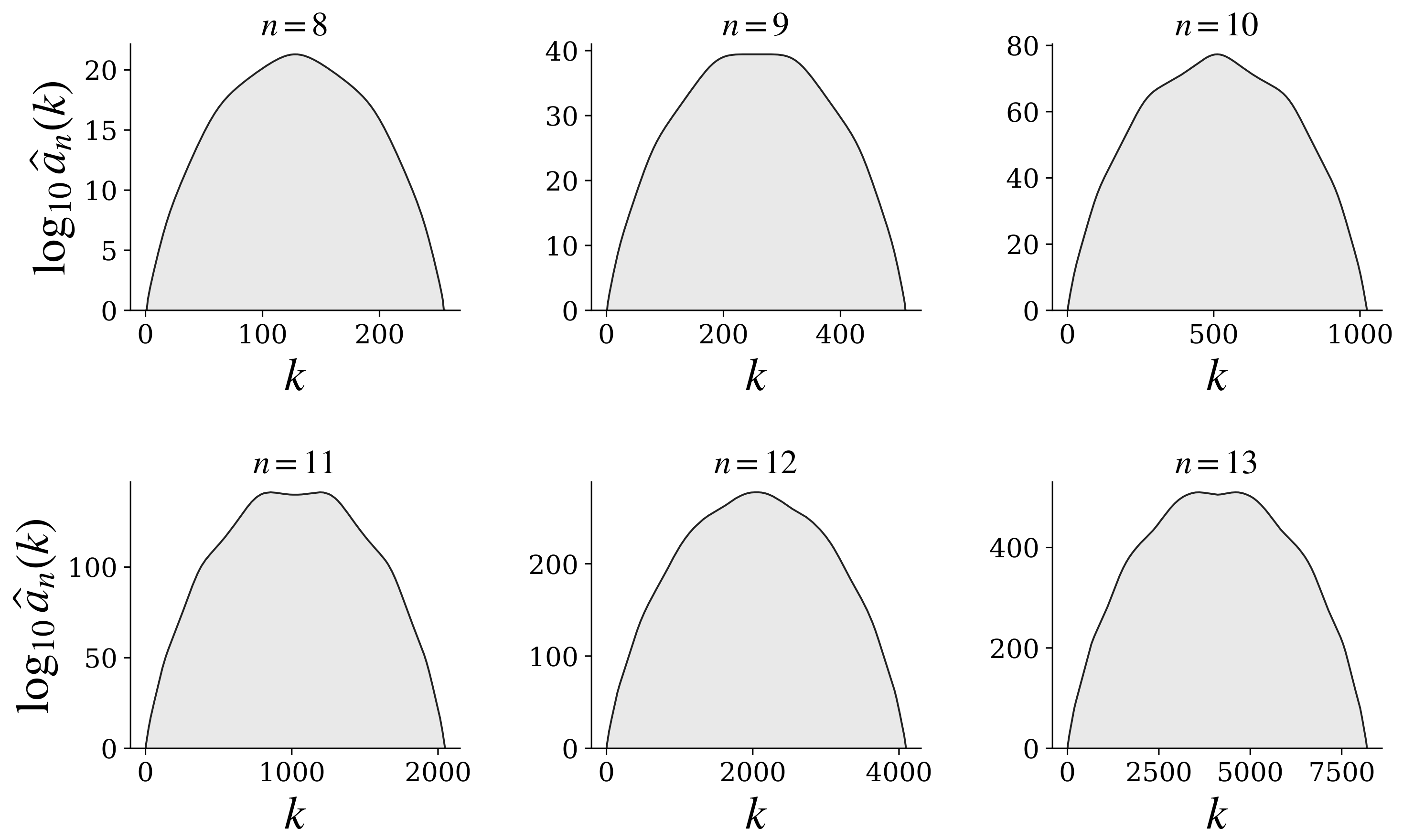
Figure 5 shows the estimated Whitney-number sequences for $n=8,\dots ,13$. The odd cases display a center valley between two symmetric shoulders.

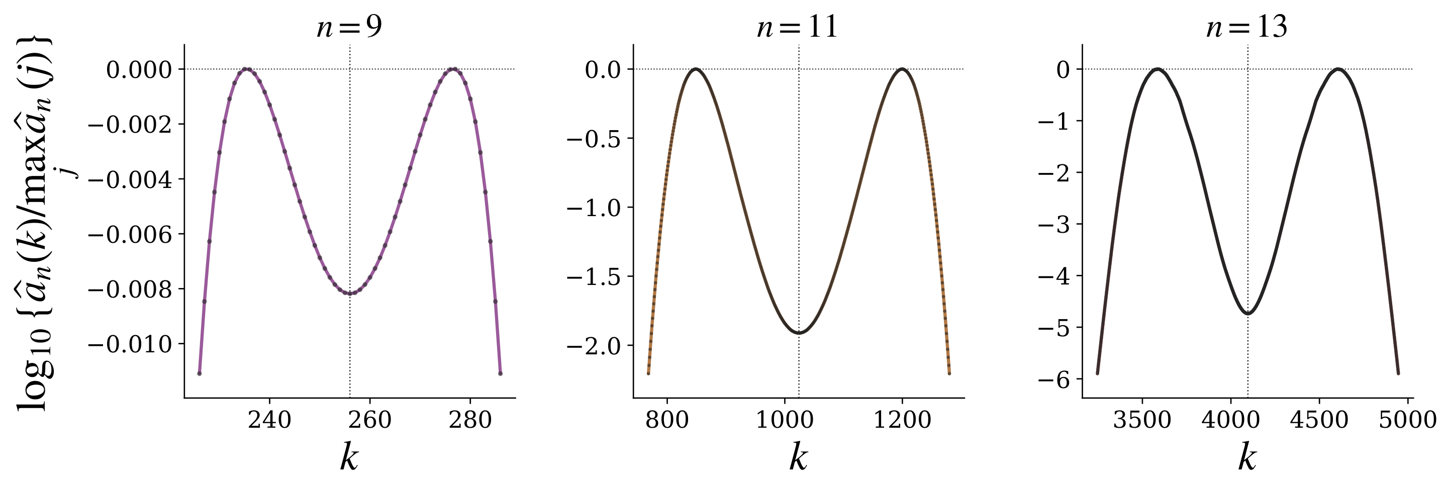
For $n=9$, the feature is small but numerically separated in the seed-level contrast analysis. The estimated Whitney-number sequence has symmetric shoulders at $k=235$ and $k=277$. The independent sampled contrast is

$${\log }_{10}{\widehat{a}}_9\left(235\right)-{\log }_{10}{\widehat{a}}_9\left(256\right)=0.008184090729,$$

with seed SE $9.31\times {10}^{-6}$, bootstrap 95% interval $[0.008166,0.008202]$, and shoulder-to-center ratio $1.019023$. The same high-precision run has ${\log }_{10}$ error $-5.1645\times {10}^{-6}$ for $M\left(9\right)$. The estimated $n=9$ profile therefore has two symmetric shoulders above the center and differs from the empirical unimodality description in OEIS A269699. An independent study by Alex Fihman, Lennart Van Hirtum, and Christian Plessl [48] combined a weight-layer branching estimator with pair matching and a degree-corrected MCMC procedure. Its comparison of MBF₉ MCMC samples with uniformly sampled reference data shows a bimodal weight distribution associated with the two middle Boolean layers. This result provides independent empirical support for the two-shoulder feature observed in our reconstructed profile.

The $n=11$ and $n=13$ panels in Figure 6 show the same picture in the plotted windows. The shoulder-to-center ratios in the estimated windows are approximately $81.6$ for $n=11$ and $5.46\times {10}^4$ for $n=13$.

4. Discussion

The method provides a finite-n Monte Carlo reconstruction that complements exact enumeration. It recovers the Whitney-number profile from local adjacent-layer ratios and sums that profile to estimate $M\left(n\right)$. Asymptotic and cluster-expansion formulae remain important reference points for the scale of $M\left(n\right)$, but they do not by themselves provide a data-driven uncertainty estimate for a specific unknown finite case.

Although the reconstruction is a product of adjacent ratios on the original scale, the calculation is carried out in log space. Local ratio errors therefore accumulate additively in the reconstructed log Whitney numbers. To the first order,

$$\mathrm{Var}\left(\log \widehat{M}\left(n\right)\right)\approx s^{\top }\mathsf{\Sigma }s,$$

where s is the sensitivity of the log-sum-exp reconstruction to the adjacent log-ratios and $\mathsf{\Sigma }$ is their Monte Carlo covariance. The known-value tests and cross-n scaling measure this accumulated error after reconstruction.

The two-shoulder structure in odd-dimensional cases is a counterintuitive feature of the reconstructed Whitney-number profile. The rank-unimodality of this sequence is an empirical description in this setting, not a consequence of the exact rank duality. The duality $a_n\left(k\right)=a_n(2^n-k)$ only enforces symmetry of the profile about the center. It does not require the central coefficient $a_n\left(2^{n-1}\right)$ to be maximal. Therefore, a symmetric two-shoulder profile, with a center valley between two equal off-center shoulders, is compatible with the duality even though it contradicts unimodality. A mathematical explanation of this structure remains open; the evidence presented here is numerical and restricted to a finite n.

The long-chain law of Proposition 2 applies when the number of post-burn-in records per chain tends to infinity. The cross-dimensional experiment instead repeats a fixed finite protocol and estimates the seed-replication coefficient

$$\mathrm{SE}\left({\overline{L}}_{n,S}\right)=C_{n,\mathrm{prot}}{B}_{\mathrm{tot}}^{-1/2}$$

around that protocol’s expectation. The cross-n fit estimates how $C_{n,\mathrm{prot}}$ changes with dimension. In the tested dimensions, this change appears regular: at a fixed recorded-state budget, the seed-level log standard error grows by about a factor $1.86$ per added dimension. We use this empirical regularity as a budget forecast for $C_{n,\mathrm{prot}}$. One possible explanation is that the final log-sum-exp is most sensitive to the part of the reconstructed Whitney-number profile carrying the largest mass, so the effective error propagation may be governed by a relatively narrow central range of adjacent ratios. If the local addable/removable statistics and chain autocorrelations in that range change regularly with n, then the fitted prefactor $C_n$ can also vary regularly. This explanation is heuristic.

The known-value backtests at $M\left(8\right)$ and $M\left(9\right)$ are consistent with the measured seed-level variability, and the cross-n experiment gives a practical budget scale for $M\left(10\right)$. The principal limitation is that the combinatorial identity determines the exact target ratios but does not guarantee the finite-run accuracy of their Monte Carlo estimates. Finite-run mixing, autocorrelation, and error propagation through the reconstructed log Whitney numbers therefore remain empirical diagnostics.

5. Conclusions

This work reformulates Dedekind-number estimation as the reconstruction of the Whitney numbers of $\mathcal{I}\left(B_n\right)$ across fixed-cardinality downset layers. Rather than sampling the total set of monotone Boolean functions directly, the method estimates local averages of the numbers of addable and removable elements on each layer. The adjacent-layer double-counting identity converts these averages into the ratios $a_n(k+1)/a_n\left(k\right)$, and log-space accumulation together with Boolean-lattice duality gives the full reconstructed profile ${\left({\widehat{a}}_n\left(k\right)\right)}_{k=0}^{2^n}$. The Dedekind-number estimate $\widehat{M}\left(n\right)$ is then obtained by summing this profile.

Under the fixed protocol, the $n=8$ and $n=9$ estimates agree with the known Dedekind numbers within the measured seed-level variability and exhibit the expected Monte Carlo scaling. For $n=10$, the same protocol gives

$$\widehat{M}\left(10\right)=(8.9360\pm 0.0010)\times {10}^{78},$$

where the displayed uncertainty is the value-scale expression of the cross-n budget forecast. The reconstruction also supplies rank-shape information. For $n=9$, the Whitney-number profile has two symmetric shoulders above the center, contrary to the empirical unimodality description in OEIS A269699. The $n=11$ and $n=13$ center-window estimates show the same center-valley pattern with higher contrast.

References

1. Dedekind, R. Über zerlegungen von zahlen durch ihre grössten gemeinsamen theiler. In Fest-Schrift der Herzoglichen Technischen Hochschule Carolo-Wilhelmina; Vieweg+Teubner Verlag: Wiesbaden, Germany, 1897; pp. 1–40. [Google Scholar] [CrossRef] [Scilit]
2. Church, R. Numerical analysis of certain free distributive structures. Duke Math. J. 1940, 6, 732–734. [Google Scholar] [CrossRef] [Scilit]
3. Ward, M. Note on the order of the free distributive lattice. Bull. Am. Math. Soc. 1946, 52, 423. [Google Scholar] [CrossRef] [Scilit]
4. Yamamoto, K. Logarithmic order of free distributive lattice. J. Math. Soc. Jpn. 1954, 6, 343–353. [Google Scholar] [CrossRef] [Scilit]
5. Wiedemann, D. A computation of the eighth Dedekind number. Order 1991, 8, 5–6. [Google Scholar] [CrossRef] [Scilit]
6. Fidytek, R.; Mostowski, A.W.; Somla, R.; Szepietowski, A. Algorithms counting monotone Boolean functions. Inf. Process. Lett. 2001, 79, 203–209. [Google Scholar] [CrossRef] [Scilit]
7. De Causmaecker, P.; De Wannemacker, S. On the number of antichains of sets in a finite universe. arXiv 2014, arXiv:1407.4288. [Google Scholar]
8. Berman, J.; Köhler, P. On Dedekind numbers and two sequences of Knuth. J. Integer Seq. 2021, 24, 3. [Google Scholar]
9. A Campo, F. A flexible approach for the enumeration of down-sets and its application on Dedekind numbers. arXiv 2022, arXiv:2206.10293. [Google Scholar]
10. Stephen, T.; Yusun, T. Counting inequivalent monotone Boolean functions. Discret. Appl. Math. 2014, 167, 15–24. [Google Scholar] [CrossRef] [Scilit]
11. Pawelski, B. On the number of inequivalent monotone Boolean functions of 8 variables. J. Integer Seq. 2022, 25, 22.7.7. [Google Scholar]
12. Szepietowski, A. Fixes of permutations acting on monotone Boolean functions. J. Integer Seq. 2022, 25, 22.9.6. [Google Scholar]
13. Pawelski, B. On the number of inequivalent monotone Boolean functions of 9 variables. IEEE Trans. Inf. Theory 2024, 70, 5358–5364. [Google Scholar] [CrossRef] [Scilit]
14. Jäkel, C. A computation of the ninth Dedekind number. J. Comput. Algebra 2023, 6–7, 100006. [Google Scholar] [CrossRef] [Scilit]
15. Van Hirtum, L.; De Causmaecker, P.; Goemaere, J.; Kenter, T.; Riebler, H.; Lass, M.; Plessl, C. A computation of the ninth Dedekind number using FPGA supercomputing. ACM Trans. Reconfig. Technol. Syst. 2024, 17, 1–28. [Google Scholar] [CrossRef] [Scilit]
16. De Causmaecker, P.; Van Hirtum, L. Solving systems of equations on antichains for the computation of the ninth Dedekind number. J. Comb. Optim. 2026, 51, 5. [Google Scholar] [CrossRef] [Scilit]
17. Pawelski, B.; Szepietowski, A. Divisibility properties of Dedekind numbers. J. Integer Seq. 2023, 26, 23.7.7. [Google Scholar]
18. Stanley, R.P. Enumerative Combinatorics; Volume 1, The Wadsworth & Brooks/Cole Mathematics Series; Wadsworth & Brooks/Cole: Monterey, CA, USA, 1986. [Google Scholar] [CrossRef] [Scilit]
19. Rorabaugh, D. A269699: Irregular Triangle Read by Rows: Number of k-Element Proper Ideals of the n-Dimensional Boolean Lattice. 2016. Available online: https://oeis.org/A269699 (accessed on 3 September 2026).
20. Kleitman, D.J. On Dedekind’s problem: The number of monotone Boolean functions. Proc. Am. Math. Soc. 1969, 21, 677–682. [Google Scholar] [CrossRef] [Scilit]
21. Kleitman, D.J.; Markowsky, G. On Dedekind’s problem: The number of isotone Boolean functions. II. Trans. Am. Math. Soc. 1975, 213, 373–390. [Google Scholar] [CrossRef] [Scilit]
22. Korshunov, A.D. Solution of Dedekind’s problem on the number of monotonic Boolean functions. Dokl. Akad. Nauk SSSR 1977, 233, 543–546. [Google Scholar]
23. Korshunov, A.D. Monotone Boolean functions. Russ. Math. Surv. 2003, 58, 929–1001. [Google Scholar] [CrossRef] [Scilit]
24. Kahn, J. Entropy, independent sets and antichains: A new approach to Dedekind’s problem. Proc. Am. Math. Soc. 2002, 130, 371–378. [Google Scholar] [CrossRef] [Scilit]
25. Ilinca, L.; Kahn, J. Counting maximal antichains and independent sets. Order 2013, 30, 427–435. [Google Scholar] [CrossRef] [Scilit]
26. Korshunov, A.D.; Shmulevich, I. On the distribution of the number of monotone Boolean functions relative to the number of lower units. Discret. Math. 2002, 257, 463–479. [Google Scholar] [CrossRef] [Scilit]
27. Jenssen, M.; Malekshahian, A.; Park, J. On Dedekind’s problem, a sparse version of Sperner’s theorem, and antichains of a given size in the Boolean lattice. arXiv 2024, arXiv:2411.03400. [Google Scholar]
28. Biswas, A.; Sarkar, P. Counting unate and monotone Boolean functions under restrictions of balancedness and non-degeneracy. J. Integer Seq. 2025, 28, 25.3.4. [Google Scholar]
29. Pawelski, B.; Szepietowski, A. Counting self-dual monotone Boolean functions. J. Integer Seq. 2025, 28, 25.6.5. [Google Scholar]
30. Park, J.; Sarantis, M.; Tetali, P. Note on the number of antichains in generalizations of the Boolean lattice. Comb. Theory 2025, 5, 7. [Google Scholar] [CrossRef] [Scilit]
31. Falgas-Ravry, V.; Räty, E.; Tomon, I. Dedekind’s problem in the hypergrid. Adv. Math. 2026, 488, 110796. [Google Scholar] [CrossRef] [Scilit]
32. Jenssen, M.; Park, J.; Sarantis, M. On the number of antichains in {0,1,2}n. arXiv 2026, arXiv:2601.07650. [Google Scholar]
33. De Oliveira, P.M.C.; Penna, T.J.P.; Herrmann, H.J. Broad histogram method. Braz. J. Phys. 1996, 26, 677–683. [Google Scholar] [CrossRef] [Scilit]
34. De Oliveira, P.M.C. Broad histogram relation is exact. Eur. Phys. J. B 1998, 6, 111–115. [Google Scholar] [CrossRef] [Scilit]
35. Chatterjee, S.; Diaconis, P.; Holmes, S. Estimating the size of a set using cascading exclusion. arXiv 2025, arXiv:2508.05901. [Google Scholar]
36. MacMahon, P.A. Memoir on the theory of the partitions of numbers. Part II. Proc. R. Soc. Lond. 1899, 64, 224–227. [Google Scholar] [CrossRef] [Scilit]
37. MacMahon, P.A., IX. Memoir on the theory of the partitions of numbers. Part VI. Partitions in two-dimensional space, to which is added an adumbration of the theory of the partitions in three-dimensional space. Philos. Trans. R. Soc. Lond. Ser. A 1912, 211, 345–373. [Google Scholar] [CrossRef] [Scilit]
38. Xiang, S.; Feng, H.; Zhuo, K.; Chen, T.S.; Zhang, K. Charge functions for odd dimensional partitions. J. High Energy Phys. 2026, 2026, 141. [Google Scholar] [CrossRef] [Scilit]
39. Metropolis, N.; Rosenbluth, A.W.; Rosenbluth, M.N.; Teller, A.H.; Teller, E. Equation of state calculations by fast computing machines. J. Chem. Phys. 1953, 21, 1087–1092. [Google Scholar] [CrossRef] [Scilit]
40. Hastings, W.K. Monte Carlo sampling methods using Markov chains and their applications. Biometrika 1970, 57, 97–109. [Google Scholar] [CrossRef]
41. Levin, D.A.; Peres, Y.; Wilmer, E.L. Markov Chains and Mixing Times; American Mathematical Society: Providence, RI, USA, 2009. [Google Scholar] [CrossRef] [Scilit]
42. Markowsky, G. The level polynomials of the free distributive lattices. Discret. Math. 1980, 29, 275–285. [Google Scholar] [CrossRef] [Scilit]
43. Efron, B.; Tibshirani, R.J. An Introduction to the Bootstrap; Chapman & Hall/CRC: New York, NY, USA, 1993. [Google Scholar] [CrossRef] [Scilit]
44. McHard, R.W. Sperner Properties of the Ideals of a Boolean Lattice. Ph.D. Thesis, University of California, Riverside, CA, USA, 2009. [Google Scholar]
45. Engel, K. Sperner Theory; Cambridge University Press: Cambridge, UK, 1997. [Google Scholar] [CrossRef] [Scilit]
46. Greene, C.; Kleitman, D.J. Strong versions of Sperner’s theorem. J. Comb. Theory Ser. A 1976, 20, 80–88. [Google Scholar] [CrossRef] [Scilit]
47. Proctor, R.A.; Saks, M.E.; Sturtevant, D.G. Product partial orders with the Sperner property. Discret. Math. 1980, 30, 173–180. [Google Scholar] [CrossRef] [Scilit]
48. Fihman, A.; Van Hirtum, L.; Plessl, C. Statistical estimation of higher Dedekind numbers. arXiv 2026, arXiv:2607.08446. [Google Scholar]
Figure 1. Boxed-partition view of the first Boolean boxes. Colored boxes form a downset: if a box is occupied, every coordinatewise smaller box is occupied. Within each dimension, configurations are grouped by their number k of occupied boxes, i.e., by the cardinality layer Ω n , k . The Whitney numbers shown in each row sum to M ( 1 ) = 3 , M ( 2 ) = 6 , and M ( 3 ) = 20 . Green arrows indicate adjacent-layer moves that add one box; red arrows indicate the reverse moves that remove one box.
Mathematics 14 03300 g001
Figure 2. Three-dimensional B 3 schematic of the fixed-layer sampling mechanism. Solid green arrows inside Ω n , k represent exchange moves of the Markov chain within the fixed-cardinality layer; the miniature states are valid B 3 downsets drawn for visualization. Dashed orange arrows to Ω n , k 1 and dashed blue arrows to Ω n , k + 1 represent boundary measurements of removable and addable choices used to estimate E k R and E k A , not transitions of a global chain. Adjacent layer ratios are then reconstructed from the exact adjacent-layer identity.
Mathematics 14 03300 g002
Figure 3. M ( 9 ) convergence under seed-prefix pooling for the fixed production protocol. Panel (A) shows the pooled prefix log 10 error, with shading indicating a ± 2 seed-standard-error band. Panel (B) shows the corresponding seed standard error in log 10 units; the dotted line indicates the Monte Carlo reference slope 1 / 2 . Panel (C) shows the histogram of the 1500 single-seed log 10 errors and its overlaid density curve; the vertical dashed line marks zero error. Panel (D) shows the seed-bootstrap distribution of the final 1500-seed estimator. The solid black and dashed blue vertical lines mark the true value and the estimate, respectively, and the shaded interval indicates the 95% bootstrap interval.
Mathematics 14 03300 g003
Figure 4. Cross-n scaling of the seed-level log 10 variability for n = 6 , 7 , 8 , 9 , together with the fitted n = 10 forecast. The dashed lines show the fitted scaling curves, including the n = 10 forecast. The fit constrains the budget exponent to the Monte Carlo value 1 / 2 and estimates the remaining growth with n.
Mathematics 14 03300 g004
Figure 5. EstimatedWhitney-number sequences for n = 8 , , 13 , displayed as log 10 a ^ n ( k ) . The n = 8 and n = 9 panels are high-precision backtest estimates, n = 10 is the protocol estimate, and n = 11 , 12 , 13 are center-window estimates.
Mathematics 14 03300 g005
Figure 6. Center zooms for the odd cases n = 9 , 11 , 13 , displayed as log 10 { a ^ n ( k ) / max j a ^ n ( j ) } within each plotted window. The vertical dashed lines mark the central rank k = 2 n 1 . The n = 9 panel comes from the high-precision estimate and shows a shallow but resolved double shoulder: the sampled shoulder occurs at k = 235 , its dual is k = 277 , and the shoulder-to-center ratio is about 1.019 . The n = 11 and n = 13 panels are center-window estimates and show an analogous center-valley pattern with higher contrast.
Mathematics 14 03300 g006