FrontierStep-RL: Fixed-Dimensional Structured Actions for Transaction-Cost-Aware Portfolio Reinforcement Learning

Abstract

Portfolio reinforcement learning (RL) commonly represents each action as a complete asset-weight vector, causing the action dimension and exploration difficulty to grow with the investment universe. This study proposes FrontierStep-RL, which replaces the direct N-dimensional action with two bounded variables: a frontier coordinate and a rebalancing step. At each decision date, rolling estimates of expected returns and covariance define a regularized efficient frontier. A cost–risk-aware coordinate organizes the frontier using normalized local changes in predicted volatility and one-way turnover. The coordinate selects a frontier-supported target portfolio, while the step controls how far the pre-trade portfolio moves toward that target. We evaluate FrontierStep-RL on FF49, FF100, and FNSPID-50 against traditional strategies, controlled direct-weight RL policies, and recent portfolio-management methods. FrontierStep-RL achieves net Sharpe ratios of 0.75 on both FF49 and FNSPID-50 while maintaining comparatively low volatility, drawdown, and turnover. In the 100-asset setting, it achieves 0.68, compared with 0.52 for the strongest direct-weight baseline, and completes all runs. At a transaction cost of 50 basis points, it retains net Sharpe ratios of 0.559 and 0.568. The results support fixed-dimensional target selection and controlled execution for scalable, transaction-cost-aware portfolio RL.

1. Introduction

Portfolio optimization determines how capital is allocated across financial assets under competing objectives related to return, risk, and implementation cost. The mean–variance framework of Markowitz provides the classical mathematical foundation for this problem by expressing portfolio choice through expected returns, asset covariances, and investment constraints [1]. The associated efficient frontier organizes feasible portfolios according to their estimated risk–return characteristics and remains a central reference for both theoretical analysis and practical allocation. In an investment process, however, the selected portfolio evolves after implementation. Price movements alter the relative asset weights, new observations change return and risk estimates, and the desired allocation may vary across decision dates. Portfolio management, therefore, involves a sequence of transitions from current holdings to updated targets. Dynamic trading models show that the quality of these transitions depends on the balance between the attractiveness of a new target and the cost of adjusting the existing portfolio [2].

Classical allocation methods provide structured solutions for selecting target portfolios. Global Minimum Variance reduces reliance on expected-return estimates, Risk Parity distributes risk contributions across assets, and robust mean–variance formulations account for uncertainty in the estimated inputs. Their realized performance nevertheless depends on return and covariance estimates obtained from finite and noisy historical observations. Estimation errors can generate unstable or concentrated allocations, especially when the number of assets is large relative to the available sample [3,4]. Robust sample-based procedures improve allocation stability under parameter uncertainty [5]. Regularization, practical constraint design, and transaction-cost-aware objectives further improve the implementation quality of optimized portfolios [6,7]. Robust portfolio frameworks also provide systematic guidance for uncertainty modeling and risk control [8]. Multi-period optimization extends the target-allocation problem by jointly planning expected return, risk, transaction costs, and future trades over a rolling horizon [9].

Machine learning broadens the information available to portfolio models by learning nonlinear relations from high-dimensional financial data. Empirical asset-pricing studies show that nonlinear models can extract predictive information from broad collections of firm and market characteristics [10]. Machine learning has consequently been applied to expected-return estimation, risk modeling, asset ranking, and constrained portfolio construction [11]. Neural feedback strategies further connect observed market variables to adaptive allocation rules, allowing portfolio decisions to respond directly to changing financial conditions [12]. Spatial–temporal transfer-learning models in video analysis provide a related example of learning sequential representations from heterogeneous motion and appearance cues [13]. Multiview feature-fusion systems likewise combine complementary observations before joint recognition and spatial localization [14]. These developments improve the estimation and representation of investment opportunities. The financial outcome, however, is determined by the complete decision process through which a learned signal is converted into positions, risk exposure, turnover, and transaction costs.

Reinforcement learning provides a direct framework for optimizing this sequential decision process. An agent observes a financial state, selects a portfolio action, receives a reward from subsequent portfolio performance, and updates its policy through repeated interaction. Existing surveys organize portfolio RL research according to state representations, action spaces, reward functions, and learning algorithms [15]. Actor–critic methods have been evaluated in dynamic portfolio-selection settings using sequential investment outcomes as the learning signal [16,17]. Research on state construction incorporates heterogeneous financial information, historical risk variables, and adaptive market embeddings [18,19]. Dynamic representations further allow the policy state to respond to changing market conditions [20].

Recent portfolio RL systems address additional parts of the decision process. FreQuant represents market information across multiple frequency scales [21]. EarnMore supports customizable investment universes through maskable stock representations [22]. DeepAries jointly determines portfolio allocations and rebalancing intervals [23]. Other studies extend the objective and evaluation protocol through responsible investment criteria and comparisons with established portfolio rules [24,25]. These directions improve market representation, asset-universe flexibility, decision timing, and evaluation coverage. The representation of the portfolio action remains a central design choice because it determines how the learned state is converted into an executable allocation.

A common portfolio RL design directly generates the complete asset-weight vector from market observations [16,26]. For an investment universe containing N assets, the policy consequently operates through N asset-level outputs. The learning problem, therefore, changes with the size of the investment universe. The policy must coordinate a larger number of outputs as more assets are included, while the resulting portfolio must still satisfy full-investment, long-only, and asset-level exposure constraints. The same action vector also determines several economically distinct quantities: the cross-sectional allocation, the desired risk–return position, and the distance from the current holdings. The amount of trading required for implementation is determined only after the new weights are compared with the pre-trade portfolio.

The geometry of a direct-weight action is primarily defined by differences among portfolio weights. Weight-space proximity does not necessarily correspond to similarity in portfolio risk or transaction-cost exposure. Two nearby allocations can produce different changes in predicted volatility, while two portfolios with visibly different weight compositions can occupy similar positions in risk–return terms. The economic effect of an action, therefore, depends on the current holdings, the covariance structure, and the region of the feasible set. As the investment universe expands, the policy learns both cross-sectional allocation and these heterogeneous effects within the same growing action space.

Common action mappings improve the feasibility of direct-weight policies. Softmax and Dirichlet parameterizations produce nonnegative, fully invested portfolios, and Dirichlet policies define stochastic allocations directly on the portfolio simplex [27]. Projection and action-space decomposition support additional portfolio constraints by mapping policy outputs into a feasible allocation set [28]. These mechanisms provide useful tools for constraint handling and exploration. Their action variables remain tied to the asset-level representation, and target selection and rebalancing intensity are encoded within the same output. A structured action representation can assign these decisions separate control variables while preserving their connection to the underlying portfolio.

This study investigates such a representation through FrontierStep-RL. The central idea is to decompose a portfolio rebalance into two decisions: selecting a financially meaningful target and determining the proportion of that target implemented from the current holdings. A regularized efficient frontier provides an ordered target space, while a frontier coordinate and a rebalancing step size control the two decisions. The coordinate is organized according to local changes in portfolio risk and trading intensity, providing an economically informed path through the available targets. This formulation keeps the policy action dimension fixed as the asset universe changes and connects the learned action to both portfolio positioning and execution.

The contributions of this study comprise two methodological contributions and one empirical contribution. First, FrontierStep-RL introduces a fixed two-dimensional action representation that separates target selection from execution intensity in portfolio reinforcement learning. Second, the method organizes regularized frontier targets through a cost–risk-aware coordinate and uses a step-based transition to control movement from current holdings toward the selected target. Third, the empirical evaluation identifies three consistent patterns under a common out-of-sample protocol: the structured action maintains low cross-run variability and completes all runs as the universe expands to 100 assets; learned partial execution reduces turnover and preserves risk-adjusted performance as transaction costs increase and the cost–risk coordinate provides a more favorable risk–turnover trade-off than simpler coordinate definitions.

The remainder of this paper is organized as follows. Section 2 reviews traditional portfolio optimization, machine-learning-based portfolio methods, and reinforcement-learning-based portfolio management, with particular attention to action-space design. Section 3 presents the FrontierStep-RL formulation and policy-learning procedure. Section 4 describes the datasets, baselines, training configuration, and evaluation protocol. Section 5 reports the main experimental results. Section 6 evaluates the coordinate and action components, analyzes learned policy behavior, relates the findings to existing empirical evidence, and discusses implications, limitations, and future research. Section 7 concludes the paper.

2. Literature Review

2.1. Traditional Portfolio Optimization

Portfolio optimization is rooted in the mean–variance framework, which formulates asset allocation through expected returns, asset covariances, and investment constraints [1]. The efficient frontier organizes feasible portfolios according to their estimated risk–return characteristics and provides the theoretical basis for Global Minimum Variance, Risk Parity, and related allocation rules. Global Minimum Variance selects the feasible portfolio with the lowest estimated variance [3], whereas Risk Parity distributes portfolio risk through balanced asset-level contributions [29].

Portfolio construction also operates within the informational constraints described by the efficient market hypothesis. Under its semi-strong form, publicly available reports, announcements, and news are rapidly reflected in security prices, limiting persistent forecasting advantages based only on such information [30]. Transaction costs further raise the threshold for realized outperformance. This perspective motivates evaluating learned allocation rules net of implementation costs and against passive and structured benchmarks. FrontierStep-RL uses return-derived market histories and the stock-price component of FNSPID. The study examines how available market information is converted into feasible portfolio targets and execution decisions.

These formulations provide interpretable target portfolios, but their realized quality depends on parameters estimated from finite and noisy return samples. Expected-return estimates are particularly sensitive to sampling variation, and covariance estimates become less stable when the number of assets is large relative to the observation window. The optimizer can, therefore, amplify small input changes into large differences in portfolio weights, producing concentrated allocations and unstable out-of-sample behavior.

Shkolnik et al. [4] examine the effect of estimation uncertainty on portfolio selection, while Petukhina et al. [5] develop robust procedures for sample-based allocation. Regularized and implementation-aware formulations further stabilize target construction. Transaction-cost-aware mean–variance optimization aligns the objective with realized net performance [6], and practical multi-asset extensions introduce covariance stabilization and allocation constraints [7].

Robust portfolio frameworks also organize uncertainty sets, risk measures, and constraint choices according to the investment setting [8]. Related studies have investigated ${\ell }_1$-regularized machine-learning formulations and robust sparse optimization models for portfolio selection under estimation uncertainty [31,32]. This research stream primarily improves the financial quality, statistical stability, and feasibility of the target portfolio.

Variance-based risk measures can be complemented by quantile-based downside-risk measures. Value-at-Risk (VaR) summarizes a loss quantile at a chosen confidence level and has been studied as a constraint on dynamic portfolio policies, while Conditional Value-at-Risk (CVaR), or expected shortfall, evaluates losses beyond the VaR threshold and supports tractable optimization formulations under standard portfolio-loss models [33,34]. These measures are particularly relevant when an investment mandate emphasizes tail-loss control rather than symmetric return dispersion. In the present framework, covariance risk is used to construct an ordered regularized target path. Future work could investigate target generators based on VaR, CVaR, or related downside-risk measures while retaining the target-selection and step-controlled execution decomposition.

A related line of work studies how an existing portfolio should move toward a time-varying target. Immediate replacement of the current allocation can generate high turnover because successive solutions respond to new observations and changing market conditions. Dynamic trading models, therefore, represent portfolio updates as partial adjustments that balance the expected benefit of the new target against the cost of changing current positions.

Gârleanu and Pedersen [2] derive state-dependent trading policies in which the updated portfolio combines current holdings with a moving target, giving the adjustment magnitude a direct economic interpretation. Boyd et al. [9] formulate single-period and multi-period trading through convex optimization that jointly considers expected return, risk, transaction costs, holding costs, and future positions.

Together, these studies address three connected problems: constructing an interpretable risk–return target, stabilizing that target under estimation uncertainty, and planning a cost-aware transition from the current portfolio. Their decisions are commonly generated by repeatedly solving an optimization problem from estimated inputs. Sequential learning provides a complementary mechanism in which market information determines both the selected target and the degree to which it is implemented.

2.2. Machine Learning-Based Portfolio Optimization

Machine learning extends portfolio analysis by extracting nonlinear relations from high-dimensional financial data. A recent review organizes quantitative portfolio management around portfolio optimization, risk parity, style integration, and machine learning, highlighting the growing interaction between financial structure and data-driven methods [35]. Gu, Kelly, and Xiu [10] show that nonlinear models can identify predictive information from broad collections of firm and market characteristics. Attention-enhanced residual generative models have also paired representation learning with chaotic particle-swarm hyperparameter optimization in image-security tasks [36].

Lee et al. [11] review applications of machine learning to expected-return estimation, risk modeling, asset ranking, and constrained portfolio construction. Machine-learning-based portfolio systems differ in how the learned information enters the allocation process. Some methods estimate returns, risks, or asset scores and pass them to a separate optimizer. Neural feedback strategies instead express portfolio decisions directly as functions of observed financial variables [12]. Hybrid neuro-fuzzy systems provide a cross-domain example in which predicted demand directly informs real-time resource allocation [37].

Deep learning expands the representation capacity of these systems. Data-fusion architectures combine heterogeneous variables into a common portfolio state [18]. Communication-aware transferable fusion extends this idea to collaborative perception under bandwidth and domain-shift constraints [38]. Historical price and risk encoders capture temporal patterns relevant to allocation [19], while deep portfolio models connect sequential market features with portfolio outcomes [39]. Dynamic embeddings allow the representation to adapt to changing market conditions [20]. Visual–inertial fusion similarly uses geometric structure to combine heterogeneous observations before state estimation [40]. Graph-convolutional wavelet models with meta-learning provide a cross-domain example of representing nonlinear, multi-scale, time-varying dynamics in coupled systems [41].

Structured temporal representations can combine multiple time scales and attention mechanisms to model nonstationary sequences. In portfolio management, the learned representation must additionally be converted into feasible allocations with explicit implications for risk and transaction costs.

Learning has also been applied to the optimization structure itself. NeuralEF learns mappings to efficient-frontier solutions under heterogeneous constraints and varying input dimensions [42], demonstrating that structured portfolio solutions can be approximated by data-driven models. This direction improves the efficiency of producing optimization outputs, whereas neural feedback and deep portfolio models improve how market information is converted into signals or allocations.

Forward-prediction and reverse-design pipelines have also been studied in other constrained optimization domains, where learned models connect predicted outcomes with multi-objective downstream decisions [43]. This general perspective is relevant to portfolio systems because their final financial performance depends on the interface between market representations, predicted outcomes, and executable allocation decisions.

A predictive model may identify useful information but still produce weak realized performance when the downstream allocation creates concentrated exposures, unstable positions, or excessive turnover. Conversely, a structured allocation mechanism can convert modest predictive signals into more stable outcomes by controlling position size and trading activity. The design problem, therefore, concerns both financial representation and the action through which that representation affects the portfolio.

2.3. Reinforcement Learning-Based Portfolio Optimization

Reinforcement learning formulates portfolio management as a sequential interaction among market states, portfolio actions, and realized rewards. Surveys commonly categorize portfolio RL methods according to state variables, action spaces, reward functions, and optimization algorithms [15]. Actor–critic methods have been evaluated in dynamic portfolio-selection settings in which policies are trained directly from sequential investment outcomes [16,17]. Joint trajectory prediction and reinforcement-learning-based task offloading provide a cross-domain example of coupling forecasts with sequential resource decisions [44].

This formulation allows the learning objective to reflect cumulative portfolio growth, drawdown, transaction costs, and the path dependence created by current holdings. Research has also expanded the objectives and protocols used to assess learned policies. Responsible portfolio optimization combines financial and nonfinancial criteria within a common decision process [24], while reliability-oriented studies compare learned strategies with established allocation rules across repeated market periods [25].

Recent portfolio RL systems improve different components of the sequential pipeline. Lightweight fusion networks coupled with multi-object tracking provide a cross-domain example of integrating recognition and temporal association within a unified sequential pipeline [45]. FreQuant represents market dynamics at multiple frequency scales [21]. EarnMore introduces maskable stock representations for customizable investment universes [22]. DeepAries jointly models portfolio allocation and rebalancing intervals [23]. These methods address financial-state representation, asset-universe flexibility, decision timing, and evaluation coverage.

Other portfolio RL studies introduce explicit long- and short-term risk controls for TD3, adaptive combinations of multiple DRL policies, and risk-sensitive reinforcement learning under stochastic market dynamics [46,47,48]. These developments show that financial structure can be incorporated into policy objectives, state representations, and decision schedules.

More broadly, value-iteration-based methods have been developed for data-driven control when the underlying system dynamics are unknown [49]. Dual-centralized Q-network architectures have also been used to coordinate coupled decisions under collision, continuity, and resource constraints [50]. These studies illustrate how structured reinforcement-learning architectures can organize interacting decisions in constrained sequential environments.

Action-space design determines how the policy converts its internal state into an executable portfolio. Early deep portfolio RL frameworks directly generate asset-level allocations from market observations [26]. A common subsequent design uses the complete portfolio-weight vector as a continuous action. Softmax mappings produce deterministic simplex-valued allocations, while Dirichlet policies define stochastic portfolios directly on the simplex [27].

Action-space decomposition maps constrained portfolio decisions to a surrogate space and then converts the selected action back to a feasible allocation [28]. General continuous-control algorithms such as SAC and TD3 provide off-policy mechanisms for optimizing real-valued actions [51,52]. These approaches improve feasibility, stochastic exploration, and constraint handling, but portfolio action variables are commonly defined at the asset level.

For an investment universe containing N assets, a direct-weight policy typically coordinates N outputs. The same vector jointly determines the target allocation and its trading distance from the current holdings. The policy, therefore, learns cross-sectional allocation, risk–return positioning, and execution intensity within an action space whose dimension increases with the number of assets.

Proximity in weight space also does not necessarily correspond to similarity in portfolio risk or transaction-cost exposure. The economic effect of a weight change depends on the covariance structure, the current portfolio, and the region of the feasible set. Existing mappings can generate admissible portfolios, but they provide limited separation between selecting a desirable target and controlling the amount of movement required to implement it.

FrontierStep-RL addresses this gap with a fixed-dimensional structured action. A regularized frontier supplies financially organized target portfolios, a frontier coordinate selects the desired target region, and a rebalancing step controls the proportion implemented from the current holdings. The cost–risk-aware parameterization links target selection to local changes in portfolio risk and trading intensity. The resulting representation separates target selection from execution and keeps the policy action dimension independent of the asset-universe size.

3. Methodology

FrontierStep-RL represents each portfolio decision through two bounded control variables. A frontier coordinate selects a target portfolio from a date-specific regularized efficient frontier, and a rebalancing step determines the proportion of the movement from the current holdings toward that target. The policy action, therefore, remains two-dimensional as the number of assets changes, while retaining state-dependent control over risk–return positioning and trading intensity. This section presents the portfolio formulation, the regularized frontier and its cost–risk-aware coordinate, the Frontier-Step action decoder, and the policy-learning procedure. 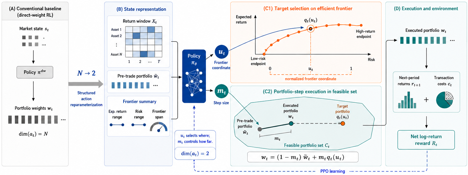Figure 1 summarizes the complete decision pipeline and contrasts the proposed two-dimensional action with direct asset-weight actions.

3.1. Problem Formulation

Consider a market containing N risky assets. Let ${\mathbf{r}}_t\in {\mathbb{R}}^N$ denote the vector of simple asset returns from time $t-1$ to time t. At each decision time t, the agent observes the information available up to that time and selects a portfolio for the next investment period.

Let ${\mathbf{w}}_{t-1}$ denote the portfolio selected at the previous decision time. After ${\mathbf{r}}_t$ is realized, price movements change the relative asset weights. The resulting pre-trade portfolio is denoted by ${\tilde{\mathbf{w}}}_t$, whose i-th element is

$${\tilde{w}}_{t,i}={\displaystyle \frac{w_{t-1,i}(1+r_{t,i})}{1+{\mathbf{w}}_{t-1}^{\top }{\mathbf{r}}_t}}.$$

(1)

We distinguish the long-only, fully invested simplex from the capped target set:

$$\begin{array}{cc}\hfill {\Delta }_N& =\left\{\mathbf{w}\in {\mathbb{R}}^N:{\mathbf{1}}^{\top }\mathbf{w}=1,\mathbf{w}\ge \mathbf{0}\right\},\hfill \\ \hfill {\mathcal{C}}_t& =\left\{\mathbf{q}\in {\Delta }_N:q_i\le w_{max}\right\}.\hfill \end{array}$$

(2)

The pre-trade portfolio remains in ${\Delta }_N$ after price drift, whereas the frontier-supported target portfolios are constructed within ${\mathcal{C}}_t$.

Direct-weight portfolio policies produce one asset-level action for each element of the investment universe. Their action dimension, therefore, increases with N, and the same action vector determines the cross-sectional allocation, the portfolio constraints, and the trading distance from the current holdings. FrontierStep-RL separates target selection from execution intensity. The frontier coordinate determines the desired risk–return position, and the rebalancing step controls the proportion of the corresponding portfolio movement. The policy is trained to maximize cumulative portfolio growth after transaction costs using only information available at or before each decision time.

3.2. Regularized Efficient-Frontier Construction

At each decision time, the expected return vector ${\widehat{\mathit{\mu }}}_t$ and covariance matrix ${\widehat{\mathbf{\Sigma }}}_t$ are estimated from a rolling historical window. Let ${\left\{{\rho }_{t,k}\right\}}_{k=1}^K$ denote prescribed target return levels within the feasible predicted-return range. Following the mean–variance principle [1], the candidate portfolio associated with ${\rho }_{t,k}$ is obtained from

$${\mathbf{q}}_{t,k}=\underset{\mathbf{q}\in {\mathcal{C}}_t}{\arg \min }\left[{\mathbf{q}}^{\top }{\widehat{\mathbf{\Sigma }}}_t\mathbf{q}+\epsilon {∥\mathbf{q}∥}_2^2\right]\mathrm{subject}\mathrm{to}{\widehat{\mathit{\mu }}}_t^{\top }\mathbf{q}\ge {\rho }_{t,k},$$

(3)

where $\epsilon >0$ is a regularization coefficient. The covariance term controls predicted portfolio variance, while the regularization term discourages excessively concentrated solutions.

The candidate portfolios are ordered by predicted return, and adjacent candidates with nearly identical weights are merged. Let $M_t\le K$ denote the number of retained frontier portfolios at decision time t. The retained sequence ${\left\{{\mathbf{q}}_{t,k}\right\}}_{k=1}^{M_t}$ provides a discrete approximation of the regularized frontier.

A point-index coordinate assigns equal intervals to consecutive candidates without accounting for the economic effect of moving between them. Euclidean arc length incorporates changes in the portfolio weights, but equal weight-space movements can produce different changes in predicted risk and transaction-cost exposure. FrontierStep-RL, therefore, parameterizes the retained frontier using local changes in predicted volatility and one-way turnover.

For the k-th retained portfolio, let ${\sigma }_{t,k}={\left({\mathbf{q}}_{t,k}^{\top }{\widehat{\mathbf{\Sigma }}}_t{\mathbf{q}}_{t,k}\right)}^{1/2}$ denote its predicted volatility. For $k=1,\dots ,M_t-1$, the local risk and turnover changes are

$${\Delta }_{t,k}^{\sigma }=\left|{\sigma }_{t,k+1}-{\sigma }_{t,k}\right|,{\Delta }_{t,k}^{\tau }={\displaystyle \frac{1}{2}}{∥{\mathbf{q}}_{t,k+1}-{\mathbf{q}}_{t,k}∥}_1.$$

(4)

Under a common proportional transaction-cost rate, ${\Delta }_{t,k}^{\tau }$ is proportional to the cost exposure associated with moving between the two portfolios.

The two components are normalized to account for their different scales. The scale factors $s_t^{\sigma }$ and $s_t^{\tau }$ are the median positive values of the corresponding local changes, lower-bounded by a numerical floor $\delta >0$. If a component has no positive local change, its scale is set to $\delta$. The local cost–risk distance is

$$d_{t,k}=\lambda {\displaystyle \frac{{\Delta }_{t,k}^{\sigma }}{s_t^{\sigma }}}+(1-\lambda ){\displaystyle \frac{{\Delta }_{t,k}^{\tau }}{s_t^{\tau }}},k=1,\dots ,M_t-1,$$

(5)

where $\lambda \in [0,1]$ controls the relative contributions of predicted risk and turnover.

The normalized coordinate of the retained frontier is defined by

$${\overline{u}}_{t,1}=0,{\overline{u}}_{t,k}={\displaystyle \frac{{\sum }_{j=1}^{k-1}{d}_{t,j}}{{\sum }_{j=1}^{M_t-1}{d}_{t,j}}},k=2,\dots ,M_t.$$

(6)

If the total distance in the denominator is numerically zero, uniformly spaced coordinates are used. Consequently, ${\overline{u}}_{t,M_t}=1$, and a frontier segment occupies a wider coordinate interval when movement across that segment produces a larger normalized change in predicted risk or turnover.

The frontier portfolios and their coordinates are constructed independently for each decision date using the information available at that date. They are cached before policy training and serve as a deterministic action-decoding structure.

3.3. Frontier-Step Action Reparameterization

The policy outputs ${\mathbf{a}}_t=(u_t,m_t)\in {[0,1]}^2$, where $u_t$ is the cost–risk-aware frontier coordinate and $m_t$ is the rebalancing step size. The coordinate selects a continuous target from the cached frontier. The endpoints satisfy ${\mathbf{q}}_t\left(0\right)={\mathbf{q}}_{t,1}$ and ${\mathbf{q}}_t\left(1\right)={\mathbf{q}}_{t,M_t}$.

For an interior coordinate, let k index two adjacent retained coordinates satisfying ${\overline{u}}_{t,k}\le u_t\le {\overline{u}}_{t,k+1}$ and ${\overline{u}}_{t,k}<{\overline{u}}_{t,k+1}$. The target portfolio is obtained by linear interpolation:

$${\mathbf{q}}_t\left(u_t\right)=(1-{\alpha }_t){\mathbf{q}}_{t,k}+{\alpha }_t{\mathbf{q}}_{t,k+1},{\alpha }_t={\displaystyle \frac{u_t-{\overline{u}}_{t,k}}{{\overline{u}}_{t,k+1}-{\overline{u}}_{t,k}}}.$$

(7)

Zero-length coordinate intervals are skipped during interpolation. Because ${\mathcal{C}}_t$ is convex, the interpolated target ${\mathbf{q}}_t\left(u_t\right)$ also belongs to ${\mathcal{C}}_t$. Values near zero select relatively conservative targets, while values near one select targets with greater exposure to the estimated return signal.

The rebalancing step determines the implemented proportion of the selected target. The executed portfolio is

$${\mathbf{w}}_t=(1-m_t){\tilde{\mathbf{w}}}_t+m_t{\mathbf{q}}_t\left(u_t\right).$$

(8)

When $m_t=0$, the pre-trade portfolio is retained. When $m_t=1$, the selected target is fully implemented. Intermediate values produce partial movement toward the target. The coordinate $u_t$, therefore, determines the target position, while $m_t$ determines the execution intensity.

Since both ${\tilde{\mathbf{w}}}_t$ and ${\mathbf{q}}_t\left(u_t\right)$ belong to ${\Delta }_N$, the executed portfolio also belongs to ${\Delta }_N$. The target portfolio additionally satisfies the asset-level cap defined by ${\mathcal{C}}_t$.

Using the standard one-way turnover definition, the executed turnover satisfies

$${\tau }_t={\displaystyle \frac{1}{2}}{∥{\mathbf{w}}_t-{\tilde{\mathbf{w}}}_t∥}_1={\displaystyle \frac{m_t}{2}}{∥{\mathbf{q}}_t\left(u_t\right)-{\tilde{\mathbf{w}}}_t∥}_1\le m_t.$$

(9)

The final inequality follows because the ${\ell }_1$ distance between two long-only, fully invested portfolios is at most two. The rebalancing step, therefore, provides an explicit upper bound on the fraction of the portfolio traded during one decision period. The policy action remains two-dimensional for every investment-universe size.

3.4. Policy Learning

A shared temporal encoder processes the rolling sequence of each asset and produces an asset-level embedding ${\mathbf{h}}_{t,i}$. The embeddings are aggregated through mean pooling, element-wise maximum pooling, and pre-trade-weighted pooling, corresponding to ${\displaystyle \frac{1}{N}}{\sum }_i{\mathbf{h}}_{t,i}$, ${max}_i{\mathbf{h}}_{t,i}$, and ${\sum }_i{\tilde{w}}_{t,i}{\mathbf{h}}_{t,i}$, respectively. Their concatenation has a fixed dimension independent of N. The pooled representation is combined with the previous portfolio return, previous turnover, and the predicted-return and risk ranges of the current frontier to form the policy state.

Because both action components lie in $[0,1]$, the policy models $u_t$ and $m_t$ with two conditional Beta distributions. Separate policy heads produce positive shape parameters for the two distributions, while a shared value head estimates the state value. Actions are sampled during training and replaced by their conditional means during evaluation.

The reward is the transaction-cost-adjusted logarithmic portfolio return:

$$R_t=\log \left[(1-c{\tau }_t)\left(1+{\mathbf{w}}_t^{\top }{\mathbf{r}}_{t+1}\right)\right],$$

(10)

where c is the all-in proportional cost per unit of one-way turnover. The reward aligns the learning objective with transaction-cost-adjusted portfolio growth. The regularized frontier and the selected coordinate define the available risk–return targets, while the step action directly controls portfolio movement.

The policy is optimized using PPO [53] with the clipped surrogate objective and generalized advantage estimation. The temporal encoder is updated jointly by the policy objective and the value objective. The policy heads are optimized through the PPO surrogate loss, while the value head is optimized through the value loss. The cached frontier serves as a deterministic decoder that maps the sampled coordinate to a target portfolio.

At each decision time, the environment updates the pre-trade portfolio, constructs the policy state, samples the two action components, decodes the selected frontier target, and applies the step-controlled allocation in Equation (8). After the next-period return is observed, the environment computes turnover, transaction cost, portfolio wealth, and the reward in Equation (10). The resulting transitions are then used for PPO updates.

4. Experimental Setup

4.1. Datasets and Evaluation Protocol

We evaluate FrontierStep-RL on three public financial datasets.FF49 contains the daily value-weighted returns of 49 U.S. industry portfolios, whereas FF100 contains 100 portfolios formed from the intersections of ten size groups and ten book-to-market groups. Both datasets are obtained from the Fama–French Data Library [54,55], and the experiments use daily observations from January 2000 to December 2025. The FF49 setting includes all 49 industry portfolios. The FF100 experiments use investment universes containing 10, 25, 50, and 100 assets. For the 10-, 25-, and 50-asset settings, five fixed stratified subsets are constructed from the $10\times 10$ size–book-to-market grid to preserve coverage across both dimensions. The subset membership is determined before model training and shared by all compared methods. The 100-asset setting uses the complete FF100 universe.

For the individual-equity evaluation, we use the stock-price component of FNSPID [56]. The 50-stock universe is constructed separately for each temporal split using only its training period. A stock is eligible when adjusted closing prices are available on at least 98% of the training-period trading days. Eligible stocks are ranked by their median daily dollar volume during the training period, and the 50 highest-ranked stocks are retained. Daily returns are computed from adjusted closing prices and aligned over the common valid trading dates of the selected stocks. We denote the resulting dataset by FNSPID-50. All experiments use an expanding-window protocol. The three training/validation/testing splits for FF49 and FF100 are 2000–2009/2010–2012/2013–2016, 2000–2013/2014–2016/2017–2020, and 2000–2017/2018–2020/2021–2025. The two splits for FNSPID-50 are 2005–2014/2015–2017/2018–2020 and 2005–2017/2018–2020/2021–2023. Feature normalization, stock-universe construction, hyperparameter selection, and checkpoint selection use the training and validation periods of the corresponding split. The test period is reserved for the final out-of-sample evaluation.

The portfolio is rebalanced daily. At decision time t, each method uses information available through that date and selects the allocation applied to the return from t to $t+1$. Every experiment starts from an equal-weight portfolio with initial wealth 1. Newly selected target allocations are long-only and fully invested, and the maximum target weight is $\min (0.20,5/N)$, where N is the number of assets. Direct-weight actions are mapped to the same capped target set before execution. The primary experiments apply a proportional transaction cost of 10 bps per unit of one-way turnover. In the transaction-cost sensitivity analysis, learning-based policies are trained under the primary 10-bps cost and evaluated at 0, 10, 25, and 50 bps. For each trained policy, the recorded test actions, gross portfolio returns, and turnover values are held fixed across the four cost assumptions, so the comparison isolates the effect of the imposed transaction cost on net performance.

4.2. Input Construction and Frontier Estimation

Each asset is represented by a 60-day sequence with four feature channels: daily simple return, five-day cumulative return, twenty-day cumulative return, and twenty-day realized volatility. Wavelet-enhanced sequence-to-sequence models provide a related approach to multi-scale short-term forecasting [57]. In the present setup, temporal scale information is represented directly through daily, five-day, and twenty-day return channels. The cumulative return over horizon h is computed as the compounded return over the preceding h trading days, and the realized-volatility channel is the standard deviation of the preceding twenty daily returns annualized by $\sqrt{252}$. The first portfolio decision in each temporal split is made after all lookback-dependent features are available. Model input features are standardized separately for each split. For each channel, the mean and standard deviation are estimated from all asset-day observations in the training period and applied unchanged to the validation and test periods. A numerical floor of ${10}^{-8}$ is applied to the standard deviation during normalization.

Expected returns are estimated from the same 60-day return window using an exponentially weighted average with decay factor $\beta =2^{-1/20}$, corresponding to a half-life of 20 trading days:

$${\widehat{\mu }}_{t,i}={\displaystyle \frac{{\sum }_{\ell =1}^{60}{\beta }^{\ell -1}{r}_{t-\ell +1,i}}{{\sum }_{\ell =1}^{60}{\beta }^{\ell -1}}}.$$

(11)

The covariance matrix is estimated from the same observations using Ledoit–Wolf shrinkage [58]. At each decision date, the lower endpoint of the target-return range is the predicted return of the capped Global Minimum Variance portfolio, and the upper endpoint is the maximum predicted return attainable within the capped target set. Forty-one target-return levels are placed at equal intervals over this range and used in the regularized frontier problem in Equation (3). The regularization coefficient is ${10}^{-4}$. Adjacent candidates with an ${\ell }_2$ distance below ${10}^{-4}$ are merged before the frontier coordinates are assigned. The cost–risk coordinate uses $\lambda =0.5$, and the numerical floor for its risk and turnover scales is $\delta ={10}^{-8}$. The convex quadratic programs are solved with absolute and relative tolerances of ${10}^{-7}$ and a maximum of 10,000 iterations. Frontier candidates, coordinates, and summary statistics are computed independently at each decision date using only preceding observations and are cached before policy training.

4.3. Baselines

We compare FrontierStep-RL with traditional portfolio strategies, controlled direct-weight RL policies, off-policy continuous-control baselines, and recent portfolio- management systems. The traditional strategies are Buy-and-Hold, Equal Weight, Global Minimum Variance, Risk Parity, and transaction-cost-aware mean–variance optimization. Buy-and-Hold starts from the equal-weight portfolio and retains the resulting drifting weights throughout each test period, whereas Equal Weight rebalances daily to $1/N$. Global Minimum Variance minimizes the estimated portfolio variance under the common long-only, full-investment, and asset-level cap constraints. Equal Weight and Global Minimum Variance provide widely used diversification benchmarks [3]. Risk Parity computes a capped equal-risk-contribution portfolio by minimizing the squared differences among asset-level risk contributions [29]; the optimization uses a convergence tolerance of ${10}^{-8}$ and at most 2000 iterations. The transaction-cost-aware mean–variance baseline, denoted by MV-TC, combines predicted return, portfolio variance, and an ${\ell }_1$ turnover penalty relative to the pre-trade portfolio. Its risk-aversion coefficient is selected from $\{0.1,0.5,1,2,5\}$, and its turnover coefficient is selected from $\{0,0.001,0.005,0.01\}$ according to validation net Sharpe ratio. All optimization-based baselines use the same expected return estimator, covariance estimator, target-weight cap, and decision dates as FrontierStep-RL.

The controlled PPO baselines are PPO-Softmax, PPO-Dirichlet, and PPO-Projection. They share the input features, temporal encoder, pooled state representation, reward, transaction cost, training budget, validation schedule, and PPO objective of FrontierStep-RL [53]. PPO-Softmax samples an N-dimensional diagonal-Gaussian latent action and converts it to a fully invested allocation through the softmax function. PPO-Dirichlet defines a distribution directly on the portfolio simplex, with positive concentration parameters obtained through a softplus transformation [27]. PPO-Projection samples an unconstrained diagonal-Gaussian action and applies Euclidean projection onto the capped simplex. Softmax and Dirichlet outputs are also projected when they violate the asset-level cap. The Gaussian policies use an initial log standard deviation of $-0.5$, which is optimized jointly with the policy, and all three PPO baselines use the conditional mean of their action distribution during evaluation. SAC-Direct applies SAC to an N-dimensional latent allocation and maps the sampled action to the capped simplex [51]. TD3-MV uses the same state representation and capped action mapping together with a risk- and transaction-cost-aware portfolio objective [16,52].

The recent portfolio-management systems are FreQuant [21], DeepAries [23], and EarnMore [22]. FreQuant retains its multi-frequency market representation, DeepAries retains its joint allocation and rebalancing-interval decisions, and EarnMore retains its maskable stock representation. EarnMore is evaluated only on FNSPID-50. The method-specific architectures and action mechanisms are retained, while the temporal splits, initial portfolios, target constraints, transaction costs, validation criterion, and test metrics follow the common protocol. Every learning-based baseline receives a budget of ${10}^6$ environment interactions. For FreQuant, DeepAries, and EarnMore, the Adam learning rate is selected from $\{{10}^{-4},3\times {10}^{-4},{10}^{-3}\}$, and the minibatch size is selected from $\{128,256\}$ according to validation performance. The selected configuration is fixed before test evaluation.

4.4. Training Configuration

FrontierStep-RL and the three controlled PPO baselines share the same state encoder and policy–value backbone. A one-layer GRU with 64 hidden units processes the 60-step, four-channel sequence of each asset. The GRU parameters are shared across assets, and the final hidden state forms a 64-dimensional asset-level embedding. Mean pooling, element-wise maximum pooling, and pre-trade-weighted pooling each produce a 64-dimensional vector. The three pooled vectors are concatenated with the previous net portfolio return, previous one-way turnover, and the minimum and maximum predicted return and volatility along the current frontier. The resulting state dimension is independent of the number of assets. The policy and value networks each contain two fully connected layers with 128 and 64 hidden units and hyperbolic-tangent activations. FrontierStep-RL uses separate output heads for the frontier coordinate and the rebalancing step. Each head produces two Beta shape parameters through $1+\mathrm{softplus}(·)$, while a linear value head produces the state-value estimate.

PPO is optimized using Adam with a constant learning rate of $3\times {10}^{-4}$, optimizer epsilon ${10}^{-5}$, and zero weight decay. Each model is trained for ${10}^6$ environment interactions. A rollout contains 2048 transitions, is divided into minibatches of 256, and is reused for ten optimization epochs. Advantages are computed using generalized advantage estimation with $\gamma =0.99$ and ${\lambda }_{\mathrm{GAE}}=0.95$ and are standardized within each optimization batch. The PPO clipping threshold is 0.20, the entropy coefficient is 0.005, the value-loss coefficient is 0.50, and the global gradient norm is clipped at 0.50.

SAC-Direct and TD3-MV use the same fixed-dimensional state representation as the PPO methods. Their actor and critic networks contain two ReLU layers with 256 hidden units. Both methods use a replay buffer containing at most ${10}^6$ transitions, a warm-up period of 10,000 interactions, a minibatch size of 256, a discount factor of 0.99, and a target-network update coefficient of 0.005. One gradient update is performed per environment interaction after the warm-up period. SAC-Direct uses actor and critic learning rates of $3\times {10}^{-4}$ and automatic entropy tuning with target entropy $-N$. TD3-MV uses an actor learning rate of ${10}^{-4}$, a critic learning rate of ${10}^{-3}$, an exploration-noise standard deviation of 0.10, and target-policy noise with standard deviation 0.20 clipped to 0.50. Its actor and target networks are updated once every two critic updates. Validation is performed every 25,000 interactions. Stochastic policies use the conditional mean of their action distribution during validation, whereas deterministic actors use their direct output. The checkpoint with the highest validation net Sharpe ratio is retained for testing. Every stochastic method is trained with random seeds 11, 23, 37, 53, and 71, and the test periods do not participate in hyperparameter or checkpoint selection.

4.5. Additional Robustness Protocols

Robustness to return and covariance estimation is evaluated on the complete 100-asset FF100 universe. The default setting combines the 60-day exponentially weighted return estimate with Ledoit–Wolf covariance. One alternative replaces the return estimate with the arithmetic mean over the same 60-day window. A second alternative retains the exponentially weighted return estimate and replaces Ledoit–Wolf covariance with the oracle-approximating shrinkage (OAS) estimator [59]. All remaining frontier, policy, training, validation, and evaluation settings are held fixed.

FrontierStep-RL and PPO-Dirichlet are evaluated on all three FF100 temporal splits with seeds 11, 37, and 71, giving nine attempted runs for each estimation setting. PPO-Dirichlet is used as the controlled direct-weight comparison because it is the strongest direct-weight policy in the primary 100-asset experiment. For PPO-Dirichlet, changing the estimator modifies the shared predicted-return and volatility summaries included in the policy state, while the policy continues to output a direct simplex-valued portfolio action. Financial metrics are aggregated over successful runs, while failures remain in the reported denominator.

The one-factor-at-a-time sensitivity analysis uses the chronologically middle FF100-100 temporal split—2000–2013 for training, 2014–2016 for validation, and 2017–2020 for testing—with seeds 11, 37, and 71. It varies the number of frontier points among 21, 41, and 81; the regularization coefficient among ${10}^{-5}$, ${10}^{-4}$, and ${10}^{-3}$; the bounded policy distribution between Beta and Logistic–Normal and the network capacity between the default 64-unit GRU with 128–64 multilayer perceptrons and a compact 32-unit GRU with 64–32 multilayer perceptrons. The Logistic–Normal variant maps Gaussian latent variables to the unit interval through a logistic transformation. All unlisted settings and the validation-based checkpoint rule remain unchanged. Sensitivity to the coordinate weight is evaluated separately using the complete 15-run Cost Only, Cost–Risk, and Risk Only comparison, corresponding to $\lambda =0$, $0.5$, and 1, respectively.

A nonlinear-friction stress test replays the recorded FF49 and FNSPID-50 test trajectories without retraining or changing portfolio actions. At impact level j, the daily execution charge is

$$C_t^{\left(j\right)}=c{\tau }_t+{\kappa }_{2,j}{\tau }_t^2\left[1+{\lambda }_j(s_t-1)\right]+{\kappa }_{3,j}{\tau }_t^3$$

(12)

where $c=0.001$. The market-stress multiplier is

$$s_t=\min \left\{3,max\left\{1,{\displaystyle \frac{{\sigma }_{t,20}^{\mathrm{mkt}}}{{\tilde{\sigma }}_{\mathrm{train},20}^{\mathrm{mkt}}}}\right\}\right\}$$

(13)

where ${\sigma }_{t,20}^{\mathrm{mkt}}$ is the 20-day realized volatility of the equal-weight return of the current investment universe, computed using information available through decision time t, and ${\tilde{\sigma }}_{\mathrm{train},20}^{\mathrm{mkt}}$ is its training-period median. The Low, Moderate, and High settings use $({\kappa }_2,{\kappa }_3,\lambda )=(0.0030,0,0)$, $(0.0075,0.0020,0.10)$, and $(0.0135,0.0070,0.23)$, respectively. For each run, the recorded portfolio weights, gross returns, and one-way turnover remain fixed; the daily net return is recomputed as $g_t^{\left(j\right)}=(1-C_t^{\left(j\right)})(1+{\mathbf{w}}_t^{\top }{\mathbf{r}}_{t+1})-1$, and the resulting run-level Sharpe ratios are aggregated over the same available evaluation runs as the primary evaluation. The same cost parameters are applied to every method and dataset.

4.6. Evaluation Metrics

Let $g_t$ denote the daily portfolio return after transaction costs:

$$g_t=(1-c{\tau }_t)\left(1+{\mathbf{w}}_t^{\top }{\mathbf{r}}_{t+1}\right)-1.$$

(14)

Annualized net return is computed as 252 times the mean daily net return, and annualized volatility is the sample standard deviation of daily net returns multiplied by $\sqrt{252}$. The net Sharpe ratio is computed from daily excess returns and annualized by $\sqrt{252}$. Daily risk-free returns are obtained from the Fama–French factor data and aligned with the trading dates of each dataset. Maximum drawdown is the largest percentage decline from a previous peak in the cumulative net wealth series. Average one-way turnover is the test-period mean of ${\tau }_t$ and is reported as a percentage per trading day.

The scalability analysis additionally reports validation learning curves, cross-run variability, and failure rates. Cross-run variability is the standard deviation of the test net Sharpe ratio across all successful combinations of temporal split, asset subset, and random seed for a given asset-universe size. FF49 contains $3\times 5=15$ stochastic runs per method, and FNSPID-50 contains $2\times 5=10$ runs. The 10-, 25-, and 50-asset FF100 settings each contain $3\times 5\times 5=75$ runs from three temporal splits, five asset subsets, and five random seeds. The complete 100-asset setting contains $3\times 5=15$ runs because it does not use subset sampling. A run is classified as failed if it produces a non-finite action, non-finite portfolio weights, a post-mapping budget-constraint error greater than ${10}^{-6}$, or a non-positive or non-finite portfolio value. Financial metrics are computed over successful runs, and failed runs are reported separately. Stochastic results are reported as the mean and standard deviation across successful runs, while deterministic baselines are aggregated across the available temporal splits and asset subsets.

5. Main Experimental Results

We organize the main experiments around six questions. First, how much do implemented portfolios, frontier targets, and rolling estimates vary across decision dates? Second, does the proposed structured action improve out-of-sample portfolio performance on both portfolio-level and individual-equity data? Third, does the fixed two-dimensional action remain effective as the number of assets increases? Fourth, does the learned step-size action improve robustness to proportional transaction costs? Fifth, does the same execution control remain effective under convex turnover-dependent costs? Sixth, does the advantage persist when either the expected-return estimator or the covariance estimator used to construct the frontier is changed? Unless otherwise stated, financial results are computed after transaction costs and reported as the mean ± standard deviation across the available evaluation runs.

5.1. Observed Time Variation in Portfolio States and Frontier Inputs

We quantify four day-to-day changes over the reported test periods. Price-induced drift is the one-way distance between the previously executed portfolio and the next pre-trade portfolio after realized returns. Fixed-coordinate target change is the one-way distance between consecutive targets decoded from the date-specific cached frontiers at coordinate $u=0.5$. Expected-return revision is the cross-asset mean absolute change in the rolling expected-return estimate, reported in basis points per day. Relative covariance revision is the Frobenius-norm change between consecutive covariance estimates divided by the Frobenius norm of the preceding estimate.

Table 1. Observed daily changes.

Dataset	Price Drift (%/day)	Target Change (%/day)	Return Revision (bps/day)	Covariance Revision (%)
FF49	0.45/0.38/0.79	2.92/2.26/5.78	1.66/1.34/3.08	2.18/1.62/4.32
FF100-100	0.41/0.28/0.91	3.84/2.18/9.36	1.55/1.02/3.72	3.06/1.85/7.82
FNSPID-50	0.76/0.54/1.62	4.51/3.37/8.84	2.78/2.05/6.18	3.54/2.63/7.14

reports the mean, median, and 90th percentile over test-period decision dates.

Price-induced drift is computed from the full FrontierStep-RL test trajectories. For each held-out date, the drift measure is first averaged across the available successful seeds within the corresponding temporal split. The fixed-coordinate target and estimator revisions are deterministic conditional on the split and date and are, therefore, computed once per split-date without seed duplication. The reported mean, median, and 90th percentile are then calculated across the resulting unique held-out dates for each dataset.

All four quantities are nonzero in every dataset. Mean price-induced drift ranges from 0.41% to 0.76% per day, whereas the target decoded at the same frontier coordinate changes by 2.92% to 4.51% per day on average. The corresponding 90th-percentile target changes reach 5.78% on FF49, 9.36% on FF100-100, and 8.84% on FNSPID-50, showing that target reconfiguration can be substantially larger than passive price drift on some decision dates.

The rolling inputs also change across consecutive dates. Mean expected-return revisions range from 1.55 to 2.78 basis points per day, and mean relative covariance revisions range from 2.18% to 3.54%. FF100-100 exhibits the largest upper-tail changes in the fixed-coordinate target and covariance estimate, while FNSPID-50 has the largest mean and median changes for most quantities. These observations provide direct empirical support for modeling portfolio management as a sequence of transitions from drifting current holdings to updated date-specific targets.

5.2. Overall Portfolio Performance

Table 2. Overall portfolio performance on FF49 at 10 bps. Results are reported as mean ± standard deviation.

Method	Ann. Net Return (%)	Volatility (%)	Net Sharpe	Max Drawdown (%)	Turnover (%/day)
Buy-and-Hold	9.3 ± 1.6	17.2 ± 1.1	0.41 ± 0.07	34.8 ± 3.6	0.00 ± 0.00
Equal Weight	9.9 ± 1.4	15.4 ± 0.9	0.49 ± 0.06	29.6 ± 2.8	0.35 ± 0.05
Global Minimum Variance	7.8 ± 0.9	10.7 ± 0.7	0.51 ± 0.05	18.9 ± 2.1	4.10 ± 0.42
Risk Parity	9.1 ± 1.0	12.7 ± 0.8	0.54 ± 0.05	21.3 ± 2.3	1.55 ± 0.22
MV-TC	10.3 ± 1.2	13.8 ± 0.9	0.58 ± 0.06	22.8 ± 2.6	1.82 ± 0.25
PPO-Softmax	10.2 ± 2.1	17.8 ± 1.6	0.45 ± 0.12	31.9 ± 4.4	11.70 ± 1.50
PPO-Dirichlet	10.9 ± 1.8	16.5 ± 1.3	0.53 ± 0.10	28.7 ± 3.8	9.60 ± 1.20
PPO-Projection	10.6 ± 1.9	16.8 ± 1.4	0.50 ± 0.11	29.5 ± 4.0	10.40 ± 1.30
SAC-Direct	10.1 ± 2.6	19.3 ± 2.0	0.41 ± 0.15	36.2 ± 5.1	13.30 ± 1.80
TD3-MV	11.3 ± 2.0	17.1 ± 1.5	0.53 ± 0.11	30.4 ± 4.0	8.70 ± 1.10
FreQuant	12.1 ± 1.7	15.8 ± 1.2	0.63 ± 0.08	25.4 ± 3.1	6.40 ± 0.80
DeepAries	12.5 ± 1.5	15.0 ± 1.1	0.69 ± 0.07	23.5 ± 2.8	4.40 ± 0.60
FrontierStep-RL	11.9 ± 1.1	12.9 ± 0.8	0.75 ± 0.05	19.8 ± 2.2	2.50 ± 0.35

and

Table 3. Overall portfolio performance on FNSPID-50 at 10 bps. Results are reported as mean ± standard deviation.

Method	Ann. Net Return (%)	Volatility (%)	Net Sharpe	Max Drawdown (%)	Turnover (%/day)
Buy-and-Hold	11.4 ± 3.2	24.6 ± 2.7	0.36 ± 0.11	45.2 ± 6.2	0.00 ± 0.00
Equal Weight	12.2 ± 2.8	21.1 ± 2.2	0.47 ± 0.10	38.4 ± 5.3	0.52 ± 0.08
Global Minimum Variance	8.9 ± 1.8	14.9 ± 1.5	0.44 ± 0.08	25.7 ± 3.7	5.10 ± 0.70
Risk Parity	10.8 ± 2.0	17.3 ± 1.7	0.49 ± 0.09	29.4 ± 4.1	2.10 ± 0.30
MV-TC	12.3 ± 2.1	18.6 ± 1.8	0.54 ± 0.09	30.8 ± 4.2	2.50 ± 0.35
PPO-Softmax	12.0 ± 3.3	24.0 ± 2.9	0.40 ± 0.14	43.5 ± 6.1	15.80 ± 2.20
PPO-Dirichlet	13.6 ± 3.0	22.1 ± 2.6	0.50 ± 0.12	38.8 ± 5.5	13.10 ± 1.90
PPO-Projection	13.1 ± 3.1	22.9 ± 2.7	0.46 ± 0.13	40.2 ± 5.8	14.00 ± 2.00
SAC-Direct	14.2 ± 4.1	26.5 ± 3.4	0.45 ± 0.16	48.0 ± 7.1	17.20 ± 2.70
TD3-MV	14.5 ± 3.3	23.2 ± 2.8	0.52 ± 0.13	40.4 ± 5.9	11.90 ± 1.60
FreQuant	15.2 ± 2.8	21.9 ± 2.4	0.59 ± 0.10	34.2 ± 4.8	8.10 ± 1.20
DeepAries	15.8 ± 2.5	20.9 ± 2.1	0.64 ± 0.09	31.6 ± 4.3	5.60 ± 0.80
EarnMore	16.1 ± 2.9	22.2 ± 2.5	0.62 ± 0.10	34.0 ± 4.7	7.20 ± 1.10
FrontierStep-RL	15.3 ± 2.0	17.5 ± 1.6	0.75 ± 0.07	27.8 ± 3.6	3.20 ± 0.50

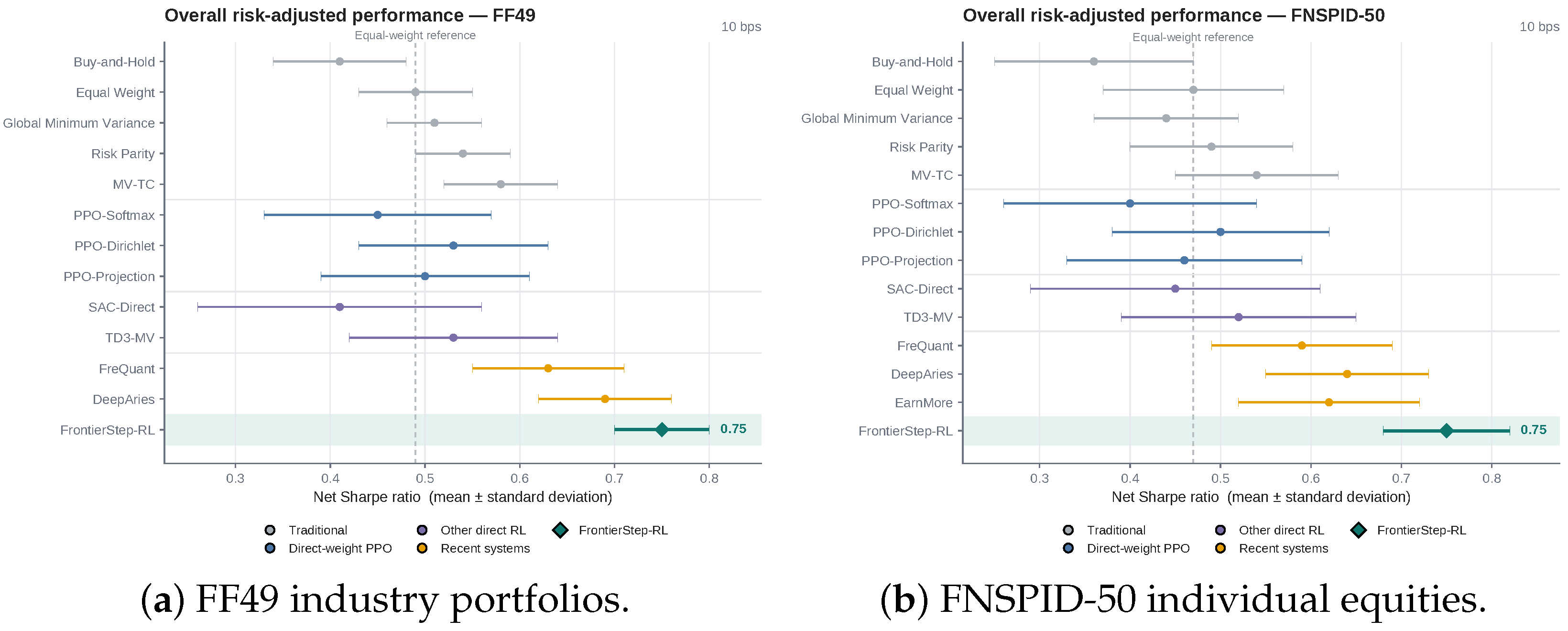
report the out-of-sample results under the primary cost of 10 bps per unit of one-way turnover. Figure 2 provides a focused comparison of the net Sharpe ratio. The markers denote the mean, and the horizontal error bars denote one standard deviation across evaluation runs.

On FF49, FrontierStep-RL achieves the highest net Sharpe ratio of $0.75\pm 0.05$. DeepAries provides the strongest competing result, at $0.69\pm 0.07$, followed by FreQuant at $0.63\pm 0.08$. FrontierStep-RL, therefore, improves the mean net Sharpe ratio over DeepAries by 8.7%. DeepAries obtains the highest annualized net return, whereas FrontierStep-RL achieves a more favorable return–risk balance. Relative to DeepAries, FrontierStep-RL reduces annualized volatility from 15.0% to 12.9%, maximum drawdown from 23.5% to 19.8%, and average daily turnover from 4.4% to 2.5%.

The FNSPID-50 results exhibit the same general pattern. FrontierStep-RL achieves a net Sharpe ratio of $0.75\pm 0.07$, compared with $0.64\pm 0.09$ for DeepAries and $0.62\pm 0.10$ for EarnMore. Although EarnMore obtains the highest annualized net return, FrontierStep-RL produces lower volatility, drawdown, and turnover than the recent learning-based baselines. Its average daily turnover is 3.2%, compared with 5.6% for DeepAries, 7.2% for EarnMore, and 8.1% for FreQuant. The consistent results on FF49 and FNSPID-50 show that the structured action performs similarly in portfolio-level and individual-equity settings.

5.3. Action-Dimension Scalability and Learning Stability

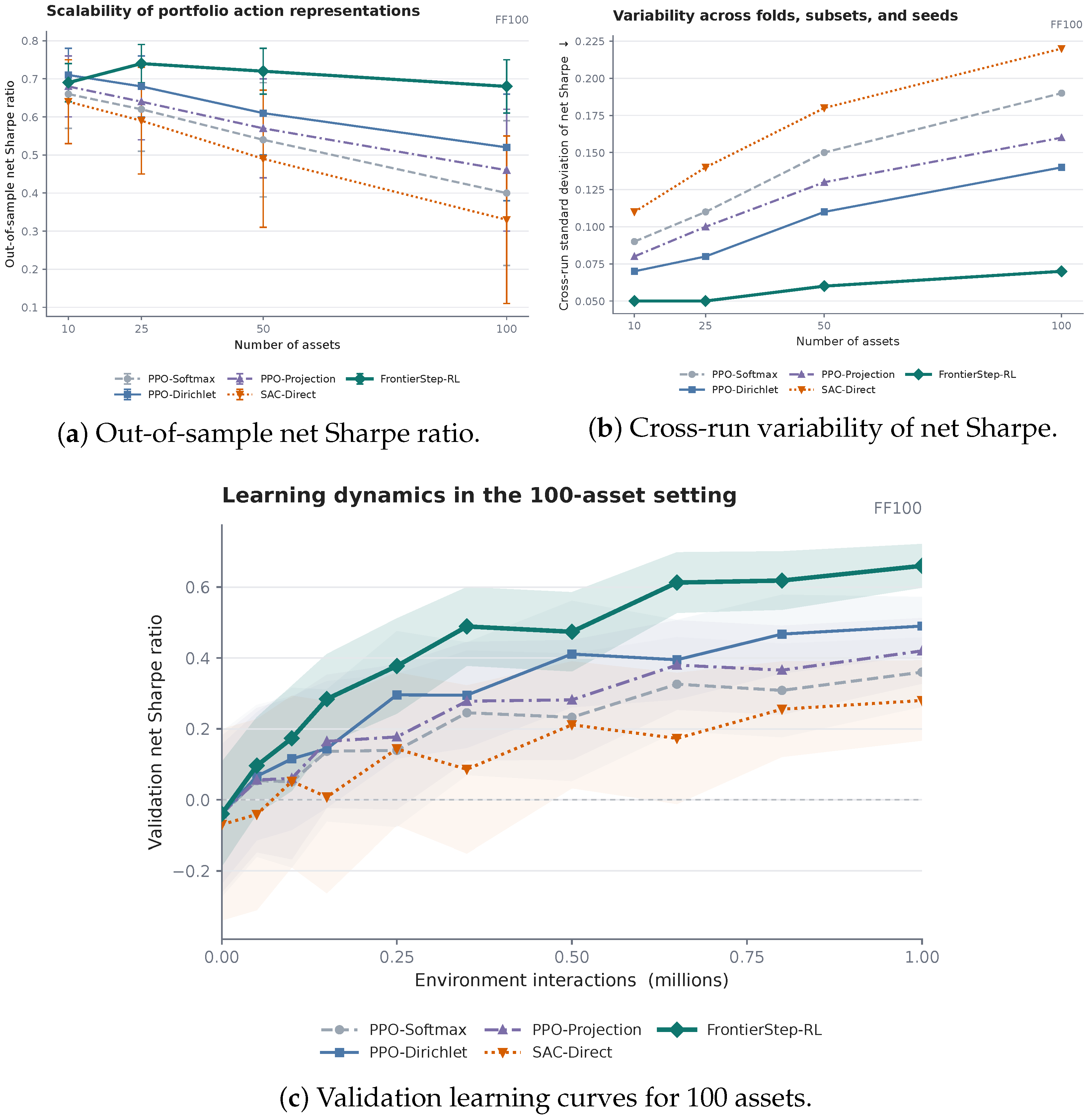
The central motivation of FrontierStep-RL is that its action dimension remains equal to two as the number of assets increases. We evaluate this property on FF100 with 10, 25, 50, and 100 assets. Figure 3 reports the out-of-sample net Sharpe ratio, the aggregate variability across runs, and the validation learning curves in the 100-asset setting.

Table 4. Action-dimension scalability on FF100. The standard deviation summarizes variability across temporal folds, asset subsets, and random seeds. Failure rates are reported explicitly because the number of runs differs between the 100-asset setting and the smaller universes.

N	Method	Net Sharpe	Cross-Run Std	Turnover (%/day)	Failure Rate
10	PPO-Softmax	0.66	0.09	7.8	0/75 (0.0%)
10	PPO-Dirichlet	0.71	0.07	6.7	0/75 (0.0%)
10	PPO-Projection	0.68	0.08	7.1	0/75 (0.0%)
10	SAC-Direct	0.64	0.11	8.5	1/75 (1.3%)
10	FrontierStep-RL	0.69	0.05	2.8	0/75 (0.0%)
25	PPO-Softmax	0.62	0.11	9.0	1/75 (1.3%)
25	PPO-Dirichlet	0.68	0.08	7.7	0/75 (0.0%)
25	PPO-Projection	0.64	0.10	8.4	1/75 (1.3%)
25	SAC-Direct	0.59	0.14	9.8	2/75 (2.7%)
25	FrontierStep-RL	0.74	0.05	2.6	0/75 (0.0%)
50	PPO-Softmax	0.54	0.15	10.4	3/75 (4.0%)
50	PPO-Dirichlet	0.61	0.11	8.8	1/75 (1.3%)
50	PPO-Projection	0.57	0.13	9.5	2/75 (2.7%)
50	SAC-Direct	0.49	0.18	11.7	5/75 (6.7%)
50	FrontierStep-RL	0.72	0.06	2.4	0/75 (0.0%)
100	PPO-Softmax	0.40	0.19	12.5	4/15 (26.7%)
100	PPO-Dirichlet	0.52	0.14	10.0	2/15 (13.3%)
100	PPO-Projection	0.46	0.16	10.8	3/15 (20.0%)
100	SAC-Direct	0.33	0.22	13.8	5/15 (33.3%)
100	FrontierStep-RL	0.68	0.07	2.2	0/15 (0.0%)

additionally reports turnover and failure rates.

With 10 assets, PPO-Dirichlet obtains a slightly higher mean net Sharpe ratio than FrontierStep-RL, at 0.71 and 0.69, respectively. FrontierStep-RL nevertheless has the lowest cross-run variability and a daily turnover of only 2.8%, compared with 6.7% for PPO-Dirichlet. As the asset universe expands, the difference in out-of-sample performance becomes more pronounced. With 25, 50, and 100 assets, FrontierStep-RL achieves net Sharpe ratios of 0.74, 0.72, and 0.68, whereas the strongest direct-weight baseline achieves 0.68, 0.61, and 0.52. The corresponding relative improvements are 8.8%, 18.0%, and 30.8%.

The variability in Figure 3b jointly summarizes temporal-fold, asset-subset, and random-seed variation and is reported as cross-run variability. FrontierStep-RL has the lowest cross-run variability among the evaluated learning-based methods at every asset-universe size. The difference is particularly clear with 100 assets, where the cross-run standard deviation is 0.07 for FrontierStep-RL and ranges from 0.14 to 0.22 for the direct-weight policies.

Failure rates provide an additional view of scalability. FrontierStep-RL completes every run successfully. In the 100-asset setting, the failure rates of PPO-Softmax, PPO-Dirichlet, PPO-Projection, and SAC-Direct are 26.7%, 13.3%, 20.0%, and 33.3%, respectively. Figure 3c further shows that FrontierStep-RL reaches stronger validation performance with a narrower uncertainty band in the largest asset universe. These results indicate that the structured two-dimensional action becomes increasingly beneficial as the direct portfolio-weight action grows in dimension.

5.4. Transaction-Cost and Turnover Robustness

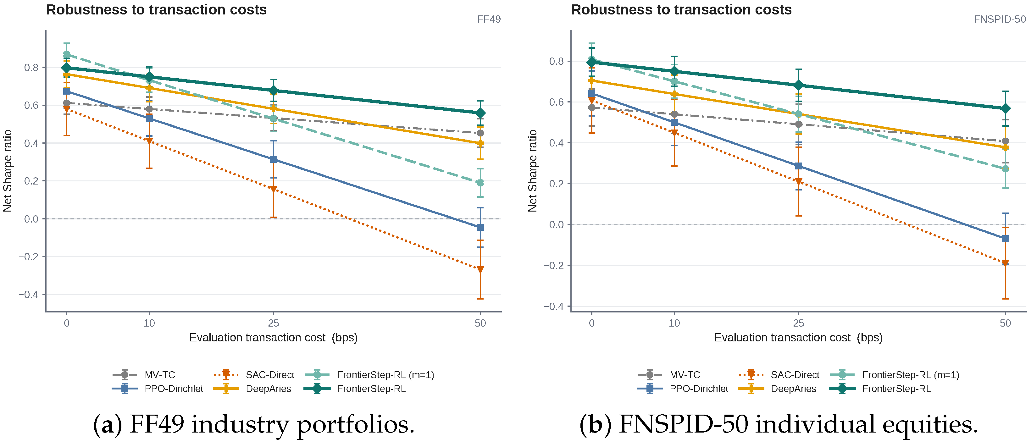
To isolate the effect of transaction costs, all learning-based policies are trained under the primary cost of 10 bps and then replayed with identical test actions under evaluation costs of 0, 10, 25, and 50 bps. The gross portfolio return and turnover of each method, therefore, remain fixed across the four evaluations, whereas the net return and net Sharpe ratio change with the imposed cost. Figure 4 reports the resulting net Sharpe ratios on FF49 and FNSPID-50.

When trading is free, the full-rebalancing variant with $m_t=1$ obtains the highest net Sharpe ratio on both datasets. On FF49, it reaches 0.868, compared with 0.798 for the adaptive-step model. On FNSPID-50, the corresponding values are 0.808 and 0.795. Cost-free execution favors immediate adoption of the selected target, while positive transaction costs increase the value of learned partial execution. At 10 bps, FrontierStep-RL obtains a net Sharpe ratio of 0.750 on both datasets, compared with 0.732 on FF49 and 0.701 on FNSPID-50 for the full-rebalancing variant.

The difference widens as the evaluation cost increases. At 50 bps, FrontierStep-RL maintains net Sharpe ratios of 0.559 on FF49 and 0.568 on FNSPID-50. The strongest competing baseline at this cost is MV-TC, with values of 0.453 and 0.408, respectively. The full-rebalancing variant decreases to 0.190 on FF49 and 0.273 on FNSPID-50. PPO-Dirichlet and SAC-Direct become negative on both datasets because their turnover remains high. In contrast, FrontierStep-RL uses average daily turnover rates of 2.5% on FF49 and 3.2% on FNSPID-50. The learned step size, therefore, preserves most of the benefit of the selected frontier target while limiting the execution cost of complete rebalancing.

Nonlinear-friction stress test. We next replay the same recorded test trajectories under the convex turnover-dependent cost in Equation (12).

Table 5. Net Sharpe under convex turnover-dependent costs.

Dataset	Method	10-bps Anchor	Low Impact	Moderate Impact	High Impact
FF49	MV-TC	$0.580\pm 0.060$	$0.578\pm 0.060$	$0.575\pm 0.061$	$0.570\pm 0.061$
	PPO-Dirichlet	$0.530\pm 0.100$	$0.466\pm 0.104$	$0.342\pm 0.120$	$0.133\pm 0.160$
	SAC-Direct	$0.410\pm 0.150$	$0.271\pm 0.146$	$-0.023\pm 0.164$	$-0.516\pm 0.242$
	DeepAries	$0.690\pm 0.070$	$0.630\pm 0.074$	$0.493\pm 0.088$	$0.242\pm 0.127$
	FrontierStep-RL ($m_t=1$)	$0.732\pm 0.063$	$0.675\pm 0.067$	$0.554\pm 0.087$	$0.339\pm 0.140$
	FrontierStep-RL	$0.750\pm 0.050$	$0.743\pm 0.050$	$0.730\pm 0.051$	$0.705\pm 0.062$
FNSPID-50	MV-TC	$0.540\pm 0.090$	$0.537\pm 0.090$	$0.532\pm 0.090$	$0.525\pm 0.090$
	PPO-Dirichlet	$0.500\pm 0.120$	$0.413\pm 0.123$	$0.242\pm 0.141$	$-0.039\pm 0.187$
	SAC-Direct	$0.450\pm 0.160$	$0.290\pm 0.156$	$-0.044\pm 0.197$	$-0.597\pm 0.329$
	DeepAries	$0.640\pm 0.090$	$0.583\pm 0.100$	$0.456\pm 0.132$	$0.226\pm 0.196$
	FrontierStep-RL ($m_t=1$)	$0.701\pm 0.083$	$0.650\pm 0.082$	$0.542\pm 0.091$	$0.353\pm 0.143$
	FrontierStep-RL	$0.750\pm 0.070$	$0.743\pm 0.071$	$0.730\pm 0.072$	$0.710\pm 0.075$

reports the net Sharpe ratio under the 10-bps proportional-cost anchor and the Low, Moderate, and High nonlinear-impact settings.

FrontierStep-RL changes only modestly under the nonlinear replay. Its net Sharpe ratio decreases from 0.750 to 0.705 on FF49 and to 0.710 on FNSPID-50 under the High setting. By comparison, the full-rebalancing variant decreases to 0.339 and 0.353, respectively. The difference shows that the learned step substantially limits exposure to convex execution costs while retaining the selected frontier target.

The higher-turnover direct-weight policies deteriorate more sharply. Under High impact, PPO-Dirichlet reaches 0.133 on FF49 and $-0.039$ on FNSPID-50, while SAC-Direct reaches $-0.516$ and $-0.597$. MV-TC changes only modestly, and DeepAries declines to 0.242 and 0.226. Because the recorded actions and gross returns are held fixed across impact settings, these differences arise from the realized turnover paths under the common nonlinear cost. The stress test, therefore, extends the proportional-cost result: learned partial execution preserves a larger share of risk-adjusted performance when execution costs increase nonlinearly with trading intensity.

5.5. Robustness to Return and Covariance Estimation

Table 6. Return- and covariance-estimator robustness on FF100-100.

Estimator	Method	Ann. Net Return (%)	Volatility (%)	Net Sharpe	Max Drawdown (%)	Turnover (%/day)	Failures
EWMA + Ledoit–Wolf	FrontierStep-RL	$11.38\pm 1.42$	$13.71\pm 0.94$	$0.684\pm 0.064$	$21.63\pm 2.58$	$2.19\pm 0.30$	0/9 (0.0%)
	PPO-Dirichlet	$10.71\pm 2.46$	$17.55\pm 1.86$	$0.519\pm 0.137$	$30.72\pm 4.31$	$9.92\pm 1.39$	1/9 (11.1%)
Rolling Mean + Ledoit–Wolf	FrontierStep-RL	$10.64\pm 1.81$	$13.98\pm 1.16$	$0.619\pm 0.097$	$23.86\pm 3.22$	$2.47\pm 0.41$	0/9 (0.0%)
	PPO-Dirichlet	$9.93\pm 2.79$	$18.21\pm 2.14$	$0.446\pm 0.164$	$33.41\pm 5.02$	$10.52\pm 1.61$	2/9 (22.2%)
EWMA + OAS	FrontierStep-RL	$11.26\pm 1.53$	$13.59\pm 1.01$	$0.675\pm 0.076$	$22.11\pm 2.90$	$2.13\pm 0.32$	0/9 (0.0%)
	PPO-Dirichlet	$10.84\pm 2.51$	$17.39\pm 1.91$	$0.532\pm 0.146$	$29.83\pm 4.47$	$9.71\pm 1.31$	1/9 (11.1%)

compares the default estimator with a rolling arithmetic-mean return estimate and an OAS covariance estimate. Each change is evaluated for both FrontierStep-RL and PPO-Dirichlet under the matched nine-run protocol described in Section 4.5.

FrontierStep-RL completes all nine runs under each estimation setting and retains a net Sharpe ratio between 0.619 and 0.684. Replacing the exponentially weighted return estimate with a rolling mean produces the clearest decline: net Sharpe falls from 0.684 to 0.619, maximum drawdown rises from 21.63% to 23.86%, and turnover rises from 2.19% to 2.47%. The OAS covariance setting remains close to the default, with net Sharpe 0.675 and turnover 2.13%.

PPO-Dirichlet continues to exhibit greater variability and higher turnover across the three settings. Its net Sharpe ranges from 0.446 to 0.532, daily turnover ranges from 9.71% to 10.52%, and one or two of nine runs fail. The relative gap between FrontierStep-RL and PPO-Dirichlet persists under both estimator changes, and the same comparative pattern appears with all three estimator settings.

Taken together, the six main analyses provide consistent evidence under the reported protocol. The descriptive results show that implemented portfolios, frontier targets, and rolling estimates vary across decision dates. FrontierStep-RL obtains strong risk-adjusted performance on the two primary evaluation datasets, shows larger relative gains as the asset universe grows, retains higher net Sharpe ratios under both proportional and convex turnover-dependent costs, and preserves its relative advantage under the two alternative estimation settings.

6. Discussion

The main experiments characterize the performance, scalability, and transaction-cost behavior of FrontierStep-RL under the reported protocol. This section first compares alternative frontier coordinate parameterizations and then evaluates sensitivity to frontier resolution, regularization, policy distribution, and network capacity. It next separates the frontier-coordinate action from the step-size action and analyzes the learned actions across market-volatility conditions. The discussion then relates these findings to existing empirical evidence, develops their theoretical and practical implications, and outlines the main limitations and research directions.

6.1. Comparison of Frontier Coordinate Parameterizations

We compare five coordinate definitions while keeping the frontier portfolios, policy architecture, step-size action, reward function, and training budget unchanged. Point Index assigns equal intervals to consecutive frontier portfolios. Euclidean Arc Length uses the cumulative ${\ell }_2$ distance between adjacent weight vectors. Risk Only and Cost Only retain only the volatility-change and turnover-change components, respectively. Cost–Risk combines the two normalized components with equal weights.

Table 7. Comparison of frontier coordinate parameterizations. Higher values are better for annualized net return and net Sharpe; lower values are better for maximum drawdown and turnover.

Dataset	Coordinate	Ann. Net Return (%) ↑	Net Sharpe ↑	Max Drawdown (%) ↓	Turnover (%/day) ↓	Failures
FF49	Point Index	11.20 ± 1.45	0.66 ± 0.08	22.60 ± 2.70	3.60 ± 0.45	0/15
	Euclidean Arc Length	11.60 ± 1.30	0.70 ± 0.07	21.20 ± 2.50	3.00 ± 0.40	0/15
	Risk Only	12.00 ± 1.25	0.73 ± 0.06	20.60 ± 2.30	3.10 ± 0.42	0/15
	Cost Only	11.30 ± 1.15	0.71 ± 0.06	19.40 ± 2.20	1.95 ± 0.30	0/15
	Cost–Risk	11.90 ± 1.10	0.75 ± 0.05	19.80 ± 2.20	2.50 ± 0.35	0/15
FF100-100	Point Index	9.60 ± 2.60	0.50 ± 0.13	30.80 ± 4.50	3.80 ± 0.60	2/15
	Euclidean Arc Length	10.50 ± 2.00	0.58 ± 0.10	27.10 ± 3.80	3.20 ± 0.50	1/15
	Risk Only	11.50 ± 1.70	0.66 ± 0.08	22.40 ± 2.90	2.90 ± 0.42	0/15
	Cost Only	10.70 ± 1.60	0.62 ± 0.08	23.20 ± 3.00	1.75 ± 0.28	0/15
	Cost–Risk	11.30 ± 1.50	0.68 ± 0.07	21.50 ± 2.70	2.20 ± 0.32	0/15

Note: Bold values indicate the best result and underlined values indicate the second-best result within each dataset. ↑ indicates that higher values are better, whereas ↓ indicates that lower values are better.

reports the out-of-sample results on FF49 and the 100-asset FF100 setting.

On FF49, Point Index produces the lowest net Sharpe ratio and the highest turnover among the five parameterizations. Euclidean Arc Length improves the net Sharpe ratio from 0.66 to 0.70 and reduces daily turnover from 3.60% to 3.00%, showing that continuity in weight space is preferable to a uniform index. The single-component coordinates reveal a clear trade-off. Risk Only obtains the highest annualized net return of 12.00%, whereas Cost Only achieves the lowest drawdown and turnover. Cost–Risk combines these properties and obtains the highest net Sharpe ratio of $0.75\pm 0.05$, while maintaining the second-lowest drawdown and turnover.

The differences become larger in the 100-asset setting. Point Index reaches a net Sharpe ratio of 0.50 and produces two failed runs, while Euclidean Arc Length reaches 0.58 with one failed run. Risk Only and Cost Only improve the result to 0.66 and 0.62, respectively, and both complete all runs. Cost–Risk achieves the strongest net Sharpe ratio of $0.68\pm 0.07$, the lowest maximum drawdown of 21.50%, and successful completion of all 15 runs. These results indicate that the economic normalization becomes more useful when the frontier spans a larger and more heterogeneous allocation space.

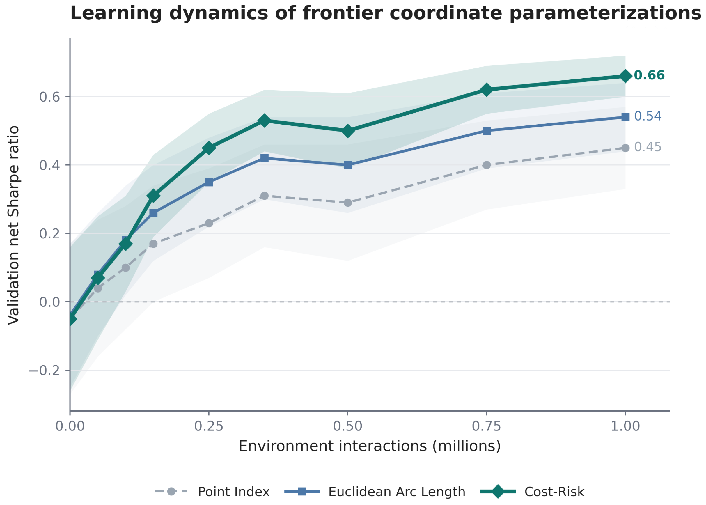
Figure 5 compares the learning dynamics of Point Index, Euclidean Arc Length, and Cost–Risk on FF100-100. The simpler coordinates improve during early training, but Cost–Risk separates from them after approximately 150,000 interactions. After one million interactions, its validation net Sharpe ratio reaches $0.66\pm 0.06$, compared with 0.54 ± 0.10 for Euclidean Arc Length and $0.45\pm 0.12$ for Point Index. The narrower uncertainty band is consistent with the lower cross-run variation in Table 7. The coordinate design, therefore, affects both the final policy and the optimization trajectory through which that policy is learned.

6.2. Hyperparameter Sensitivity

Table 8. One-factor sensitivity on the middle FF100-100 split.

Factor	Setting	Ann. Net Return (%)	Net Sharpe	Max Drawdown (%)	Turnover (%/day)	Failures
Baseline	Default	$11.22\pm 0.96$	$0.676\pm 0.054$	$21.87\pm 1.84$	$2.23\pm 0.21$	0/3 (0.0%)
Points	21	$10.73\pm 1.28$	$0.641\pm 0.073$	$23.54\pm 2.31$	$2.17\pm 0.29$	0/3 (0.0%)
	81	$11.51\pm 1.07$	$0.683\pm 0.063$	$21.62\pm 2.11$	$2.36\pm 0.33$	0/3 (0.0%)
Regularization	${10}^{-5}$	$11.57\pm 1.49$	$0.649\pm 0.086$	$24.61\pm 2.79$	$2.66\pm 0.37$	0/3 (0.0%)
	${10}^{-3}$	$10.68\pm 1.02$	$0.659\pm 0.066$	$20.93\pm 1.98$	$1.94\pm 0.24$	0/3 (0.0%)
Distribution	Logistic–Normal	$10.98\pm 1.61$	$0.635\pm 0.099$	$24.29\pm 3.16$	$2.49\pm 0.42$	0/3 (0.0%)
	GRU 32;
Architecture	MLP 64–32	$10.91\pm 1.25$	$0.658\pm 0.077$	$22.78\pm 2.49$	$2.07\pm 0.30$	0/3 (0.0%)

reports a one-factor-at-a-time sensitivity analysis under the protocol in Section 4.5. The default configuration uses 41 frontier points, regularization coefficient ${10}^{-4}$, Beta action distributions, a 64-unit GRU, and 128–64 policy and value multilayer perceptrons. Each row changes only the listed factor.

All tested local alternatives complete their three runs on the middle temporal split. Reducing the frontier from 41 to 21 points lowers net Sharpe from 0.676 to 0.641, whereas 81 points yields 0.683 with slightly higher turnover. The three frontier resolutions, therefore, produce moderate performance differences, and all complete the evaluation runs.

Regularization changes the return–risk–turnover balance. The ${10}^{-5}$ setting gives an annualized net return of 11.57%, but also the largest drawdown of 24.61% and turnover of 2.66%. The ${10}^{-3}$ setting lowers turnover to 1.94% and drawdown to 20.93%, with net Sharpe 0.659. Among the tested regularization coefficients, the default ${10}^{-4}$ setting produces the highest net Sharpe.

The Logistic–Normal and compact-network alternatives also complete every run, with net Sharpe ratios of 0.635 and 0.658, respectively, compared with 0.676 for the default. Across the tested distribution and capacity settings, performance changes remain moderate and the default obtains the highest net Sharpe. Sensitivity to the coordinate weight is reported more extensively in Table 7: Cost Only ($\lambda =0$) minimizes turnover, Risk Only ($\lambda =1$) obtains the highest annualized return, and equal Cost–Risk weighting ($\lambda =0.5$) achieves the highest net Sharpe on FF100-100.

6.3. Ablation of the Two-Dimensional Action

We next isolate the contributions of the two components in the FrontierStep-RL action. The Fixed variant uses the midpoint of the frontier, $u_t=0.5$, and fully rebalances toward this target by setting $m_t=1$. Learn $u_t$ Only dynamically selects the frontier target but fixes the step size at one. Learn $m_t$ Only fixes the target at the frontier midpoint and learns only the degree of portfolio adjustment. The Full Model jointly learns both the frontier coordinate and the step size. All variants use the same state representation, frontier candidates, reward function, training budget, and evaluation protocol. For consistency, the Full Model entries in

Table 9. Ablation of the two-dimensional action. The Full Model jointly learns the frontier coordinate $u_t$ and the step size $m_t$. Results are reported as mean ± standard deviation.

Dataset	Variant	Learn ${\mathit{u}}_{\mathit{t}}$	Learn ${\mathit{m}}_{\mathit{t}}$	Ann. Net Return (%) ↑	Net Sharpe ↑	Max Drawdown (%) ↓	Turnover (%/day) ↓
FF49	Fixed	No	No	10.10 ± 1.30	0.570 ± 0.070	24.30 ± 2.80	4.40 ± 0.55
	Learn $u_t$ Only	Yes	No	11.54 ± 1.50	0.732 ± 0.063	20.67 ± 2.43	7.00 ± 0.80
	Learn $m_t$ Only	No	Yes	10.80 ± 1.15	0.660 ± 0.060	19.30 ± 2.20	1.85 ± 0.28
	Full Model	Yes	Yes	11.90 ± 1.10	0.750 ± 0.050	19.80 ± 2.20	2.50 ± 0.35
FNSPID-50	Fixed	No	No	13.00 ± 2.50	0.510 ± 0.100	35.00 ± 4.90	5.80 ± 0.85
	Learn $u_t$ Only	Yes	No	15.53 ± 2.58	0.701 ± 0.083	27.68 ± 3.83	8.20 ± 1.10
	Learn $m_t$ Only	No	Yes	13.90 ± 2.20	0.640 ± 0.080	26.30 ± 3.60	2.55 ± 0.42
	Full Model	Yes	Yes	15.30 ± 2.00	0.750 ± 0.070	27.80 ± 3.60	3.20 ± 0.50

Note: Bold values indicate the best result and underlined values indicate the second-best result within each dataset. ↑ indicates that higher values are better, whereas ↓ indicates that lower values are better.

reuse the corresponding FrontierStep-RL results reported in Table 2 and Table 3.

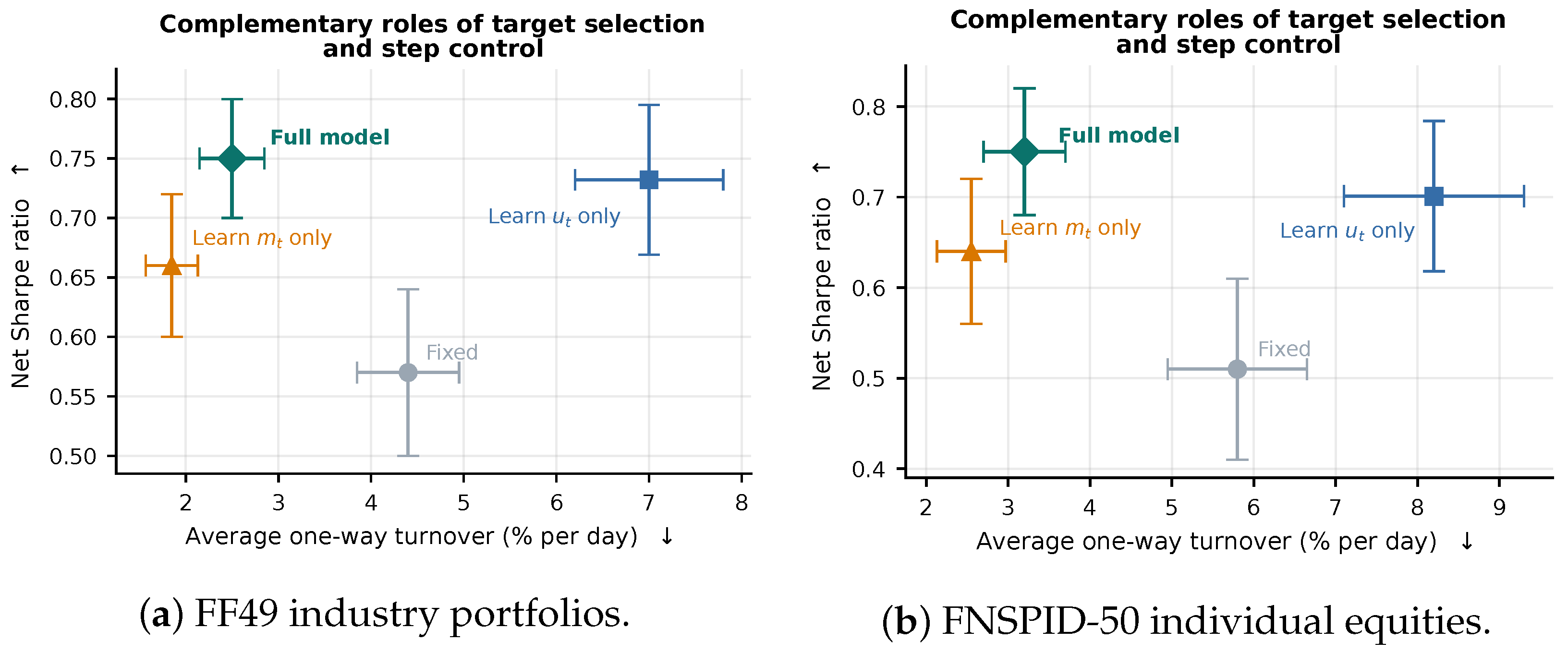
The Fixed variant produces the weakest net Sharpe ratio on both datasets, highlighting the value of state-dependent target selection and execution control. Learning only $u_t$ substantially improves annualized return and net Sharpe because the policy can dynamically select its desired risk–return position. However, setting $m_t=1$ forces the portfolio to move completely toward every selected target and, therefore, produces the highest turnover among the four variants. On FF49, Learn $u_t$ Only reaches a net Sharpe ratio of 0.732 with daily turnover of 7.00%. On FNSPID-50, it obtains the highest annualized net return of 15.53%, but its turnover increases to 8.20% per day.

Learning only $m_t$ emphasizes execution control. By adjusting the degree of movement toward a fixed midpoint target, this variant achieves the lowest turnover and maximum drawdown on both datasets. The Full Model adds state-dependent target selection and raises net Sharpe while retaining much of the execution efficiency of the step-only variant.

The Full Model combines dynamic target selection with partial portfolio execution. It achieves the highest net Sharpe ratio on both FF49 and FNSPID-50. On FF49, it also obtains the highest annualized net return while maintaining turnover close to the step-only variant. On FNSPID-50, Learn $u_t$ Only produces a slightly higher raw return, but the Full Model improves the net Sharpe ratio from 0.701 to 0.750 and reduces daily turnover from 8.20% to 3.20%. These results show that the two action components provide complementary controls: $u_t$ determines the desired position along the frontier, whereas $m_t$ regulates the extent to which the selected target is implemented.

Figure 6 provides a direct view of this complementarity. Learn $u_t$ Only moves upward in the Sharpe–turnover plane and to the right because every target is fully implemented. Learn $m_t$ Only occupies the low-turnover region, while the Full Model combines controlled turnover with the highest net Sharpe on both datasets. The joint position of the Full Model shows how dynamic target selection and controlled execution work together in FrontierStep-RL.

6.4. Behavior of the Learned Policy

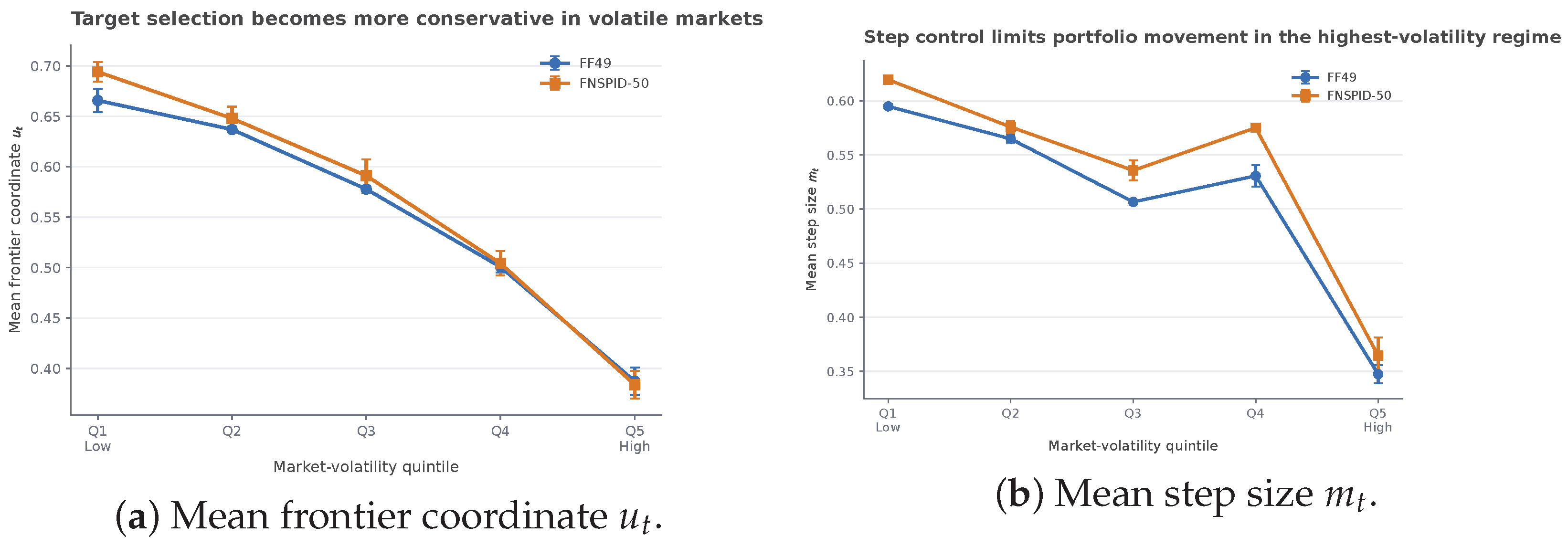
We next examine how the full policy changes its two actions across market-volatility conditions. Test observations are divided into five quintiles according to realized market volatility. Figure 7 reports the mean frontier coordinate and step size in each quintile, with error bars showing variation across temporal folds.

The frontier coordinate decreases steadily as market volatility rises. On FF49, the average $u_t$ falls from 0.666 in Q1 to 0.387 in Q5; on FNSPID-50, it falls from 0.694 to 0.384. The policy, therefore, shifts toward the conservative region of the frontier when the market becomes more volatile. The step size also declines overall, from 0.595 to 0.347 on FF49 and from 0.619 to 0.365 on FNSPID-50. Both datasets show a moderate rebound in Q4, indicating that the strategy can still undertake active reallocation during intermediate stress, followed by a marked reduction in portfolio movement under the highest-volatility condition.

Across both datasets, the two actions exhibit similar qualitative behavior: the frontier coordinate shifts the selected risk–return position, whereas the step size changes the fraction of that target implemented immediately. Under the highest-volatility condition, both actions become more conservative.

Taken together, the discussion analyses support the cost–risk-aware coordinate and the complementary roles of target selection and execution control. Their benefits are most visible in the 100-asset setting and under nonzero transaction costs, consistent with the scalability and robustness results in Section 5.

6.5. Relation to Existing Empirical Evidence

The results can be interpreted alongside established evidence that estimation error can weaken the out-of-sample performance of optimized portfolios. DeMiguel et al. show that simple diversification can remain competitive when estimation noise is substantial [3], while Petukhina et al. emphasize stabilizing estimated targets before out-of-sample evaluation [5]. FrontierStep-RL addresses a complementary part of this problem: conditional on the date-specific target set, the action representation controls how the policy searches among targets and how aggressively it implements them. The lower volatility, drawdown, and turnover observed on FF49 and FNSPID-50 indicate that implementation structure contributes to the realized return–risk trade-off in addition to enforcing feasibility.

The transaction-cost results are also consistent with dynamic trading theory. Gârleanu and Pedersen derive partial-adjustment policies that balance a moving target against trading costs [2], while Boyd et al. treat current holdings as part of multi-period portfolio decisions [9]. In the reported experiments, full rebalancing is most competitive when trading is free, whereas the learned step becomes more valuable as costs increase. The nonlinear replay strengthens this connection: under the High impact setting, the adaptive-step model retains net Sharpe ratios of 0.705 and 0.710, while the full-rebalancing variant falls to 0.339 and 0.353. This pattern connects the learned step action to the economic role of gradual portfolio adjustment.

Relative to recent portfolio RL systems, the reported comparisons make action representation a distinct empirical design dimension. FreQuant extends multi-frequency market representation [21], EarnMore supports customizable investment universes [22], and DeepAries adapts rebalancing intervals [23]. FrontierStep-RL keeps the policy action two-dimensional and delegates asset-level target construction to a financial decoder. Its empirical contribution is the observed combination of stable learning, low turnover, and an increasing relative advantage as the direct-weight action grows from 10 to 100 assets under the common evaluation protocol.

6.6. Theoretical and Practical Implications

Theoretically, the findings show that financial optimization structure can serve as a deterministic action decoder within a learned policy. The policy learns a low-dimensional decision over an ordered target family, while the decoder constructs capped target portfolios and preserves long-only, fully invested feasibility in the executed holdings. Separating the frontier coordinate from the rebalancing step also distinguishes the desired risk–return position from execution intensity, and the bound in Equation (9) gives the step action a direct portfolio-turnover interpretation. Within portfolio RL, this decomposition suggests a design principle in which a high-dimensional feasible action is represented by a structured target and an implementation fraction. For optimal portfolio construction, the optimizer defines admissible targets, while the learned step determines how fully the selected target is adopted from current holdings.

Practically, the framework preserves the same two-output policy interface as the number of assets changes. Date-specific frontier construction remains a separate computational step. The coordinate records the selected target region, and the step records the implemented fraction, making the allocation decision easier to monitor. The framework fits settings in which an institution maintains an optimizer or approved target set and seeks an adaptive rule for target selection and turnover control. The current evidence supports daily, long-only portfolio rebalancing under explicit transaction costs; higher-frequency and capacity-constrained settings motivate the execution extensions described below.

6.7. Limitations and Future Research

Several boundaries define the scope of the reported evidence. First, frontier-supported targets are generated from rolling expected-return and covariance estimates. Shrinkage and regularization improve stability, while residual estimation error remains part of target construction. Second, the represented action family is the piecewise-linear path supported by regularized frontier portfolios; broader simplex coverage would require additional target families. Third, the current evidence concerns daily, long-only, fully invested portfolios with fixed asset universes and asset-level caps. Future evaluations can extend to leverage, short selling, asset entry and exit, intraday execution, and international markets.

The experiments evaluate both proportional transaction-cost sensitivity and an exogenous convex turnover-dependent stress test. The nonlinear replay models quadratic, cubic, and volatility-scaled execution charges. Liquidity-aware extensions can add endogenous price feedback, asset-specific bid–ask spreads, order-book depth, and capacity constraints. The fixed dimension applies to the policy output; return and covariance estimation and frontier construction continue to scale with the asset universe. Future research can combine the structured action with more robust or Bayesian frontier estimators, VaR- or CVaR-based target generators, dynamic investment universes, leverage and short-sale constraints, and liquidity-aware execution models. Evaluation across additional markets and trading frequencies would further establish the conditions under which the target-and-step decomposition remains effective.

7. Conclusions

This study presented FrontierStep-RL, a structured portfolio RL framework designed to address the increasing action-space complexity of direct portfolio-weight policies. Instead of generating one action for every asset, the proposed method represents each portfolio decision through a frontier coordinate and a rebalancing step size. The regularized efficient frontier provides feasible and financially meaningful target portfolios, while the cost–risk-aware coordinate organizes these targets according to changes in predicted risk and turnover. The step-size action further separates target selection from portfolio execution and directly controls the amount of rebalancing. Consequently, the action dimension remains equal to two as the number of assets increases.

The experimental results consistently support this design. Among the compared methods, FrontierStep-RL achieves the highest net Sharpe ratio on both FF49 and FNSPID-50 while maintaining comparatively low volatility, maximum drawdown, and turnover. In the 100-asset setting, it records higher net Sharpe, lower cross-run variability and turnover, and a lower failure rate than the evaluated direct-weight RL policies. The transaction-cost experiments further show that the learned step size preserves risk-adjusted performance when execution costs increase. Coordinate comparisons and action ablations confirm that the cost–risk-aware parameterization and the two learned action components provide complementary benefits. Overall, FrontierStep-RL offers a compact and financially structured approach to scalable, cost-aware portfolio decision-making.

The estimator-robustness results further show that the relative advantage over PPO-Dirichlet persists when either the expected-return estimator or the covariance estimator is changed. The local sensitivity analysis on the middle FF100-100 split also shows that all tested frontier resolutions, regularization levels, policy distributions, and network capacities complete their runs, with moderate changes in the return–risk–turnover balance. In the nonlinear-friction replay, FrontierStep-RL retains net Sharpe ratios of 0.705 on FF49 and 0.710 on FNSPID-50 under the High setting, compared with 0.339 and 0.353 for full rebalancing. The fixed-dimensional action, therefore, provides a stable policy interface under the evaluated protocol while frontier estimation and execution frictions remain essential parts of the overall system. Its theoretical value lies in using a financially structured decoder to organize a high-dimensional feasible set, and its practical value lies in providing an interpretable target coordinate together with explicit control over rebalancing intensity. Extensions to tail-risk targets, dynamic asset universes, and liquidity-aware execution can broaden the framework beyond the present daily, long-only setting.