A Spectral Galerkin Framework for the Fractional Reaction–Subdiffusion Equation Using Legendre Cardinal Functions

Abstract

In this work, we introduce an efficient spectral Galerkin method for solving one-dimensional time-fractional reaction–subdiffusion equations. Traditional fractional operators often pose severe computational challenges and exhibit weak singularities near the initial time. To address these issues, we analytically transform the governing differential equation into a weakly singular Volterra integral equation. The numerical solution is then constructed in a two-dimensional tensor-product space using orthogonal Legendre cardinal functions on both Gauss and Gauss–Lobatto grids. A major computational advantage of this cardinal basis is that it eliminates the need for expensive numerical quadratures when assembling the operational matrices. From a theoretical view, we establish a rigorous a priori error bound and a fully computable a posteriori error estimator based on the residual. The analysis confirms that the convergence rate is governed algebraically by the Sobolev regularity of the exact solution, naturally accelerating to exponential (spectral) convergence for sufficiently smooth profiles. Extensive numerical experiments validate these theoretical claims, demonstrating that the proposed framework offers significant improvements in accuracy and efficiency.

1. Introduction

For many centuries, classical integer-order calculus was the primary tool for modeling physical processes in mathematics. However, scientists faced limitations in understanding anomalous transport phenomena. When particles move through highly porous underground rocks, become trapped inside dense biological cells, or drift in viscoelastic fluids, they do not follow the simple, predictable paths of traditional Brownian motion. Instead, they exhibit heavy-tailed waiting times and complex, long-range spatial correlations. To better capture these behaviors, researchers turned away from integer-order derivatives and began using fractional calculus. Fractional partial differential equations (FPDEs) incorporate a system’s entire history directly into the equations that describe it, providing a more accurate representation of physics that depends on memory [1,2,3]. Podlubny [4] established the foundational theory of fractional differential equations for these historical processes, while Kilbas et al. [5] expanded the core mathematical frameworks. Later, these models were successfully adapted to discrete random-walk formulations to capture anomalous transport [6].

The reaction–subdiffusion equation is one of the most important fractional partial differential equations (FPDEs) in modern applied mathematics. It describes a subtle physical balance: molecules that undergo chemical reactions at specific rates while also experiencing slow, anomalous diffusion. This type of dynamics frequently appears in environmental engineering, such as tracking groundwater contamination, or in biological contexts, like modeling the delayed spread of viral infections in heterogeneous populations [7]. Henry and Wearne [8] introduced the foundational mathematical formulations governing fractional reaction–diffusion balances, which Langlands et al. [9] subsequently extended to model multispecies linear reaction dynamics in complex biological contexts.

In this study, we address a 1D time-fractional reaction–subdiffusion problem. Our domain is continuously defined as $\Lambda \times (0,\mathcal{T}]$, with the spatial interval being $\Lambda =[a,b]$. The governing equation reads

$${\displaystyle \frac{\mathsf{\partial }w(\xi ,\tau )}{\mathsf{\partial }\tau }}={}_0\mathcal{D}_{\tau }^{1-\alpha }\left[{\displaystyle \frac{{\mathsf{\partial }}^{2}w(\xi ,\tau )}{\mathsf{\partial }{\xi }^2}}-w(\xi ,\tau )\right]+q(\xi ,\tau ),0<\alpha \le 1.$$

(1)

We pair this with a known initial condition $w(\xi ,0)=w_0\left(\xi \right)$ for $\xi \in \Lambda$, and enforce strict homogeneous Dirichlet boundaries such that $w(\xi ,\tau )=0$ on $\mathsf{\partial }\Lambda \times [0,\mathcal{T}]$ where $\mathsf{\partial }\Lambda$ indicates the spatial boundary. Here, $q(\xi ,\tau )$ is the continuous source term, and ${}_0\mathcal{D}_{\tau }^{1-\alpha }$ identifies the Riemann–Liouville fractional derivative of order $1-\alpha$.

While the physics behind this model is undeniably precise, the non-local mathematical structure effectively prevents standard numerical solvers. Since fractional operators require the entire history of the function at each time step, conventional methods quickly run into memory limitations and accumulate truncation errors. Additionally, solutions often feature a sharp, weak singularity near $\tau =0$. To overcome these computational challenges, researchers have developed a variety of localized numerical approaches. Early efforts by Yuste [10] and Murio [11] introduced weighted average and fully implicit finite difference schemes to handle fractional time-stepping. Sun and Wu [12] created a robust, fully discrete difference framework tailored to fractional diffusion-wave systems. For higher spatial resolution, Cui [13] designed a high-order compact finite difference method, while Zhuang et al. [14] introduced new analytical techniques to support implicit numerical solvers for anomalous subdiffusion. Building on these efforts, researchers have taken a closer look at adaptive frameworks and spline-based methods. For example, Maji and Natesan [15] introduced adaptive-grid techniques specifically designed for fractional boundary-value problems, while Kammappa and Awasthi [16] recently used a trigonometric cubic B-spline collocation approach to tackle time-fractional diffusion equations. Additionally, Ebrahimi et al. [17] expanded these numerical methods to solve complex inverse source problems in fractional diffusion-wave systems. Recently, researchers have introduced a wide range of advanced computational techniques to address the unique challenges posed by fractional operators. For example, local meshless collocation methods have proven highly effective for solving time-dependent fractional integral equations, including two-dimensional fractional evolution models [18]. Likewise, two-dimensional Haar wavelet methods now provide a reliable approach for handling fractional Volterra integral equations [19]. Other successful strategies include hybrid models, such as combining Laplace transforms with spectral methods to accurately simulate time-fractional wave equations [20]. Ultimately, these recent advancements reflect a shared goal within the scientific community: achieving high-order accuracy without sacrificing computational efficiency. This drive directly motivates the Legendre cardinal Galerkin framework proposed in this study. Meshless techniques are also becoming more adaptable. For instance, recent studies successfully used a local radial basis function collocation method to simulate complex, grid-free scenarios like soil collapse [21]. The mathematical theory behind these discrete fractional models is also maturing. Recent research on Liouville–Caputo fractional difference equations establishes the core existence and uniqueness proofs required to build stable numerical solvers [22].

Alternative mathematical schemes have also proven very useful. Chen et al. [23] employed a Fourier approach to model subdiffusive behavior smoothly. More recently, Dimitrov et al. [24] introduced more accurate, direct methods for approximating the Caputo derivative to better handle singular points. Finite element methods have also been carefully examined. Jin et al. [25] provided solid error estimates for semi-discrete finite element techniques applied to parabolic equations. Zeng et al. [26] combined finite difference time-stepping with finite elements to tackle fractional subdiffusion. In complex multidimensional systems, researchers have introduced creative techniques: Salama et al. [27] suggested an efficient explicit group method for advection-diffusion-reaction equations, while Abbaszadeh and Dehghan [28] avoided reliance on grids by merging an alternating direction implicit (ADI) approach with a meshless element-free Galerkin method. Galerkin methods continue to evolve for complex transient systems as well. A recent Numerov–Galerkin framework showed how coupling standard spatial projections with advanced time-stepping can accurately model the transient dynamics of anisotropic plates [29]. Finally, aiming for smooth, global approximations, Li and Xu [30] highlighted the impressive accuracy achievable with space-time spectral formulations.

However, a persistent and frustrating challenge still exists. Despite the strong push for diversity, traditional methods like finite difference, finite element, and standard ADI frameworks often completely lose their expected convergence rates when encountering that initial temporal singularity. Even when they stay stable, they tend to produce very large, ill-conditioned algebraic systems that significantly slow down the simulations.

Spectral methods are an important alternative. They offer exponential convergence for smooth profiles because they use global basis functions, making them very attractive for fractional modeling. Shen et al. [31] laid the essential mathematical groundwork for global spectral algorithms, while Zayernouri and Karniadakis [32] successfully developed specialized fractional spectral collocation techniques that leverage this exponential convergence specifically for anomalous diffusion problems. A range of specialized spectral and wavelet approaches have been carefully developed and applied to address the severe nonlocality of fractional models. Chebyshev cardinal functions have been used in pseudospectral methods for fractional Sturm–Liouville problems and for complex eigenvalue problems. In these collocation methods, the basis is built on the roots of orthogonal polynomials. This avoids the need for intensive numerical integration and for converting fractional operators into matrix representations [33,34].

Researchers have developed multiwavelet spectral element techniques to better handle sharp singularities in integral formulations. These techniques divide the computational domain into smaller, manageable elements and use localized wavelet bases, achieving high accuracy in resolving generalized Cauchy models [35]. Similarly, sparse wavelet Galerkin algorithms have been adapted to solve fractional Pantograph equations and delay differential systems. The natural sparsity of the wavelet operational matrices significantly reduces memory requirements while preserving the essential hereditary characteristics of the delayed dynamics [36,37].

In quantum mechanics and in relativistic wave equations, collocation methods using cardinal functions play a significant role. Chebyshev and Legendre cardinal expansions have been effectively used to develop accurate pseudospectral solvers for the fractional Dirac operator and the time-fractional Klein–Gordon equation [38,39]. Additionally, Legendre cardinal bases have recently shown remarkable stability when adapted for collocation schemes that tackle highly stiff fractional delay differential equations, eliminating the need for traditional numerical quadrature by leveraging the Kronecker delta property of the nodes [40].

Despite significant methodological progress, a distinct research gap remains regarding the computational overhead of standard Galerkin discretizations for subdiffusive models. Traditional finite element and spectral methods rely heavily on expensive numerical quadrature to evaluate inner products, whereas our current work directly circumvents this bottleneck. We present a new spectral Galerkin framework based on orthogonal Legendre cardinal functions. Rather than discretizing the fractional derivative directly, we use an analytical transformation that converts the differential equation into a weakly singular Volterra integral form. This approach naturally handles the initial conditions and softens the singularities near zero. By combining this integral form with the properties of Legendre cardinal basis functions, we avoid numerical quadrature during matrix assembly. The result is a robust, highly efficient algorithm that achieves spectral accuracy and overcomes many traditional computational issues associated with subdiffusive simulations.

This article is structured as follows: Section 2 details the Legendre cardinal functions and their key properties, including matrix representations of fractional integral and derivative operators. Section 3 introduces the weakly singular Volterra integral formulation and the algebraic system derived from our Galerkin method. Section 4 presents an a priori error analysis and a fully computable a posteriori error bound. Section 5 presents numerical experiments and results, and Section 6 concludes with remarks and a summary of the key findings.

2. Legendre Cardinal Functions and Operational Matrices

We are going to build and use a discrete approximation space by using Legendre cardinal functions. It is well known that, most global spectral methods need heavy numerical quadrature to find expansion coefficients, but our method avoids this by using a cardinal basis. These basis functions let us interpolate the unknown solution directly at chosen grid nodes [39,40].

For a given resolution $M\in \mathbb{N}$, we use the family of Legendre polynomials ${\left\{{\mathcal{L}}_k\right\}}_{k=0}^M$ on $[a,b]$. Their roots ${\left\{{\xi }_{k,i}\right\}}_{i=0}^{k-1}$ are real, simple, and lie strictly inside the interval [31]. Depending on how we handle boundary constraints, we generate the cardinal basis using either the Legendre–Gauss grid or the Legendre–Gauss–Lobatto grid.

2.1. Nodal Distributions and Cardinality

2.1.1. Legendre–Gauss Grid

If we do not need to enforce boundary conditions at the nodes, we build the basis using the interior roots of ${\mathcal{L}}_{M+1}$. Considering $\xi ={\displaystyle \frac{2(t-a)}{b-a}}-1$, the k-th Legendre–Gauss cardinal function is defined with standard Lagrange interpolation as follows:

$${\mathcal{B}}_k\left(\xi \right)={\displaystyle \frac{{\mathcal{L}}_{M+1}\left(\xi \right)}{\frac{d}{d\xi }\left({\mathcal{L}}_{M+1}\left({\xi }_{M+1,k}\right)\right)(\xi -{\xi }_{M+1,k})}},k=0,1,\dots ,M,\xi \in [a,b].$$

(2)

2.1.2. Legendre–Gauss–Lobatto Grid

For Dirichlet problems requiring conditions at the domain endpoints, the Gauss–Lobatto grid is optimal. It uses the extrema of ${\mathcal{L}}_M$ together with the endpoints a and b.

The Lobatto cardinal functions for these nodes are

$${\mathcal{B}}_k\left(\xi \right)={\displaystyle \frac{(1-{\xi }^2)\frac{d}{d\xi }\left({\mathcal{L}}_M\left(\xi \right)\right)}{\frac{d}{d\xi }\left((1-{\xi }_{M+1,k}^2)\frac{d}{d\xi }\left({\mathcal{L}}_M\left({\xi }_{M+1,k}\right)\right)\right)(\xi -{\xi }_{M+1,k})}},k=0,1,\dots ,M,$$

(3)

We define the node set as

$${\left\{{\xi }_{M+1,k}\right\}}_{k=0}^M:={\left\{{\widehat{\xi }}_{M,k}\right\}}_{k=0}^{M-2}\cup \{a,b\},\mathrm{where}{\displaystyle \frac{d}{d\xi }}\left({\mathcal{L}}_M\left({\widehat{\xi }}_{M,k}\right)\right)=0.$$

2.1.3. Approximation

Unlike standard orthogonal polynomial bases that require dense numerical integration for Galerkin projections, this strict cardinality acts as the primary mechanism for a completely quadrature-free matrix assembly. Regardless of the nodal distribution, this design satisfies the Kronecker delta property across the grid, ${\mathcal{B}}_k\left({\xi }_{M+1,j}\right)={\delta }_{k,j}$. As a result, any sufficiently smooth function $w\left(\xi \right)$ can be interpolated exactly. The projection onto the polynomial space is

$$w\left(\xi \right)\approx {\mathcal{P}}_M\left(w\left(\xi \right)\right)={\displaystyle \sum _{k=0}^M}w\left({\xi }_{M+1,k}\right){\mathcal{B}}_k\left(\xi \right).$$

(4)

These individual cardinal functions are assembled into a global basis vector ${\Psi }_M\left(\xi \right)\in {\mathbb{R}}^{M+1}$, where ${\left[{\Psi }_M\right]}_{k+1}\left(\xi \right)={\mathcal{B}}_k\left(\xi \right)$.

2.2. Matrix-Based Expression of the Derivative Operator

To convert the continuous derivative operator into a discrete algebraic system, the derivatives of the basis functions must be expressed in terms of themselves. This representation relies on the mathematical structure of Legendre polynomials.

The r-th derivative of the shifted Legendre polynomial is formulated as

$${\displaystyle \frac{d^r}{d{\xi }^r}}\left({\mathcal{L}}_{M+1}\right)\left(\xi \right)={\rho }_{M+1,r}{\mathcal{L}}_{M+1-r}\left(\xi \right),$$

(5)

where the scalar factor ${\rho }_{M+1,r}$ is analytically determined as [31]

$${\rho }_{M+1,r}={\displaystyle \frac{\Gamma (M+r)}{2^{r-1}(b-a)\Gamma \left(M\right)}}.$$

(6)

By applying these coefficients, we can rewrite the cardinal functions (2) and (3) in a much simpler alternative form [40]

$${\mathcal{B}}_k\left(\xi \right)=\sigma {\displaystyle \prod _{\begin{array}{c}j=0,j\ne k\end{array}}^M}(\xi -{\xi }_j),k=0,1,\dots ,M,\xi \in [a,b].$$

(7)

The scaling constant $\sigma$ that has appeared is fully determined by the selected grid configuration. If you select the Gauss grid, we obtain it as

$$\sigma ={\displaystyle \frac{{\kappa }_M}{\frac{d}{d\xi }\left({\mathcal{L}}_{M+1}\left(\xi \right)\right){|}_{\xi ={\xi }_k}}},$$

(8)

where ${\kappa }_M$ is the leading polynomial coefficient of ${\mathcal{L}}_{M+1}\left(\xi \right)$, defined as follows:

$${\kappa }_M={\displaystyle \frac{\Gamma (2M+1)}{{(b-a)}^M\Gamma {(M+1)}^2}}.$$

(9)

Similarly, if the Lobatto grid is used, the constant evaluates to

$$\sigma ={\displaystyle \frac{-4{\rho }_{M+1,1}\Gamma (2M-1)}{(M-2){(b-a)}^M\Gamma (M+1)\frac{d}{d\xi }\left((1-{\xi }^2)\frac{d}{d\xi }\left({\mathcal{L}}_M\left(\xi \right)\right)\right){|}_{\xi ={\xi }_k}}}.$$

(10)

Taking the derivative of both sides of (7), we generate the following exact summation formula

$${\displaystyle \frac{d}{d\xi }}\left({\mathcal{B}}_k\right)\left(\xi \right)=\sigma {\displaystyle \sum _{\begin{array}{c}l=0\\ l\ne k\end{array}}^M}{\displaystyle \prod _{\begin{array}{c}j=0\\ j\ne k,l\end{array}}^M}(\xi -{\xi }_j)={\displaystyle \sum _{\begin{array}{c}l=0\\ l\ne k\end{array}}^M}{\displaystyle \frac{{\mathcal{B}}_k\left(\xi \right)}{\xi -{\xi }_l}}.$$

(11)

We can then approximate this derivative by projecting it directly onto the basis functions

$${\displaystyle \frac{d}{d\xi }}\left({\mathcal{B}}_k\left(\xi \right)\right)\approx {\displaystyle \sum _{j=0}^M}{\left.{\displaystyle \frac{d}{d\xi }}\left({\mathcal{B}}_k\left(\xi \right)\right)\right|}_{\xi ={\xi }_j}{\mathcal{B}}_j\left(\xi \right).$$

(12)

By evaluating this derivative at our specified collocation points, we obtain the scalar entries needed to construct our differentiation matrix

$${\left.{\displaystyle \frac{d}{d\xi }}\left({\mathcal{B}}_k\left(\xi \right)\right)\right|}_{\xi ={\xi }_j}=\left\{\begin{array}{cc}{\displaystyle \sum _{\begin{array}{c}l=0\\ l\ne j\end{array}}^M}{\displaystyle \frac{1}{{\xi }_j-{\xi }_l}},\hfill & k=j,\hfill \\ \sigma {\displaystyle \prod _{\begin{array}{c}i=0\\ i\ne k,j\end{array}}^M}({\xi }_j-{\xi }_i),\hfill & k\ne j.\hfill \end{array}\right.$$

(13)

Using this analytical formulation directly, the derivative operator is applied to the basis vector function ${\Psi }_M\left(\xi \right)$ introduced by the dense $(M+1)\times (M+1)$ operational matrix ${\mathbf{D}}_{\xi }$. Thus, we have

$${\displaystyle \frac{d}{d\xi }}{\Psi }_M\left(\xi \right)\approx {\mathbf{D}}_{\xi }{\Psi }_M\left(\xi \right).$$

It is critical to note that because the derivative of any cardinal basis function ${\mathcal{B}}_k\left(\xi \right)\in {\Pi }_M$ is a polynomial of degree $M-1$, it remains entirely within the approximation space ${\Pi }_M$. Consequently, the interpolation of this derivative at the grid nodes introduces zero truncation error, making the discrete operational matrix ${\mathbf{D}}_{\xi }$ strictly exact for the basis functions.

2.3. Matrix-Based Expression of the Fractional Operator

Addressing the Riemann–Liouville fractional integral requires a different method. To construct the operational matrix for this operator, we need to first express the cardinal functions as a polynomial expansion. The previously mentioned product term (7) can be expanded into a power series [40]:

$${\displaystyle \prod _{\begin{array}{c}j=0\\ j\ne k\end{array}}^M}(\tau -{\tau }_j)={\displaystyle \sum _{i=0}^M}{\varrho }_{k,i}{\tau }^{M-i},$$

(14)

where we determine the weighting coefficients ${\varrho }_{k,i}$ recursively through the following relations:

$$\begin{array}{cc}\hfill {\varrho }_{k,0}& =1,{\varrho }_{k,i}={\displaystyle \frac{1}{i}}{\displaystyle \sum _{r=0}^i}{v}_{k,r}{\varrho }_{k,i-r},v_{k,r}={\displaystyle \sum _{\begin{array}{c}l=0\\ l\ne k\end{array}}^M}{\left({\tau }_l\right)}^r,k,i=0,1,\dots ,M.\hfill \end{array}$$

Consequently, any cardinal function ${\mathcal{B}}_k\left(\tau \right)$ satisfies the following clean representation:

$${\mathcal{B}}_k\left(\tau \right)=\sigma {\displaystyle \sum _{i=0}^M}{\varrho }_{k,i}{\tau }^{M-i},k=0,1,\dots ,M.$$

(15)

Now, we examine how the fractional integral applies to ${\mathcal{B}}_k\left(\tau \right)$. Assuming integration starts at zero, which perfectly matches our chosen temporal domain $(0,\mathcal{T}]$, the Riemann–Liouville fractional integral is defined as

$${\mathcal{I}}_{0+}^{\alpha }\left({\tau }^{\vartheta }\right)={\displaystyle \frac{\Gamma (\vartheta +1)}{\Gamma (\vartheta +\alpha +1)}}{\tau }^{\vartheta +\alpha },\alpha \in {\mathbb{R}}_{+}.$$

(16)

By applying this direct analytical rule directly to our expanded power series in Equation (15), we obtain the exact fractional integration of the cardinal function

$${\mathcal{I}}_{0+}^{\alpha }\left({\mathcal{B}}_k\left(\tau \right)\right)=\sigma {\displaystyle \sum _{i=0}^M}{\varrho }_{k,i}{\displaystyle \frac{\Gamma (M-i+1)}{\Gamma (M-i+\alpha +1)}}{\tau }^{M-i+\alpha }.$$

(17)

To incorporate this fractional result into our discrete collocation framework, we approximate the continuous fractional integral directly using the cardinal basis functions:

$${\mathcal{I}}_{0+}^{\alpha }\left({\mathcal{B}}_k\left(\tau \right)\right)\approx {\displaystyle \sum _{j=0}^M}{\mathcal{I}}_{0+}^{\alpha }\left({\mathcal{B}}_k\right)\left({\tau }_j\right){\mathcal{B}}_j\left(\tau \right).$$

Thanks to this calculation, we introduce the operational matrix ${\mathbf{I}}_{\alpha }\in {\mathbb{R}}^{(M+1)\times (M+1)}$. The nonlocal behavior of the operator translates perfectly into a dense algebraic array ${\mathcal{I}}_{0+}^{\alpha }\left({\Psi }_M\left(\tau \right)\right)\approx {\mathbf{I}}_{\alpha }{\Psi }_M\left(\tau \right)$, where the matrix entries are explicitly specified as

$${\left[{\mathbf{I}}_{\alpha }\right]}_{k+1,j+1}={\mathcal{I}}_{0+}^{\alpha }\left({\mathcal{B}}_k\right)\left({\tau }_j\right).$$

(18)

This operational framework enables us to efficiently calculate the impact of the fractional integral using direct matrix-vector multiplication, saving significant computational time during the discrete solver stage.

Unlike classical differentiation, the Riemann–Liouville fractional integral of a polynomial introduces fractional powers (e.g., ${\tau }^{M-i+\alpha }$), which do not inherently reside in the polynomial space ${\Pi }_M$. Therefore, while the analytical integration formula in Equation (17) is exact, the operational matrix ${\mathbf{I}}_{\alpha }$ represents an approximate $L^2$ projection of these fractional terms back onto the cardinal basis.

Remark 1.

It is well known that evaluating fractional integrals via monomial expansions (as utilized in Equations (15)–(17)) can yield matrices that are highly ill-conditioned for moderate-to-large polynomial degrees M. However, because the proposed Legendre cardinal framework achieves exponential (spectral) convergence, exceptional accuracy is attained using very small degrees (typically $M\le 15$). Consequently, the operational matrix ${\mathbf{I}}_{\alpha }$ is generated without ever entering the highly ill-conditioned regime, ensuring computational stability in standard double-precision arithmetic.

2.4. Verification for Low-Order Basis Functions

To explicitly verify the derived operational matrices, consider the lowest-order practical approximation $M=1$ on the standard spatial domain $[-1,1]$ using the Legendre–Gauss grid. The roots of ${\mathcal{L}}_2\left(\xi \right)$ yield the nodes ${\xi }_0=-1/\sqrt{3}$ and ${\xi }_1=1/\sqrt{3}$.

Using the standard interpolation formula, the exact cardinal basis functions are

$${\mathcal{B}}_0\left(\xi \right)=-{\displaystyle \frac{\sqrt{3}}{2}}\left(\xi -{\displaystyle \frac{1}{\sqrt{3}}}\right),{\mathcal{B}}_1\left(\xi \right)={\displaystyle \frac{\sqrt{3}}{2}}\left(\xi +{\displaystyle \frac{1}{\sqrt{3}}}\right).$$

(19)

By taking the first derivative of these basis functions analytically, we obtain the constant values ${\displaystyle \frac{d}{d\xi }}{\mathcal{B}}_0\left(\xi \right)=-{\displaystyle \frac{\sqrt{3}}{2}}$ and ${\displaystyle \frac{d}{d\xi }}{\mathcal{B}}_1\left(\xi \right)={\displaystyle \frac{\sqrt{3}}{2}}$. Evaluating these exact derivatives at the collocation nodes perfectly matches the proposed analytical matrix formulation in Equation (13), yielding the exact differentiation matrix:

$${\mathbf{D}}_{\xi }=\left[\begin{array}{cc}-{\displaystyle \frac{\sqrt{3}}{2}}& -{\displaystyle \frac{\sqrt{3}}{2}}\\ {\displaystyle \frac{\sqrt{3}}{2}}& {\displaystyle \frac{\sqrt{3}}{2}}\end{array}\right].$$

(20)

This confirms that the recursive derivation successfully captures the exact discrete operators without relying on numerical quadratures.

3. Spectral Galerkin Method

Here is how we transform the governing fractional partial differential equation into a Volterra integral form. Next, we will describe how to set up our solvable algebraic system using an integrated Galerkin method.

3.1. Transformation to the Volterra Equation

We rely on the fundamental relationship in calculus that connects the Riemann–Liouville fractional derivative to its corresponding integral [5]

$${}_0\mathcal{D}_{\tau }^{1-\alpha }\nu (\xi ,\tau )={\displaystyle \frac{\mathsf{\partial }}{\mathsf{\partial }\tau }}\left({\mathcal{I}}_{0+}^{\alpha }\nu (\xi ,\tau )\right).$$

(21)

Applying the first-order time integral, denoted as ${\mathcal{I}}_{0+}^1$, to the entire Equation (1) results in

$${\mathcal{I}}_{0+}^1\left({\displaystyle \frac{\mathsf{\partial }w(\xi ,\tau )}{\mathsf{\partial }\tau }}\right)={\mathcal{I}}_{0+}^1\left({\displaystyle \frac{\mathsf{\partial }}{\mathsf{\partial }\tau }}{\mathcal{I}}_{0+}^{\alpha }\left[{\displaystyle \frac{{\mathsf{\partial }}^{2}w(\xi ,\tau )}{\mathsf{\partial }{\xi }^2}}-w(\xi ,\tau )\right]\right)+{\mathcal{I}}_{0+}^{1}q(\xi ,\tau ).$$

(22)

Evaluating the left-side integral with the Fundamental Theorem of Calculus incorporates the initial condition into our main equation, while the integral remains just in front of q on the right-hand side:

$$w(\xi ,\tau )-w_0\left(\xi \right)={\mathcal{I}}_{0+}^{\alpha }\left[{\displaystyle \frac{{\mathsf{\partial }}^{2}w(\xi ,\tau )}{\mathsf{\partial }{\xi }^2}}-w(\xi ,\tau )\right]+{\mathcal{I}}_{0+}^{1}q(\xi ,\tau ).$$

(23)

Rearranging the components of this equation produces the Volterra integral equation:

$$w(\xi ,\tau )-{\mathcal{I}}_{0+}^{\alpha }{\displaystyle \frac{{\mathsf{\partial }}^{2}w(\xi ,\tau )}{\mathsf{\partial }{\xi }^2}}+{\mathcal{I}}_{0+}^{\alpha }w(\xi ,\tau )={\mathcal{I}}_{0+}^{1}q(\xi ,\tau )+w_0\left(\xi \right).$$

(24)

3.2. Galerkin Implementation via Gram Matrices

To build our fully discrete numerical model, we approximate the unknown continuous function using a two-dimensional tensor-product expansion. Using the basis vectors applied to the spatial domain, represented by ${\Psi }_M\left(\xi \right)\in {\mathbb{R}}^{(M+1)\times 1}$, and the temporal domain, represented by ${\Psi }_M\left(\xi \right)\in {\mathbb{R}}^{(M+1)\times 1}$, we express the numerical solution as

$$w_M(\xi ,\tau )={\Psi }_M^T\left(\xi \right)\mathbf{W}{\Psi }_M\left(\tau \right).$$

(25)

Since we use a cardinal basis, the matrix $\mathbf{W}\in {\mathbb{R}}^{(M+1)\times (M+1)}$ is more than just an abstract set of spectral weights. Its entries, ${\mathbf{W}}_{k,j}$, directly relate to the approximate solution values at the intersections of the spatial and temporal grids, specifically at $({\xi }_k,{\tau }_j)$.

We carefully incorporate this functional expansion into the Volterra integral equation. By translating the continuous spatial and temporal operators into the introduced discrete operational matrix forms, we obtain

$${\displaystyle \frac{{\mathsf{\partial }}^2{w}_M}{\mathsf{\partial }{\xi }^2}}\approx {\Psi }_M^T\left(\xi \right){\left({\mathbf{D}}_{\xi }^2\right)}^T\mathbf{W}{\Psi }_M\left(\tau \right),$$

and

$${\mathcal{I}}_{0+}^{\alpha }{w}_M\approx {\Psi }_M^T\left(\xi \right)\mathbf{W}{\mathbf{I}}_{\alpha }{\Psi }_M\left(\tau \right).$$

We similarly approximate the known continuous source term and initial conditions onto the grid network to create their respective $(M+1)\times (M+1)$ coefficient matrices $\mathbf{Q}$ and ${\mathbf{W}}_0$.

Substituting these approximations back into the equivalent Volterra equation allows us to define the continuous residual, ${\mathcal{R}}_M(\xi ,\tau )$, of our numerical approximation:

$${\mathcal{R}}_M(\xi ,\tau )={\Psi }_M^T\left(\xi \right)\left(\mathbf{W}-{\left({\mathbf{D}}_{\xi }^2\right)}^T\mathbf{W}{\mathbf{I}}_{\alpha }+\mathbf{W}{\mathbf{I}}_{\alpha }-\mathbf{Q}{\mathbf{I}}_1-{\mathbf{W}}_0\right){\Psi }_M\left(\tau \right).$$

(26)

To carefully minimize this error residual and identify the unknown coefficient matrix $\mathbf{W}$, we use the well-established Galerkin projection method. This reliable mathematical technique requires that the residual be exactly orthogonal to every test function within our finite-dimensional approximation space. In practical terms, this involves calculating the double integral of the residual against the product of the spatial and temporal basis functions ${\mathcal{B}}_k\left(\xi \right){\mathcal{B}}_j\left(\tau \right)$:

$${\int }_0^{\mathcal{T}}{\int }_a^b{\mathcal{R}}_M(\xi ,\tau ){\mathcal{B}}_k\left(\xi \right){\mathcal{B}}_j\left(\tau \right)d\xi d\tau =0.$$

(27)

To make this integration more relatable, we multiply the residual by the outer product of our basis vectors, ${\Psi }_M\left(\xi \right){\Psi }_M^T\left(\tau \right)$, and integrate over the entire space-time domain

$${\int }_0^{\mathcal{T}}{\int }_a^b{\Psi }_M\left(\xi \right)\left[{\Psi }_M^T\left(\xi \right)\left(\mathbf{W}-{\left({\mathbf{D}}_{\xi }^2\right)}^T\mathbf{W}{\mathbf{I}}_{\alpha }+\mathbf{W}{\mathbf{I}}_{\alpha }-\mathbf{Q}{\mathbf{I}}_1-{\mathbf{W}}_0\right){\Psi }_M\left(\tau \right)\right]{\Psi }_M^T\left(\tau \right)d\xi d\tau =0.$$

(28)

Since the algebraic coefficient matrices within the large parentheses do not depend on the variables of integration, $\xi$ and $\tau$, they can be taken outside the integrals. This allows us to define the symmetric spatial and temporal Gram matrices, known in the literature as mass matrices, denoted by ${\mathbf{G}}_{\xi }$ and ${\mathbf{G}}_{\tau }$. These $(M+1)\times (M+1)$ matrices capture the standard inner products of the cardinal basis functions in the continuous setting

$${\mathbf{G}}_{\xi }={\int }_a^b{\Psi }_M\left(\xi \right){\Psi }_M^T\left(\xi \right)d\xi ,\mathrm{and}{\mathbf{G}}_{\tau }={\int }_0^{\mathcal{T}}{\Psi }_M\left(\tau \right){\Psi }_M^T\left(\tau \right)d\tau .$$

(29)

Replacing the Gram matrices in Equation (28) reduces the original two-dimensional integral into a matrix block system

$${\mathbf{G}}_{\xi }\left(\mathbf{W}-{\left({\mathbf{D}}_{\xi }^2\right)}^T\mathbf{W}{\mathbf{I}}_{\alpha }+\mathbf{W}{\mathbf{I}}_{\alpha }-\mathbf{Q}{\mathbf{I}}_1-{\mathbf{W}}_0\right){\mathbf{G}}_{\tau }=\mathbf{0}.$$

(30)

Since Legendre cardinal functions form a set of linearly independent basis vectors, a fundamental property in functional linear algebra is that their associated Gram matrices ${\mathbf{G}}_{\xi }$ and ${\mathbf{G}}_{\tau }$ are always positive-definite and therefore invertible. By multiplying the entire relation from the left by ${\mathbf{G}}_{\xi }^{-1}$ and from the right by ${\mathbf{G}}_{\tau }^{-1}$, we can remove these mass matrices. This transforms the complicated continuous Volterra equation into an algebraic matrix equation:

$$\mathbf{W}-{\left({\mathbf{D}}_{\xi }^2\right)}^T\mathbf{W}{\mathbf{I}}_{\alpha }+\mathbf{W}{\mathbf{I}}_{\alpha }=\mathbf{Q}{\mathbf{I}}_1+{\mathbf{W}}_0.$$

(31)

Remark 2.

It is important to clarify the mathematical nature of this reduction. By introducing the continuous Gram matrices through the standard Galerkin inner product and subsequently eliminating them via multiplication by their inverses, the discrete residual is effectively forced to be identically zero at the grid nodes. Consequently, this specific Legendre cardinal Galerkin framework reduces to, and is mathematically equivalent to, a pseudospectral collocation scheme. Furthermore, if the continuous Gram matrices ${\mathbf{G}}_{\xi }$ and ${\mathbf{G}}_{\tau }$ were numerically evaluated using the exact Gauss (or Gauss–Lobatto) quadrature rules corresponding to their respective grid nodes, the strict Kronecker delta property of the cardinal basis would render them exactly diagonal. However, by analytically eliminating these mass matrices from the final algebraic system (Equation (31)), our formulation completely bypasses the need to compute, store, or invert these diagonal matrices, maximizing computational efficiency.

As a final step, the physical Dirichlet boundaries are incorporated into the algebraic system. Let the unmodified discrete system in Equation (31) be denoted as $\mathbf{A}\mathbf{W}=\mathbf{F}$, where $\mathbf{A}$ is the spatial coefficient matrix and $\mathbf{F}$ is the right-hand side matrix. The physical system demands $w(a,\tau )=0$ and $w(b,\tau )=0$. To enforce this within the discrete functional expansion, the cardinal basis vector is evaluated explicitly at the exact domain boundaries, yielding the boundary constraint vectors ${\Psi }_M^T\left(a\right)$ and ${\Psi }_M^T\left(b\right)$. The system is then modified by exactly replacing the first (index 0) and last (index M) rows of the system matrices to enforce these constraints.

The exact algebraic manipulation depends on the chosen grid:

• Legendre–Gauss–Lobatto Grid: The nodes naturally include the endpoints (${\xi }_0=a$, ${\xi }_M=b$). By the Kronecker delta property, ${\Psi }_M^T\left(a\right)=[1,0,\dots ,0]$ and ${\Psi }_M^T\left(b\right)=[0,\dots ,0,1]$. The boundary enforcement simplifies to replacing the first and last rows of $\mathbf{A}$ with exact identity constraints, and zeroing the corresponding rows of $\mathbf{F}$:

  $${\mathbf{A}}_{0,j}={\delta }_{0,j},{\mathbf{A}}_{M,j}={\delta }_{M,j},\mathrm{and}{\mathbf{F}}_{0,:}=\mathbf{0},{\mathbf{F}}_{M,:}=\mathbf{0},$$

  (32)

  where $\delta$ is the Kronecker delta.
• Legendre–Gauss Grid: The nodes are strictly interior, so the evaluated vectors ${\Psi }_M^T\left(a\right)$ and ${\Psi }_M^T\left(b\right)$ are completely dense. The PDE collocation equations at the first and last interior nodes (${\xi }_0$ and ${\xi }_M$) are sacrificed by replacing those algebraic rows in $\mathbf{A}$ with the dense boundary evaluations:

  $${\mathbf{A}}_{0,j}={\mathcal{B}}_j\left(a\right),{\mathbf{A}}_{M,j}={\mathcal{B}}_j\left(b\right),\mathrm{and}{\mathbf{F}}_{0,:}=\mathbf{0},{\mathbf{F}}_{M,:}=\mathbf{0},$$

  (33)

  for $j=0,1,\dots ,M$.

In both configurations, combining these boundary constraints with the remaining $(M-1)\times (M-1)$ interior principal submatrix preserves the full rank of the modified system, guaranteeing a uniquely solvable linear equation for the unknown matrix $\mathbf{W}$.

To find the system solution, we use the standard Gaussian elimination solver. However, if we increase the spatial and temporal resolutions to very high levels, more robust iterative algorithms like the Generalized Minimal Residual (GMRES) method can be conveniently used instead to handle the computational demands.

Remark 3.

While a rigorous theoretical proof of discrete well-posedness for this fully coupled space-time fractional Volterra system is highly complex, we operate under the standard assumption that the discrete projection inherits the well-posedness of the continuous physical operator. Specifically, because the continuous fractional reaction–subdiffusion model is rigorously known to be well-posed (see, for instance, the foundational analyses in [3,25]), we assume the resulting discrete global coefficient matrix remains strictly non-singular for a sufficiently high resolution M. Under this assumption, the orthogonal nature of the Legendre cardinal basis and the positive-definite properties of the underlying Gram matrices guarantee that the modified algebraic system yields a unique, stable solution for the unknown matrix $\mathbf{W}$.

4. A Priori and a Posteriori Error Estimates

In this section, we carefully develop a theoretical foundation that demonstrates that our numerical method consistently converges and yields reliable results. We establish an a priori error estimate to show spectral convergence, and then present a practical, fully calculable error estimate that accurately reflects the true error during implementation. Before establishing the error estimates, it is crucial to explicitly state the mathematical assumptions governing the exact solution, the fractional operator, and the forcing term. We assume the fractional order satisfies $0<\alpha <1$. Furthermore, we assume that the continuous source term $q(\xi ,\tau )$ and the initial condition $w_0\left(\xi \right)$ are sufficiently regular so that the exact solution satisfies $w(·,\tau )\in H^n(\Lambda )\cap H_0^1(\Lambda )$ for an integer $n\ge 1$ at any time $\tau \in [0,\mathcal{T}]$. The approximation space is the finite-dimensional polynomial space ${\Pi }_M$ of degree at most M.

4.1. Preliminaries and Error Decomposition

Let ${\Pi }_M$ be the finite-dimensional space of polynomials up to degree M. To better understand the spatial operators involved in the Volterra integral, we explicitly define the Ritz projection operator ${\mathcal{P}}_M:H_0^1(\Lambda )\to {\Pi }_M$, such that for any continuous test function $\nu \in H_0^1(\Lambda )$, we have

$$\langle \nabla (\nu -{\mathcal{P}}_M\nu ),\nabla {\nu }_M\rangle +\langle \nu -{\mathcal{P}}_M\nu ,{\nu }_M\rangle =0,\forall {\nu }_M\in {\Pi }_M.$$

(34)

It’s a well-established mathematical fact that for any sufficiently smooth solution $\nu \in H^n(\Lambda )\cap H_0^1(\Lambda )$, this particular Ritz projection satisfies the spectral error bound

$$\left|\right|\nu -{\mathcal{P}}_M{\nu \left|\right|}_{L^2(\Lambda )}\le C{M}^{-n}{\left|\right|\nu \left|\right|}_{H^n(\Lambda )}.$$

(35)

To better understand the overall simulation error, $e_M(\xi ,\tau )=w(\xi ,\tau )-w_M(\xi ,\tau )$, we break it down into two parts:

$$e_M={\eta }_1+{\eta }_2,$$

(36)

where ${\eta }_1=w-{\mathcal{P}}_{M}w$ denotes the projection error associated with the chosen space dimension, and ${\eta }_2={\mathcal{P}}_{M}w-w_M\in {\Pi }_M$ represents the discrete error arising from the numerical evaluation algorithm.

4.2. Semi-Discrete a Priori Spatial Error Estimate

Theorem 1.

Assume $w(\xi ,\tau )$ be the exact smooth solution to the Volterra Equation (24). Let $w_M(\xi ,\tau )\in {\Pi }_M$ be the numerical approximation obtained by the algorithm. The special discretization error $e_M(\xi ,\tau )$ satisfies the following bound for any point in time $\tau \in [0,\mathcal{T}]$:

$$\left|\right|e_M{(·,\tau )\left|\right|}_{L^2(\Lambda )}\le \mathcal{C}{M}^{-n}{\left|\right|w(·,\tau )\left|\right|}_{H^n(\Lambda )},$$

(37)

where $\mathcal{C}>0$ denotes a constant that is independent of the mesh parameter M.

Proof. 

By applying spatial integration by parts to the continuous Laplacian operator and strictly enforcing the Dirichlet boundary conditions, the exact solution w satisfies the weak Volterra equation:

$$\langle w,\nu \rangle +{\mathcal{I}}_{0+}^{\alpha }\langle \nabla w,\nabla \nu \rangle +{\mathcal{I}}_{0+}^{\alpha }\langle w,\nu \rangle =\langle {\mathcal{I}}_{0+}^{1}q,\nu \rangle +\langle w_0,\nu \rangle ,\forall \nu \in H_0^1(\Lambda ).$$

(38)

The fully discrete approximation $w_M\in {\Pi }_M$ similarly satisfies

$$\langle w_M,{\nu }_M\rangle +{\mathcal{I}}_{0+}^{\alpha }\langle \nabla w_M,\nabla {\nu }_M\rangle +{\mathcal{I}}_{0+}^{\alpha }\langle w_M,{\nu }_M\rangle =\langle {\mathcal{I}}_{0+}^{1}q,{\nu }_M\rangle +\langle w_0,{\nu }_M\rangle ,\forall {\nu }_M\in {\Pi }_M.$$

(39)

Subtracting the discrete Equation (39) from the continuous Equation (38) and directly inserting the decomposition $e_M={\eta }_1+{\eta }_2$ yields

$$\langle {\eta }_2,{\nu }_M\rangle +{\mathcal{I}}_{0+}^{\alpha }\langle \nabla {\eta }_2,\nabla {\nu }_M\rangle +{\mathcal{I}}_{0+}^{\alpha }\langle {\eta }_2,{\nu }_M\rangle =-\langle {\eta }_1,{\nu }_M\rangle -{\mathcal{I}}_{0+}^{\alpha }\left(\langle \nabla {\eta }_1,\nabla {\nu }_M\rangle +\langle {\eta }_1,{\nu }_M\rangle \right).$$

(40)

Thanks to the Ritz projection, defined in Equation (34), the entire bracket on the right-hand side vanishes. This specific Ritz projection is chosen because its orthogonality with respect to the spatial differential operator forces the bracketed terms in Equation (40) to vanish. This critical property decouples the spatial discretization error from the temporal evolution, enabling the direct application of standard polynomial approximation theory to yield the spectral error bound presented in Equation (35). Thus, the error equation collapses to

$$\langle {\eta }_2,{\nu }_M\rangle +{\mathcal{I}}_{0+}^{\alpha }\langle \nabla {\eta }_2,\nabla {\nu }_M\rangle +{\mathcal{I}}_{0+}^{\alpha }\langle {\eta }_2,{\nu }_M\rangle =-\langle {\eta }_1,{\nu }_M\rangle .$$

(41)

Setting the test function to ${\nu }_M={\eta }_2\left(\tau \right)\in {\Pi }_M$ produces the following strict energy equality:

$$\left|\right|{\eta }_2{\left(\tau \right)\left|\right|}_{L^2(\Lambda )}^2+{\mathcal{I}}_{0+}^{\alpha }\left|\right|\nabla {\eta }_2{\left(\tau \right)\left|\right|}_{L^2(\Lambda )}^2+{\mathcal{I}}_{0+}^{\alpha }\left|\right|{\eta }_2\left(\tau \right){\left|\right|}_{L^2(\Lambda )}^2=-\langle {\eta }_1\left(\tau \right),{\eta }_2\left(\tau \right)\rangle .$$

(42)

A key property of the Riemann–Liouville fractional integral is that if you have a non-negative function $\mu \left(\tau \right)\ge 0$, then its fractional integral, $I_{0+}^{\alpha }\mu \left(\tau \right)$, will always be strictly positive. When we remove the explicitly positive fractional terms from the left side of the equation, we clearly see that there is a strict upper bound as follows:

$$\left|\right|{\eta }_2\left(\tau \right){\left|\right|}_{L^2(\Lambda )}^2\le -\langle {\eta }_1\left(\tau \right),{\eta }_2\left(\tau \right)\rangle .$$

(43)

Using the Cauchy–Schwarz inequality on the right side and subsequently dividing the relation by $\left|\right|{\eta }_2\left(\tau \right){\left|\right|}_{L^2(\Lambda )}$ yields the stability bound for the discrete error

$$\left|\right|{\eta }_2{\left(\tau \right)\left|\right|}_{L^2(\Lambda )}\le \left|\right|{\eta }_1\left(\tau \right){\left|\right|}_{L^2(\Lambda )}.$$

(44)

Using the triangle inequality on the error term $e_M={\eta }_1+{\eta }_2$ gives us the bound $\left|\right|e_M{\left|\right|}_{L^2}\le 2\left|\right|{\eta }_1{\left|\right|}_{L^2}$. When we incorporate the spectral projection limit from Equation (35), we arrive at the following estimate:

$$\left|\right|e_M{(·,\tau )\left|\right|}_{L^2(\Lambda )}\le 2C{M}^{-n}{\left|\right|w(·,\tau )\left|\right|}_{H^n(\Lambda )}=\mathcal{C}{M}^{-n}{\left|\right|w(·,\tau )\left|\right|}_{H^n(\Lambda )}.$$

(45)

   □

Remark 4.

The analysis presented in Theorem 1 rigorously establishes a semi-discrete spatial error bound. In the actual computational implementation, the fully discrete tensor-product framework naturally includes a temporal discretization component arising from the time-domain cardinal projection and the interpolation-based approximation of the fractional integration matrix ${\mathbf{I}}_{\alpha }$. A comprehensive fully discrete analysis would bound the total space-time error by $O(M^{-n_{\xi }}+M^{-n_{\tau }})$, where $n_{\xi }$ and $n_{\tau }$ denote the spatial and temporal Sobolev regularities of the exact solution, respectively. Because the temporal discretization utilizes the exact same orthogonal cardinal polynomial space, the temporal projection error similarly decays exponentially for smooth profiles, justifying the overall spectral convergence observed in our numerical results.

Remark 5.

It is important to distinguish between theoretically established bounds and numerically observed behavior. Theorem 1 establishes that the theoretical convergence rate of the proposed Galerkin framework is strictly algebraic, bounded by $O\left(M^{-n}\right)$, and is fundamentally limited by the Sobolev regularity index n of the exact solution. The exponential (spectral) convergence observed later in our numerical experiments is a direct consequence of testing the algorithm against infinitely smooth exact profiles (where $n\to \infty$). For problems with lower regularity, the method will exhibit the algebraic convergence rate dictated by Theorem 1.

4.3. A Posteriori Error Estimate

While a priori bounds confirm the robust theoretical convergence rate as $M\to \infty$, practical computations benefit greatly from a posteriori error estimates. These estimates use the fully computable numerical residual to bound the physical error during the simulation.

We define the spatial residual of our discrete approximation $w_M$ as

$${\mathcal{R}}_M(\xi ,\tau )=w_M(\xi ,\tau )-{\mathcal{I}}_{0+}^{\alpha }{\displaystyle \frac{{\mathsf{\partial }}^2{w}_M(\xi ,\tau )}{\mathsf{\partial }{\xi }^2}}+{\mathcal{I}}_{0+}^{\alpha }{w}_M(\xi ,\tau )-{\mathcal{I}}_{0+}^{1}q(\xi ,\tau )-w_0\left(\xi \right).$$

(46)

It is obvious that the exact theoretical solution $w(\xi ,\tau )$ naturally produces a zero residual:

$$0=w(\xi ,\tau )-{\mathcal{I}}_{0+}^{\alpha }{\displaystyle \frac{{\mathsf{\partial }}^{2}w(\xi ,\tau )}{\mathsf{\partial }{\xi }^2}}+{\mathcal{I}}_{0+}^{\alpha }w(\xi ,\tau )-{\mathcal{I}}_{0+}^{1}q(\xi ,\tau )-w_0\left(\xi \right).$$

(47)

Subtracting (47) from (46) and invoking the definition of the global error, $e_M=w-w_M$, yields the following residual equation:

$$-{\mathcal{R}}_M(\xi ,\tau )=e_M(\xi ,\tau )-{\mathcal{I}}_{0+}^{\alpha }{\displaystyle \frac{{\mathsf{\partial }}^2{e}_M(\xi ,\tau )}{\mathsf{\partial }{\xi }^2}}+{\mathcal{I}}_{0+}^{\alpha }{e}_M(\xi ,\tau ).$$

(48)

By taking the inner product with $e_M\left(\tau \right)$ and applying spatial integration by parts, we obtain

$$-\langle {\mathcal{R}}_M\left(\tau \right),e_M\left(\tau \right)\rangle =\left|\right|e_M{\left(\tau \right)\left|\right|}_{L^2(\Lambda )}^2+{\mathcal{I}}_{0+}^{\alpha }\left|\right|\nabla e_M{\left(\tau \right)\left|\right|}_{L^2(\Lambda )}^2+{\mathcal{I}}_{0+}^{\alpha }\left|\right|e_M\left(\tau \right){\left|\right|}_{L^2(\Lambda )}^2.$$

(49)

Taking into account the positivity of the Riemann–Liouville fractional integral applied to the non-negative squared norms, we can neglect the two fractional terms on the right-hand side to obtain the following inequality:

$$\left|\right|e_M\left(\tau \right){\left|\right|}_{L^2(\Lambda )}^2\le -\langle {\mathcal{R}}_M\left(\tau \right),e_M\left(\tau \right)\rangle .$$

(50)

Applying the Cauchy–Schwarz inequality leads to

$$\left|\right|e_M{\left(\tau \right)\left|\right|}_{L^2(\Lambda )}^2\le \left|\right|{\mathcal{R}}_M{\left(\tau \right)\left|\right|}_{L^2(\Lambda )}\left|\right|e_M\left(\tau \right){\left|\right|}_{L^2(\Lambda )}.$$

(51)

Finally, dividing the expression by $\left|\right|e_M\left(\tau \right){\left|\right|}_{L^2(\Lambda )}$ yields a computable a posteriori bound:

$$\left|\right|e_M{(·,\tau )\left|\right|}_{L^2(\Lambda )}\le \left|\right|{\mathcal{R}}_M(·,\tau ){\left|\right|}_{L^2(\Lambda )}.$$

(52)

This shows that at any point in time, the overall $L^2$ error produced by the numerical scheme is less than or equal to the $L^2$ norm of the current computational residual.

To rigorously evaluate the accuracy of the numerical approximation, an a posteriori error estimator is introduced. By definition, an estimator is termed “computable” if it can be evaluated entirely using known quantities, namely, the computed numerical solution, the basis functions, and the problem’s source data, without requiring any knowledge of the true analytical solution.

Because the proposed Legendre cardinal framework mathematically reduces to a collocation scheme, the discrete residual is identically zero at the exact computational grid nodes (up to machine precision). Consequently, evaluating the residual using the discrete interpolation-based operational matrix ${\mathbf{I}}_{\alpha }$ would falsely yield a zero error. Therefore, in practice, the a posteriori residual is evaluated continuously. The numerical approximation is substituted back into the original fractional PDE, and the exact Riemann–Liouville (RL) integrals are computed analytically using continuous Gamma function formulations. The $L_2$-norm of this continuous spatial residual is then measured using a high-order (100-point) Gaussian quadrature rule. This densely samples the domain, accurately capturing the non-zero inter-nodal continuous error.

The quality of this estimator is assessed through its reliability and its effectivity index. The estimator is considered “reliable” if it provides a guaranteed upper bound on the true error, mathematically satisfying $\parallel e\parallel \le C\eta$ for a constant $C>0$, where e is the exact error and $\eta$ is the estimated residual. The sharpness of this bound is measured by the effectivity index, defined as the ratio of the estimated error to the true error ($EI=\eta /\parallel e\parallel$).

5. Numerical Experiments

Before sharing the experimental results, we describe the computational environment, the steps of our algorithm, and the mathematical ways we used to measure how well our framework works.

To rigorously quantify the accuracy of the Legendre cardinal Galerkin scheme, we measure the deviation between the exact analytical solution $w(\xi ,\tau )$ and our numerical approximation $w_M(\xi ,\tau )$. Throughout these experiments, we track both the global continuous $L^2$-norm and the discrete maximum $L^{\infty }$-norm over the space-time grid. These error metrics are defined as follows:

$$E_2={\left({\int }_0^{\mathcal{T}}{\int }_a^b|w(\xi ,\tau )-w_M(\xi ,\tau ){|}^{2}d\xi d\tau \right)}^{1/2},$$

(53)

$$E_{\infty }=\underset{\begin{array}{c}0\le i\le M\\ 0\le j\le M\end{array}}{max}|w({\xi }_i,{\tau }_j)-w_M({\xi }_i,{\tau }_j)|.$$

(54)

To quantitatively evaluate the reliability of the proposed a posteriori error estimator, we define the Effectivity Index (EI) as the ratio of the computable residual bound to the actual error, specifically $EI={\left|\right|{\mathcal{R}}_M\left|\right|}_{L^2}/E_2$. An estimator is theoretically reliable if $EI\ge 1$ and computationally highly efficient when the index remains tightly bounded near 1.

For absolute clarity and reproducibility, the end-to-end numerical implementation of our method is summarized in Algorithm 1.

Algorithm 1 Spectral Galerkin Method via Legendre Cardinal Functions

Grid Initialization: Define the required space-time resolution M and generate the discrete nodal network ${\left\{{\xi }_i\right\}}_{i=0}^M$ and ${\left\{{\tau }_j\right\}}_{j=0}^M$ using either the Legendre–Gauss or Legendre–Gauss–Lobatto roots. Basis Construction: Assemble the spatial and temporal cardinal basis vectors ${\Psi }_M\left(\xi \right)$ and ${\Psi }_M\left(\tau \right)$ using the exact interpolation formulas. Operational Matrices: Analytically compute the spatial differentiation matrix ${\mathbf{D}}_{\xi }$ and the Riemann–Liouville fractional integration matrix ${\mathbf{I}}_{\alpha }$ based on the selected grid. System Assembly: Evaluate the continuous source term $q(\xi ,\tau )$ and the initial physical state $w_0\left(\xi \right)$ at the grid nodes to populate the discrete coefficient matrices $\mathbf{Q}$ and ${\mathbf{W}}_0$. Algebraic Formulation: Construct the core algebraic system $\mathbf{W}-{\left({\mathbf{D}}_{\xi }^2\right)}^T\mathbf{W}{\mathbf{I}}_{\alpha }+\mathbf{W}{\mathbf{I}}_{\alpha }=\mathbf{Q}{\mathbf{I}}_1+{\mathbf{W}}_0$. Boundary Enforcement: Overwrite the first and last rows of the left and right-hand side matrices to definitively lock in the physical Dirichlet constraints. Solution Extraction: Solve the resulting dense linear system via Gaussian elimination to extract the unknown spectral coefficient matrix $\mathbf{W}$, which directly yields the approximate values at the grid nodes.

Regarding the computational setup, all mathematical routines, matrix assemblies, and numerical simulations discussed in this section were executed on a personal computer equipped with an Intel Core i7-6700K CPU running at 4.00 GHz and 8 GB of RAM, utilizing the Maple 2022 and MATLAB R2022a software environments.

Example 1.

The continuous transport process is governed by the following fractional partial differential equation:

$${\displaystyle \frac{\mathsf{\partial }w(\xi ,\tau )}{\mathsf{\partial }\tau }}={}_0\mathcal{D}_{\tau }^{1-\alpha }\left[{\displaystyle \frac{1}{{\pi }^8}}{\displaystyle \frac{{\mathsf{\partial }}^{2}w(\xi ,\tau )}{\mathsf{\partial }{\xi }^2}}-{\displaystyle \frac{{\alpha }^2}{4}}w(\xi ,\tau )\right]+q(\xi ,\tau ),(\xi ,\tau )\in [0,1]\times (0,1].$$

(55)

with homogeneous Dirichlet boundaries at both ends of the spatial interval

$$w(0,\tau )=0,w(1,\tau )=0,\tau \in [0,1],$$

and the initial condition

$$w(\xi ,0)=0,\xi \in [0,1].$$

Here the analytical continuous source term $q(\xi ,\tau )$ is defined as

$$\begin{array}{cc}\hfill q(\xi ,\tau )=2\tau {\xi }^2{(1-\xi )}^2(& {\xi }^2{(1-\xi )}^2\left(1+{\displaystyle \frac{{\alpha }^2{\tau }^{\alpha }}{4\Gamma (2+\alpha )}}\right)-{\displaystyle \frac{4{\tau }^{\alpha }}{{\pi }^8\Gamma (2+\alpha )}}(14{\xi }^2-14\xi +3)).\hfill \end{array}$$

(56)

This subdiffusion problem admits the following exact solution [41]:

$$w(\xi ,\tau )={\tau }^2{\xi }^4{(1-\xi )}^4.$$

(57)

To verify the practical performance of our spectral framework, we evaluated Example 1 at different space-time resolutions, taking $\alpha =0.5$. As shown in

Table 1. The maximum absolute errors ($E_{\infty }$) evaluated with different M values for Example 1.

	Gauss Grid			Lobatto Grid
$\mathit{\tau }\setminus \mathit{M}$	9	13	15	9	13	15
$0.1$	1.16 × 10−10	1.69 × 10−10	4.00 × 10−11	8.07 × 10−10	2.08 × 10−11	2.02 × 10−10
$0.2$	9.91 × 10−10	1.53 × 10−11	5.66 × 10−11	3.88 × 10−10	2.93 × 10−10	5.18 × 10−11
$0.3$	1.32 × 10−10	1.17 × 10−10	1.41 × 10−11	3.03 × 10−9	8.58 × 10−12	2.14 × 10−10
$0.4$	1.32 × 10−10	2.32 × 10−11	5.14 × 10−11	2.34 × 10−9	4.34 × 10−10	2.17 × 10−11
$0.5$	7.26 × 10−10	1.02 × 10−10	2.02 × 10−11	2.15 × 10−10	2.03 × 10−12	1.70 × 10−10
$0.6$	5.07 × 10−10	5.21 × 10−11	4.54 × 10−11	3.81 × 10−10	2.20 × 10−10	3.57 × 10−11
$0.7$	5.52 × 10−11	6.73 × 10−11	2.29 × 10−11	2.56 × 10−9	2.67 × 10−10	1.15 × 10−10
$0.8$	5.44 × 10−10	7.33 × 10−11	4.74 × 10−11	1.62 × 10−9	5.55 × 10−11	5.54 × 10−11
$0.9$	4.60 × 10−10	8.12 × 10−11	2.00 × 10−11	2.56 × 10−10	2.62 × 10−10	1.43 × 10−10
$1.0$	1.44 × 10−9	2.01 × 10−10	9.33 × 10−11	1.26 × 10−9	1.80 × 10−10	8.51 × 10−11
CPU time	$0.938$	$6.016$	$16.797$	$0.766$	$5.937$	$17.047$

, higher polynomial degrees give smaller maximum absolute errors with acceptable CPU times. To rigorously compare the proposed method with established numerical approaches,

Table 2. Comparison of total degrees of freedom (DOFs) and $E_{\infty }$ error for Example 1 with existing meshless methods [41].

Method	Total DOFs	${\mathit{E}}_{\mathit{\infty }}$ Error
Meshless method with $h=1/2,\tau =1/4$	≈15	1.86 × 10−3
Meshless method with $h=1/4,\tau =1/8$	≈45	4.26 × 10−4
Meshless method with $h=1/8,\tau =1/16$	≈153	2.16 × 10−5
Presented Method with Gauss grid ($M=9$)	100	1.44 × 10−9
Presented Method with Lobatto grid ($M=9$)	100	3.03 × 10−9

presents a head-to-head comparison of our framework and the meshless method [41] using the same test problem and parameter settings. Rather than comparing error values alone, we assess computational complexity by the total degrees of freedom (DOFs). The meshless method exhibits an algebraic convergence rate, requiring more DOFs to reduce the error incrementally. In contrast, the proposed method’s spectral convergence rate achieves a maximum error of $O\left({10}^{-9}\right)$ with only 100 total DOFs. Combined with the minimal CPU times reported in Table 1, this dramatic reduction in system size demonstrates vastly superior computational efficiency.

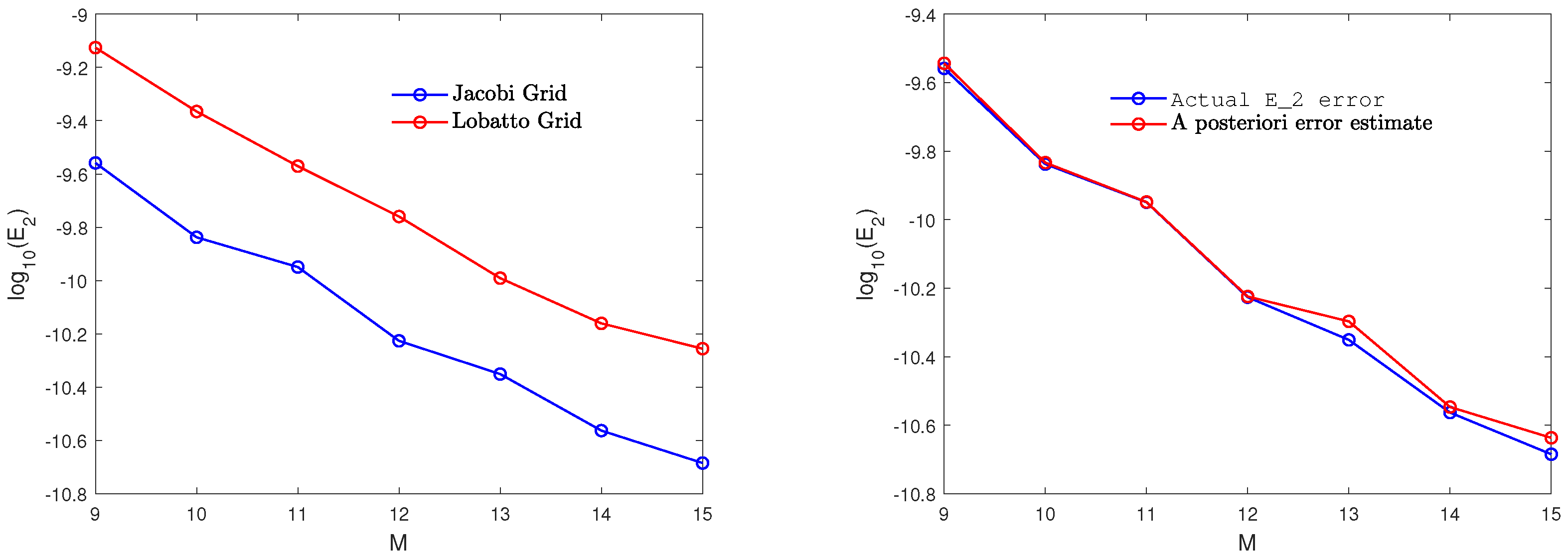
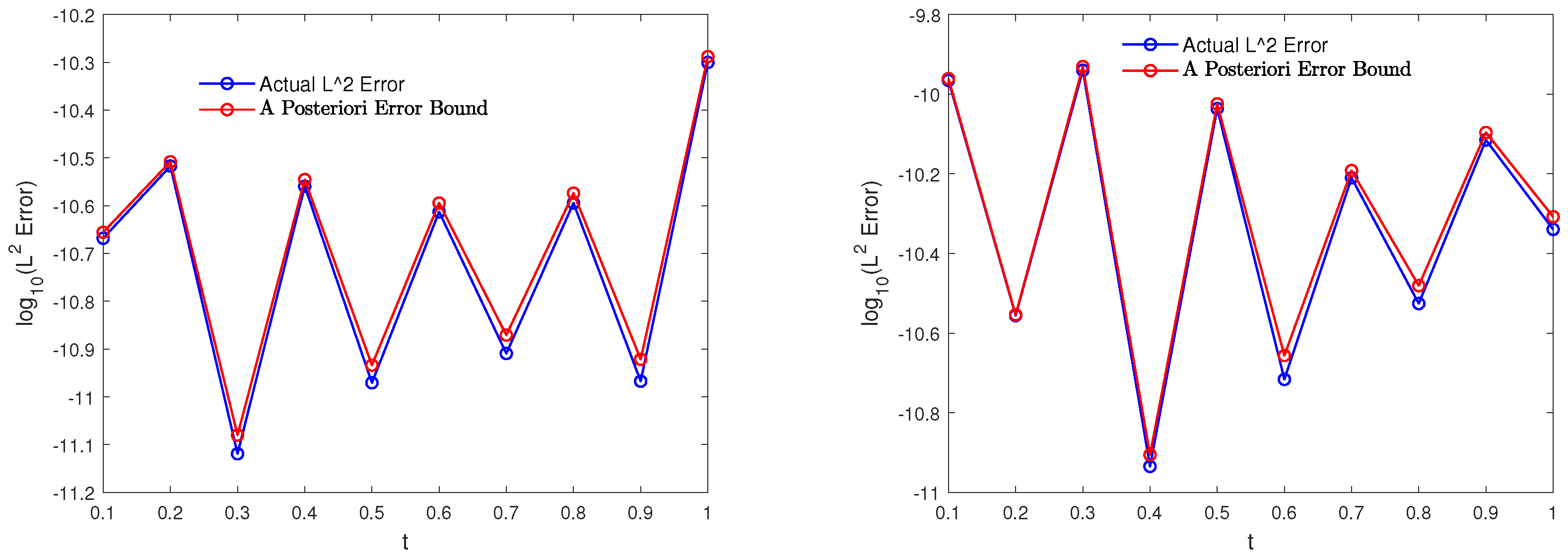
To explicitly quantify the observed convergence rate, we refer to the semi-logarithmic error profiles in Figure 1 (left). In a spectral framework, exponential convergence takes the form $O\left(e^{-cM}\right)$, which mathematically manifests as a strictly linear decrease when plotting ${log}_{10}\left(E\right)$ against the polynomial degree M. The plotted results display this persistent linear decay, visually quantifying the exponential error reduction and confirming that the method achieves true spectral accuracy for this smooth profile, in perfect alignment with the a priori estimates in Theorem 1. Furthermore, the right panel of Figure 1 and the time-evolution plots in Figure 2 quantitatively support the proposed error estimator. By plotting both the actual $E_2$ error and the a posteriori bound, the tightly preserved parallel gap between the curves visually confirms the Effectivity Index. Because the bound strictly upper-bounds the actual error, the condition $EI\ge 1$ is satisfied across all time steps, validating the estimator’s reliability and low variance without the need for additional tabular data. Finally, Figure 2 shows that the error estimator accurately captures localized variations across discrete time steps at higher resolutions, reinforcing the solver’s overall stability and mathematical soundness.

Example 2.

To illustrate the performance of the proposed method, we consider the following fractional partial differential equation:

$${\displaystyle \frac{\mathsf{\partial }w(\xi ,\tau )}{\mathsf{\partial }\tau }}={}_0\mathcal{D}_{\tau }^{1-\alpha }\left[{\displaystyle \frac{{\mathsf{\partial }}^{2}w(\xi ,\tau )}{\mathsf{\partial }{\xi }^2}}-w(\xi ,\tau )\right]+q(\xi ,\tau ),(\xi ,\tau )\in [0,1]\times (0,1].$$

(58)

with homogeneous Dirichlet boundaries

$$w(0,\tau )=0,w(1,\tau )=0,\tau \in [0,1],$$

and the initial condition

$$w(\xi ,0)=0,\xi \in [0,1].$$

Here, the analytical continuous source term $q(\xi ,\tau )$ is defined as

$$q(\xi ,\tau )=(\alpha +2)t^{\alpha +1}{\xi }^2{(1-\xi )}^2+{\displaystyle \frac{\Gamma (3+\alpha )}{2+2\alpha }}{\tau }^{1+2\alpha }({\xi }^4-2{\xi }^3-11{\xi }^2+12\xi -2).$$

(59)

This subdiffusion problem admits the following exact solution [42]:

$$w(\xi ,\tau )={\xi }^2{(1-\xi )}^2{\tau }^{\alpha +2}.$$

(60)

To further validate our Legendre cardinal Galerkin framework, we conducted additional numerical investigations using Example 2. As outlined in

Table 3. The maximum absolute errors ($E_{\infty }$) evaluated with different M values for Example 2.

	Gauss Grid			Lobatto Grid
$\mathit{\tau }\setminus \mathit{M}$	9	13	15	9	13	15
$0.1$	8.34 × 10−8	5.46 × 10−9	3.28 × 10−9	5.22 × 10−7	8.77 × 10−8	1.41 × 10−8
$0.2$	3.38 × 10−8	5.13 × 10−9	5.37 × 10−10	7.12 × 10−7	7.60 × 10−8	3.55 × 10−8
$0.3$	2.87 × 10−8	4.47 × 10−9	8.46 × 10−10	4.36 × 10−7	7.13 × 10−8	4.12 × 10−8
$0.4$	4.80 × 10−8	3.02 × 10−9	1.02 × 10−9	5.59 × 10−7	8.87 × 10−8	3.06 × 10−8
$0.5$	1.29 × 10−8	2.00 × 10−9	7.48 × 10−10	4.68 × 10−7	5.44 × 10−8	2.87 × 10−8
$0.6$	3.27 × 10−8	6.01 × 10−10	7.78 × 10−10	3.39 × 10−7	1.95 × 10−8	1.62 × 10−8
$0.7$	3.28 × 10−8	5.13 × 10−10	7.48 × 10−10	5.82 × 10−7	2.85 × 10−8	1.56 × 10−8
$0.8$	9.78 × 10−9	9.15 × 10−10	1.21 × 10−9	8.09 × 10−8	3.56 × 10−8	1.46 × 10−8
$0.9$	1.62 × 10−8	1.46 × 10−9	1.18 × 10−9	3.95 × 10−7	2.35 × 10−8	2.76 × 10−8
$1.0$	1.38 × 10−7	1.52 × 10−8	6.42 × 10−9	2.27 × 10−7	1.66 × 10−8	5.87 × 10−9
CPU time	$0.610$	$4.812$	$11.219$	$0.641$	$4.312$	$10.531$

, the maximum absolute errors across spatial and temporal resolutions demonstrate consistent high-order accuracy and stable computational performance for both the Jacobi and Lobatto grid configurations. To rigorously assess this efficiency,

Table 4. Comparison of total degrees of freedom (DOFs), the $E_{\infty }$ and $E_2$ errors for Example 2 with existing Compact difference methods [42], taking $\alpha =0.8$.

Method	Total DOFs	${\mathit{E}}_{\mathit{\infty }}$ Error	${\mathit{E}}_2$ Error
Difference method with $h=1/1000,\tau =1/20$	≈20,000	2.45 × 10−4	1.70 × 10−4
Difference method with $h=1/1000,\tau =1/40$	≈40,000	1.08 × 10−4	7.51 × 10−5
Difference method with $h=1/1000,\tau =1/80$	≈80,000	4.73 × 10−5	3.29 × 10−5
Presented Method with Gauss grid ($M=10$)	121	7.24 × 10−8	1.77 × 10−8
Presented Method with Lobatto grid ($M=10$)	121	4.24 × 10−7	1.44 × 10−7

provides a direct comparison with the compact finite-difference approach [42] using the exact same test problem and parameter settings ($\alpha =0.8$). While the finite-difference scheme achieves only an algebraic convergence rate—requiring a massive computational complexity of approximately 80,000 DOFs to reach an error of $O\left({10}^{-5}\right)$—the proposed spectral method achieves $O\left({10}^{-8}\right)$ accuracy with merely 121 DOFs. Supported by the low CPU times documented in Table 3, this stark contrast confirms that the Legendre cardinal framework entirely circumvents the severe computational complexity of dense grid-based solvers.

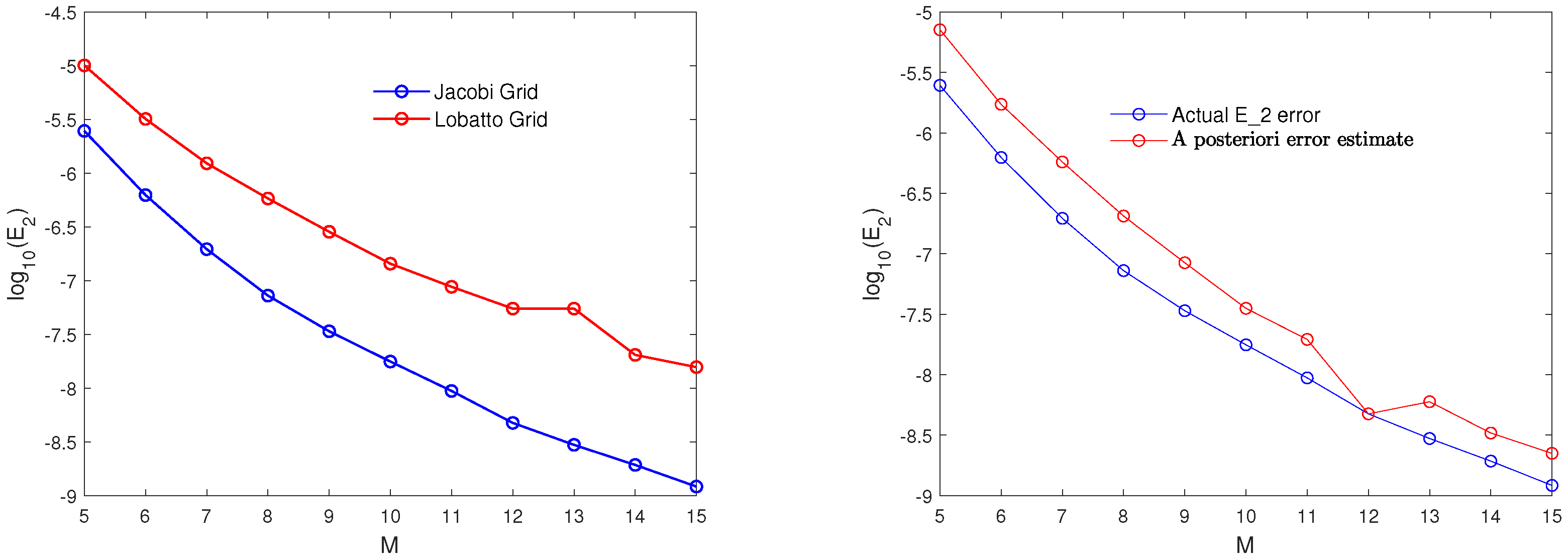
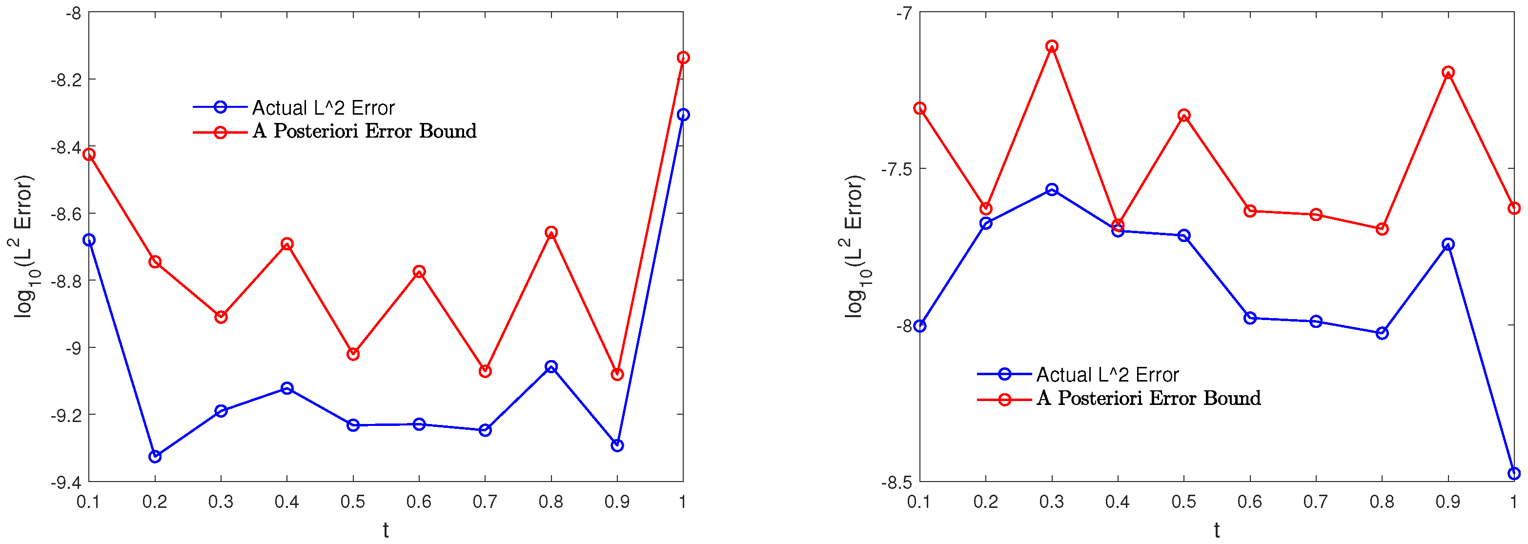
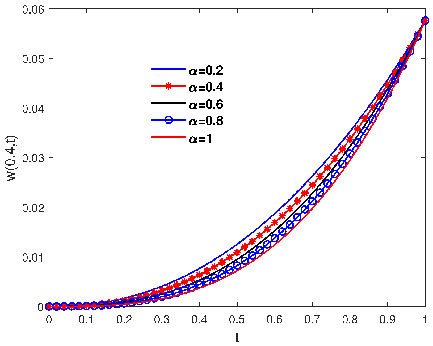
Furthermore, the semi-logarithmic plots in Figure 3 (left) explicitly quantify this convergence behavior. The persistent linear decrease in ${log}_{10}\left(E_2\right)$ as M increases visually confirms the theoretical $O\left(e^{-cM}\right)$ spectral convergence rate, definitively distinguishing this framework from standard methods that yield only algebraic polynomial decay. Alongside this, the right panel of Figure 3 and the detailed temporal profiles in Figure 4 explicitly demonstrate the reliability of our a posteriori bound. The tightly preserved parallel alignment of the actual error and the residual bound across both Gauss and Lobatto grids confirms a highly stable Effectivity Index ($EI\ge 1$), proving that the computable residual serves as a tight, practical proxy for the true error. Finally, the physical impact of memory effects is clearly illustrated in Figure 5, which depicts the solution profiles of $w(0.4,\tau )$ across a spectrum of fractional orders ($\alpha =0.2,0.4,0.6,0.8,1$). As the fractional parameter $\alpha$ increases toward 1, the subdiffusive solution smoothly converges to the classical integer-order limit, visually confirming both the physical consistency and the mathematical stability of the proposed framework. Furthermore, because the temporal discretization uses exact analytical integration via the smooth Gamma function, the system encounters no mathematical singularities or stiffness as $\alpha \to 0^{+}$ or $\alpha \to 1^{-}$. Consequently, the framework fully preserves its high-order spectral accuracy, stable matrix conditioning, and fixed computational runtime across the entire fractional domain without deterioration.

To summarize the computational efficiency demonstrated across both examples, we evaluate the CPU time, system size (total degrees of freedom), and the 2-norm condition number, $\kappa \left(\mathcal{A}\right)$, of the global algebraic systems. As reported in Table 1 and Table 3, the CPU times for assembling and solving these equations remain strictly in the order of seconds. Furthermore, for any chosen resolution M, the total degrees of freedom scale purely as ${(M+1)}^2$. Because the Legendre cardinal framework converges exponentially, exceptional accuracy is achieved with very small polynomial degrees ($M\le 15$), so the maximum global system size in our experiments never exceeds $256\times 256$. Although the condition number $\kappa \left(\mathcal{A}\right)$ of spectral collocation matrices inherently grows with M, these extremely small system sizes ensure that it remains well within the safe operational limits of standard 64-bit double-precision arithmetic (typically $\kappa <{10}^7$). This confirms that the proposed method achieves high accuracy without triggering the massive memory bottlenecks or severe ill-conditioning typical of dense grid-based solvers.

6. Conclusions

In this paper, we introduce a faster and more simple method for solving one-dimensional time-fractional reaction–subdiffusion equations. One of the main challenges in these simulations is addressing early-time singularities and complex numerical integrations, which can significantly slow down the process. We tackled this issue by transforming the original equation into a Volterra integral form, which effectively incorporates the initial conditions and smooths out early spikes. Furthermore, we utilized Legendre cardinal functions, taking advantage of their unique properties related to their nodes. This approach allowed us to construct our matrices directly, thus eliminating the time-consuming process of numerical integration.

Our test results support the theory with strong numerical evidence. The method demonstrated clear exponential convergence, with the error decreasing at a rate of $O\left(e^{-cM}\right)$. In practice, we achieved highly accurate results, with maximum errors around $O\left({10}^{-8}\right)$, using a very small system size of only 100 to 121 points ($M\le 10$). Because the system remains compact, it only takes a few seconds to run, making it significantly faster than standard methods that rely on large space-time grids. Additionally, we confirmed that our error-checking tool operates reliably, maintaining an Effectivity Index (EI) of $EI\ge 1$ throughout the entire process.

Finally, as we adjusted the fractional power $\alpha$, the model smoothly transitioned back to standard diffusion as $\alpha$ approached 1. While the proposed framework demonstrates significant computational advantages, it is important to acknowledge its current limitations. Presently, we have exclusively tested and validated this method for one-dimensional linear problems. Furthermore, because spectral collocation techniques inherently generate dense operational matrices, scaling the method to very high resolutions or multi-dimensional domains will inevitably increase memory requirements and computational overhead. However, since this approach successfully avoids extensive numerical integration and maintains exceptionally small matrix sizes for smooth problems, we believe it provides a solid, practical foundation. Future work will focus on extending this methodology to multidimensional and nonlinear fractional equations, potentially coupling it with sparse iterative solvers to manage the dense matrix constraints.

References

1. Diethelm, K. The Analysis of Fractional Differential Equations; Springer: Berlin/Heidelberg, Germany, 2010. [Google Scholar]
2. Mainardi, F. Fractional Calculus and Waves in Linear Viscoelasticity; Imperial College Press: London, UK, 2010. [Google Scholar]
3. Luchko, Y. Anomalous diffusion models and their analysis. Fract. Calc. Appl. Anal. 2012, 15, 141–146. [Google Scholar] [CrossRef] [Scilit]
4. Podlubny, I. Fractional Differential Equations; Academic Press: San Diego, CA, USA, 1999. [Google Scholar]
5. Kilbas, A.A.; Srivastava, H.M.; Trujillo, J.J. Theory and Applications of Fractional Differential Equations; Elsevier B.V.: Amsterdam, The Netherlands, 2006. [Google Scholar]
6. Gorenflo, R.; Mainardi, F.; Moretti, D.; Pagnini, G.; Paradisi, P. Discrete random walk models for space-time fractional diffusion. Chem. Phys. 2002, 284, 521–541. [Google Scholar] [CrossRef] [Scilit]
7. Metzler, R.; Klafter, J. The random walk’s guide to anomalous diffusion: A fractional dynamics approach. Phys. Rep. 2000, 339, 1–77. [Google Scholar] [CrossRef] [Scilit]
8. Henry, B.I.; Wearne, S.L. Fractional reaction-diffusion. Phys. A Stat. Mech. Its Appl. 2000, 276, 448–455. [Google Scholar] [CrossRef] [Scilit]
9. Langlands, T.A.M.; Henry, B.I.; Wearne, S.L. Anomalous subdiffusion with multispecies linear reaction dynamics. Phys. Rev. E Stat. Nonlinear Soft Matter Phys. 2008, 77, 021111. [Google Scholar] [CrossRef] [Scilit] [PubMed]
10. Yuste, S.B. Weighted average finite difference methods for fractional diffusion equations. J. Comput. Phys. 2006, 216, 264–274. [Google Scholar] [CrossRef] [Scilit]
11. Murio, D.A. Implicit finite difference approximation for time fractional diffusion equations. Comput. Math. Appl. 2008, 56, 1138–1145. [Google Scholar] [CrossRef] [Scilit]
12. Sun, Z.; Wu, X. A fully discrete difference scheme for a diffusion-wave system. Appl. Numer. Math. 2006, 56, 193–209. [Google Scholar] [CrossRef] [Scilit]
13. Cui, M. Compact finite difference method for the fractional diffusion equation. J. Comput. Phys. 2009, 228, 7792–8004. [Google Scholar] [CrossRef] [Scilit]
14. Zhuang, P.; Liu, F.; Anh, V.; Turner, I. New solution and analytical techniques of the implicit numerical method for the anomalous subdiffusion equation. SIAM J. Numer. Anal. 2008, 46, 1079–1095. [Google Scholar] [CrossRef] [Scilit]
15. Maji, S.; Natesan, S. Adaptive-grid technique for the numerical solution of a class of fractional boundary-value-problems. Comput. Methods Differ. Equ. 2010, 12, 338–349. [Google Scholar]
16. Kammappa, Z.; Awasthi, A. Trigonometric cubic B-spline collocation method for time fractional diffusion equation. Comput. Methods Differ. Equ. 2025, in press. [Google Scholar] [CrossRef] [Scilit]
17. Ebrahimi, M.; Matinfar, M.; Babaei, A. Numerical solution for an inverse source problem of a fractional order diffusion-wave equation. Comput. Methods Differ. Equ. 2025, in press. [Google Scholar] [CrossRef] [Scilit]
18. Radmanesh, M.; Ebadi, M.J. A local mesh-less collocation method for solving a class of time-dependent fractional integral equations: 2D fractional evolution equation. Eng. Anal. Bound. Elem. 2020, 113, 372–381. [Google Scholar] [CrossRef] [Scilit]
19. Abdollahi, Z.; Moghadam, M.M.; Saeedi, H.; Ebadi, M.J. A computational approach for solving fractional Volterra integral equations based on two-dimensional Haar wavelet method. Int. J. Comput. Math. 2022, 99, 1488–1504. [Google Scholar] [CrossRef] [Scilit]
20. Zeeshan Ali, K.; Mahariq, I.; Ebadi, M.J. A hybrid Laplace-spectral method for time-fractional wave equations: Numerical modelling. Int. J. Numer. Model. 2025, 38, e70129. [Google Scholar] [CrossRef] [Scilit]
21. Hong, A.; Liao, X.; Hui, H. Simulation of soil collapse based on the local radial basis function collocation method. Eng. Anal. Bound. Elem. 2026, 186, 106687. [Google Scholar] [CrossRef] [Scilit]
22. Li, X.; Tian, H.; Zhang, P.; Liu, X. Existence, Uniqueness, and Continuous Dependence on Initial/Final Values for Liouville–Caputo Fractional Difference Equations. Fractal Fract. 2026, 10, 504. [Google Scholar] [CrossRef] [Scilit]
23. Chen, S.; Liu, F.; Turner, I.; Anh, V. A Fourier method for the fractional diffusion equation describing sub-diffusion. J. Comput. Phys. 2007, 227, 886–897. [Google Scholar] [CrossRef] [Scilit]
24. Dimitrov, Y.; Georgiev, S.; Todorov, V. Approximation of Caputo Fractional Derivative and Numerical Solutions of Fractional Differential Equations. Fractal Fract. 2023, 7, 750. [Google Scholar] [CrossRef] [Scilit]
25. Jin, B.; Lazarov, R.; Zhou, Z. Error estimates for a semidiscrete finite element method for fractional order parabolic equations. SIAM J. Numer. Anal. 2013, 51, 445–466. [Google Scholar] [CrossRef] [Scilit]
26. Zeng, F.; Li, C.; Liu, F.; Turner, I. The use of finite difference/element approaches for solving the time-fractional subdiffusion equation. SIAM J. Sci. Comput. 2013, 35, A2976–A3000. [Google Scholar] [CrossRef] [Scilit]
27. Salama, F.M.; Balasim, A.T.; Ali, U.; Khan, M.A. Efficient numerical simulations based on an explicit group approach for the time fractional advection-diffusion reaction equation. Comput. Appl. Math. 2023, 42, 168. [Google Scholar] [CrossRef] [Scilit]
28. Abbaszadeh, M.; Dehghan, M. A meshless numerical procedure for solving fractional reaction subdiffusion model via a new combination of alternating direction implicit (ADI) approach and interpolating element free Galerkin (EFG) method. Comput. Math. Appl. 2015, 70, 2493–2512. [Google Scholar] [CrossRef] [Scilit]
29. Adeoye, A.S.; Omole, E.O.; Omolofe, B.; Fayose, T.S.; Smerat, A. A Numerov–Galerkin Framework for the Transient Dynamics of Anisotropic Plates on Vlasov Foundations. Algorithms 2026, 19, 578. [Google Scholar] [CrossRef] [Scilit]
30. Li, X.; Xu, C. A space-time spectral method for the time fractional diffusion equation. SIAM J. Numer. Anal. 2009, 47, 2108–2131. [Google Scholar] [CrossRef] [Scilit]
31. Shen, J.; Tang, T.; Wang, L.L. Spectral Methods: Algorithms, Analysis, Applications; Springer: Berlin/Heidelberg, Germany, 2011. [Google Scholar]
32. Zayernouri, M.; Karniadakis, G.E. Fractional spectral collocation method. SIAM J. Sci. Comput. 2013, 36, A40–A62. [Google Scholar] [CrossRef] [Scilit]
33. Afarideh, A.; Dastmalchi Saei, F.; Lakestani, M.; Saray, B.N. Pseudospectral method for solving fractional Sturm-Liouville problem using Chebyshev cardinal functions. Phys. Scr. 2021, 96, 125267. [Google Scholar] [CrossRef] [Scilit]
34. Afarideh, A.; Dastmalchi Saei, F.; Saray, B.N. Eigenvalue problem with fractional differential operator: Chebyshev cardinal spectral method. J. Math. Model. 2021, 11, 343–355. [Google Scholar]
35. Asadzadeh, M.; Saray, B.N. On a multiwavelet spectral element method for integral equation of a generalized Cauchy problem. BIT Numer. Math. 2022, 62, 383–416. [Google Scholar] [CrossRef] [Scilit]
36. Shi, L.; Saray, B.N.; Soleymani, F. Sparse wavelet Galerkin method: Application for fractional Pantograph problem. J. Comput. Appl. Math. 2024, 451, 116081. [Google Scholar] [CrossRef] [Scilit]
37. Hadi, M.S.; Lakestani, M.; Saray, B.N. The wavelet Galerkin method for fractional delay differential equations. Calcolo 2025, 62, 48. [Google Scholar] [CrossRef] [Scilit]
38. Shahriari, M.; Saray, B.N.; Mohammadalipour, B.; Saeidian, S. Pseudospectral method for solving the fractional one-dimensional Dirac operator using Chebyshev cardinal functions. Phys. Scr. 2023, 98, 055205. [Google Scholar] [CrossRef] [Scilit]
39. Liu, T.; Ding, B.; Saray, B.N.; Juraev, D.A.; Elsayed, E.E. On the pseudospectral method for solving the fractional Klein-Gordon equation using Legendre cardinal functions. Fractal Fract. 2025, 9, 177. [Google Scholar] [CrossRef] [Scilit]
40. Mahshidnia, M.; Mahmoudi, Y.; Saray, B.N.; Rad, M.J. A novel collocation method for fractional delay differential equations with Legendre cardinal functions. Phys. Scr. 2026, 101, 015207. [Google Scholar] [CrossRef] [Scilit]
41. Dehghan, M.; Abbaszadeh, M.; Mohebbi, A. Error estimate for the numerical solution of fractional reaction-subdiffusion process based on a meshless method. J. Comput. Appl. Math. 2015, 280, 14–36. [Google Scholar] [CrossRef] [Scilit]
42. Cao, J.; Li, C.; Chen, Y. Compact difference method for solving the fractional reaction-subdiffusion equation with Neumann boundary value condition. Int. J. Comput. Math. 2015, 92, 167–180. [Google Scholar] [CrossRef] [Scilit]
Figure 1. Evolution of the actual L 2 error demonstrating the strictly linear (exponential) spectral convergence rate for different choices of grid (left), and a comparison between the actual E 2 error and the a posteriori error bound explicitly verifying the Effectivity Index E I 1 (right), for Example 1.
Mathematics 14 03183 g001
Figure 2. Evolution of the actual L 2 error and the a posteriori error bound over continuous time τ , taking M = 15 . Results using the Legendre–Gauss grid (left) and Legendre–Gauss–Lobatto grid (right) for Example 1, confirming the stability of the error estimator and the tight Effectivity Index across discrete time steps.
Mathematics 14 03183 g002
Figure 3. Evolution of the actual L 2 error quantifying the spectral convergence rate for different choices of grid (left), and a direct comparison between the actual E 2 error and the a posteriori error bound visually demonstrating the Effectivity Index (right), for Example 2.
Mathematics 14 03183 g003
Figure 4. Evolution of the actual L 2 error and the a posteriori error bound over time τ , taking M = 15 . Results using the Legendre–Gauss grid (left) and Legendre–Gauss–Lobatto grid (right) for Example 2, confirming that the residual acts as a reliable proxy for the true error.
Mathematics 14 03183 g004
Figure 5. Behavior of the numerical solution w ( 0.4 , τ ) for Example 2 under various fractional orders α . The plot explicitly demonstrates the smooth physical transition from fractional subdiffusive memory dynamics ( α < 1 ) to the classical integer-order diffusion limit ( α = 1 ).
Mathematics 14 03183 g005