A Residual-Adaptive Preconditioned ψ-Fractional Quantum Pseudo-Spectral Method: Delay-Memory Differential Equations

Abstract

We develop a residual-adaptive preconditioned quantum pseudo-spectral method for generalised $\psi$-Caputo initial-value problems containing a discrete delay, weakly singular hereditary memory, and nonlinear reaction terms. A $\psi$-fractional Chebyshev basis yields closed-form operational matrices that are exact on the chosen finite spectral space. To make the hereditary term compatible with block encoding, the power-law kernel is approximated by a sum of exponentials and supplemented by an explicit local near-field correction, converting global memory into finitely many local auxiliary modes. A structure-preserving preconditioner controls the condition number, while a residual-adaptive multidomain strategy and damped Newton iteration treat layers and nonlinearities. We prove well-posedness in Mittag–Leffler weighted graph spaces, derive a combined spectral–kernel–residual error estimate, and state the quantum linear-system complexity with explicit block-encoding normalisations and right-hand-side preparation assumptions. Numerical tests show high accuracy for solutions smooth in the $\psi$-coordinate, improved robustness for singular and layered solutions, substantial condition-number reduction, and lower history cost under sum-of-exponentials compression. To evaluate performance, we compare against L1 product integration and Jacobi collocation, systematically quantifying their respective accuracy, computational cost, and conditioning characteristics.

1. Introduction

Fractional differential equations have become a standard modelling language whenever a process retains a long memory of its own history, because the fractional derivative encodes nonlocality in time through a weakly singular convolution against the unknown [1,2,3]. The classical Riemann–Liouville and Caputo operators have since been unified and considerably generalised by Almeida’s Caputo derivative of a function with respect to a kernel $\psi$, the $\psi$-Caputo derivative, which recovers the Caputo, Caputo–Hadamard, and Erdélyi–Kober families as special choices of the kernel and provides a single tunable clock against which memory is measured [4,5]. The analytic theory of $\psi$-fractional problems is now well developed, including qualitative studies of relaxation and oscillation [6], systems of $\psi$-Caputo equations [7], functional equations [8], the $\psi$-Hilfer calculus and its Gronwall inequalities [9], weighted generalizations [10], and recent applications to stochastic finance [11] and evolution systems of order between one and two. The Mittag–Leffler function and its generalisations sit at the centre of this theory, both as the spectral object that governs fractional relaxation and as the natural weight in fixed-point arguments [12,13].

Three numerical strands are directly relevant to the present problem. First, spectral and pseudo-spectral collocation methods are attractive for fractional delay and Volterra equations because they can attain high-order or spectral convergence when the solution is sufficiently regular in the appropriate transformed coordinate. Fractional pantograph and delay equations have been treated using rescaled and mapped bases [14] and functional collocation frameworks [15]. Related spectral-element formulations based on Jacobi polyfractonomials and Jacobi spectral-collocation methods for Volterra equations with weakly singular kernels provide complementary convergence analyses [16,17]. These approaches accurately resolve delay or Volterra nonlocality, but the resulting hereditary operators are generally dense, and their conditioning and algebraic structure are not designed for implementation through a quantum linear-system solver.

Second, classical fast-memory algorithms approximate a weakly singular power-law kernel by a sum of exponentials. The construction introduced by Jiang et al. [18], together with the fast and oblivious convolution framework, exponential-sum approximation theory, and related kernel-compression procedures [19,20,21], replaces repeated global convolution, for a prescribed kernel tolerance, by a fixed collection of local recurrence relations. This localisation substantially reduces the storage and sequential history costs. Nevertheless, these methods are primarily classical time-stepping or kernel-compression procedures and do not, by themselves, provide a general $\psi$-fractional spectral basis, an exact delay operational matrix, a quantum-oriented preconditioner, a residual-adaptive multidomain strategy, or a block-encoding analysis.

Third, quantum algorithms for differential equations have developed from the Harrow–Hassidim–Lloyd quantum linear-system algorithm [22] to increasingly sophisticated solvers for linear and nonlinear differential equations [23,24,25,26,27]. Quantum spectral methods, in which a high-order discretisation is encoded and inverted on a quantum register, were subsequently analyzed by Childs and Liu [28]. The associated algorithmic framework now includes quantum singular-value transformation [29], optimal and near-optimal quantum linear-system solvers [30,31,32], eigenstate filtering and quantum eigenvalue processing [33,34], time-marching and Dyson-series solvers [35,36], Lindbladian and Schrodingerisation formulations [37,38], Pad’e-based autonomous solvers [39], explicit block encodings for boundary-value operators [40], practical quantum resource estimates [41], adiabatic-inspired linear-system algorithms [42], improved higher-order nonlinear differential-equation solvers [43], and hybrid quantum–classical spectral methods [44]. Across these developments, the relevant computational resources are not determined solely by the algebraic dimension. They also depend on the sparsity and block-encoding normalisation of the operator, its condition number, the cost of preparing the right-hand side, and the measurements required to extract useful information from the quantum solution state. A direct discretisation of a weakly singular hereditary term is therefore problematic because its history coupling grows with the spectral order and destroys the locality required for an efficient block encoding.

The principal point of departure for the present work is the quantum pseudo-spectral construction of Abbasbandy [45]. That method employs a fractional shifted-Chebyshev basis for single-term Caputo equations, avoids the need for a fractional chain rule in the treatment of nonlinear terms, and produces a triangular operational derivative matrix with a structured representation suitable for a quantum linear-system algorithm. A related hybrid quantum-spectral-successive-linearisation treatment of Lane–Emden-type equations was developed in [46]. These methods, however, do not simultaneously accommodate a general $\psi$-clock, a discrete time delay, a weakly singular hereditary memory term, local history compression, residual-adaptive multidomain refinement, and a computable condition-number certificate. These omissions are structural: directly appending hereditary memory produces a dense global-history block, whereas delay terms and multidomain interface constraints introduce additional nonlocal couplings.

The present method closes these gaps by combining exact-on-space $\psi$-fractional operational matrices with an explicit delay matrix, a local-plus-near-field sum-of-exponentials representation of the hereditary kernel, a structure-preserving preconditioner, and a classical residual-adaptive outer loop whose fixed-partition algebraic operator is block encodable.

The principal distinctions among the three relevant numerical strands and the proposed RAP-QPSM framework are summarised in

Table 1. Position of the present method relative to the principal numerical strands.

Framework	Model Scope	History and Conditioning	Computational Realisation
Fractional delay spectral methods [16]	Classical clock; discrete delay; fractional dynamics	Dense or problem-dependent history; basis-dependent conditioning	Classical spectral or spectral-element solve
Jacobi Volterra collocation [17]	Weakly singular Volterra memory; delay optional	Dense memory collocation; no quantum-oriented preconditioner	Classical dense collocation
Fast SOE convolution [18,20]	Usually identity-clock fractional memory; delay optional	Local recurrences; reduced sequential history cost	Fast classical time stepping
Quantum pseudo-spectral method [45]	Single-term Caputo equations; no delay or hereditary memory	Structured derivative block; no memory localisation required	Global quantum spectral solve
Present RAP-QPSM	General $\psi$-clock; discrete delay; weakly singular memory	SOE plus near-field correction; computable preconditioning certificate	Residual-adaptive outer loop and fixed-partition block encoding

.

To quantify the specific computational advantage obtained by localising the hereditary term,

Table 2. Structural cost of the hereditary term for $N+1$ temporal degrees of freedom. The spectral derivative blocks remain structured dense blocks; the table isolates the additional history coupling.

Memory Representation	Stored History Data	Per-Row History Coupling	Sequential History Work
Direct collocation matrix $\mathbb{M}$	$O\left(N^2\right)$ entries	$O\left(N\right)$	$O\left(N^2\right)$ total
Direct L1/product integration	$O\left(N\right)$ states	$O\left(N\right)$ at step n	$O\left(N^2\right)$ total
SOE augmentation with fixed Q	$O\left(QN\right)$ augmented values or $O\left(Q\right)$ sequential modes	$O\left(Q\right)$ local diagonals	$O\left(QN\right)$ total

compares the storage, per-row coupling, and sequential history costs of direct collocation, product-integration, and SOE-augmented formulations.

The SOE reformulation does not make the spectral differentiation matrices elementwise sparse. Its precise benefit is to remove the N-growing hereditary coupling and replace it by Q local modes; the preconditioner separately controls the condition number. The specific contributions are the following.

1.

A generalised $\psi$-fractional delay–memory model (Section 3) with global well-posedness in a Mittag–Leffler weighted graph space for the multi-term equation and a Carathéodory local theory for bounded measurable coefficients, locally Lipschitz nonlinearities, and $L^p$ forcing.

2.

A $\psi$-fractional Chebyshev basis whose generalised Vandermonde, $\psi$-Caputo, delay, and memory operational matrices are obtained in closed form. Exactness is stated precisely on the represented finite spectral space, with the general consistency error identified as the fractional derivative of the interpolation error.

3.

A sum-of-exponentials compression of the weakly singular $\psi$-kernel together with an explicit polynomial near-field correction and a unified local-plus-history error estimate. The resulting augmented system replaces the dense hereditary block by Q local modes.

4.

A block encoding of the preconditioned augmented operator and a solution-state complexity theorem that records the product normalisation, right-hand-side preparation probability, preconditioned condition number, and augmented dimension.

5.

A structure-preserving preconditioner with both an abstract condition-number bound and a computable pre-solve certificate, together with a propagation estimate along the nonlinear Newton iteration.

6.

A residual-adaptive multidomain algorithm whose patch selection is a classical outer loop; for a fixed partition, local operators, sparse interface rows, and transferred memory modes admit a patch-selected block encoding.

7.

Six model studies and a separate four-method benchmark comparing RAP-QPSM with Jacobi collocation, L1 product integration, and SOE-accelerated L1 history in accuracy, measured computational cost, and conditioning.

Throughout, $\psi$ is a strictly increasing $C^1$ kernel on the working interval and the time variable is denoted $\xi$. The symbols used in the paper are collected in Table 3.

The remainder of the paper is organised as follows. Section 2 recalls the required $\psi$-fractional calculus, Mittag–Leffler weighted spaces, and memory bounds. Section 3 formulates the delay–memory problem and proves well-posedness, including the variable-coefficient multi-term case in a graph space and a local Carathéodory extension. Section 4 constructs the $\psi$-fractional Chebyshev basis and the operational matrices, whose exactness is stated on the represented finite spectral space. Section 5 develops SOE compression together with the local near-field correction and its unified residual contribution. Section 6 gives the fixed-partition block encoding, explicit normalisation-dependent QLSA complexity, logical-resource proxies, and the multidomain stitching construction. Section 7 establishes the condition-number bound and a computable pre-solve certificate propagated through Newton updates. Section 8 presents the residual-adaptive multidomain and damped-Newton algorithms, while Section 9 reports the six model studies and quantitative comparisons with Jacobi collocation, L1 product integration, and SOE–L1 history compression. Section 10 and Section 11 discuss the principal findings and summarise their significance.

Table 3. Principal notation.

Symbol	Description
Clock, coordinate, and exponents
$\xi$	time variable
$\psi$	strictly increasing $C^1$ kernel (memory clock)
$[a,b]$	working interval; ${\mathsf{\Psi }}_{♭}=\psi \left(b\right)-\psi \left(a\right)$ total clock increment
$\vartheta$	normalised coordinate $\vartheta =(\psi \left(\xi \right)-\psi \left(a\right))/{\mathsf{\Psi }}_{♭}\in [0,1]$
$\eta \left(\xi \right)$	clock increment $\eta \left(\xi \right)=\psi \left(\xi \right)-\psi \left(a\right)$
$\alpha ,\beta$	fractional orders, $0<\beta <\alpha <1$
$\nu$	singularity exponent of the memory kernel, $0<\nu <1$
q	fractional basis exponent
$\epsilon$	singular-perturbation scale, $0<\epsilon \le 1$
$\tau$	time delay; $\phi$ history function on $[a-\tau ,a]$
Operators
${{}^{\mathcal{C}}\mathfrak{D}}^{\mu ;\psi }$	$\psi$-Caputo derivative of order $\mu$
${\mathcal{I}}^{\mu ;\psi }$	$\psi$-fractional (Riemann–Liouville) integral of order $\mu$
${\mathcal{M}}_{\psi ,\nu }$	weakly singular $\psi$-memory operator (kernel K, exponent $\nu$)
$L,\mathcal{L}$	continuous and discrete (collocation) operators
$\mathcal{P}$	structure-preserving preconditioner
Solution and basis
$u,u_N$	exact solution and degree-N spectral solution
${\mathsf{B}}_n$	$\psi$-fractional Chebyshev basis function
${\chi }_i$	collocation nodes (${\chi }_0=b,{\chi }_N=a$)
$\phi$	history function on $[a-\tau ,a]$
$g,F$	forcing term and Lipschitz nonlinearity
${\mathrm{\Pi }}_N$	interpolation onto $span{\left\{{\mathsf{B}}_n\right\}}_{n\le N}$
Discrete matrices
$\mathbb{V},{\mathbb{V}}_{\mu },{\mathbb{V}}_{\mathcal{M}}$	generalised Vandermonde, derivative and memory Vandermonde
${\mathbb{D}}^{\left(\mu \right)}$	exact-on-space $\psi$-Caputo operational matrix, ${\mathbb{D}}^{\left(\mu \right)}={\mathbb{V}}_{\mu }{\mathbb{V}}^{-1}$
${\mathbb{H}}_{\tau }$	delay operational matrix
$\mathbb{M}$	weakly singular memory operational matrix
$\mathcal{E}$	perturbation $\mathcal{L}-\mathcal{P}$ in the conditioning bound
Memory compression and quantum step
$w_{\mathsf{\ell }}{e}^{-{\varpi }_{\mathsf{\ell }}t}$	sum-of-exponentials surrogate of $t^{-\nu }$
${\varpi }_{\mathsf{\ell }},w_{\mathsf{\ell }},Q$	SOE rates, weights and number of modes
$m_{\mathsf{\ell }}\left(\xi \right)$	local exponential memory mode
$\tilde{\mathcal{L}},\tilde{\mathit{u}},\tilde{\mathit{g}}$	augmented operator, unknown and right-hand side
${\alpha }_{\tilde{\mathcal{L}}},{\alpha }_{{\mathcal{P}}^{-1}}$	block-encoding normalisations of $\tilde{\mathcal{L}}$ and ${\mathcal{P}}^{-1}$
${\kappa }_{\mathcal{P}}$	bound on ${\kappa }_2\left({\mathcal{P}}^{-1}\tilde{\mathcal{L}}\right)$
${\kappa }_{\mathrm{eff}}$	effective QLSA parameter ${\alpha }_B{∥B^{-1}∥}_2$ for the normalised preconditioned operator
$|\Xi \rangle$	prepared (amplitude-encoded) solution state
Special functions and norms
$E_{\alpha ,\beta },E_{\alpha }$	two- and one-parameter Mittag–Leffler functions
$M_{\alpha ,\mu }$	constant in the mixed-order Mittag–Leffler bound
${∥·∥}_{\infty },{∥·∥}_{*}$	supremum norm and Mittag–Leffler weighted norm
$E_{\infty },{\mathcal{R}}_{\infty }$	error and exact residual in the supremum norm
${\kappa }_L,{\kappa }_P$	condition numbers ${\kappa }_2\left(\mathcal{L}\right)$ and ${\kappa }_2\left({\mathcal{P}}^{-1}\mathcal{L}\right)$

Table 3. Principal notation.

Symbol	Description
Clock, coordinate, and exponents
$\xi$	time variable
$\psi$	strictly increasing $C^1$ kernel (memory clock)
$[a,b]$	working interval; ${\mathsf{\Psi }}_{♭}=\psi \left(b\right)-\psi \left(a\right)$ total clock increment
$\vartheta$	normalised coordinate $\vartheta =(\psi \left(\xi \right)-\psi \left(a\right))/{\mathsf{\Psi }}_{♭}\in [0,1]$
$\eta \left(\xi \right)$	clock increment $\eta \left(\xi \right)=\psi \left(\xi \right)-\psi \left(a\right)$
$\alpha ,\beta$	fractional orders, $0<\beta <\alpha <1$
$\nu$	singularity exponent of the memory kernel, $0<\nu <1$
q	fractional basis exponent
$\epsilon$	singular-perturbation scale, $0<\epsilon \le 1$
$\tau$	time delay; $\phi$ history function on $[a-\tau ,a]$
Operators
${{}^{\mathcal{C}}\mathfrak{D}}^{\mu ;\psi }$	$\psi$-Caputo derivative of order $\mu$
${\mathcal{I}}^{\mu ;\psi }$	$\psi$-fractional (Riemann–Liouville) integral of order $\mu$
${\mathcal{M}}_{\psi ,\nu }$	weakly singular $\psi$-memory operator (kernel K, exponent $\nu$)
$L,\mathcal{L}$	continuous and discrete (collocation) operators
$\mathcal{P}$	structure-preserving preconditioner
Solution and basis
$u,u_N$	exact solution and degree-N spectral solution
${\mathsf{B}}_n$	$\psi$-fractional Chebyshev basis function
${\chi }_i$	collocation nodes (${\chi }_0=b,{\chi }_N=a$)
$\phi$	history function on $[a-\tau ,a]$
$g,F$	forcing term and Lipschitz nonlinearity
${\mathrm{\Pi }}_N$	interpolation onto $span{\left\{{\mathsf{B}}_n\right\}}_{n\le N}$
Discrete matrices
$\mathbb{V},{\mathbb{V}}_{\mu },{\mathbb{V}}_{\mathcal{M}}$	generalised Vandermonde, derivative and memory Vandermonde
${\mathbb{D}}^{\left(\mu \right)}$	exact-on-space $\psi$-Caputo operational matrix, ${\mathbb{D}}^{\left(\mu \right)}={\mathbb{V}}_{\mu }{\mathbb{V}}^{-1}$
${\mathbb{H}}_{\tau }$	delay operational matrix
$\mathbb{M}$	weakly singular memory operational matrix
$\mathcal{E}$	perturbation $\mathcal{L}-\mathcal{P}$ in the conditioning bound
Memory compression and quantum step
$w_{\mathsf{\ell }}{e}^{-{\varpi }_{\mathsf{\ell }}t}$	sum-of-exponentials surrogate of $t^{-\nu }$
${\varpi }_{\mathsf{\ell }},w_{\mathsf{\ell }},Q$	SOE rates, weights and number of modes
$m_{\mathsf{\ell }}\left(\xi \right)$	local exponential memory mode
$\tilde{\mathcal{L}},\tilde{\mathit{u}},\tilde{\mathit{g}}$	augmented operator, unknown and right-hand side
${\alpha }_{\tilde{\mathcal{L}}},{\alpha }_{{\mathcal{P}}^{-1}}$	block-encoding normalisations of $\tilde{\mathcal{L}}$ and ${\mathcal{P}}^{-1}$
${\kappa }_{\mathcal{P}}$	bound on ${\kappa }_2\left({\mathcal{P}}^{-1}\tilde{\mathcal{L}}\right)$
${\kappa }_{\mathrm{eff}}$	effective QLSA parameter ${\alpha }_B{∥B^{-1}∥}_2$ for the normalised preconditioned operator
$|\Xi \rangle$	prepared (amplitude-encoded) solution state
Special functions and norms
$E_{\alpha ,\beta },E_{\alpha }$	two- and one-parameter Mittag–Leffler functions
$M_{\alpha ,\mu }$	constant in the mixed-order Mittag–Leffler bound
${∥·∥}_{\infty },{∥·∥}_{*}$	supremum norm and Mittag–Leffler weighted norm
$E_{\infty },{\mathcal{R}}_{\infty }$	error and exact residual in the supremum norm
${\kappa }_L,{\kappa }_P$	condition numbers ${\kappa }_2\left(\mathcal{L}\right)$ and ${\kappa }_2\left({\mathcal{P}}^{-1}\mathcal{L}\right)$

2. Preliminaries

Let $[a,b]\subset \mathbb{R}$ and let $\psi \in C^1\left([a,b]\right)$ be strictly increasing, so that ${\psi }^{\prime }\left(\xi \right)>0$ and $\psi$ admits a $C^1$ inverse. We write ${\mathsf{\Psi }}_{♭}:=\psi \left(b\right)-\psi \left(a\right)$ and define the normalised coordinate

$$\vartheta \left(\xi \right):={\displaystyle \frac{\psi \left(\xi \right)-\psi \left(a\right)}{{\mathsf{\Psi }}_{♭}}}\in [0,1],\xi \in [a,b].$$

(1)

Definition 1 ($\psi$-fractional integral and $\psi$-Caputo derivative).

For $\mu >0$ and $h\in C\left(\right[a,b\left]\right)$ the ψ-fractional integral is

$${\mathcal{I}}^{\mu ;\psi }h\left(\xi \right)={\displaystyle \frac{1}{\mathrm{\Gamma }\left(\mu \right)}}{\int }_a^{\xi }{\psi }^{\prime }\left(s\right){\left(\psi \left(\xi \right)-\psi \left(s\right)\right)}^{\mu -1}h\left(s\right)\mathrm{d}s,$$

(2)

and for $0<\mu <1$ and $h\in C^1\left([a,b]\right)$, the ψ-Caputo derivative is

$${{}^{\mathcal{C}}\mathfrak{D}}^{\mu ;\psi }h\left(\xi \right)={\displaystyle \frac{1}{\mathrm{\Gamma }(1-\mu )}}{\int }_a^{\xi }{\left(\psi \left(\xi \right)-\psi \left(s\right)\right)}^{-\mu }{h}^{\prime }\left(s\right)\mathrm{d}s={\mathcal{I}}^{1-\mu ;\psi }\left[{\displaystyle \frac{h^{\prime }}{{\psi }^{\prime }}}\right]\left(\xi \right).$$

(3)

The choice $\psi \left(\xi \right)=\xi$ gives the Caputo derivative and $\psi \left(\xi \right)=log\xi$ gives the Caputo–Hadamard derivative [4,5].

The two-parameter Mittag–Leffler function is $E_{\alpha ,\beta }\left(z\right)={\sum }_{k\ge 0}{z}^k/\mathrm{\Gamma }(\alpha k+\beta )$, which is entire and, for $z\ge 0$, strictly positive and strictly increasing; we write $E_{\alpha }:=E_{\alpha ,1}$ [12]. We record the identities on which the operational matrices and the well-posedness proofs rest: the power rule, the Mittag–Leffler self-map of the $\psi$-fractional integral, and a mixed-order generalisation of the latter that is needed for the multi-term equation.

Lemma 1 ($\psi$-power rule).

For $\rho \ge 0$ and $0<\mu <1$,

$${{}^{\mathcal{C}}\mathfrak{D}}^{\mu ;\psi }\left(\vartheta {\left(\xi \right)}^{\rho }\right)={\displaystyle \frac{\mathrm{\Gamma }(\rho +1)}{\mathrm{\Gamma }(\rho -\mu +1)}}{\mathsf{\Psi }}_{♭}^{-\mu }\vartheta {\left(\xi \right)}^{\rho -\mu }(\rho >0),{{}^{\mathcal{C}}\mathfrak{D}}^{\mu ;\psi }\left({\vartheta }^0\right)=0,$$

(4)

and for $\sigma >0$,

$${\mathcal{I}}^{\sigma ;\psi }\left(\vartheta {\left(\xi \right)}^{\rho }\right)={\displaystyle \frac{\mathrm{\Gamma }(\rho +1)}{\mathrm{\Gamma }(\rho +\sigma +1)}}{\mathsf{\Psi }}_{♭}^{\sigma }\vartheta {\left(\xi \right)}^{\rho +\sigma }.$$

(5)

Proof. 

Write $\eta \left(\xi \right)=\psi \left(\xi \right)-\psi \left(a\right)$ so that $\vartheta =\eta /{\mathsf{\Psi }}_{♭}$ and ${\vartheta }^{\rho }={\mathsf{\Psi }}_{♭}^{-\rho }{\eta }^{\rho }$. We first compute ${{}^{\mathcal{C}}\mathfrak{D}}^{\mu ;\psi }{\eta }^{\rho }$. Differentiating $\eta {\left(s\right)}^{\rho }$ gives ${\displaystyle \frac{\mathrm{d}}{\mathrm{d}s}}\eta {\left(s\right)}^{\rho }=\rho {\psi }^{\prime }\left(s\right)\eta {\left(s\right)}^{\rho -1}$, so that by the second form of (3),

$${{}^{\mathcal{C}}\mathfrak{D}}^{\mu ;\psi }{\eta }^{\rho }\left(\xi \right)={\displaystyle \frac{1}{\mathrm{\Gamma }(1-\mu )}}{\int }_a^{\xi }{\left(\psi \left(\xi \right)-\psi \left(s\right)\right)}^{-\mu }\rho {\psi }^{\prime }\left(s\right)\eta {\left(s\right)}^{\rho -1}\mathrm{d}s.$$

Substituting $r=\eta \left(s\right)/\eta \left(\xi \right)\in [0,1]$, for which ${\psi }^{\prime }\left(s\right)\mathrm{d}s=\eta \left(\xi \right)\mathrm{d}r$ and $\psi \left(\xi \right)-\psi \left(s\right)=\eta \left(\xi \right)(1-r)$, turns the integral into

$${{}^{\mathcal{C}}\mathfrak{D}}^{\mu ;\psi }{\eta }^{\rho }\left(\xi \right)={\displaystyle \frac{\rho \eta {\left(\xi \right)}^{\rho -\mu }}{\mathrm{\Gamma }(1-\mu )}}{\int }_0^1{(1-r)}^{-\mu }{r}^{\rho -1}\mathrm{d}r={\displaystyle \frac{\rho \eta {\left(\xi \right)}^{\rho -\mu }}{\mathrm{\Gamma }(1-\mu )}}B(\rho ,1-\mu ),$$

where B is the Euler beta function. Using $B(\rho ,1-\mu )=\mathrm{\Gamma }\left(\rho \right)\mathrm{\Gamma }(1-\mu )/\mathrm{\Gamma }(\rho -\mu +1)$ and $\rho \mathrm{\Gamma }\left(\rho \right)=\mathrm{\Gamma }(\rho +1)$ collapses this to $\mathrm{\Gamma }(\rho +1)/\mathrm{\Gamma }(\rho -\mu +1)\eta {\left(\xi \right)}^{\rho -\mu }$. Multiplying by ${\mathsf{\Psi }}_{♭}^{-\rho }$ and writing ${\eta }^{\rho -\mu }={\mathsf{\Psi }}_{♭}^{\rho -\mu }{\vartheta }^{\rho -\mu }$ yields (4); the constant $\rho =0$ has zero derivative because its s-derivative vanishes. Identity (5) is the same computation applied to (2): the substitution gives the beta integral $B(\rho +1,\sigma )=\mathrm{\Gamma }(\rho +1)\mathrm{\Gamma }\left(\sigma \right)/\mathrm{\Gamma }(\rho +\sigma +1)$, and the factor $1/\mathrm{\Gamma }\left(\sigma \right)$ in (2) cancels $\mathrm{\Gamma }\left(\sigma \right)$.    □

Lemma 2 (Mittag–Leffler self-map).

For $0<\alpha <1$ and $w>0$, writing $\eta \left(\xi \right)=\left(\psi \right(\xi )-\psi (a\left)\right)$,

$${\mathcal{I}}^{\alpha ;\psi }\left[E_{\alpha }\left(w\eta {(·)}^{\alpha }\right)\right]\left(\xi \right)={\displaystyle \frac{1}{w}}\left[E_{\alpha }\left(w\eta {\left(\xi \right)}^{\alpha }\right)-1\right]\le {\displaystyle \frac{1}{w}}{E}_{\alpha }\left(w\eta {\left(\xi \right)}^{\alpha }\right).$$

(6)

Proof. 

Expand the Mittag–Leffler function and apply (5) termwise. With $\eta ={\mathsf{\Psi }}_{♭}\vartheta$ and $\rho =\alpha k$,

$${\mathcal{I}}^{\alpha ;\psi }\left[{\eta }^{\alpha k}\right]\left(\xi \right)={\mathsf{\Psi }}_{♭}^{\alpha k}{\mathcal{I}}^{\alpha ;\psi }\left[{\vartheta }^{\alpha k}\right]\left(\xi \right)={\mathsf{\Psi }}_{♭}^{\alpha k}{\displaystyle \frac{\mathrm{\Gamma }(\alpha k+1)}{\mathrm{\Gamma }(\alpha k+\alpha +1)}}{\mathsf{\Psi }}_{♭}^{\alpha }{\vartheta }^{\alpha k+\alpha }={\displaystyle \frac{\mathrm{\Gamma }(\alpha k+1)}{\mathrm{\Gamma }\left(\alpha \right(k+1)+1)}}{\eta }^{\alpha (k+1)}.$$

Therefore, since $E_{\alpha }\left(w{\eta }^{\alpha }\right)={\sum }_{k\ge 0}{w}^k{\eta }^{\alpha k}/\mathrm{\Gamma }(\alpha k+1)$ and the series may be integrated termwise by uniform convergence on $[a,b]$,

$$\begin{array}{cc}\hfill {\mathcal{I}}^{\alpha ;\psi }\left[E_{\alpha }\left(w{\eta }^{\alpha }\right)\right]\left(\xi \right)& =\sum _{k\ge 0}{\displaystyle \frac{w^k}{\mathrm{\Gamma }(\alpha k+1)}}·{\displaystyle \frac{\mathrm{\Gamma }(\alpha k+1)}{\mathrm{\Gamma }\left(\alpha \right(k+1)+1)}}{\eta }^{\alpha (k+1)}={\displaystyle \frac{1}{w}}\sum _{j\ge 1}{\displaystyle \frac{w^j{\eta }^{\alpha j}}{\mathrm{\Gamma }(\alpha j+1)}}\hfill \\ \hfill & ={\displaystyle \frac{1}{w}}\left[E_{\alpha }\left(w{\eta }^{\alpha }\right)-1\right],\hfill \end{array}$$

where the index was shifted by $j=k+1$. Dropping the nonnegative term $1/w$ gives the inequality.    □

The multi-term equation requires the analogous estimate for an integration order $\mu$ smaller than $\alpha$. The two-parameter Mittag–Leffler function appears, and the key point is that the resulting bound decays as a positive power of w.

Lemma 3 (Mixed-order Mittag–Leffler bound).

Let $0<\mu \le \alpha <1$ and $w>0$, and let $\eta \left(\xi \right)=\psi \left(\xi \right)-\psi \left(a\right)$. Then,

$${\mathcal{I}}^{\mu ;\psi }\left[E_{\alpha }\left(w\eta {(·)}^{\alpha }\right)\right]\left(\xi \right)=\eta {\left(\xi \right)}^{\mu }{E}_{\alpha ,\mu +1}\left(w\eta {\left(\xi \right)}^{\alpha }\right)\le {\displaystyle \frac{M_{\alpha ,\mu }}{w^{\mu /\alpha }}}{E}_{\alpha }\left(w\eta {\left(\xi \right)}^{\alpha }\right),$$

(7)

where

$$M_{\alpha ,\mu }:=\underset{z>0}{sup}{\displaystyle \frac{z^{\mu /\alpha }{E}_{\alpha ,\mu +1}\left(z\right)}{E_{\alpha ,1}\left(z\right)}}<\infty .$$

(8)

For $\mu =\alpha$ one has $M_{\alpha ,\alpha }=1$ and (7) recovers (6).

Proof. 

Applying (5) with $\sigma =\mu$ and $\rho =\alpha k$ and summing termwise as above,

$$\begin{array}{cc}\hfill {\mathcal{I}}^{\mu ;\psi }\left[E_{\alpha }\left(w{\eta }^{\alpha }\right)\right]\left(\xi \right)& =\sum _{k\ge 0}{\displaystyle \frac{w^k}{\mathrm{\Gamma }(\alpha k+1)}}·{\displaystyle \frac{\mathrm{\Gamma }(\alpha k+1)}{\mathrm{\Gamma }(\alpha k+\mu +1)}}{\eta }^{\alpha k+\mu }={\eta }^{\mu }\sum _{k\ge 0}{\displaystyle \frac{{\left(w{\eta }^{\alpha }\right)}^k}{\mathrm{\Gamma }(\alpha k+\mu +1)}}\hfill \\ \hfill & ={\eta }^{\mu }{E}_{\alpha ,\mu +1}\left(w{\eta }^{\alpha }\right),\hfill \end{array}$$

which is the equality in (7). Writing $z=w{\eta }^{\alpha }$, so that ${\eta }^{\mu }={(z/w)}^{\mu /\alpha }=w^{-\mu /\alpha }{z}^{\mu /\alpha }$, gives ${\eta }^{\mu }{E}_{\alpha ,\mu +1}\left(z\right)=w^{-\mu /\alpha }\left[z^{\mu /\alpha }{E}_{\alpha ,\mu +1}\left(z\right)\right]\le w^{-\mu /\alpha }{M}_{\alpha ,\mu }{E}_{\alpha }\left(z\right)$ by the definition (8). The supremum in (8) is finite: the ratio $R\left(z\right)=z^{\mu /\alpha }{E}_{\alpha ,\mu +1}\left(z\right)/E_{\alpha ,1}\left(z\right)$ is continuous on $(0,\infty )$, satisfies $R\left(z\right)\to 0$ as $z\to 0^{+}$ because the numerator vanishes while the denominator tends to 1, and satisfies $R\left(z\right)\to 1$ as $z\to \infty$ by the standard asymptotics $E_{\alpha ,\gamma }\left(z\right)\sim {\alpha }^{-1}{z}^{(1-\gamma )/\alpha }{e}^{z^{1/\alpha }}$ ([12]), which give $z^{\mu /\alpha }{E}_{\alpha ,\mu +1}\left(z\right)/E_{\alpha ,1}\left(z\right)\to 1$; a continuous function on $(0,\infty )$ with finite limits at both ends is bounded. For $\mu =\alpha$, the self-map identity (6) gives $z{E}_{\alpha ,\alpha +1}\left(z\right)=E_{\alpha ,1}\left(z\right)-1$, hence $R\left(z\right)=1-1/E_{\alpha ,1}\left(z\right)\le 1$ with supremum 1, so $M_{\alpha ,\alpha }=1$.    □

We also record the boundedness of the weakly singular memory operator.

Lemma 4 (Memory bound).

Let $0<\nu <1$ and let $K\in C\left({[a,b]}^2\right)$ with ${∥K∥}_{\infty }=sup\left|K\right|$. The memory operator

$${\mathcal{M}}_{\psi ,\nu }h\left(\xi \right)={\int }_a^{\xi }{\psi }^{\prime }\left(s\right){\left(\psi \left(\xi \right)-\psi \left(s\right)\right)}^{-\nu }K(\xi ,s)h\left(s\right)\mathrm{d}s$$

(9)

satisfies ${\mathcal{M}}_{\psi ,\nu }h=\mathrm{\Gamma }(1-\nu ){\mathcal{I}}^{1-\nu ;\psi }\left[K(\xi ,·)h\right]$ when $K\equiv 1$, and in general $|{\mathcal{M}}_{\psi ,\nu }h\left(\xi \right)|\le C_{\mathcal{M}}{∥h∥}_{\infty }$ with $C_{\mathcal{M}}={∥K∥}_{\infty }{\mathsf{\Psi }}_{♭}^{1-\nu }/(1-\nu )$.

Proof. 

When $K\equiv 1$, comparing (9) with (2) for $\mu =1-\nu$ shows ${\mathcal{M}}_{\psi ,\nu }h=\mathrm{\Gamma }(1-\nu ){\mathcal{I}}^{1-\nu ;\psi }h$, which is the stated identity. For a general continuous kernel, bounding $\left|K\right|\le {∥K∥}_{\infty }$ and $\left|h\right|\le {∥h∥}_{\infty }$ pointwise,

$$|{\mathcal{M}}_{\psi ,\nu }h\left(\xi \right)|\le {∥K∥}_{\infty }{∥h∥}_{\infty }{\int }_a^{\xi }{\psi }^{\prime }\left(s\right){\left(\psi \left(\xi \right)-\psi \left(s\right)\right)}^{-\nu }\mathrm{d}s.$$

The substitution $r=\psi \left(s\right)-\psi \left(a\right)$ (so ${\psi }^{\prime }\left(s\right)\mathrm{d}s=\mathrm{d}r$) turns the integral into ${\int }_0^{\eta \left(\xi \right)}{(\eta \left(\xi \right)-r)}^{-\nu }\mathrm{d}r=\eta {\left(\xi \right)}^{1-\nu }/(1-\nu )$, which is increasing in $\xi$ and attains its maximum ${\mathsf{\Psi }}_{♭}^{1-\nu }/(1-\nu )$ at $\xi =b$ because $0<\nu <1$. Hence, $|{\mathcal{M}}_{\psi ,\nu }h\left(\xi \right)|\le C_{\mathcal{M}}{∥h∥}_{\infty }$ with $C_{\mathcal{M}}={∥K∥}_{\infty }{\mathsf{\Psi }}_{♭}^{1-\nu }/(1-\nu )$.    □

3. The Delay–Memory Model and Its Well-Posedness

Fix orders $0<\beta <\alpha <1$, a singularity exponent $0<\nu <1$, a scale $0<\epsilon \le 1$, a delay $\tau >0$ and a history function $\phi \in C\left(\right[a-\tau ,a\left]\right)$. We study

$$\begin{array}{cc}\hfill \epsilon {{}^{\mathcal{C}}\mathfrak{D}}^{\alpha ;\psi }u\left(\xi \right)+a_1\left(\xi \right){{}^{\mathcal{C}}\mathfrak{D}}^{\beta ;\psi }u\left(\xi \right)+a_0\left(\xi \right)u\left(\xi \right)& +b_0\left(\xi \right)u(\xi -\tau )+\lambda {\mathcal{M}}_{\psi ,\nu }u\left(\xi \right)\hfill \\ \hfill & +F\left(\xi ,u\left(\xi \right)\right)=g\left(\xi \right),\xi \in (a,b],\hfill \end{array}$$

(10)

subject to $u\left(\xi \right)=\phi \left(\xi \right)$ on $[a-\tau ,a]$, so that, in particular, $u\left(a\right)=\phi \left(a\right)=:u_a$. The coefficients $a_0,a_1,b_0\in C\left([a,b]\right)$, the forcing $g\in C\left(\right[a,b\left]\right)$, and the nonlinearity $F:[a,b]\times \mathbb{R}\to \mathbb{R}$ is continuous and Lipschitz in its second argument with constant $L_F$. The parameter $\lambda$ scales the weakly singular memory (9).

We establish well-posedness in two steps. We first treat the single-term principal part ($a_1\equiv 0$) in Theorem 1, where the self-map Lemma 2 gives a transparent contraction, and then the genuine multi-term case in Theorem 2, where the lower-order ${{}^{\mathcal{C}}\mathfrak{D}}^{\beta ;\psi }$ term is controlled through the mixed-order bound of Lemma 3. Set $A_0={∥a_0∥}_{\infty }$, $A_1={∥a_1∥}_{\infty }$, $B_0={∥b_0∥}_{\infty }$ and let $C_{\mathcal{M}}$ be the constant of Lemma 4.

Theorem 1 (Well-posedness).

Let $a_1\equiv 0$. Then, the initial value problem (10) has a unique solution $u\in C\left(\right[a-\tau ,b\left]\right)$.

Proof. 

Applying ${\epsilon }^{-1}{\mathcal{I}}^{\alpha ;\psi }$ to (10) and using ${\mathcal{I}}^{\alpha ;\psi }{{}^{\mathcal{C}}\mathfrak{D}}^{\alpha ;\psi }u=u-u_a$ recasts the problem on $[a,b]$ as the fixed-point equation $u=Tu$, where

$$Tu\left(\xi \right)=u_a+{\displaystyle \frac{1}{\epsilon }}{\mathcal{I}}^{\alpha ;\psi }\left[g-a_{0}u-b_{0}u(·-\tau )-\lambda {\mathcal{M}}_{\psi ,\nu }u-F(·,u)\right]\left(\xi \right),$$

(11)

with $u(·-\tau )$ interpreted through the prescribed history on $[a-\tau ,a]$. On $C\left(\right[a,b\left]\right)$, introduce the Mittag–Leffler weighted norm ${∥u∥}_{*}={sup}_{\xi \in [a,b]}\left|u\left(\xi \right)\right|E_{\alpha }{\left(w\eta {\left(\xi \right)}^{\alpha }\right)}^{-1}$, where $\eta \left(\xi \right)=\psi \left(\xi \right)-\psi \left(a\right)$ and $w>0$ is chosen below; this norm is equivalent to the supremum norm because $E_{\alpha }$ is continuous and positive on $[0,{\mathsf{\Psi }}_{♭}^{\alpha }]$. For $u,v\in C\left(\right[a,b\left]\right)$, the difference $Tu-Tv$ does not see the history, and using the Lipschitz bounds together with Lemma 4, we get pointwise

$$\left|(Tu-Tv)\left(\xi \right)\right|\le {\displaystyle \frac{1}{\epsilon }}{\mathcal{I}}^{\alpha ;\psi }\left[\left(A_0+B_0+\lambda C_{\mathcal{M}}+L_F\right)\left|u-v\right|\right]\left(\xi \right),$$

where for the delay term, we used that $\psi$ is increasing, so $\psi (\xi -\tau )-\psi \left(a\right)\le \eta \left(\xi \right)$ and, since $E_{\alpha }$ is nondecreasing, $\left|u(·-\tau )-v(·-\tau )\right|\left(\xi \right)\le {∥u-v∥}_{*}{E}_{\alpha }\left(w\eta {\left(\xi \right)}^{\alpha }\right)$, and for the memory term, we used Lemma 4 followed by the monotonicity of $E_{\alpha }$, namely, $|{\mathcal{M}}_{\psi ,\nu }(u-v)\left(\xi \right)|\le \mathrm{\Gamma }(1-\nu ){\mathcal{I}}^{1-\nu ;\psi }\left[\left|u-v\right|\right]\left(\xi \right)\le C_{\mathcal{M}}{E}_{\alpha }\left(w\eta {\left(\xi \right)}^{\alpha }\right){∥u-v∥}_{*}$, the last step applying ${\mathcal{I}}^{1-\nu ;\psi }\left[E_{\alpha }\left(w\eta {(·)}^{\alpha }\right)\right]\left(\xi \right)\le E_{\alpha }\left(w\eta {\left(\xi \right)}^{\alpha }\right)\eta {\left(\xi \right)}^{1-\nu }/\mathrm{\Gamma }(2-\nu )$. Bounding $\left|u-v\right|\le {∥u-v∥}_{*}{E}_{\alpha }\left(w\eta {(·)}^{\alpha }\right)$ inside the outer ${\mathcal{I}}^{\alpha ;\psi }$ and invoking the self-map estimate (6),

$$\left|(Tu-Tv)\left(\xi \right)\right|\le {\displaystyle \frac{A_0+B_0+\lambda C_{\mathcal{M}}+L_F}{\epsilon w}}{E}_{\alpha }\left(w\eta {\left(\xi \right)}^{\alpha }\right){∥u-v∥}_{*},$$

that is ${∥Tu-Tv∥}_{*}\le \kappa {∥u-v∥}_{*}$ with $\kappa =(A_0+B_0+\lambda C_{\mathcal{M}}+L_F)/\left(\epsilon w\right)$. Choosing $w>(A_0+B_0+\lambda C_{\mathcal{M}}+L_F)/\epsilon$ makes $\kappa <1$, so T is a contraction and the Banach fixed-point theorem gives a unique $u\in C\left(\right[a,b\left]\right)$; concatenation with $\phi$ yields the unique solution on $[a-\tau ,b]$.    □

Theorem 2 (Well-posedness of the multi-term problem in a graph space).

Let $0<\beta <\alpha <1$, let $\psi \in C^1\left([a,b]\right)$ be strictly increasing with ${\psi }^{\prime }\left(\xi \right)>0$, let $a_0,a_1,b_0\in C\left([a,b]\right)$, and suppose that F is continuous and globally Lipschitz in its second argument with constant $L_F$. Then, (10) has a unique solution on $[a-\tau ,b]$ whose restriction to $[a,b]$ belongs to

$$X_{\beta }:=\left\{u=u_a+{\mathcal{I}}^{\beta ;\psi }v:v\in C\left([a,b]\right)\right\},v={{}^{\mathcal{C}}\mathfrak{D}}^{\beta ;\psi }u.$$

The set $X_{\beta }$ is affine. For $w>0$, equip it with the metric

$$d_{X_{\beta },*}(u,\overline{u}):=max\left\{{∥u-\overline{u}∥}_{*},{∥{{}^{\mathcal{C}}\mathfrak{D}}^{\beta ;\psi }u-{{}^{\mathcal{C}}\mathfrak{D}}^{\beta ;\psi }\overline{u}∥}_{*}\right\},{∥z∥}_{*}:=\underset{\xi \in [a,b]}{sup}{\displaystyle \frac{\left|z\left(\xi \right)\right|}{E_{\alpha }\left(w{[\psi \left(\xi \right)-\psi \left(a\right)]}^{\alpha }\right)}}.$$

Proof. 

The metric space $(X_{\beta },d_{X_{\beta },*})$ is complete. Indeed, if $\left(u_n\right)$ is Cauchy in $d_{X_{\beta },*}$, then both $u_n$ and $v_n:={{}^{\mathcal{C}}\mathfrak{D}}^{\beta ;\psi }{u}_n$ converge in the weighted supremum norm to continuous limits u and v. Passing to the limit in $u_n=u_a+{\mathcal{I}}^{\beta ;\psi }{v}_n$ gives $u=u_a+{\mathcal{I}}^{\beta ;\psi }v$, and hence $u\in X_{\beta }$ with ${{}^{\mathcal{C}}\mathfrak{D}}^{\beta ;\psi }u=v$.

For $u\in X_{\beta }$, set

$${\mathcal{H}}_u:=g-a_1{{}^{\mathcal{C}}\mathfrak{D}}^{\beta ;\psi }u-a_{0}u-b_{0}u(·-\tau )-\lambda {\mathcal{M}}_{\psi ,\nu }u-F(·,u)$$

and define

$$\left(\mathcal{T}u\right)\left(\xi \right):=u_a+{\displaystyle \frac{1}{\epsilon }}{\mathcal{I}}^{\alpha ;\psi }{\mathcal{H}}_u\left(\xi \right).$$

Since $\alpha >\beta$ and ${\mathcal{H}}_u\in C\left([a,b]\right)$, the semigroup property of the $\psi$-fractional integrals gives

$${\mathcal{I}}^{\alpha ;\psi }{\mathcal{H}}_u={\mathcal{I}}^{\beta ;\psi }{\mathcal{I}}^{\alpha -\beta ;\psi }{\mathcal{H}}_u.$$

Therefore, $\mathcal{T}u\in X_{\beta }$ and the valid composition identity

$${{}^{\mathcal{C}}\mathfrak{D}}^{\beta ;\psi }{\mathcal{I}}^{\alpha ;\psi }h={\mathcal{I}}^{\alpha -\beta ;\psi }h,h\in C\left([a,b]\right),$$

yields

$${{}^{\mathcal{C}}\mathfrak{D}}^{\beta ;\psi }\left(\mathcal{T}u\right)={\displaystyle \frac{1}{\epsilon }}{\mathcal{I}}^{\alpha -\beta ;\psi }{\mathcal{H}}_u.$$

The coefficient $a_1$ remains inside ${\mathcal{H}}_u$ throughout; no variable coefficient is commuted through a fractional operator.

Put

$$C_0:=A_0+B_0+\left|\lambda \right|C_{\mathcal{M}}+L_F,A_j:={∥a_j∥}_{\infty },B_0:={∥b_0∥}_{\infty }.$$

For two elements $u,\overline{u}\in X_{\beta }$, the prescribed history cancels in the difference of the delayed terms. The monotonicity of the Mittag–Leffler weight, Lemma 4, and Lemmas 2 and 3 give

$${∥\mathcal{T}u-\mathcal{T}\overline{u}∥}_{*}\le {\displaystyle \frac{1}{\epsilon w}}\left(C_0{∥u-\overline{u}∥}_{*}+A_1{∥{{}^{\mathcal{C}}\mathfrak{D}}^{\beta ;\psi }u-{{}^{\mathcal{C}}\mathfrak{D}}^{\beta ;\psi }\overline{u}∥}_{*}\right)$$

and, with $p=(\alpha -\beta )/\alpha$,

$${∥{{}^{\mathcal{C}}\mathfrak{D}}^{\beta ;\psi }(\mathcal{T}u-\mathcal{T}\overline{u})∥}_{*}\le {\displaystyle \frac{M_{\alpha ,\alpha -\beta }}{\epsilon w^p}}\left(C_0{∥u-\overline{u}∥}_{*}+A_1{∥{{}^{\mathcal{C}}\mathfrak{D}}^{\beta ;\psi }u-{{}^{\mathcal{C}}\mathfrak{D}}^{\beta ;\psi }\overline{u}∥}_{*}\right).$$

Consequently,

$$d_{X_{\beta },*}(\mathcal{T}u,\mathcal{T}\overline{u})\le {\kappa }_{\beta }\left(w\right)d_{X_{\beta },*}(u,\overline{u}),$$

where

$${\kappa }_{\beta }\left(w\right):={\displaystyle \frac{C_0+A_1}{\epsilon }}max\left\{w^{-1},M_{\alpha ,\alpha -\beta }{w}^{-(\alpha -\beta )/\alpha }\right\}.$$

Both powers of w are positive, so ${\kappa }_{\beta }\left(w\right)\to 0$ as $w\to \infty$. Choosing w such that ${\kappa }_{\beta }\left(w\right)<1$ makes $\mathcal{T}$ a contraction on the complete metric space $(X_{\beta },d_{X_{\beta },*})$. Banach’s fixed-point theorem yields a unique fixed point in $X_{\beta }$, and concatenation with the prescribed history gives the unique solution on $[a-\tau ,b]$.    □

Remark 1 (Composition rule and the variable coefficient).

For sufficiently regular u, one has ${\mathcal{I}}^{\alpha ;\psi }{{}^{\mathcal{C}}\mathfrak{D}}^{\beta ;\psi }u={\mathcal{I}}^{\alpha -\beta ;\psi }(u-u_a)$ when $\alpha >\beta$. This identity does not justify replacing ${\mathcal{I}}^{\alpha ;\psi }\left[a_1{{}^{\mathcal{C}}\mathfrak{D}}^{\beta ;\psi }u\right]$ by ${\mathcal{I}}^{\alpha -\beta ;\psi }\left[a_1(u-u_a)\right]$ for a nonconstant $a_1$. The graph-space proof above avoids this invalid commutation and uses only the semigroup property and ${{}^{\mathcal{C}}\mathfrak{D}}^{\beta ;\psi }{\mathcal{I}}^{\alpha ;\psi }h={\mathcal{I}}^{\alpha -\beta ;\psi }h$ for continuous h under the assumptions $\psi \in C^1$, ${\psi }^{\prime }>0$ [2,4].

Proposition 1 (Carathéodory local well-posedness and continuation).

Let $0<\beta <\alpha <1$, let $a_0,a_1,b_0\in L^{\infty }\left([a,b]\right)$, and let $g\in L^p([a,b],\mathrm{d}\psi )$ with

$$p>{\displaystyle \frac{1}{\alpha -\beta }}.$$

Assume that $F:[a,b]\times \mathbb{R}\to \mathbb{R}$ is Carathéodory and that, for every $R>0$, there is $L_R<\infty$ such that

$$|F(\xi ,z)-F(\xi ,\overline{z})|\le L_R|z-\overline{z}|\mathit{for}a.e.\xi ,|z|,|\overline{z}|\le R.$$

Assume also that $F(·,0)\in L^p\left(\mathrm{d}\psi \right)$. Then, there is a clock interval $[a,a_1^{*}]$ on which (10) has a unique solution in $X_{\beta }$. This solution extends uniquely to a maximal interval $[a,T_{max})$, and if $T_{max}<b$, then

$$\underset{\xi \uparrow T_{max}}{lim\; sup}\left(\left|u\left(\xi \right)\right|+|{{}^{\mathcal{C}}\mathfrak{D}}^{\beta ;\psi }u\left(\xi \right)|\right)=\infty .$$

If, in addition,

$$\left|F(\xi ,z)\right|\le f_0\left(\xi \right)+c_F\left|z\right|,f_0\in L^p\left(\mathrm{d}\psi \right),$$

then the solution extends to the full interval $[a,b]$.

Proof. 

For $\gamma \in \{\alpha ,\alpha -\beta \}$, the condition $p>1/(\alpha -\beta )\ge 1/\gamma$ and the fractional Hölder inequality imply that ${\mathcal{I}}^{\gamma ;\psi }$ maps $L^p\left(\mathrm{d}\psi \right)$ continuously into $C\left(\right[a,c\left]\right)$ for each $c\le b$, with an operator norm that tends to zero as $\psi \left(c\right)-\psi \left(a\right)\to 0$. Fix a graph-norm radius R and truncate F in its second argument outside the corresponding bounded interval. The truncated nonlinearity is globally Lipschitz with constant $L_R$. Repeating the graph-space estimates above on $[a,c]$ gives a contraction factor consisting of positive powers of $\psi \left(c\right)-\psi \left(a\right)$; choosing $c=a_1^{*}$ sufficiently close to a makes this factor smaller than one. The fixed point remains in the chosen ball after a further reduction in the interval if necessary, so the truncation is inactive and the fixed point solves the original equation.

Uniqueness on overlapping clock intervals permits continuation. If $T_{max}<b$ while $\left|u\right|+|{{}^{\mathcal{C}}\mathfrak{D}}^{\beta ;\psi }u|$ remains bounded, then the same local construction can be restarted at a time below $T_{max}$ with a uniform radius, extending the solution beyond $T_{max}$ and contradicting maximality. Under the stated linear-growth condition, the integral representation and the memory bound lead to a fractional Gronwall estimate for the graph norm. Hence, finite-time graph-norm blow-up cannot occur and $T_{max}=b$.    □

4. The $\mathit{\psi }$-Fractional Chebyshev Basis and Exact Operational Matrices

Let $q>0$ be a fractional basis exponent and let $T_n$ denote the Chebyshev polynomial of the first kind. We define the $\psi$-fractional Chebyshev basis

$${\mathsf{B}}_n\left(\xi \right)=T_n\left(2\vartheta {\left(\xi \right)}^q-1\right),n=0,1,\dots ,N,$$

(12)

and expand a numerical solution as $u_N\left(\xi \right)={\sum }_{n=0}^N{c}_n{\mathsf{B}}_n\left(\xi \right)$. Writing $T_n(2x-1)={\sum }_{k=0}^n{\gamma }_{n,k}{x}^k$ for the shifted Chebyshev coefficients, each basis function is a finite combination of the powers ${\vartheta }^{qk}$,

$${\mathsf{B}}_n\left(\xi \right)={\displaystyle \sum _{k=0}^n}{\gamma }_{n,k}\vartheta {\left(\xi \right)}^{qk}.$$

(13)

The collocation nodes are the $\psi$-fractional Chebyshev–Gauss–Lobatto points

$${\chi }_i={\psi }^{-1}\left(\psi \left(a\right)+{\mathsf{\Psi }}_{♭}{\left[\frac{1+cos(i\pi /N)}{2}\right]}^{1/q}\right),i=0,\dots ,N,$$

(14)

ordered so that ${\chi }_0=b$ and ${\chi }_N=a$. Let $\mathbb{V}$ be the generalised Vandermonde matrix ${\mathbb{V}}_{ij}={\mathsf{B}}_j\left({\chi }_i\right)$, which is nonsingular because the ${\mathsf{B}}_n$ are linearly independent on the nodes. The exactness of the operational matrices is the analytic heart of the method.

A point of care concerns the boundary node ${\chi }_N=a$, at which $\vartheta =0$. The power rule produces the factor ${\vartheta }^{qk-\mu }$, which is singular at $\vartheta =0$ whenever $qk<\mu$, that is for the leading mode $k=1$ when the basis exponent satisfies $q<\mu$. We therefore define the operational derivative rows only at the interior collocation nodes ${\chi }_0,\dots ,{\chi }_{N-1}$, where $\vartheta >0$ and every entry of (15) is finite. The last row of the algebraic system is not a derivative row: it is replaced by the initial condition $u_N\left(a\right)=u_a$, as made explicit in Section 7 and Section 8. Lemmas 5 and 6 below are accordingly understood on the interior rows $i=0,\dots ,N-1$.

Lemma 5 (Exact-on-space $\psi$-Caputo operational matrix).

For $0<\mu <1$ and interior nodes $i=0,\dots ,N-1$, define ${\left({\mathbb{V}}_{\mu }\right)}_{ij}={{}^{\mathcal{C}}\mathfrak{D}}^{\mu ;\psi }{\mathsf{B}}_j\left({\chi }_i\right)$. Then,

$${\left({\mathbb{V}}_{\mu }\right)}_{ij}={\displaystyle \sum _{k=1}^j}{\gamma }_{j,k}{\displaystyle \frac{\mathrm{\Gamma }(qk+1)}{\mathrm{\Gamma }(qk-\mu +1)}}{\mathsf{\Psi }}_{♭}^{-\mu }\vartheta {\left({\chi }_i\right)}^{qk-\mu }.$$

(15)

Let

$$X_N:=span\{{\mathsf{B}}_0,\dots ,{\mathsf{B}}_N\}.$$

For every $v_N\in X_N$, the matrix ${\mathbb{D}}^{\left(\mu \right)}={\mathbb{V}}_{\mu }{\mathbb{V}}^{-1}$ maps the nodal vector ${\left(v_N\left({\chi }_i\right)\right)}_{i=0}^N$ to the exact interior nodal values ${\left({{}^{\mathcal{C}}\mathfrak{D}}^{\mu ;\psi }{v}_N\left({\chi }_i\right)\right)}_{i=0}^{N-1}$. This exactness concerns the represented finite spectral approximation and is not a claim for an arbitrary function.

Proof. 

By linearity, ${{}^{\mathcal{C}}\mathfrak{D}}^{\mu ;\psi }{\mathsf{B}}_j={\sum }_{k=0}^j{\gamma }_{j,k}{{}^{\mathcal{C}}\mathfrak{D}}^{\mu ;\psi }{\vartheta }^{qk}$. The constant mode has zero derivative, and each $k\ge 1$ contributes

$${\gamma }_{j,k}{\displaystyle \frac{\mathrm{\Gamma }(qk+1)}{\mathrm{\Gamma }(qk-\mu +1)}}{\mathsf{\Psi }}_{♭}^{-\mu }{\vartheta }^{qk-\mu },$$

which is finite at every interior node. This gives (15). If $\mathit{v}={\left(v_N\left({\chi }_i\right)\right)}_{i=0}^N$ and $\mathit{c}={\mathbb{V}}^{-1}\mathit{v}$, then

$${{}^{\mathcal{C}}\mathfrak{D}}^{\mu ;\psi }{v}_N\left({\chi }_i\right)={\displaystyle \sum _{j=0}^N}{c}_j{\left({\mathbb{V}}_{\mu }\right)}_{ij}={\left({\mathbb{V}}_{\mu }{\mathbb{V}}^{-1}\mathit{v}\right)}_i,i=0,\dots ,N-1.$$

No quadrature or numerical differentiation enters this identity. For a general function v, with interpolation operator ${\Pi }_N$,

$${\mathbb{D}}^{\left(\mu \right)}{\left(v\left({\chi }_i\right)\right)}_{i=0}^N={\left({{}^{\mathcal{C}}\mathfrak{D}}^{\mu ;\psi }{\Pi }_{N}v\left({\chi }_i\right)\right)}_{i=0}^{N-1},$$

so the derivative consistency error is the sampled quantity ${{}^{\mathcal{C}}\mathfrak{D}}^{\mu ;\psi }(v-{\Pi }_{N}v)$ wherever that derivative exists.    □

Lemma 6 (Exact memory operational matrix).

For $K\equiv 1$, $0<\nu <1$ and interior nodes $i=0,\dots ,N-1$ define ${\left({\mathbb{V}}_{\mathcal{M}}\right)}_{ij}={\mathcal{M}}_{\psi ,\nu }{\mathsf{B}}_j\left({\chi }_i\right)$. Then,

$${\left({\mathbb{V}}_{\mathcal{M}}\right)}_{ij}={\displaystyle \sum _{k=0}^j}{\gamma }_{j,k}{\displaystyle \frac{\mathrm{\Gamma }(1-\nu )\mathrm{\Gamma }(qk+1)}{\mathrm{\Gamma }(qk+2-\nu )}}{\mathsf{\Psi }}_{♭}^{1-\nu }\vartheta {\left({\chi }_i\right)}^{qk+1-\nu },$$

(16)

and $\mathbb{M}={\mathbb{V}}_{\mathcal{M}}{\mathbb{V}}^{-1}$ realises the weakly singular memory exactly on the basis. For a general kernel $K\in C\left({[a,b]}^2\right)$, the basis projection remains exact but the kernel integral is evaluated by Gauss–Legendre quadrature, $\mathbb{M}=\widehat{\mathbb{M}}{\mathbb{V}}^{-1}$ with

$${\widehat{\mathbb{M}}}_{ij}={\int }_a^{{\chi }_i}{\psi }^{\prime }\left(s\right){(\psi \left({\chi }_i\right)-\psi \left(s\right))}^{-\nu }K({\chi }_i,s){\mathsf{B}}_j\left(s\right)\mathrm{d}s,$$

so that exactness in the sense above holds only for $K\equiv 1$.

Proof. 

For $K\equiv 1$, Lemma 4 gives ${\mathcal{M}}_{\psi ,\nu }=\mathrm{\Gamma }(1-\nu ){\mathcal{I}}^{1-\nu ;\psi }$. Applying (5) with $\sigma =1-\nu$ and $\rho =qk$ to each power in (13),

$$\begin{array}{cc}\hfill {\mathcal{M}}_{\psi ,\nu }{\vartheta }^{qk}\left(\xi \right)& =\mathrm{\Gamma }(1-\nu ){\displaystyle \frac{\mathrm{\Gamma }(qk+1)}{\mathrm{\Gamma }(qk+1+(1-\nu )+0)}}{\mathsf{\Psi }}_{♭}^{1-\nu }\vartheta {\left(\xi \right)}^{qk+1-\nu }\hfill \\ \hfill & ={\displaystyle \frac{\mathrm{\Gamma }(1-\nu )\mathrm{\Gamma }(qk+1)}{\mathrm{\Gamma }(qk+2-\nu )}}{\mathsf{\Psi }}_{♭}^{1-\nu }\vartheta {\left(\xi \right)}^{qk+1-\nu },\hfill \end{array}$$

where $\mathrm{\Gamma }(qk+1+1-\nu )=\mathrm{\Gamma }(qk+2-\nu )$. Summing against ${\gamma }_{j,k}$ and evaluating at ${\chi }_i$ gives (16). The exponent $qk+1-\nu >0$ for all $k\ge 0$ since $\nu <1$, so every entry is finite, including at $k=0$. The action identity follows as in Lemma 5.    □

The delay is discretised by evaluating the basis at the shifted nodes. Let ${\left(\widehat{{\mathbb{H}}_{\tau }}\right)}_{ij}={\mathsf{B}}_j({\chi }_i-\tau )$ when ${\chi }_i-\tau \ge a$ and zero otherwise, and let $h_i=\phi ({\chi }_i-\tau )$ when ${\chi }_i-\tau <a$ and zero otherwise; then, ${\mathbb{H}}_{\tau }=\widehat{{\mathbb{H}}_{\tau }}{\mathbb{V}}^{-1}$ and the history vector $\mathit{h}$ account for $u_N({\chi }_i-\tau )$ exactly up to the spectral representation of $u_N$.

Proposition 2 (Structured triangularity in the modal frame).

In the modal frame, the action of ${{}^{\mathcal{C}}\mathfrak{D}}^{\mu ;\psi }$ and of ${\mathcal{M}}_{\psi ,\nu }$ on (13) lowers (respectively raises) the power index in a strictly graded way, so that the matrices ${\mathbb{V}}_{\mu }$ and ${\mathbb{V}}_{\mathcal{M}}$ are upper triangular in the power basis $\left\{{\vartheta }^{qk}\right\}$. This graded structure is what allows the encoded operator to be assembled as a sum of band-limited blocks, in the spirit of the triangular operational matrix of [45], while the nonlinear term is evaluated at nodes and therefore needs no fractional chain rule.

Remark 2 (Choice of the basis exponent and convergence).

If u is analytic as a function of the coordinate ϑ, the truncation $u_N$ converges geometrically and, because the operational matrices are exact, the only error is the best approximation error in the basis; this is the regime of spectral accuracy documented in Section 9. If instead, u behaves like ${\vartheta }^{\gamma }$ near $\xi =a$ with $\gamma \notin \mathbb{N}$, then a fixed integer basis ($q=1$) converges only algebraically, whereas choosing q so that γ is an integer multiple of q makes the leading singular block polynomial again and improves the rate. The interplay between q and the fractional regularity of u is examined numerically in Example 4.

5. Sum-of-Exponentials Compression of the $\mathit{\psi }$-Memory

The matrix $\mathbb{M}$ of Lemma 6 is dense and lower triangular in the nodal frame, because the value at ${\chi }_i$ depends on the solution at all earlier instants; this is the structure that a quantum linear system algorithm cannot exploit, since the sparsity of the encoded operator directly controls its query complexity. We remove the density by compressing the weakly singular kernel into a sum of exponentials in the $\psi$-clock.

Lemma 7 (Sum-of-exponentials compression).

Let $0<\nu <1$ and $0<\delta \le t\le {\mathsf{\Psi }}_{♭}$. For every tolerance $ϵ>0$, there exist Q positive rates ${\varpi }_{\mathsf{\ell }}$ and weights $w_{\mathsf{\ell }}\ge 0$ such that

$$\left|t^{-\nu }-{\displaystyle \sum _{\mathsf{\ell }=1}^Q}{w}_{\mathsf{\ell }}{e}^{-{\varpi }_{\mathsf{\ell }}t}\right|\le ϵt^{-\nu },Q=O\left(log\frac{1}{ϵ}\left(loglog\frac{1}{ϵ}+log\frac{{\mathsf{\Psi }}_{♭}}{\delta }\right)\right).$$

(17)

The rates and weights are obtained from the integral representation $t^{-\nu }=\mathrm{\Gamma }{\left(\nu \right)}^{-1}{\int }_0^{\infty }{x}^{\nu -1}{e}^{-xt}\mathrm{d}x$ by a Gauss–Jacobi rule on $[0,x_0]$ that absorbs the $x^{\nu -1}$ singularity and a Gauss–Legendre rule on geometrically graded panels of $[x_0,\infty )$.

Proof. 

Start from the Gamma representation $t^{-\nu }=\mathrm{\Gamma }{\left(\nu \right)}^{-1}{\int }_0^{\infty }{x}^{\nu -1}{e}^{-xt}\mathrm{d}x$, valid for $t>0$ and $0<\nu <1$, and split the x-integral at a cut $x_0$. On the near field $[0,x_0]$, the integrand $x^{\nu -1}{e}^{-xt}$ has the integrable algebraic singularity $x^{\nu -1}$ at the origin; a Gauss–Jacobi rule with weight $x^{\nu -1}$ integrates it to the quadrature order uniformly in t, producing nodes $x_{\mathsf{\ell }}$ and positive weights that, after absorbing $\mathrm{\Gamma }{\left(\nu \right)}^{-1}$, become the pairs $({\varpi }_{\mathsf{\ell }},w_{\mathsf{\ell }})$. On the far field $[x_0,\infty )$, the factor $e^{-xt}$ decays exponentially, and dividing it into geometrically graded panels $[x_0{2}^p,x_0{2}^{p+1}]$ and applying a fixed-order Gauss–Legendre rule on each resolves the decay uniformly for $t\in [\delta ,{\mathsf{\Psi }}_{♭}]$; the number of panels needed to reach tolerance $ϵ$ is $O(log({\mathsf{\Psi }}_{♭}/\delta )+loglog(1/ϵ))$ and each panel contributes $O(log(1/ϵ\left)\right)$ nodes, giving the total $Q=O(log(1/ϵ)(loglog(1/ϵ)+log({\mathsf{\Psi }}_{♭}/\delta )))$ stated in (17). The relative error bound follows because both quadratures are controlled relative to $t^{-\nu }$ on the stated range. This is the construction of [18], refined in [20].    □

Substituting (17) with $t=\psi \left(\xi \right)-\psi \left(s\right)$ into (9) (with $K\equiv 1$) and exchanging sum and integral gives ${\mathcal{M}}_{\psi ,\nu }u\left(\xi \right)\approx {\sum }_{\mathsf{\ell }=1}^Q{w}_{\mathsf{\ell }}{m}_{\mathsf{\ell }}\left(\xi \right)$, where each mode

$$m_{\mathsf{\ell }}\left(\xi \right)={\int }_a^{\xi }{\psi }^{\prime }\left(s\right)e^{-{\varpi }_{\mathsf{\ell }}(\psi \left(\xi \right)-\psi \left(s\right))}u\left(s\right)\mathrm{d}s$$

(18)

satisfies, by differentiation along the $\psi$-clock, the local first-order relation

$${\displaystyle \frac{1}{{\psi }^{\prime }\left(\xi \right)}}{m}_{\mathsf{\ell }}^{\prime }\left(\xi \right)=-{\varpi }_{\mathsf{\ell }}{m}_{\mathsf{\ell }}\left(\xi \right)+u\left(\xi \right),m_{\mathsf{\ell }}\left(a\right)=0.$$

(19)

The dense global memory is therefore equivalent, up to the kernel tolerance $ϵ$, to Q purely local equations coupled to the state only pointwise.

Proposition 3 (Locality of the compressed memory coupling).

Collocating (10) together with the mode relations (19) in the ψ-fractional Chebyshev frame produces an augmented unknown $(\mathit{u},{\mathit{m}}_1,\dots ,{\mathit{m}}_Q)$ and an augmented operator $\tilde{\mathcal{L}}$ in which the hereditary memory coupling appears only through the diagonal pointwise terms $u\left({\chi }_i\right)$ and $m_{\mathsf{\ell }}\left({\chi }_i\right)$. The dense memory matrix $\mathbb{M}$, whose every row couples a node to all earlier nodes and which therefore has $O\left(N\right)$ nonzeros per row, is thereby removed. For prescribed SOE tolerance ϵ and cutoff δ, Lemma 7 fixes Q before the spectral order is selected; at that fixed accuracy, the memory is carried by Q scalar coupling diagonals and the off-derivative part of $\tilde{\mathcal{L}}$ has $O\left(Q\right)$ nonzeros per row, independently of N. If ϵ or δ is subsequently made N-dependent, then Q inherits that dependence as quantified in Remark 4.

The differentiation blocks ${\mathbb{D}}^{\left(\alpha \right)}$ and ${\mathbb{D}}^{\left(1\right)}$ acting on the state and on each mode remain spectral and are in general dense in the nodal frame; they are not sparsified by the compression. The role of the construction is therefore to replace the dense hereditary coupling by local mode relations at the selected accuracy, leaving a system whose only dense blocks are the structured spectral derivatives, which admit modal or linear-combination-of-unitaries block encodings rather than requiring elementwise sparse access.

Proof. 

Differentiating (18) along the clock gives (19), so each $m_{\mathsf{\ell }}$ obeys a first-order relation forced pointwise by u and coupled to no other instant. Collocating it yields the block row ${\mathbb{D}}^{\left(1\right)}{\mathit{m}}_{\mathsf{\ell }}+{\varpi }_{\mathsf{\ell }}{\mathit{m}}_{\mathsf{\ell }}-\mathit{u}=0$ (with the fractional clock ${\mathbb{D}}^{\left(\alpha \right)}$ when the mode is defined in that clock), in which the only coupling to the state is the diagonal $-\mathit{u}$. The memory term of (10) becomes $\lambda {\sum }_{\mathsf{\ell }}{w}_{\mathsf{\ell }}{\mathit{m}}_{\mathsf{\ell }}$, again diagonal in the node index. Hence, every hereditary coupling is either a differentiation block or a scalar diagonal. Once $(ϵ,\delta )$ has been fixed, the number of distinct memory diagonals is the corresponding value Q, so no row of the off-derivative memory part grows with N. The differentiation blocks are unchanged by this reformulation and remain spectral.    □

Theorem 3 (Local-plus-history approximation of the weakly singular memory).

Let

$${\mathcal{M}}_{\psi ,\nu }u\left(\xi \right)={\int }_a^{\xi }{\psi }^{\prime }\left(s\right){[\psi \left(\xi \right)-\psi \left(s\right)]}^{-\nu }K(\xi ,s)u\left(s\right)\mathrm{d}s,0<\nu <1.$$

For fixed ξ, put $\eta \left(\xi \right)=\psi \left(\xi \right)-\psi \left(a\right)$, $s_{\xi }\left(z\right)={\psi }^{-1}(\psi \left(\xi \right)-z)$, and

$$f_{\xi }\left(z\right):=K(\xi ,s_{\xi }\left(z\right))u\left(s_{\xi }\left(z\right)\right),0\le z\le \eta \left(\xi \right).$$

Assume that $f_{\xi }\in C^{r+1}$ uniformly in ξ and ${∥f_{\xi }^{(r+1)}∥}_{\infty }\le M_{r+1}$. Let $P_{r,\xi }$ be the degree-r Taylor polynomial of $f_{\xi }$ at $z=0$, and let

$$k_Q\left(z\right)={\displaystyle \sum _{\mathsf{\ell }=1}^Q}{w}_{\mathsf{\ell }}{e}^{-{\varpi }_{\mathsf{\ell }}z}$$

satisfy

$$|z^{-\nu }-k_Q\left(z\right)|\le {ϵ}_K{z}^{-\nu },\delta \le z\le {\mathsf{\Psi }}_{♭}.$$

Define

$${\mathcal{M}}_{\psi ,\nu }^{(Q,\delta ,r)}u\left(\xi \right):={\int }_0^{{\delta }_{\xi }}{z}^{-\nu }{P}_{r,\xi }\left(z\right)\mathrm{d}z+{\int }_{{\delta }_{\xi }}^{\eta \left(\xi \right)}{k}_Q\left(z\right)f_{\xi }\left(z\right)\mathrm{d}z,{\delta }_{\xi }:=min\{\delta ,\eta \left(\xi \right)\}.$$

Then,

$${∥({\mathcal{M}}_{\psi ,\nu }-{\mathcal{M}}_{\psi ,\nu }^{(Q,\delta ,r)})u∥}_{\infty }\le {\displaystyle \frac{M_{r+1}{\delta }^{r+2-\nu }}{(r+1)!(r+2-\nu )}}+{ϵ}_K{∥K∥}_{\infty }{∥u∥}_{\infty }{\displaystyle \frac{{\mathsf{\Psi }}_{♭}^{1-\nu }}{1-\nu }}.$$

(20)

Proof. 

The clock substitution $z=\psi \left(\xi \right)-\psi \left(s\right)$ gives

$${\mathcal{M}}_{\psi ,\nu }u\left(\xi \right)={\int }_0^{\eta \left(\xi \right)}{z}^{-\nu }{f}_{\xi }\left(z\right)\mathrm{d}z.$$

On $[0,{\delta }_{\xi }]$, Taylor’s theorem yields

$$|f_{\xi }\left(z\right)-P_{r,\xi }\left(z\right)|\le {\displaystyle \frac{M_{r+1}}{(r+1)!}}{z}^{r+1}.$$

Multiplication by $z^{-\nu }$ and integration give

$${\int }_0^{{\delta }_{\xi }}{z}^{-\nu }\left|f_{\xi }\left(z\right)-P_{r,\xi }\left(z\right)\right|\mathrm{d}z\le {\displaystyle \frac{M_{r+1}{\delta }^{r+2-\nu }}{(r+1)!(r+2-\nu )}}.$$

If $\eta \left(\xi \right)\le \delta$, the far-history interval is empty. Otherwise, the relative SOE estimate on $[\delta ,\eta (\xi \left)\right]$ gives

$${\int }_{\delta }^{\eta \left(\xi \right)}|z^{-\nu }-k_Q\left(z\right)\left|\right|f_{\xi }\left(z\right)|\mathrm{d}z\le {ϵ}_K{∥K∥}_{\infty }{∥u∥}_{\infty }{\int }_0^{{\mathsf{\Psi }}_{♭}}{z}^{-\nu }\mathrm{d}z.$$

The last integral equals ${\mathsf{\Psi }}_{♭}^{1-\nu }/(1-\nu )$. Taking the supremum in $\xi$ proves (20).    □

Remark 3 (Endpoint singularities and the local expansion).

The uniform $C^{r+1}$ hypothesis in Theorem 3 is the smooth-data version of the local correction. If $u\left(\xi \right)\sim \vartheta {\left(\xi \right)}^{\gamma }$ with noninteger γ near $\xi =a$, derivatives of $f_{\xi }\left(z\right)=K(\xi ,s_{\xi }\left(z\right))u\left(s_{\xi }\left(z\right)\right)$ need not remain uniformly bounded as $\xi \downarrow a$, so an ordinary Taylor polynomial in z should not be used uniformly on the first patch. In that case, the near-field term is expanded either in the regularising basis coordinate $y={\vartheta }^q$, with q chosen to represent the dominant fractional power, or by a fractional-Taylor expansion with the corresponding remainder estimate. On patches bounded away from a, the stated z-Taylor estimate applies directly. Thus, the local correction is compatible with the fractional endpoint regularity discussed in Remark 2; only the expansion variable and remainder bound must be adapted on the endpoint patch.

Corollary 1 (Residual closure and preservation of spectral accuracy).

Let ${\mathcal{R}}_N^{\mathrm{comp}}$ be the residual computed with ${\mathcal{M}}_{\psi ,\nu }^{(Q,\delta ,r)}$ and let ${\mathcal{R}}_N^{\mathrm{exact}}$ use the exact memory operator. Then,

$${∥{\mathcal{R}}_N^{\mathrm{exact}}∥}_{\infty }\le {∥{\mathcal{R}}_N^{\mathrm{comp}}∥}_{\infty }+\left|\lambda \right|{\eta }_{K,N},$$

where

$${\eta }_{K,N}:={\displaystyle \frac{M_{r+1,N}{\delta }^{r+2-\nu }}{(r+1)!(r+2-\nu )}}+{ϵ}_K{∥K∥}_{\infty }{∥u_N∥}_{\infty }{\displaystyle \frac{{\mathsf{\Psi }}_{♭}^{1-\nu }}{1-\nu }}.$$

If the relevant continuous linearised operator has stability constant $C_{\mathrm{stab}}$, then

$${∥u-u_N∥}_X\le C_{\mathrm{stab}}\left({∥{\mathcal{R}}_N^{\mathrm{comp}}∥}_{\infty }+\left|\lambda \right|{\eta }_{K,N}+{\eta }_{\mathrm{quad},N}\right).$$

For an analytic solution whose spectral approximation error is $O\left({\rho }^{-N}\right)$, choosing ${ϵ}_K=O\left({\rho }^{-N}\right)$ and arranging the near-field remainder to be $O\left({\rho }^{-N}\right)$ makes both memory-approximation terms asymptotically no larger than the spectral truncation error. This accuracy matching is an asymptotic option; it does not imply that the SOE mode count remains fixed as $N\to \infty$.

Remark 4 (Fixed accuracy versus spectral-in-N accuracy).

The locality statement has two distinct regimes. For fixed target values of ${ϵ}_K$ and δ, Lemma 7 gives a fixed Q independent of N, which is the practical fixed-accuracy regime used in the computations. If instead, one requires ${ϵ}_K=O\left({\rho }^{-N}\right)$ while retaining a fixed near-field cutoff δ and increasing the local expansion order, then $log(1/{ϵ}_K)=O\left(N\right)$ and the quoted SOE estimate gives $Q=O(NlogN)$. If the local order r is fixed and ${\delta }^{r+2-\nu }=O\left({\rho }^{-N}\right)$, then $log({\mathsf{\Psi }}_{♭}/\delta )=O\left(N\right)$ and the same estimate gives the more conservative $Q=O\left(N^2\right)$. Consequently, the $O\left(Q\right)$ per-row hereditary coupling is independent of N only after the target kernel accuracy has been fixed; it is not an asymptotic claim that spectral-in-N tolerance can be reached with a constant number of modes. The experiment in Table 11 uses the former regime: $Q=42$ is fixed while N varies and yields a relative memory-action error $6.84\times {10}^{-4}$ over the tested orders.

Remark 5 (Sharp kernels and the necessity of the local correction).

If the interval $0<z<\delta$ is omitted, its worst-case kernel mass is

$${\int }_0^{\delta }{z}^{-\nu }\mathrm{d}z={\displaystyle \frac{{\delta }^{1-\nu }}{1-\nu }}.$$

For fixed δ, this quantity decays increasingly slowly and diverges as $\nu \uparrow 1$. Thus, an SOE approximation valid only for $z\ge \delta$ cannot by itself control an extremely sharp singularity. The polynomial local term in Theorem 3 is therefore part of the error budget rather than an optional post-processing step.

The deterioration of the omitted near-field mass as $\nu \uparrow 1$ is illustrated quantitatively in Figure 1.

6. Quantum Realisation of the Sparse Augmented System

After the compression of Section 5, the discrete problem is a linear system $\tilde{\mathcal{L}}\tilde{\mathit{u}}=\tilde{\mathit{g}}$ in the augmented unknown $\tilde{\mathit{u}}=(\mathit{u},{\mathit{m}}_1,\dots ,{\mathit{m}}_Q)\in {\mathbb{R}}^{(Q+1)(N+1)}$ (nonlinear problems are reduced to a sequence of such systems by the Newton iteration of Section 8). By Proposition 3, the hereditary coupling of $\tilde{\mathcal{L}}$ is carried by $O\left(Q\right)$ scalar diagonals, while the differentiation blocks ${\mathbb{D}}^{\left(\alpha \right)}$ and ${\mathbb{D}}^{\left(1\right)}$ remain spectral and, in general, dense. The operator therefore does not have $O\left(1\right)$ elementwise sparsity; instead, it is a sum of a few structured pieces, namely, the spectral differentiation blocks, the diagonal reaction, delay and memory couplings, and the initial-condition row. Each piece admits a block encoding, the diagonals through their entries and the dense spectral blocks through a modal factorisation ${\mathbb{D}}^{\left(\mu \right)}={\mathbb{V}}_{\mu }{\mathbb{V}}^{-1}$ or through a linear-combination-of-unitaries decomposition, so the whole operator admits a block encoding

$$U_{\tilde{\mathcal{L}}}=\left(\begin{array}{cc}\tilde{\mathcal{L}}/{\alpha }_{\tilde{\mathcal{L}}}& *\\ *& *\end{array}\right),{\alpha }_{\tilde{\mathcal{L}}}={\alpha }_{\tilde{\mathcal{L}}}(N,Q),$$

(21)

whose normalisation ${\alpha }_{\tilde{\mathcal{L}}}$ depends on N through the spectral differentiation blocks and on Q through the number of memory diagonals, constructed by the linear-combination-of-unitaries technique and the sparse-access oracle model of the quantum singular value transformation [29,32]. We solve the preconditioned system ${\mathcal{P}}^{-1}\tilde{\mathcal{L}}\tilde{\mathit{u}}={\mathcal{P}}^{-1}\tilde{\mathit{g}}$ of Section 7, whose condition number is controlled by Theorem 5; applying ${\mathcal{P}}^{-1}$ on a quantum register requires its own block encoding, which we make an explicit hypothesis below. Figure 2 illustrates the RAP–QPSM workflow, in which classical preprocessing and partition updates precede the hybrid interface, while the QLSA is applied only after assembling the operator for a fixed partition.

Theorem 4 (Block-encoded solution-state complexity).

Let

$$D=(Q+1)(N+1),A:=\tilde{\mathcal{L}},B:={\mathcal{P}}^{-1}A.$$

Assume that $U_A$ is an $({\alpha }_A,a_A,0)$ block encoding of A, that $U_{{\mathcal{P}}^{-1}}$ is an $({\alpha }_{{\mathcal{P}}^{-1}},a_{{\mathcal{P}}^{-1}},0)$ block encoding of ${\mathcal{P}}^{-1}$, that B is invertible, and that a normalised state proportional to $\tilde{\mathit{g}}$ can be prepared. Set

$${\alpha }_B:={\alpha }_A{\alpha }_{{\mathcal{P}}^{-1}},{\kappa }_{\mathrm{eff}}:={\alpha }_B{∥B^{-1}∥}_2,$$

and define

$$p_g:={\displaystyle \frac{{∥{\mathcal{P}}^{-1}\tilde{\mathit{g}}∥}_2^2}{{\alpha }_{{\mathcal{P}}^{-1}}^2{∥\tilde{\mathit{g}}∥}_2^2}}.$$

Then, the composition of the two encodings is an $({\alpha }_B,a_A+a_{{\mathcal{P}}^{-1}},0)$ block encoding of B. A block-encoding QLSA prepares a state ϵ-close to $\tilde{\mathit{u}}/{∥\tilde{\mathit{u}}∥}_2$ using

$$O\left({\kappa }_{\mathrm{eff}}{p}_g^{-1/2}log{\displaystyle \frac{1}{ϵ}}polylogD\right)$$

(22)

queries, up to solver-specific polylogarithmic factors. If an oracle directly prepares the normalised state proportional to ${\mathcal{P}}^{-1}\tilde{\mathit{g}}$, the factor $p_g^{-1/2}$ is absent. If, in addition, the block-encoding normalisation is balanced in the sense that ${\alpha }_B\le c{∥B∥}_2$ and ${\kappa }_2\left(B\right)\le {\kappa }_{\mathcal{P}}$, then ${\kappa }_{\mathrm{eff}}\le c{\kappa }_{\mathcal{P}}$.

Proof. 

The product lemma for block encodings gives the top-left block

$${\displaystyle \frac{{\mathcal{P}}^{-1}}{{\alpha }_{{\mathcal{P}}^{-1}}}}{\displaystyle \frac{A}{{\alpha }_A}}={\displaystyle \frac{B}{{\alpha }_B}},$$

which proves the product normalisation; the ancilla counts add. Applying the ${\mathcal{P}}^{-1}$ encoding to the state proportional to $\tilde{\mathit{g}}$ and post-selecting its signal ancillas succeeds with probability $p_g$, so standard amplitude amplification contributes $O\left(p_g^{-1/2}\right)$ uses unless the preconditioned right-hand-side state is prepared directly.

The QLSA is applied to the normalised block encoding of B. The relevant inverse-amplification parameter is ${\alpha }_B{∥B^{-1}∥}_2={\kappa }_{\mathrm{eff}}$; multiplying this quantity by an additional condition-number factor would count the same inverse sensitivity twice. Standard block-encoding QLSA bounds are linear in ${\kappa }_{\mathrm{eff}}$ and logarithmic, up to implementation-dependent polylogarithmic factors, in the target state error, while the address-register dependence is polylogarithmic in D. Combining this with right-hand-side amplification gives (22) [29,30,31]. Finally, if ${\alpha }_B\le c{∥B∥}_2$, then ${\kappa }_{\mathrm{eff}}\le c{∥B∥}_2{∥B^{-1}∥}_2=c{\kappa }_2\left(B\right)\le c{\kappa }_{\mathcal{P}}$.

The bound concerns preparation of an amplitude-encoded solution state. It does not include the classical construction of the SOE data, loading of coefficient and boundary data, repeated measurements needed to estimate a classical observable, or fault-tolerant error-correction overhead. If one block-encoding query has logical gate cost $C_A+C_{{\mathcal{P}}^{-1}}$, the corresponding logical gate count is the query count multiplied by this oracle cost, plus state preparation and readout.    □

Remark 6 (Reading the complexity).

For a prescribed kernel tolerance, the compression of Section 5 acts on ${\alpha }_{\tilde{\mathcal{L}}}$ by keeping the hereditary part at $O\left(Q\right)$ diagonals rather than a dense $O\left(N\right)$ history block. The preconditioner of Section 7 reduces the inverse sensitivity ${∥B^{-1}∥}_2$ and the condition number, thereby reducing ${\kappa }_{\mathrm{eff}}$ when the block-encoding normalisation is balanced, as Theorem 5 and the experiments confirm. What is not eliminated is the N-dependence of ${\alpha }_{\tilde{\mathcal{L}}}$ coming from the spectral differentiation blocks, which is intrinsic to a high-order discretisation; the gain over the bare weakly singular discretisation is that the hereditary coupling no longer inflates either the sparsity or the conditioning.

Remark 7 (Scope of the quantum advantage).

We state the complexity for the preparation of the solution state, which is the regime in which quantum linear system solvers offer an exponential advantage in the dimension. Two classical interfaces remain: the preparation of the right-hand side state, and the extraction of functionals of the solution, both of which are problem-dependent and are shared by all quantum spectral solvers [28,40]. The sum-of-exponentials data are precomputed once on a classical device and enter only through the sparse oracle. The role of the present construction is to ensure that, at the prescribed kernel tolerance, the hereditary memory does not add an N-growing global-history block to the encoded operator. If the kernel tolerance itself is tightened with N, the mode count grows as stated in Remark 4. The residual N-dependence of the spectral differentiation blocks is intrinsic to the high-order discretisation and common to all spectral quantum solvers.

6.1. Representative Logical Resource Proxies

To make Theorem 4 concrete, consider the transparent oracle-level assumptions

$${\alpha }_B={\alpha }_A{\alpha }_{{\mathcal{P}}^{-1}}=8,{∥B^{-1}∥}_2=4,{\kappa }_{\mathrm{eff}}=32,ϵ={10}^{-6},$$

and define the query proxy

$${\mathcal{Q}}_{\mathrm{proxy}}:=8{\kappa }_{\mathrm{eff}}log(2D/ϵ).$$

The logical-width proxy includes the address, work, and SELECT registers together with six signal/work ancillas. The depth interval in

Table 4. Representative logical resource proxies under the stated oracle assumptions. These are not physical-qubit or end-to-end hardware estimates.

P	N	Q	D	$\lceil {log}_2\mathit{D}\rceil$	Logical-Width Proxy	Query Proxy	Logical-Depth Proxy
1	16	18	323	9	29	5194	$5.19\times {10}^5$–$5.19\times {10}^6$
1	32	32	1089	11	34	5505	$5.51\times {10}^5$–$5.51\times {10}^6$
1	64	52	3445	12	36	5800	$5.80\times {10}^5$–$5.80\times {10}^6$
8	16	18	2584	12	38	5726	$5.73\times {10}^5$–$5.73\times {10}^6$

assumes ${10}^2$–${10}^3$ logical gates per block-encoding query.

The estimate excludes QRAM or data-loading costs, state preparation, observable sampling, magic-state distillation, and error correction. Thus, the logarithmic system-register width alone is not evidence of a practical quantum advantage; a hardware-specific oracle and output task are required for an end-to-end assessment.

The numerical value ${\left|\right|B^{-1}\left|\right|}_2=4$ represents a deliberately well-conditioned oracle regime; it is not intended to describe the stiff layer cases of Table 13, where the preconditioned condition number can be much larger. Since the proxy is linear in ${\kappa }_{\mathrm{eff}}$, replacing the inverse factor 4 by ${10}^3$ multiplies every query and depth entry by 250; for example, the first-row query proxy would increase from 5194 to approximately $1.30\times {10}^6$. The table should therefore be read as a transparent favourable-regime estimate rather than a uniform resource claim.

6.2. Block Encoding After Residual-Adaptive Patch Selection

Let $a={\eta }_0<\cdots <{\eta }_P=b$ be a partition fixed by the classical residual-adaptive outer loop, and let patch m use order $N_m$ and $Q_m$ auxiliary modes. The global augmented dimension is

$$D_P={\displaystyle \sum _{m=1}^P}(N_m+1)(Q_m+1).$$

A padded implementation uses a patch register of $\lceil {log}_{2}P\rceil$ qubits, a local-node register of $\lceil {log}_2(N_{max}+1)\rceil$ qubits, and a mode register of $\lceil {log}_2(Q_{max}+1)\rceil$ qubits. If $U_m$ block encodes the local augmented operator on patch m, then

$$U_{\mathrm{loc}}={\displaystyle \sum _{m=1}^P}|m\rangle \langle m|\otimes U_m$$

is implemented by a SELECT operation controlled by the patch register.

Continuity at the interface ${\eta }_m$ contributes the row

$$u_m\left({\eta }_m\right)-u_{m+1}\left({\eta }_m\right)=0,$$

which contains two endpoint entries and is therefore a sparse interpatch coupling. The singular local part of the piecewise $\psi$-Caputo operator is encoded by the exact local operational matrix based at ${\eta }_{m-1}$. Earlier-patch history can be handled either sequentially, by loading already accepted history into the next right-hand side, or in a single global system, by SOE auxiliary modes whose endpoint values are transferred through block-bidiagonal sparse rows. The weakly singular memory modes are stitched in the same way.

When the residual test bisects a patch, the classical controller recomputes only the affected local nodes, operational matrices, SOE parameters, averaged reactions, and oracle data. The QLSA is then invoked for the new fixed partition. Dynamic boundaries are therefore not modified coherently during a quantum solve; they cause classical oracle rebuilds between solves. Under bounded local normalisations, the query theorem extends with D replaced by $D_P$ and with the global condition bound formed from the patch blocks and sparse interface coupling.

7. The Preconditioned Collocation Operator

Collocating (10) at the interior nodes ${\chi }_0,\dots ,{\chi }_{N-1}$ and imposing the initial condition at ${\chi }_N=a$ gives the operator (here in the unaugmented frame for clarity; the augmented version of Section 6 is identical block-by-block)

$$\mathcal{L}=\epsilon {\mathbb{D}}^{\left(\alpha \right)}+diag\left(a_1\right){\mathbb{D}}^{\left(\beta \right)}+diag\left(a_0\right)+diag\left(b_0\right){\mathbb{H}}_{\tau }+\lambda \mathbb{M},$$

(23)

with the last row replaced by the unit row ${\mathit{e}}_N^{\top }$ enforcing $u_N\left(a\right)=u_a$. The preconditioner retains the dominant derivative and an averaged diagonal reaction and shares the initial-condition row,

$$\mathcal{P}=\epsilon {\mathbb{D}}^{\left(\alpha \right)}+\overline{r}I,\overline{r}={\displaystyle \frac{1}{N}}{\displaystyle \sum _{i=0}^{N-1}}\left(a_0\left({\chi }_i\right)+{\partial }_{u}F({\chi }_i,u_N\left({\chi }_i\right))\right),$$

(24)

On a multidomain patch m, the averaged reaction is

$${\overline{r}}_m={\displaystyle \frac{1}{N_m}}{\displaystyle \sum _{i=0}^{N_m-1}}\left[a_0\left({\chi }_{m,i}\right)+{\partial }_{u}F({\chi }_{m,i},u_N\left({\chi }_{m,i}\right))\right].$$

The values of ${\partial }_{u}F$ are already evaluated when the Newton diagonal is assembled, so accumulating ${\overline{r}}_m$ adds $O\left(N_m\right)$ scalar operations and $O\left(1\right)$ extra storage. Across all patches, the overhead is $O\left({\sum }_m{N}_m\right)$, and after bisection, it is recomputed only on changed patches. This is lower order than dense local spectral assembly $O\left(N_m^2\right)$ and factorisation $O\left(N_m^3\right)$. A quantum SELECT oracle loads only one scalar ${\overline{r}}_m$ for the active patch.

Theorem 5 (Condition number bound).

Write $\mathcal{L}=\mathcal{P}+\mathcal{E}$, where $\mathcal{E}$ collects the lower-order derivative, the fluctuation of the reaction about its mean, the delay shift, and the memory. If $\delta :={∥{\mathcal{P}}^{-1}∥}_2{∥\mathcal{E}∥}_2<1$ then ${\mathcal{P}}^{-1}\mathcal{L}=I+{\mathcal{P}}^{-1}\mathcal{E}$ is invertible and

$${\kappa }_2\left({\mathcal{P}}^{-1}\mathcal{L}\right)\le {\displaystyle \frac{1+\delta }{1-\delta }}.$$

(25)

Proof. 

Since $\mathcal{L}=\mathcal{P}+\mathcal{E}$ and $\mathcal{P}$ is invertible, ${\mathcal{P}}^{-1}\mathcal{L}=I+{\mathcal{P}}^{-1}\mathcal{E}$. The submultiplicative bound ${∥{\mathcal{P}}^{-1}\mathcal{E}∥}_2\le {∥{\mathcal{P}}^{-1}∥}_2{∥\mathcal{E}∥}_2=\delta <1$ lets us apply the Neumann series ${(I+{\mathcal{P}}^{-1}\mathcal{E})}^{-1}={\sum }_{k\ge 0}{(-{\mathcal{P}}^{-1}\mathcal{E})}^k$, which converges in operator norm and shows that ${\mathcal{P}}^{-1}\mathcal{L}$ is invertible with

$$\parallel {{\left({\mathcal{P}}^{-1}\mathcal{L}\right)}^{-1}}_2\parallel \le \sum _{k\ge 0}{\delta }^k={\displaystyle \frac{1}{1-\delta }}.$$

By the triangle inequality ${∥{\mathcal{P}}^{-1}\mathcal{L}∥}_2\le {∥I∥}_2+{∥{\mathcal{P}}^{-1}\mathcal{E}∥}_2\le 1+\delta$. Multiplying the two norm bounds gives

$${\kappa }_2\left({\mathcal{P}}^{-1}\mathcal{L}\right)={∥{\mathcal{P}}^{-1}\mathcal{L}∥}_2{∥{\left({\mathcal{P}}^{-1}\mathcal{L}\right)}^{-1}∥}_2\le (1+\delta )/(1-\delta ),$$

which is (25).    □

Proposition 4 (Computable pre-solve certificate and Newton propagation).

Let

$$r_i^{\left(k\right)}:=a_0\left({\chi }_i\right)+{\partial }_{u}F({\chi }_i,u_N^{\left(k\right)}\left({\chi }_i\right)),{\overline{r}}_k:={\displaystyle \frac{1}{N}}{\displaystyle \sum _{i=0}^{N-1}}{r}_i^{\left(k\right)},$$

and, after imposing the common initial-condition row, set

$${\mathcal{P}}_k=\epsilon {\mathbb{D}}^{\left(\alpha \right)}+{\overline{r}}_{k}I,{\mathcal{E}}_k={\mathit{J}}_k-{\mathcal{P}}_k,{\omega }_{r,k}:=\underset{0\le i<N}{max}\left|r_i^{\left(k\right)}-{\overline{r}}_k\right|.$$

A computable sufficient certificate is

$${\widehat{\delta }}_{N,k}:={\displaystyle \frac{A_1{∥{\mathbb{D}}^{\left(\beta \right)}∥}_2+{\omega }_{r,k}+B_0{∥{\mathbb{H}}_{\tau }∥}_2+\left|\lambda \right|{∥\mathbb{M}∥}_2}{{\sigma }_{min}\left({\mathcal{P}}_k\right)}}.$$

(26)

If ${\widehat{\delta }}_{N,k}<1$, then

$${\kappa }_2\left({\mathcal{P}}_k^{-1}{\mathit{J}}_k\right)\le {\displaystyle \frac{1+{\widehat{\delta }}_{N,k}}{1-{\widehat{\delta }}_{N,k}}}.$$

Every term in (26) is available after assembly and before the corresponding linear solve.

Assume further that ${\partial }_{u}F$ is Lipschitz in u with constant $L_J$ on the Newton tube. Put

$$\Delta {\overline{r}}_k={\overline{r}}_{k+1}-{\overline{r}}_k,{\theta }_k={∥{\mathcal{P}}_k^{-1}∥}_2\left|\Delta {\overline{r}}_k\right|.$$

If ${\theta }_k<1$, then

$${∥{\mathcal{P}}_{k+1}^{-1}∥}_2\le {\displaystyle \frac{{∥{\mathcal{P}}_k^{-1}∥}_2}{1-{\theta }_k}},$$

$${∥{\mathcal{E}}_{k+1}-{\mathcal{E}}_k∥}_2\le 2L_J{∥u_N^{(k+1)}-u_N^{\left(k\right)}∥}_{\infty },$$

and hence

$${\delta }_{k+1}\le {\displaystyle \frac{{∥{\mathcal{P}}_k^{-1}∥}_2}{1-{\theta }_k}}\left({∥{\mathcal{E}}_k∥}_2+2L_J{∥u_N^{(k+1)}-u_N^{\left(k\right)}∥}_{\infty }\right).$$

The same construction applies patchwise; a global sufficient certificate adds the norm of the sparse interface block to the maximum patch bound.

The exact evaluation of ${\sigma }_{min}\left({\mathcal{P}}_k\right)$ by a dense singular-value decomposition can cost as much as a direct solve and should therefore be viewed as a rigorous diagnostic rather than an automatically inexpensive pre-solve operation. In an implementation, one may instead use a few Lanczos or inverse-iteration steps, a structure-based analytic lower bound, or a certified estimate from the factorisation already used to apply ${\mathcal{P}}_k^{-1}$. Replacing ${\sigma }_{min}\left({\mathcal{P}}_k\right)$ in (26) by any computable lower bound preserves the sufficiency of the certificate.

Proof. 

The decomposition of ${\mathcal{E}}_k$ and submultiplicativity give the numerator of (26), while ${∥{\mathcal{P}}_k^{-1}∥}_2=1/{\sigma }_{min}\left({\mathcal{P}}_k\right)$. The condition-number estimate then follows from Theorem 5. Moreover, ${\mathcal{P}}_{k+1}={\mathcal{P}}_k+\Delta {\overline{r}}_{k}I$; the inverse perturbation lemma gives the first update inequality when ${\theta }_k<1$. The centered reaction fluctuation changes by

$$diag\left(r^{(k+1)}-r^{\left(k\right)}-\Delta {\overline{r}}_k\right),$$

whose norm is at most twice the Lipschitz variation of ${\partial }_{u}F$. Combining these bounds yields the stated propagation estimate.    □

Remark 8 (Interpretation).

Estimate (25) explains the numerical behaviour reported in Section 9: the preconditioner reproduces the derivative-dominated part of the operator, which is the part responsible for the rapid growth of ${\kappa }_2\left(\mathcal{L}\right)$ with N and with ε, so that the remainder $\mathcal{E}$ is a small perturbation and ${\mathcal{P}}^{-1}\mathcal{L}$ stays a bounded perturbation of the identity. The benefit is largest precisely in the derivative-dominated and high-order regimes where the unpreconditioned operator is most severely ill conditioned.

8. Residual-Adaptive Multidomain Solver and Newton Iteration

The adaptive partition is selected by a classical residual outer loop. Patch boundaries remain fixed during each linear or quantum solve. After a bisection, only the affected local matrices, SOE data, averaged reactions, and patch-controlled oracle descriptions are rebuilt; the fixed-partition block encoding is described in Section 6.2.

For problems with an internal layer, the global basis is inefficient, and we use a sequential multidomain decomposition $a={\eta }_0<{\eta }_1<\cdots <{\eta }_P=b$. On the patch $[{\eta }_{m-1},{\eta }_m]$, the $\psi$-Caputo derivative splits into a history part, whose lower limit is ${\eta }_{m-1}$ and which uses the already computed solution on the earlier patches, and a local part, which is represented by the exact local operational matrix of Lemma 5 with base point ${\eta }_{m-1}$. Continuity of the value is imposed at each interface. The history integral is smooth because its integrand is evaluated away from the singularity and is computed by quadrature against the known earlier solution.

Algorithm 1 Residual-adaptive Multidomain RAP-QPSM (Linear Case)

1: Initialise the partition $\left\{\right[a,b\left]\right\}$ and the per-patch order N.   2: repeat   3:     for $m=1,\dots ,P$ do   4:         assemble the local operator $\epsilon {\mathbb{D}}_{\mathrm{loc}}^{\left(\alpha \right)}+diag\left(a_0\right)$ on $[{\eta }_{m-1},{\eta }_m]$;   5:         add the history contribution of the $\psi$-Caputo derivative from the solved patches;   6:         add the explicit delay and forcing to the right-hand side and impose continuity at ${\eta }_{m-1}$;   7:         solve the local system and store the local solution.   8:     end for   9:     compute the a posteriori residual indicator $r_m$ on each patch; 10:     bisect every patch with $r_m\ge \mathrm{tol}$. 11: until${max}_m{r}_m<\mathrm{tol}$ or the level budget is exhausted.

Theorem 6 (Continuous residual control and discrete collocation stability).

Let X be the graph space for the error, carrying the homogeneous history and initial condition, and let $Y=C\left(\right[a,b\left]\right)$. Let $L:X\to Y$ denote the continuous linear delay–memory operator. Let

$$X_N:=span\{{\mathsf{B}}_0,\dots ,{\mathsf{B}}_N\},S_N:Y\to {\mathbb{R}}^{N+1},$$

where $S_N$ samples the interior equation and the initial row, and set

$${\mathcal{L}}_N:=S_{N}L{|}_{X_N}.$$

The matrix representing ${\mathcal{L}}_N$ is denoted by $\mathcal{L}$.

(i) 

If L is bijective and $L^{-1}\in \mathcal{L}(Y,X)$, then for any admissible approximation v, with exact continuous residual $\mathcal{R}\left(v\right):=Lv-g$,

$${∥u-v∥}_X\le {∥L^{-1}∥}_{Y\to X}{∥\mathcal{R}\left(v\right)∥}_Y.$$

(ii) 

If ${\mathcal{L}}_N$ is nonsingular, then the finite-dimensional nodal correction satisfies

$${∥{\mathit{e}}_N∥}_2\le {∥{\mathcal{L}}_N^{-1}∥}_2{∥{\mathit{r}}_N∥}_2.$$

Convergence inferred from this relation requires the separate uniform discrete-stability condition

$$\underset{N\ge N_0}{sup}{∥{\mathcal{L}}_N^{-1}{S}_N∥}_{Y\to X_N}\le C_{\mathrm{disc}}<\infty .$$

(iii) 

For a nonlinear operator $\mathcal{F}:X\to Y$, define the averaged Fréchet derivative along the segment joining v and the exact solution by

$${\mathcal{A}}_v:={\int }_0^1{\mathcal{F}}^{\prime }\left(v+s(u-v)\right)\mathrm{d}s.$$

If ${\mathcal{A}}_v:X\to Y$ is bijective with bounded inverse, then

$${∥u-v∥}_X\le {∥{\mathcal{A}}_v^{-1}∥}_{Y\to X}{∥\mathcal{F}\left(v\right)-g∥}_Y.$$

Proof. 

For (i), $L(u-v)=-\mathcal{R}\left(v\right)$, and bounded invertibility gives $u-v=-L^{-1}\mathcal{R}\left(v\right)$. For (ii), the collocation correction equation is ${\mathcal{L}}_N{\mathit{e}}_N=-{\mathit{r}}_N$; this statement involves only the finite-dimensional matrix inverse. Pointwise nonsingularity does not imply the displayed uniform stability bound, which must be verified or assumed separately. For (iii), the Banach-space mean-value identity gives

$$\mathcal{F}\left(u\right)-\mathcal{F}\left(v\right)={\mathcal{A}}_v(u-v).$$

Since $\mathcal{F}\left(u\right)=g$, bounded invertibility of ${\mathcal{A}}_v$ yields the estimate.    □

Corollary 2 (Combined discretisation, memory, and residual estimate).

Assume the continuous or averaged linearised operator in Theorem 6 has stability constant $C_{\mathrm{stab}}$. If the residual is assembled with the compressed memory of Theorem 3, then

$${∥u-u_N∥}_X\le C_{\mathrm{stab}}\left({∥{\mathcal{R}}_N^{\mathrm{comp}}∥}_{\infty }+\left|\lambda \right|{\eta }_{K,N}+{\eta }_{\mathrm{quad},N}\right),$$

with ${\eta }_{K,N}$ defined in Corollary 1. If, in addition, the interpolation and operator-image errors satisfy

$${∥u-{\Pi }_{N}u∥}_X+{∥L(u-{\Pi }_{N}u)∥}_Y\le C{\rho }^{-N},\rho >1,$$

and the discrete stability constants are uniform, then the collocation error is $O\left({\rho }^{-N}\right)$ provided ${ϵ}_K=O\left({\rho }^{-N}\right)$, the near-field remainder is arranged to be $O\left({\rho }^{-N}\right)$, and ${\eta }_{\mathrm{quad},N}=O\left({\rho }^{-N}\right)$. The corresponding growth of Q is governed by Remark 4; spectral-in-N accuracy is not asserted with a constant mode count.

Remark 9. 

The symbols $L^{-1}$ and ${\mathcal{L}}_N^{-1}$ are not interchangeable: $L^{-1}$ denotes the bounded inverse of the continuous operator on the chosen graph space, whereas ${\mathcal{L}}_N^{-1}$ denotes the inverse of the finite collocation matrix after the initial-condition row has been imposed.

9. Numerical Experiments

All experiments assemble and solve the discrete system: the reported $E_{\infty }={∥u-u_N∥}_{\infty }$ is measured on a fine evaluation grid against the exact solution when one is available, the reported ${\mathcal{R}}_{\infty }$ is the supremum of the exact residual of the computed expansion, ${\kappa }_L={\kappa }_2\left(\mathcal{L}\right)$ and ${\kappa }_P={\kappa }_2\left({\mathcal{P}}^{-1}\mathcal{L}\right)$ are the spectral condition numbers of the bare and preconditioned operators, and the operational matrices are the closed forms of Section 4. The five-colour convention is fixed across all figures. Where no closed-form solution exists, the accuracy is certified by the exact residual and by self-convergence against a finer discretisation.

Comparison with Classical JACOBI and Product-Integration Methods

To expose rather than hide the effect of basis matching, we use

$$u\left(\xi \right)=1+{\xi }^{\alpha }+0.2{\xi }^{3\alpha /2},\alpha =0.65,\nu =0.30,\tau =0.10,b_0=0.20,\lambda =0.40,$$

with forcing generated analytically from the governing operator. The main cross-method RAP-QPSM row uses $q=\alpha$, for which the second fractional power is not a polynomial in ${\vartheta }^q$ and the comparison is not a manufactured exactness test. We also report the diagnostic choice $q=\alpha /2$: then the two nonconstant powers are ${\vartheta }^{2q}$ and ${\vartheta }^{3q}$, so the exact solution belongs to the finite basis space for $N\ge 3$ and round-off-level error is expected by Lemma 5. This matched row is included to demonstrate the q-adaptation mechanism, not as evidence of generic superiority.

We compare these two RAP-QPSM choices with shifted Legendre collocation, representing the Jacobi spectral family [17], classical L1 product integration, and an SOE-accelerated L1 history recurrence. Timings are medians from the supplied Python 3.13.5 implementation and are reproducibility indicators rather than machine-independent complexity constants.

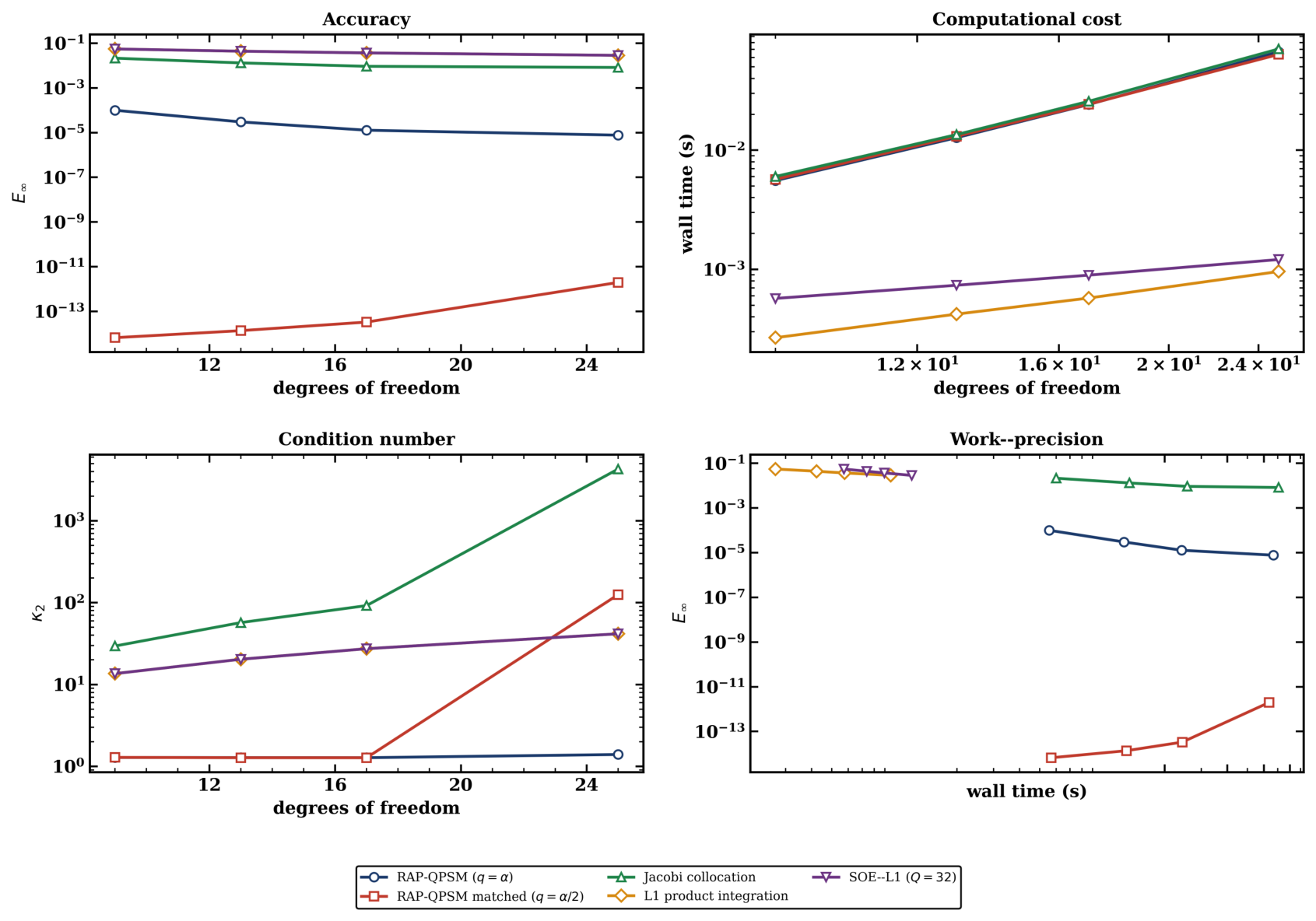
The representative accuracy, timing, and conditioning values at 17 degrees of freedom are summarised in

Table 5. Representative comparison at 17 degrees of freedom. The matched $q=\alpha /2$ row is an exact-on-space diagnostic and is not used for the generic cross-method accuracy claim.

Method	d.o.f.	${\mathit{E}}_{\mathit{\infty }}$	Time (ms)	${\mathit{\kappa }}_2$	${\mathit{\kappa }}_2\left({\mathcal{P}}^{-1}\mathcal{L}\right)$
RAP-QPSM ($q=\alpha$)	17	$1.283\times {10}^{-5}$	24.145	$2.571\times {10}^2$	$1.275$
RAP-QPSM, matched ($q=\alpha /2$)	17	$3.331\times {10}^{-14}$	24.279	$2.420\times {10}^4$	$1.272$
Jacobi collocation	17	$9.279\times {10}^{-3}$	25.693	$9.216\times {10}^1$	–
L1 product integration	17	$3.690\times {10}^{-2}$	0.575	$2.738\times {10}^1$	–
SOE–L1 ($Q=32$)	17	$3.690\times {10}^{-2}$	0.895	$2.738\times {10}^1$	–

.

At this resolution, the non-exact RAP-QPSM choice $q=\alpha$ is approximately three orders of magnitude more accurate than Jacobi collocation and more than three orders more accurate than the two low-order time-stepping variants. Its bare condition number is $2.571\times {10}^2$, while the proposed preconditioner reduces it to $1.275$. The matched $q=\alpha /2$ row reaches $3.331\times {10}^{-14}$, as predicted by exact-on-space representation, but also has a much larger bare condition number; preconditioning again reduces the latter to $1.272$. Low-order L1 is cheaper for this very small system, so accuracy versus wall time, rather than equal degrees of freedom alone, is the appropriate practical comparison.

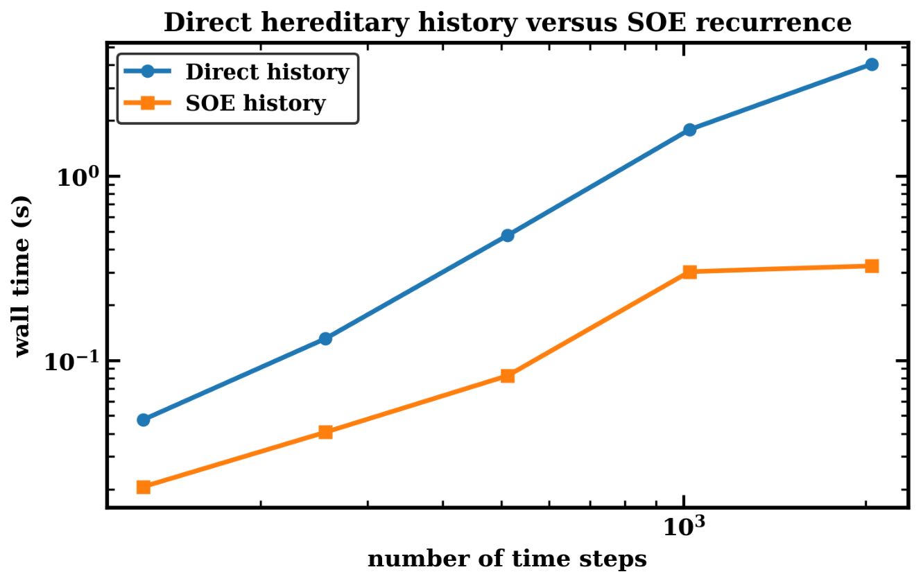
Figure 3 therefore reports not only accuracy, measured wall time, and conditioning versus degrees of freedom, but also a work–precision panel plotting $E_{\infty }$ directly against wall time and Figure 4 compares direct hereditary-history accumulation with the fixed-Q SOE recurrence, showing quadratic growth for the direct implementation and approximately linear growth for the fixed-mode recurrence.

A separate history-scaling experiment isolates the purpose of the SOE augmentation. At 2048 time steps, direct history accumulation requires $1.7637$ seconds, whereas the fixed-mode SOE recurrence requires $0.0865$ seconds, a factor of about $20.4$. Both retain the same underlying L1 discretisation error; the measured SOE kernel contribution is $1.06\times {10}^{-4}$. The corresponding measured values are reported in

Table 6. Direct and SOE hereditary-history implementations at 2048 steps.

Method	Steps	Time (s)	Error	Kernel Error
Direct history	2048	1.763681	0.001662	0
SOE history	2048	0.086535	0.001662	0.000106

.

Example 1 (Linear $\psi$-Caputo delay benchmark).

On $[0,4]$ with the identity clock $\psi \left(\xi \right)=\xi$ consider

$${{}^{\mathcal{C}}\mathfrak{D}}^{\alpha ;\psi }u\left(\xi \right)+u\left(\xi \right)+b_{0}u(\xi -\tau )=g\left(\xi \right),\alpha =0.6,\tau =0.3,b_0=0.35,$$

with the manufactured solution $u\left(\xi \right)=e^{-0.4\xi }cos\left(1.3\xi \right)$, history $\phi \left(\xi \right)=u\left(\xi \right)$ on $[-0.3,0]$, and forcing g obtained by inserting u into the left-hand side, the ψ-Caputo term being evaluated from a high-accuracy reference quadrature.

This is the cleanest test of the delay machinery. The numerical solution is obtained purely by assembling and inverting the operator $\mathcal{L}={\mathbb{D}}^{\left(\alpha \right)}+I+b_0{\mathbb{H}}_{\tau }$ with the initial-condition row, never by interpolating the known u.

Table 7. Example 1: Spectral convergence and conditioning.

N	${\mathit{E}}_{\mathit{\infty }}$	${\mathcal{R}}_{\mathit{\infty }}$	${\mathit{\kappa }}_{\mathit{L}}$	${\mathit{\kappa }}_{\mathit{P}}$
4	4.54 × ${10}^{-2}$	1.07 × ${10}^{-1}$	$4.2$	$1.26$
6	2.80 × ${10}^{-3}$	8.13 × ${10}^{-3}$	$6.7$	$1.31$
8	6.49 × ${10}^{-5}$	2.70 × ${10}^{-4}$	$9.8$	$1.33$
10	6.35 × ${10}^{-7}$	3.44 × ${10}^{-6}$	$13.5$	$1.37$
12	3.33 × ${10}^{-9}$	1.13 × ${10}^{-8}$	$18.2$	$1.37$
14	9.49e × ${10}^{-11}$	5.06 × ${10}^{-10}$	$22.7$	$1.38$
16	1.43e × ${10}^{-12}$	8.02 × ${10}^{-12}$	$27.5$	$1.37$
20	4.69 × ${10}^{-13}$	6.94 × ${10}^{-12}$	$38.9$	$1.37$
24	6.64 × ${10}^{-13}$	8.02 × ${10}^{-12}$	$1770.3$	$8.27$

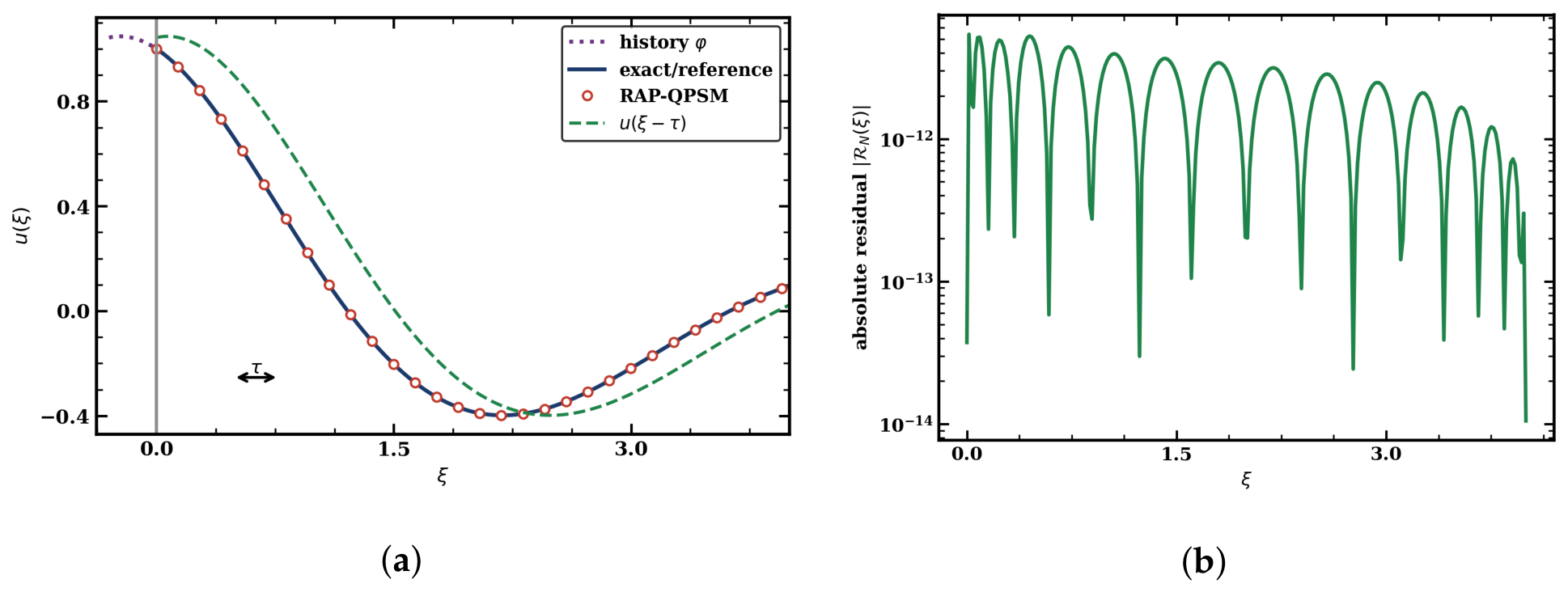
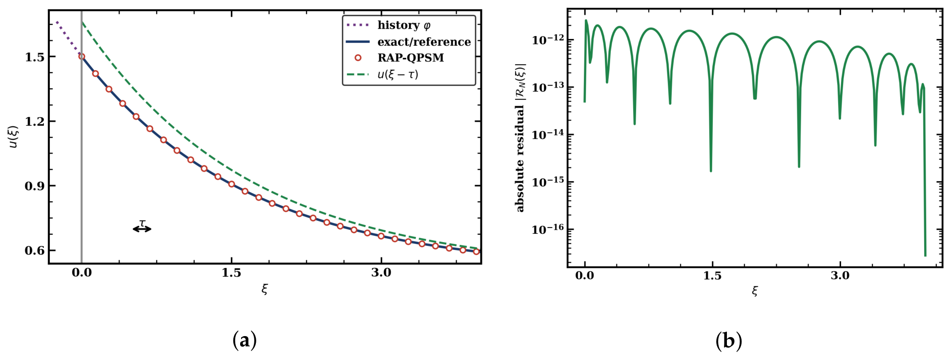
shows spectral convergence from $4.5\times {10}^{-2}$ at $N=4$ to $1.4\times {10}^{-12}$ at $N=16$, with the bare condition number growing slowly while the preconditioned condition number stays near $1.37$; the jump in ${\kappa }_L$ at $N=24$ is the onset of round-off saturation once the error has reached machine level. Figure 5 displays the solution together with the spectral approximation and the exact residual. 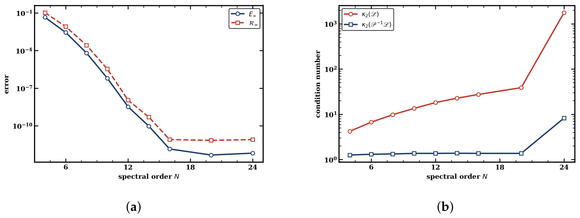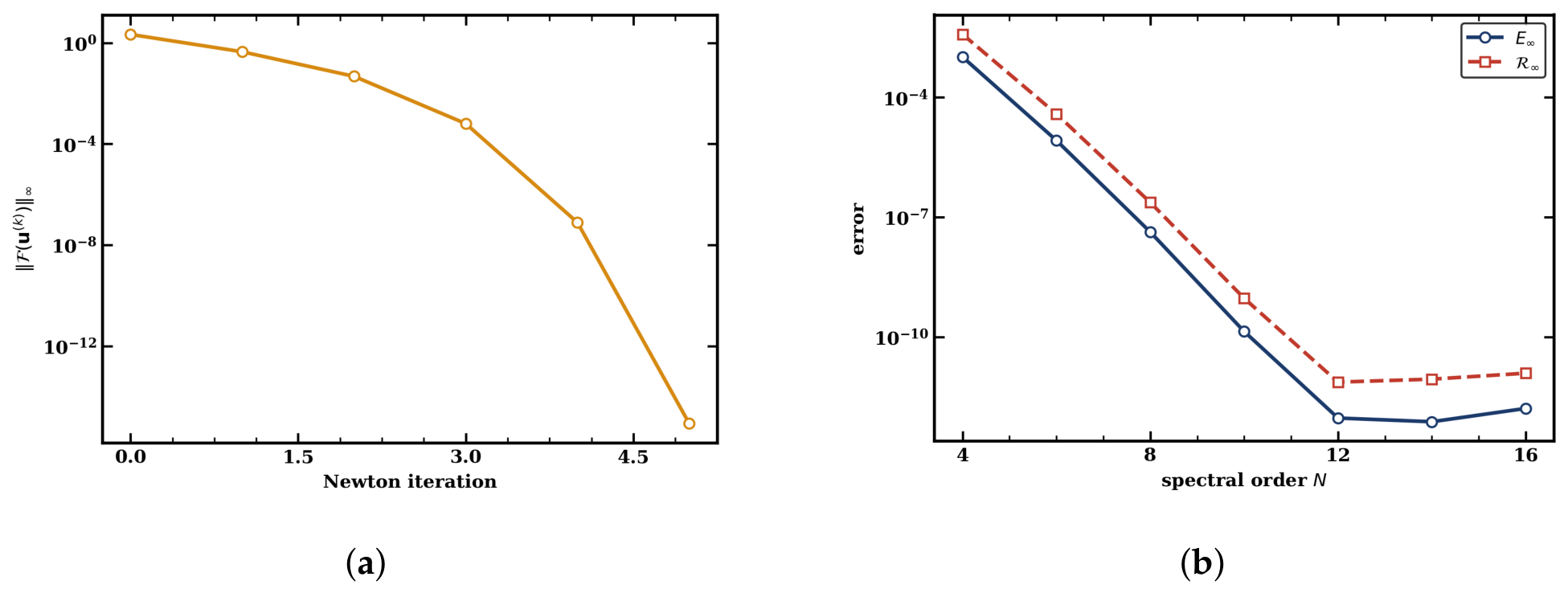To make the delay explicit, the solution panel also shows the history segment $\phi$ on $[a-\tau ,a]$, the $\tau$-shifted trace $u(\xi -\tau )$ that the delay term feeds back into the equation, and a labelled arrow of length $\tau$; the horizontal displacement between u and its shifted copy is the delay. The geometric error decay and the contrast between the bare and preconditioned condition numbers are shown in Figure 6.

Remark 10 (Reduction).

Setting $b_0=0$, $\lambda =0$ and $\psi \left(\xi \right)=\xi$ reduces (10) to the single-term Caputo equation solved by the quantum pseudo-spectral approach of [45]; the present scheme then reproduces that method, and the delay term is the genuine extension exercised here.

Example 2 (Multi-term two-order problem on a curved clock).

On $[0,3]$ with the curved clock $\psi \left(\xi \right)=\sqrt{1+\xi }$ consider the genuinely multi-term problem

$$\begin{array}{c}{{}^{\mathcal{C}}\mathfrak{D}}^{\alpha ;\psi }u+a_1{{}^{\mathcal{C}}\mathfrak{D}}^{\beta ;\psi }u+a_{0}u+b_{0}u(\xi -\tau )=g,\alpha =0.85,\beta =0.45,a_1=0.7,a_0=1,\\ b_0=0.25,\tau =0.4,\end{array}$$

with exact solution $u=cos(\pi \vartheta /2)+\frac{1}{2}\vartheta$ chosen smooth in the curved coordinate $\vartheta =(\psi \left(\xi \right)-\psi \left(0\right))/{\mathsf{\Psi }}_{♭}$.

This example exercises both the second fractional order $\beta$, for which Theorem 2 guarantees well-posedness, and a nontrivial memory clock.

Table 8. Example 2: Multi-term problem on the clock $\psi =\sqrt{1+\xi }$.

N	${\mathit{E}}_{\mathit{\infty }}$	${\mathcal{R}}_{\mathit{\infty }}$	${\mathit{\kappa }}_{\mathit{L}}$	${\mathit{\kappa }}_{\mathit{P}}$
4	4.10 × ${10}^{-4}$	5.10 × ${10}^{-3}$	$26.3$	$2.14$
6	1.50 × ${10}^{-6}$	3.36 × ${10}^{-5}$	$55.2$	$2.34$
8	3.15 × ${10}^{-9}$	1.10 × ${10}^{-7}$	$98.0$	$2.55$
10	2.37 × ${10}^{-11}$	1.85 × ${10}^{-9}$	$153.1$	$2.75$
12	1.55 × ${10}^{-11}$	1.87 × ${10}^{-9}$	$223.5$	$2.95$
14	6.95 × ${10}^{-11}$	2.16 × ${10}^{-9}$	$305.7$	$3.11$
16	2.27 × ${10}^{-11}$	1.91 × ${10}^{-9}$	$405.0$	$3.33$
18	2.73 × ${10}^{-11}$	1.84 × ${10}^{-9}$	$520.2$	$3.53$

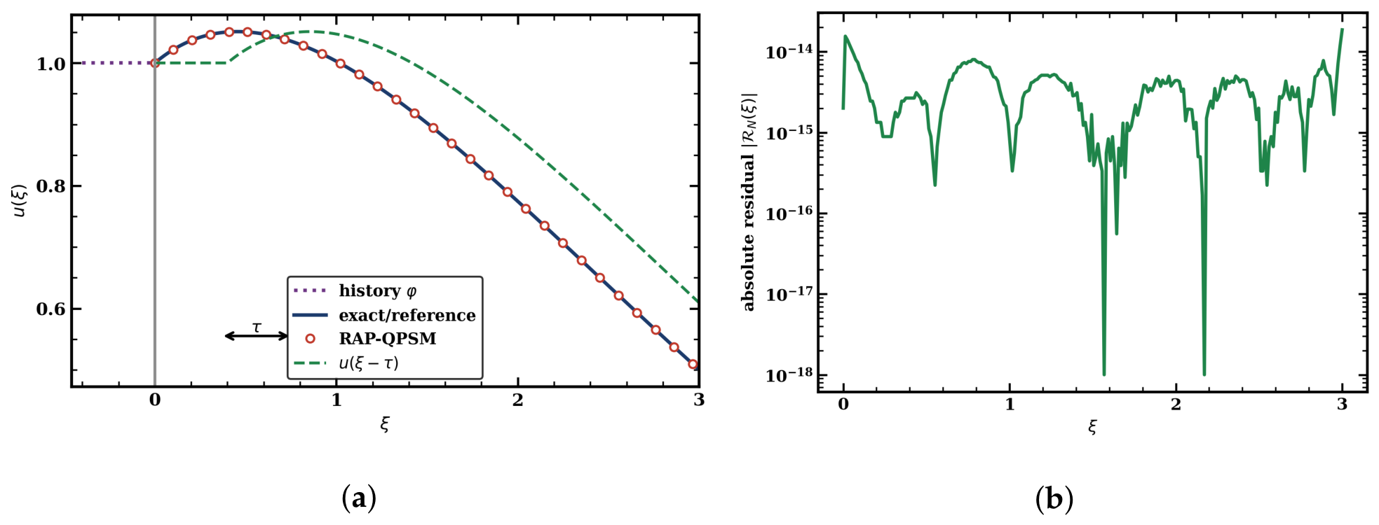
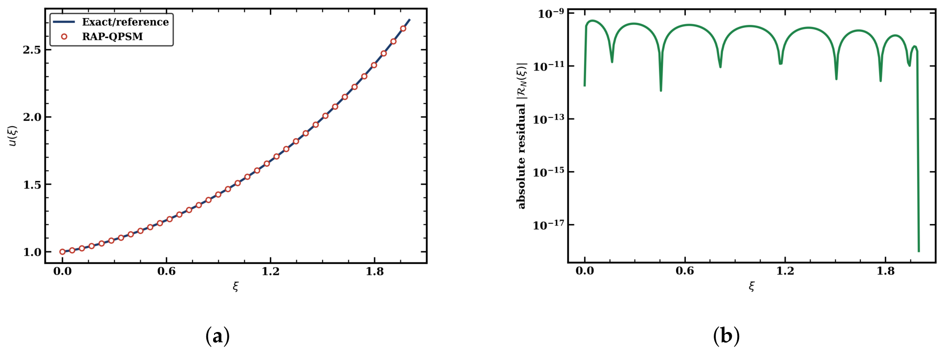
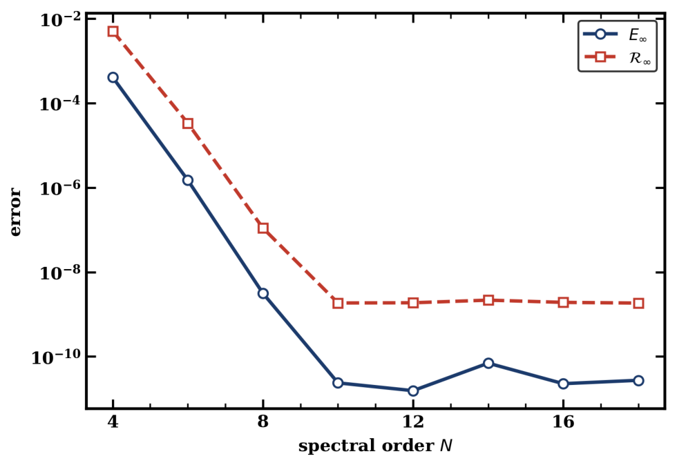
confirms spectral decay to about $2\times {10}^{-11}$ and a preconditioned condition number that remains below four while the bare one passes five hundred; Figure 7 shows the solution with its history and $\tau$-shifted trace alongside the exact residual, and Figure 8 the convergence history.

Remark 11 (Reduction).

With $a_1=0$, $b_0=0$ and $\psi \left(\xi \right)=\xi$, the problem collapses to the single-term Caputo benchmark of [45]; the second fractional order β and the curved clock ψ are the new ingredients.

Example 3 (Nonlinear Riccati-type delay equation).

On $[0,4]$ with $\psi \left(\xi \right)=\xi$ consider the nonlinear delay equation

$${{}^{\mathcal{C}}\mathfrak{D}}^{\alpha ;\psi }u\left(\xi \right)+u{\left(\xi \right)}^2+b_{0}u(\xi -\tau )=g\left(\xi \right),\alpha =0.7,\tau =0.25,b_0=0.05,$$

with exact solution $u\left(\xi \right)=0.5+e^{-0.6\xi }$ and history $\phi =u$ on $[-0.25,0]$. The quadratic term $F(\xi ,u)=u^2$ is treated at the nodes without a fractional chain rule.

The discrete system is solved by the damped Newton iteration of Algorithm 2, with the Jacobian carrying the exact diagonal ${\partial }_{u}F=2u$. The iteration converges quadratically, the residual passing through $1.17$, $2.20\times {10}^{-2}$, $2.58\times {10}^{-5}$, $8.69\times {10}^{-11}$, and $1.61\times {10}^{-15}$ in four steps independently of N (

Table 9. Example 3: Nonlinear delay problem, damped Newton.

N	${\mathit{E}}_{\mathit{\infty }}$	${\mathcal{R}}_{\mathit{\infty }}$	Newton Steps
4	1.03 × ${10}^{-3}$	3.81 × ${10}^{-3}$	4
6	8.36 × ${10}^{-6}$	3.86 × ${10}^{-5}$	4
8	4.24 × ${10}^{-8}$	2.34 × ${10}^{-7}$	4
10	1.37 × ${10}^{-10}$	9.27 × ${10}^{-10}$	4
12	9.25 × ${10}^{-13}$	7.36 × ${10}^{-12}$	4
14	7.47 × ${10}^{-13}$	8.72 × ${10}^{-12}$	4
16	1.61 × ${10}^{-12}$	1.23 × ${10}^{-11}$	4

). Figure 9 leads with the solution against the spectral approximation, with the history segment and the dashed $\tau$-shifted trace $u(\xi -\tau )$ making the delayed feedback visible, followed by the exact residual; the quadratic Newton history is shown separately in Figure 10.

Algorithm 2 Damped Newton Iteration for the Nonlinear Collocation System

1: Initialise ${\mathit{u}}^{\left(0\right)}$ satisfying the initial condition.   2: for  $k=0,1,2,\dots$ do   3:     form the residual $\mathit{R}\left({\mathit{u}}^{\left(k\right)}\right)$ from (10) using the exact matrices ${\mathbb{D}}^{\left(\alpha \right)},{\mathbb{D}}^{\left(\beta \right)},{\mathbb{H}}_{\tau },\mathbb{M}$;   4:     if ${∥\mathit{R}\left({\mathit{u}}^{\left(k\right)}\right)∥}_{\infty }<\mathrm{tol}$ then   5:         stop   6:     end if   7:     form the Jacobian $\mathit{J}\left({\mathit{u}}^{\left(k\right)}\right)=\mathcal{L}+diag\left({\partial }_{u}F\right)$ with the unit initial-condition row;   8:     solve $\mathit{J}\Delta \mathit{u}=-\mathit{R}$ (preconditioned by $\mathcal{P}$);   9:     backtrack $\theta \in (0,1]$ until the residual merit decreases and set ${\mathit{u}}^{(k+1)}={\mathit{u}}^{\left(k\right)}+\theta \Delta \mathit{u}$. 10: end for

Remark 12 (Reduction).

Removing the delay ($b_0=0$) leaves a nonlinear single-term Caputo equation handled at nodes without a fractional chain rule, exactly as in [45]; the delayed feedback is the extension.

Example 4 (Weakly singular $\psi$-memory and kernel compression).

On $[0,2]$, with the power clock $\psi \left(\xi \right)={\xi }^{1.3}$, consider the memory equation

$${{}^{\mathcal{C}}\mathfrak{D}}^{\alpha ;\psi }u\left(\xi \right)+u\left(\xi \right)+\lambda {\mathcal{M}}_{\psi ,\nu }u\left(\xi \right)=g\left(\xi \right),\alpha =0.65,\nu =0.3,\lambda =0.8,$$

with weakly singular kernel ${(\psi \left(\xi \right)-\psi \left(s\right))}^{-\nu }$ and exact solution $u=e^{\vartheta }$ smooth in the coordinate $\vartheta =\psi \left(\xi \right)/\psi \left(2\right)$.

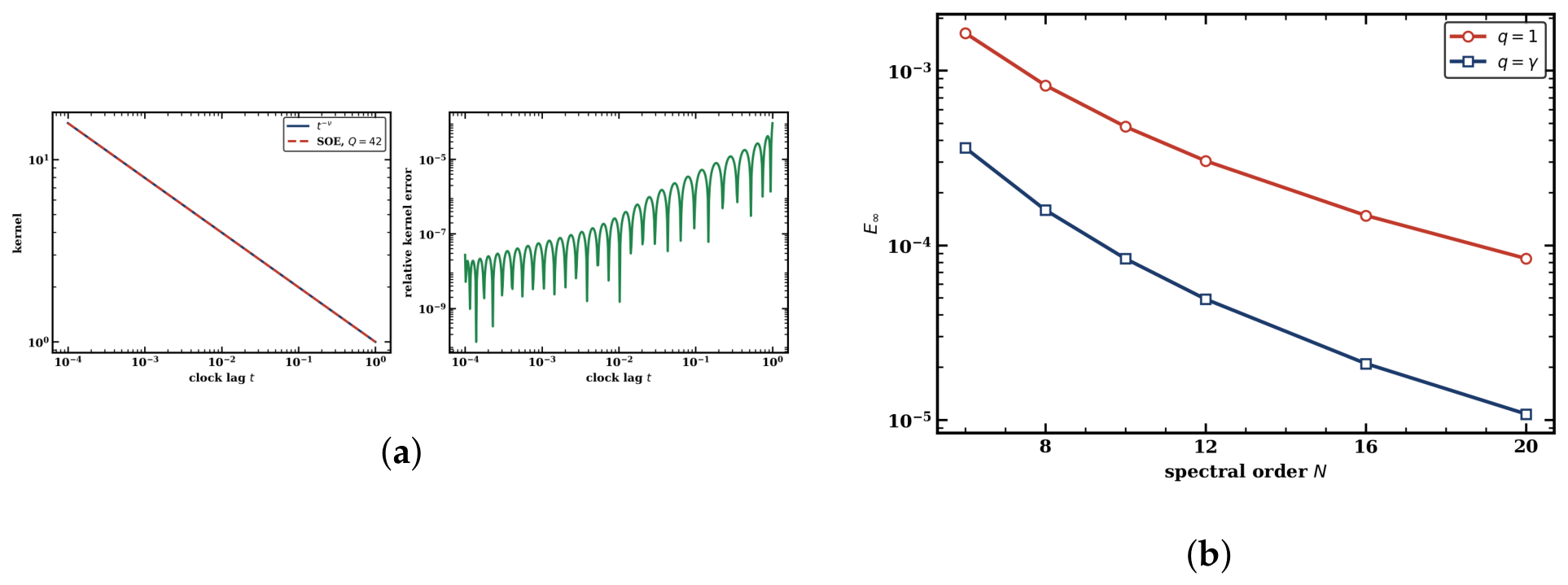
This example isolates the hereditary memory and its compression. The exact memory matrix of Lemma 6 delivers spectral accuracy (Table 10), shown together with the solution and the exact residual in Figure 11. The sum-of-exponentials compression of Lemma 7 is reported in Table 11: the kernel error falls from $3.0\times {10}^{-3}$ with $Q=18$ modes to $6.1\times {10}^{-14}$ with $Q=100$ modes, and the action of the compressed memory on the computed solution matches the exact memory to a relative $6.84\times {10}^{-4}$ at $Q=42$ over the tested values of N. This is the fixed-accuracy regime of Proposition 3: once the target kernel tolerance is prescribed, the same local mode set can be reused as N varies. It is not a claim that Q remains constant when the kernel tolerance is itself tightened spectrally with N; see Remark 4. Table 12 examines the basis exponent of Remark 2 on the genuinely singular profile ${\vartheta }^{1.3}+0.4{\vartheta }^2$, showing that matching q to the leading fractional exponent improves the accuracy by a factor between three and eight; it does not by itself restore full spectral decay, because the second term of the profile is not simultaneously a polynomial in ${\vartheta }^q$, which is the regime that motivates the multidomain treatment of Example 5. The SOE kernel fit and the basis-exponent comparison are displayed in Figure 12.

Table 10. Example 4: Convergence.

N	${\mathit{E}}_{\mathit{\infty }}$	${\mathcal{R}}_{\mathit{\infty }}$
4	6.39 × ${10}^{-5}$	2.08 × ${10}^{-4}$
6	9.44 × ${10}^{-8}$	4.48 × ${10}^{-7}$
8	8.23 × ${10}^{-11}$	5.16 × ${10}^{-10}$
10	6.56 × ${10}^{-12}$	1.47 × ${10}^{-10}$
12	3.54 × ${10}^{-11}$	1.40 × ${10}^{-10}$
14	9.36 × ${10}^{-12}$	1.43 × ${10}^{-10}$

Table 10. Example 4: Convergence.

N	${\mathit{E}}_{\mathit{\infty }}$	${\mathcal{R}}_{\mathit{\infty }}$
4	6.39 × ${10}^{-5}$	2.08 × ${10}^{-4}$
6	9.44 × ${10}^{-8}$	4.48 × ${10}^{-7}$
8	8.23 × ${10}^{-11}$	5.16 × ${10}^{-10}$
10	6.56 × ${10}^{-12}$	1.47 × ${10}^{-10}$
12	3.54 × ${10}^{-11}$	1.40 × ${10}^{-10}$
14	9.36 × ${10}^{-12}$	1.43 × ${10}^{-10}$

Table 11. Example 4: SOE.

Q	Kernel Error
18	3.01 × ${10}^{-3}$
32	2.08 × ${10}^{-4}$
52	3.05 × ${10}^{-6}$
74	3.49 × ${10}^{-9}$
100	6.06 × ${10}^{-14}$

Table 11. Example 4: SOE.

Q	Kernel Error
18	3.01 × ${10}^{-3}$
32	2.08 × ${10}^{-4}$
52	3.05 × ${10}^{-6}$
74	3.49 × ${10}^{-9}$
100	6.06 × ${10}^{-14}$

Table 12. Example 4: q-match.

N	q = 1	q = $\mathit{\gamma }$
6	1.64 × ${10}^{-3}$	3.61 × ${10}^{-4}$
8	8.23 × ${10}^{-4}$	1.59 × ${10}^{-4}$
10	4.77 × ${10}^{-4}$	8.37 × ${10}^{-5}$
12	3.04 × ${10}^{-4}$	4.91 × ${10}^{-5}$
16	1.48 × ${10}^{-4}$	2.10 × ${10}^{-5}$
20	8.39 × ${10}^{-5}$	1.08 × ${10}^{-5}$

Table 12. Example 4: q-match.

N	q = 1	q = $\mathit{\gamma }$
6	1.64 × ${10}^{-3}$	3.61 × ${10}^{-4}$
8	8.23 × ${10}^{-4}$	1.59 × ${10}^{-4}$
10	4.77 × ${10}^{-4}$	8.37 × ${10}^{-5}$
12	3.04 × ${10}^{-4}$	4.91 × ${10}^{-5}$
16	1.48 × ${10}^{-4}$	2.10 × ${10}^{-5}$
20	8.39 × ${10}^{-5}$	1.08 × ${10}^{-5}$

Remark 13 (Reduction).

For $\lambda =0$, $\psi \left(\xi \right)=\xi$ and integer $q=1$, the problem is the polynomial Caputo benchmark of [45]; the weakly singular memory and its compression are the new structure, and the q-matching clarifies when the polynomial basis is and is not adequate.

Example 5 (Singularly perturbed delay problem).

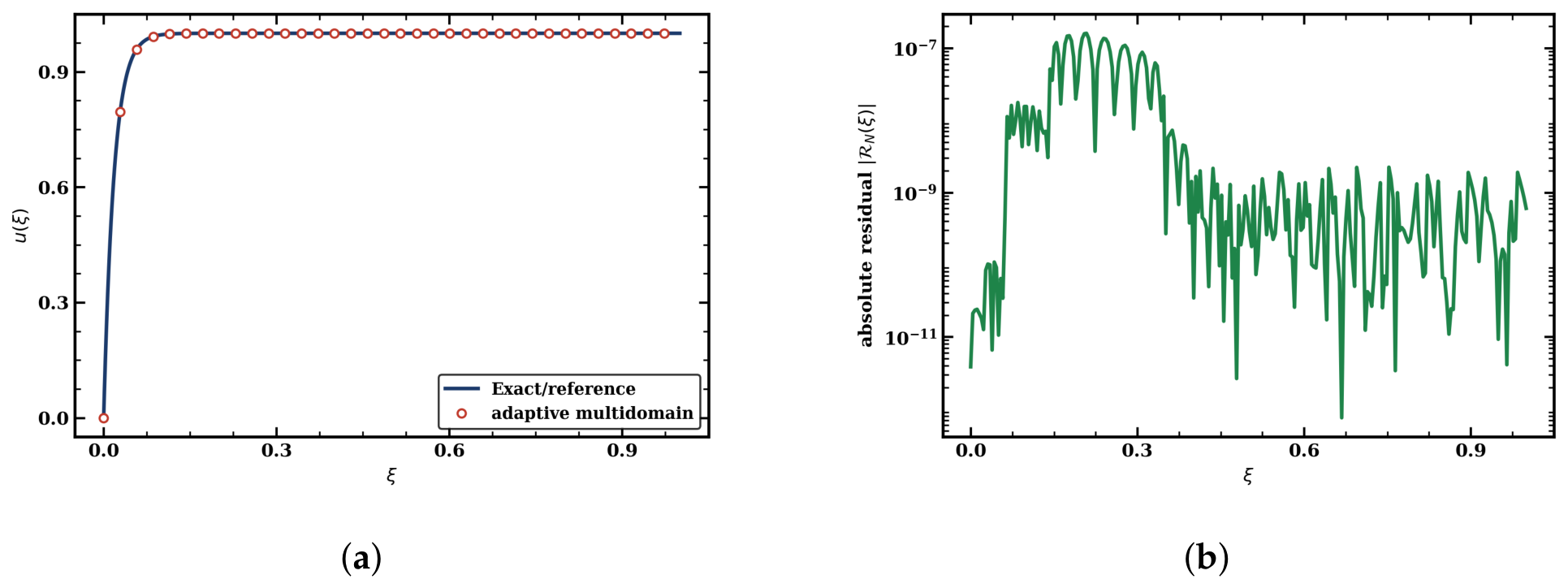
On $[0,1]$, with $\psi \left(\xi \right)=\xi$, consider the singularly perturbed delay problem

$$\epsilon {{}^{\mathcal{C}}\mathfrak{D}}^{\alpha ;\psi }u\left(\xi \right)+u\left(\xi \right)+b_{0}u(\xi -\tau )=g\left(\xi \right),\alpha =0.7,\tau =0.05,b_0=0.1,$$

with a small parameter ε multiplying the principal derivative and a forcing producing a steep boundary layer near $\xi =0$. The delay $\tau =0.05$ is short relative to the domain, so the layer rather than the delay dominates the figures.

This is the showcase for the preconditioner and the adaptive solver. Figure 13 shows the layer-resolving solution against the reference and the exact residual. Table 13 reports the conditioning at $N=28$ as $\epsilon$ varies: at $\epsilon =1$, the bare condition number is $1.68\times {10}^7$ and the preconditioner brings it to $1.49\times {10}^2$, about five orders of magnitude, and the benefit is largest in the derivative-dominated regime exactly as Remark 8 predicts. Table 14 shows the same effect as the order grows at fixed $\epsilon ={10}^{-3}$. 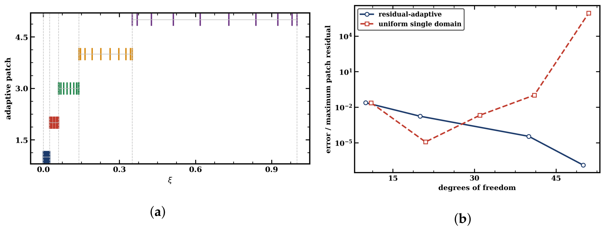Table 15 documents the residual-adaptive multidomain solver driving the residual from $2.4\times {10}^{-2}$ on one patch to $1.3\times {10}^{-7}$ on five patches and fifty degrees of freedom, while Table 16 shows that uniform single-domain refinement is erratic and ultimately diverges through round-off; Figure 14 shows the layer-resolving node distribution and the efficiency comparison.

Table 13. Example 5: Conditioning versus $\epsilon$ at $N=28$.

$\mathit{\epsilon }$	${\mathit{\kappa }}_{\mathit{L}}$	${\mathit{\kappa }}_{\mathit{P}}$
1	1.68 × ${10}^7$	1.49 × ${10}^2$
$0.1$	7.11 × ${10}^6$	2.66 × ${10}^3$
$0.01$	1.07 × ${10}^6$	4.97 × ${10}^3$
$0.001$	2.79 × ${10}^4$	2.78 × ${10}^2$
$0.0001$	2.28 × ${10}^2$	3.51 × ${10}^9$

Table 13. Example 5: Conditioning versus $\epsilon$ at $N=28$.

$\mathit{\epsilon }$	${\mathit{\kappa }}_{\mathit{L}}$	${\mathit{\kappa }}_{\mathit{P}}$
1	1.68 × ${10}^7$	1.49 × ${10}^2$
$0.1$	7.11 × ${10}^6$	2.66 × ${10}^3$
$0.01$	1.07 × ${10}^6$	4.97 × ${10}^3$
$0.001$	2.79 × ${10}^4$	2.78 × ${10}^2$
$0.0001$	2.28 × ${10}^2$	3.51 × ${10}^9$

Table 14. Example 5: Conditioning versus N at $\epsilon ={10}^{-3}$.

N	${\mathit{\kappa }}_{\mathit{L}}$	${\mathit{\kappa }}_{\mathit{P}}$
8	1.12 × ${10}^0$	1.14 × ${10}^0$
16	1.21 × ${10}^0$	1.21 × ${10}^0$
24	1.26 × ${10}^0$	1.25 × ${10}^0$
28	2.79 × ${10}^4$	2.78 × ${10}^2$
32	9.34 × ${10}^9$	7.98 × ${10}^6$

Table 14. Example 5: Conditioning versus N at $\epsilon ={10}^{-3}$.

N	${\mathit{\kappa }}_{\mathit{L}}$	${\mathit{\kappa }}_{\mathit{P}}$
8	1.12 × ${10}^0$	1.14 × ${10}^0$
16	1.21 × ${10}^0$	1.21 × ${10}^0$
24	1.26 × ${10}^0$	1.25 × ${10}^0$
28	2.79 × ${10}^4$	2.78 × ${10}^2$
32	9.34 × ${10}^9$	7.98 × ${10}^6$

Table 15. Example 5: Residual-adaptive multidomain ($\epsilon ={10}^{-2}$).

Level	Patches	D.O.F.	${max}_{\mathit{m}}{\mathit{r}}_{\mathit{m}}$
0	1	10	2.39 × ${10}^{-2}$
1	2	20	1.73 × ${10}^{-3}$
2	4	40	3.47 × ${10}^{-5}$
3	5	50	1.30 × ${10}^{-7}$

Table 15. Example 5: Residual-adaptive multidomain ($\epsilon ={10}^{-2}$).

Level	Patches	D.O.F.	${max}_{\mathit{m}}{\mathit{r}}_{\mathit{m}}$
0	1	10	2.39 × ${10}^{-2}$
1	2	20	1.73 × ${10}^{-3}$
2	4	40	3.47 × ${10}^{-5}$
3	5	50	1.30 × ${10}^{-7}$

Table 16. Example 5: Uniform single domain.

D.O.F.	${\mathit{E}}_{\mathit{\infty }}$
11	2.34 × ${10}^{-2}$
21	1.17 × ${10}^{-5}$
31	2.10 × ${10}^{-3}$
41	1.04 × ${10}^{-1}$
51	8.71 × ${10}^5$

Table 16. Example 5: Uniform single domain.

D.O.F.	${\mathit{E}}_{\mathit{\infty }}$
11	2.34 × ${10}^{-2}$
21	1.17 × ${10}^{-5}$
31	2.10 × ${10}^{-3}$
41	1.04 × ${10}^{-1}$
51	8.71 × ${10}^5$

Remark 14 (Reduction).

At $\epsilon =1$, $b_0=0$ on a single domain, the problem is a standard single-term Caputo equation; the singular perturbation, the delay, and the multidomain adaptivity are the features that the bare quantum pseudo-spectral method of [45] does not address.

Example 6 (Nonlinear fractional population model with memory clocks).

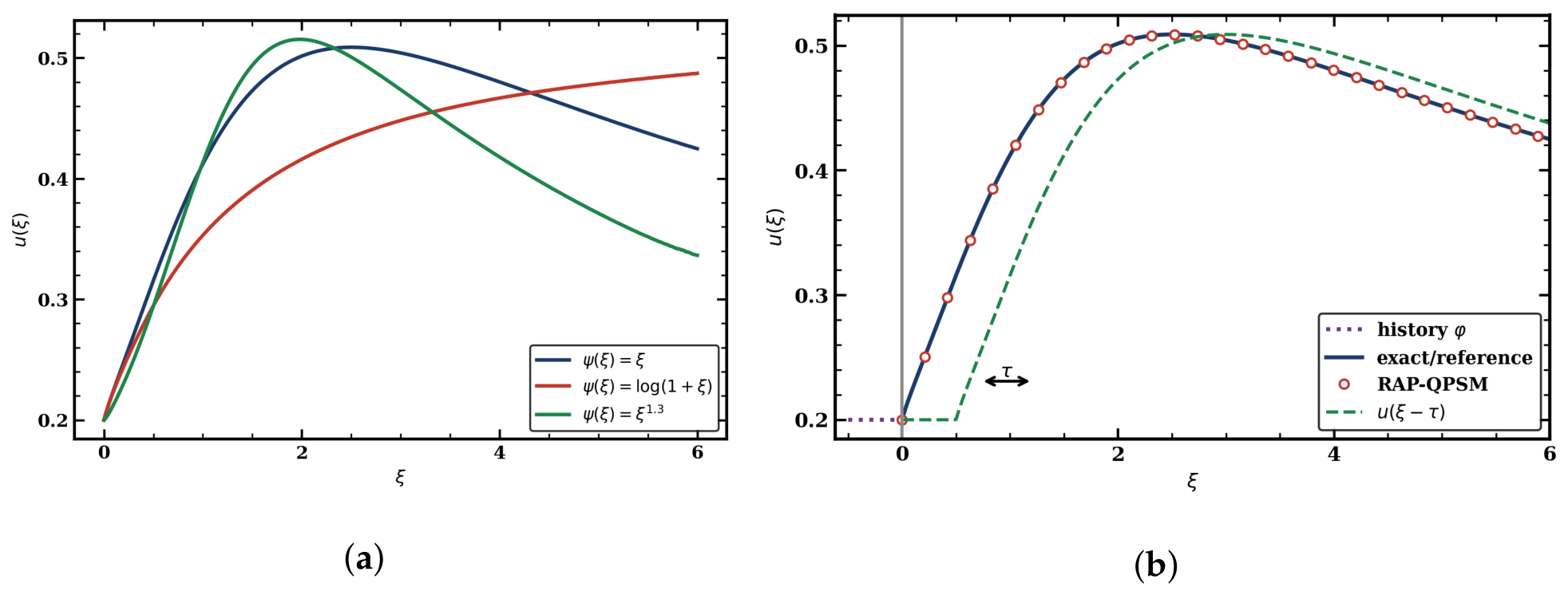
On $[0,6]$, solve the nonlinear hereditary population model

$${{}^{\mathcal{C}}\mathfrak{D}}^{\alpha ;\psi }u\left(\xi \right)=ru\left(1-{\displaystyle \frac{u}{\mathcal{K}}}\right)-\chi u\left(\xi \right){\mathcal{M}}_{\psi ,\nu }u\left(\xi \right)-hu(\xi -\tau ),$$

(27)

with $\alpha =0.85$, $\nu =0.4$, $r=1.4$, $\mathcal{K}=1$, $\chi =0.25$, $h=0.3$, $\tau =0.5$ and constant history $u\equiv 0.2$, where the memory term models a hereditary crowding pressure and the delayed term a maturation loss.

The parameter choices are nondimensional scale choices intended to isolate the three memory clocks. The carrying capacity $\mathcal{K}=1$ normalises population density, so the history level $u_0=0.2$ represents $20\%$ of carrying capacity. The intrinsic rate $r=1.4$ gives visible logistic recovery on the observation interval. The coefficient $\chi =0.25$ represents moderate hereditary crowding: accumulated past population reduces current growth without dominating the instantaneous logistic term. The delayed-loss coefficient $h=0.3$ and lag $\tau =0.5$ model a moderate maturation, harvesting, or feedback delay. These values are illustrative and are held fixed so that changes among the identity, logarithmic, and power clocks can be attributed to the memory clock rather than parameter recalibration. A biological application would require fitting $r,\chi ,h$, and $\tau$ to data and reporting parameter uncertainty.

There is no closed-form solution, so the bespoke Newton iteration, whose Jacobian carries the memory-product term $\chi [diag(\mathbb{M}\mathit{u})+diag(\mathit{u}\left)\mathbb{M}\right]$, certifies the result by its residual, and accuracy is assessed by self-convergence under three different memory clocks in Table 17. The clock changes the dynamics measurably, and the iteration converges in five to seven steps in every case. 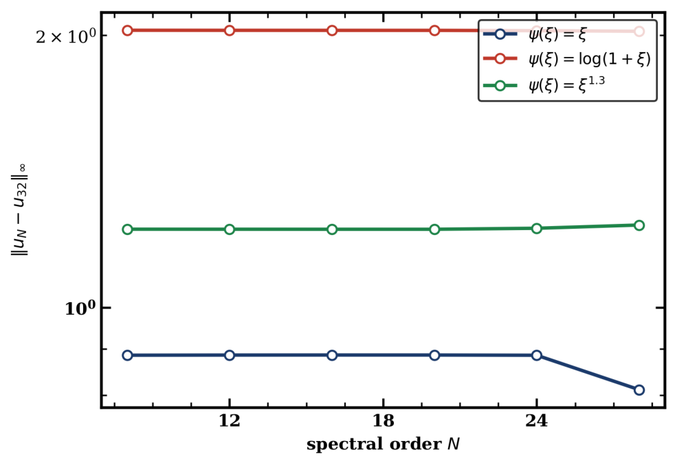Figure 15 shows the trajectories under the three clocks together with the delayed trace $u(\xi -\tau )$ for the identity clock, which makes the maturation delay explicit, and Figure 16 shows the self-convergence.

It is worth distinguishing the two accuracy measures, which quantify different things. Table 17 reports the fixed-step self-convergence ${\left|\right|u_{18}-u_{24}\left|\right|}_{\infty }$, the change in the computed trajectory between two specific resolutions $N=18$ and $N=24$, which is around ${10}^{-3}$. Figure 16 instead plots the running self-convergence ${\left|\right|u_N-u_{32}\left|\right|}_{\infty }$ against a finer reference $N=32$ as N increases, so its vertical scale spans the whole decay from coarse to fine and is naturally larger at small N; the two are therefore consistent rather than contradictory, the table being one slice of the curve.

Table 17. Example 6: Fixed-step self-convergence ${∥u_{18}-u_{24}∥}_{\infty }$ and Newton steps for three memory clocks.

Memory Clock $\mathit{\psi }$	${∥{\mathit{u}}_{18}-{\mathit{u}}_{24}∥}_{\mathit{\infty }}$	Newton Steps
$\psi =\xi$	8.37 × ${10}^{-4}$	6
$\psi =log(1+\xi )$	2.39 × ${10}^{-3}$	5
$\psi ={\xi }^{1.3}$	5.00 × ${10}^{-3}$	7

Table 17. Example 6: Fixed-step self-convergence ${∥u_{18}-u_{24}∥}_{\infty }$ and Newton steps for three memory clocks.

Memory Clock $\mathit{\psi }$	${∥{\mathit{u}}_{18}-{\mathit{u}}_{24}∥}_{\mathit{\infty }}$	Newton Steps
$\psi =\xi$	8.37 × ${10}^{-4}$	6
$\psi =log(1+\xi )$	2.39 × ${10}^{-3}$	5
$\psi ={\xi }^{1.3}$	5.00 × ${10}^{-3}$	7

Remark 15 (Reduction).

Setting $\chi =0$ and $h=0$ with $\psi \left(\xi \right)=\xi$ reduces (27) to a nonlinear logistic Caputo equation of the type treated at nodes in [45]; the hereditary crowding, the delayed loss, and the tunable memory clock are the extensions.

10. Results and Discussion

The numerical section contains six model studies and a separate four-method benchmark. The model studies connect the analytical claims to smooth, singular, layered, delayed, hereditary, and nonlinear examples, whereas the benchmark isolates accuracy, measured cost, conditioning, and history scaling relative to Jacobi collocation and L1-type schemes.

The convergence claim of Remark 2 is borne out in two complementary ways. When the solution is smooth in the coordinate $\vartheta$, as in Examples 1, 2, 3, and 4, the error and the residual fall geometrically until they saturate at machine precision, reaching $1.4\times {10}^{-12}$ at $N=16$ in the linear benchmark and $8\times {10}^{-11}$ at $N=8$ in the weakly singular problem; this is the exact-on-space property of the operational matrices in action: for the represented spectral approximation, the interior nodal $\psi$-Caputo derivative is evaluated exactly, and the unit-kernel memory operator is evaluated exactly on the same finite basis. When instead, the solution carries a genuine fractional power, the q-matching study of Table 12 shows that aligning the basis exponent with the leading singularity reduces the error by a factor between three and eight across the whole range of N. The improvement is real but does not by itself restore full spectral decay, because the secondary term of the test profile is not simultaneously a polynomial in ${\vartheta }^q$; the honest reading is that the basis exponent should be matched to the dominant singular exponent, and that several incommensurate exponents call for the multidomain treatment instead. This is precisely the regime in which Example 5 operates.

The structured locality of Proposition 3 and the local-plus-history estimate of Theorem 3 explain the kernel-compression results. At a prescribed kernel tolerance, the SOE surrogate reproduces the far-history kernel with a mode count that can be reused across spectral orders, while the polynomial correction controls the singular interval that cannot be covered uniformly by an SOE fit as $\nu \to 1^{-}$. Remark 4 separates this fixed-accuracy statement from the asymptotic regime in which the kernel tolerance is tightened with N and Q must grow. Corollary 1 closes the theoretical loop by adding the SOE, near-field, and quadrature contributions to the exact residual. The sequential scaling test in Figure 4 confirms the corresponding computational transition: direct history grows quadratically, whereas fixed-mode SOE history is approximately linear.

The quantum statement must be read together with Figure 2, Table 4, and Section 6.2. Theorem 4 concerns preparation of an amplitude-encoded solution state under explicit block-encoding and right-hand-side assumptions. It does not include QRAM construction, fault-tolerant synthesis, or full classical readout. The adaptive partition is chosen classically; a quantum solve is performed only after the patch boundaries and oracle data are fixed. At fixed kernel accuracy, the SOE augmentation removes the N-growing global-history coupling; when the kernel tolerance is tightened with N, the resulting growth of Q must also be included. The spectral differentiation normalisation and the end-to-end data interface remain important implementation costs.

The comparative benchmark gives a deliberately qualified practical assessment. At 17 degrees of freedom, the non-exact RAP-QPSM choice $q=\alpha$ attains $1.283\times {10}^{-5}$ error, compared with $9.279\times {10}^{-3}$ for Jacobi collocation and $3.690\times {10}^{-2}$ for L1 and SOE–L1. The matched diagnostic $q=\alpha /2$ attains $3.331\times {10}^{-14}$ because the manufactured solution then lies in the finite basis space; this row demonstrates exact-on-space q-matching and is not used to claim generic superiority. The low-order L1 solve is faster at this small dimension, and the work–precision panel of Figure 3 displays that tradeoff directly. The preconditioner lowers the $q=\alpha$ RAP-QPSM condition number from $2.571\times {10}^2$ to $1.275$ and the matched-row condition number from $2.420\times {10}^4$ to $1.272$. These results identify, rather than universalise, the regimes in which high-order approximation, basis matching, conditioning control, and long-history compression are advantageous.

The conditioning interpretation of Remark 8 is confirmed sharply by Example 5. Table 13 shows that the preconditioner is most effective exactly where it is most needed, namely, in the derivative-dominated regime: at $\epsilon =1$, it reduces the condition number from $1.68\times {10}^7$ to $1.49\times {10}^2$, five orders of magnitude, and even in the worst intermediate case, the preconditioned condition number stays below the bare one by two to three orders. Table 14 shows the same mechanism along the order axis: once the spectral differentiation of a steep layer makes the bare operator ill conditioned, the preconditioner recovers a moderate condition number. This is the perturbation bound of Theorem 5 made visible, with the preconditioner reproducing the part of the operator responsible for the growth. The companion adaptive results of Table 15 and Table 16 make the practical case for the multidomain strategy: the residual-adaptive solver of Algorithm 1 reaches a residual of $1.3\times {10}^{-7}$ with five patches and fifty degrees of freedom, while uniform single-domain refinement is non-monotone and eventually diverges through round-off, the error rising to $8.7\times {10}^5$ at fifty-one degrees of freedom. The a posteriori control of Theorem 6 is what makes the refinement reliable, since the patchwise residual indicator is a computable surrogate for the error.

The multi-term theorem is exercised by Example 2, where a variable-coefficient lower-order fractional term is treated without commuting that coefficient through a fractional integral. Examples 3 and 6 exercise the nonlinear Newton systems, while the latter also show how distinct memory clocks alter a nondimensional hereditary population trajectory. Together with the comparative and resource studies, the experiments support three specific conclusions: the basis is highly accurate when it matches the clock-coordinate regularity; SOE localisation and preconditioning control different computational bottlenecks; and the quantum result is meaningful only under the stated oracle, state preparation, and fixed-partition assumptions.

11. Conclusions

We introduced a $\psi$-Caputo pseudo-spectral framework for differential equations containing both discrete delay and weakly singular hereditary memory. The two structural steps that make the discretisation suitable for a quantum linear-system formulation are the SOE localisation of the history and the structure-preserving preconditioner. The operational matrices are exact on the represented finite spectral space, while the local-plus-history estimate quantifies the separate spectral, kernel-compression, near-field, quadrature, and residual contributions.

The experiments show that the q-adapted basis can deliver substantially higher accuracy per degree of freedom than integer-power Jacobi collocation and low-order L1 product integration. They also confirm that the preconditioner keeps ${\kappa }_2\left({\mathcal{P}}^{-1}\mathcal{L}\right)$ close to one in the comparative test and that for a prescribed kernel tolerance, fixed-mode SOE history reduces long-history cost without altering the underlying L1 discretisation error. When the kernel tolerance is required to decay spectrally with N, the mode count must grow according to Remark 4.

The quantum result is stated as a solution-state preparation complexity under explicit block-encoding, normalisation, and right-hand-side preparation assumptions, with the effective inverse parameter ${\kappa }_{\mathrm{eff}}={\alpha }_B{∥B^{-1}∥}_2$ kept distinct from the ordinary matrix condition number. The residual-adaptive partition is a classical outer loop; once its boundaries are fixed, the local patch operators, transferred memory modes, and sparse interface rows admit a patch-selected block encoding.

Future work will develop end-to-end fault-tolerant resource estimates, optimised near-field circuits, and calibrated delay–memory applications. These directions concern hardware realisation and model identification beyond the mathematical and numerical framework established here.