Path-Dependent Landslide Initiation Through Response-Generated Memory Under Mainshock–Aftershock Loading

Abstract

Earthquake sequences can affect slope stability before recovery from an earlier event is complete, yet reduced-order models commonly treat successive earthquakes as independent inputs or prescribe cumulative damage through event-based increments. We introduce a bounded, response-generated memory state into a delayed two-block landslide model. The state reduces incremental friction, evolves exclusively through computed dissipative response, and heals continuously between earthquakes. Its critical value is derived independently from the characteristic roots of the delayed mechanical subsystem. Paired aftershock-only and mainshock–aftershock experiments use corrected accelerograms from the 2011 Redcliffs sequence as recorded inputs rather than calibration data. Across 1255 admissible deterministic comparisons, a subcritical mainshock reduced the aftershock activation threshold in every parameter cell; 1235 threshold intervals were strictly separated, while 20 converged to the aftershock-only limit under strong healing. Threshold reduction was almost entirely determined by retained memory (Spearman rank coefficient ρS = 0.9997). Under stochastic forcing, all 33 primary parameter cells showed the same direction of reduction, and 32 paired 95% bootstrap confidence intervals excluded zero. Independent 4096-realisation ensembles yielded reductions of 18.0–26.2% under white-noise and Ornstein–Uhlenbeck forcing. Resetting memory reproduced the aftershock-only response exactly, whereas removing displacement delay eliminated delayed activation. These results identify a causal mechanism by which a non-activating earthquake can transiently lower the activation threshold of a subsequent event, while distinguishing dimensionless model activation from physical landslide failure.

1. Introduction

Earthquake-triggered landslides are commonly analysed as consequences of individual earthquakes, yet damaging seismic crises frequently occur as sequences rather than isolated events. In such sequences, a later earthquake may act on a slope whose mechanical state has not recovered from the preceding shock. Fracture networks, stress redistribution, pore-pressure conditions, and shear-zone properties may all remain transiently altered long after ground shaking has ceased. Regional inventories and remote-sensing studies increasingly document cumulative landslide activity, spatial preconditioning, and reactivation associated with successive earthquakes [1,2,3,4]. These observations suggest that treating successive earthquakes as mechanically independent is not always justified, particularly when the characteristic recovery time of the slope is comparable to the interval separating seismic events.

Several established modelling frameworks have addressed different aspects of the sequence problem. Newmark-type sliding-block methods remain the foundation for estimating coseismic displacement and regional landslide susceptibility [5,6,7]. More recent studies have investigated mainshock–aftershock sequences using recorded earthquake pairs, centrifuge experiments, continuum simulations, empirical displacement relationships, spatial random fields, and probability-density evolution [8,9,10,11,12]. A recent reliability framework further evaluates permanent displacement using collections of recorded mainshock–aftershock sequences [13]. Collectively, these studies demonstrate that earthquake sequences may produce substantially larger cumulative displacement or damage than individual events. However, increased response under a concatenated sequence does not by itself establish why the later earthquake becomes more effective. The additional response may simply reflect the additional seismic input rather than a persistent change in the mechanical state of the slope. Consequently, the central unresolved issue is not whether earthquake sequences produce larger responses, but whether the state inherited from a non-activating earthquake can itself be identified as the causal mechanism responsible for lowering the activation threshold of a subsequent event.

A variety of physical mechanisms capable of storing such inherited state have already been identified. Repeated dynamic loading progressively damages rock masses and slopes [14,15,16], while experimental and numerical studies of the Xinmo landslide, a well-documented 2017 case in China used to investigate progressive seismic damage, reveal multistage damage accumulation and progressive failure under repeated earthquakes [17,18,19]. Field observations indicate that earthquake-induced damage may recover gradually over time, whereas rainfall or subsequent earthquakes can inhibit complete recovery [20]. Mechanistic models based on excess pore pressure similarly couple coseismic perturbation with postseismic dissipation and delayed acceleration [21]. Ring-shear experiments further demonstrate cyclic weakening, shear-zone fatigue, metastability, and subsequent healing [22], while recent field evidence suggests that strong earthquakes can reduce near-surface shear strength, even on slopes that do not fail coseismically [23]. These studies clearly establish that history dependence, damage accumulation, and healing are genuine characteristics of earthquake-triggered slope response. What remains unresolved is not the existence of memory itself, but whether the transient state left by a demonstrably non-activating earthquake can be isolated as the unique cause of increased susceptibility during a later event.

History dependence has likewise been incorporated into constitutive and dynamical models through several complementary approaches. Rate-and-state friction introduces internal state variables describing the evolution of contact conditions [24,25], and slider-block models have successfully linked such frictional dynamics to landslide acceleration [26]. More recently, earthquake-onset thresholds have been derived for landslide slip surfaces governed by rate-and-state friction [27]. Independently, delayed spring–block systems have been proposed to represent finite interaction or propagation times within slopes, giving rise to travelling waves, delayed instabilities, and complex dynamic behaviour [28]. Random environmental forcing has also been shown to destabilise delayed landslide systems [29], while Ornstein–Uhlenbeck (OU) forcing, a mean-reverting stochastic process with finite temporal correlation, has been introduced to investigate the influence of temporally correlated background fluctuations [30]. These developments demonstrate that none of internal state variables, delayed dynamics, nor coloured noise are individually novel. Rather, they provide the conceptual ingredients from which a more rigorous causal experiment can be constructed.

The principal novelty of the present study lies in that experimental design rather than in the introduction of another phenomenological damage variable. To our knowledge, previous studies have not simultaneously constrained the first earthquake to remain explicitly subcritical, generated a bounded inherited state exclusively from the computed mechanical response, allowed that state to recover continuously between earthquakes, derived the activation boundary independently from the stability properties of the delayed mechanical subsystem, and quantified the effect of the inherited state through comparison with an otherwise identical aftershock-only counterfactual. This combination permits causal attribution. The first earthquake, denoted $E_1$, is explicitly prevented from activating the model. Its only possible influence on the second earthquake, $E_2$, is through a slowly evolving memory state $\chi$, generated exclusively by positive dissipative response and continuously reduced by healing. Because all remaining conditions are held unchanged, any observed reduction in the activation threshold of $E_2$ can be attributed uniquely to retained memory rather than to differences in seismic input, parameter calibration, or initial conditions. In this sense, the proposed framework is designed to identify transient susceptibility as an emergent property of the mechanical response itself rather than as a prescribed constitutive assumption.

Three hypotheses are examined. First, retained memory is expected to reduce the activation threshold of the second earthquake while the first event remains subcritical, such that

$${\lambda }_2^{(E_1\to E_2)}<{\lambda }_2^{\left(E_2\right)}$$

Second, increasing the dimensionless healing interval should progressively eliminate this threshold reduction. Third, for identical long-time diffusion intensity, white and Ornstein–Uhlenbeck background forcing may produce different finite-time activation thresholds when the correlation time of the coloured noise becomes comparable to the characteristic time of the delayed mechanical mode. Together, these hypotheses test whether transient susceptibility can be identified as a measurable consequence of the system dynamics rather than as an externally prescribed damage law.

The proposed framework is demonstrated using corrected accelerograms from the 2011 Christchurch earthquakes, which form part of the broader 2010–2011 Canterbury earthquake sequence in New Zealand, together with geometry-derived projections for two Redcliffs cliff faces [31,32,33,34,35]. These recorded ground motions are employed as physically documented forcing histories rather than as calibration data. The objective is mechanism identification under realistic recorded forcing, not a validation of universality across earthquake sequences or geomaterials. Engineering validation for individual slopes and cross-sequence generalisation are therefore treated as subsequent stages of investigation.

2. Model and Methods

The proposed framework separates rapid mechanical response from slow susceptibility evolution in order to identify whether a non-activating earthquake can causally alter the activation threshold of a later event. The fast subsystem governs instantaneous dynamics during ground shaking, whereas the slow subsystem stores only the mechanically generated consequences of prior loading and heals continuously between events. This separation enables a counterfactual comparison between identical second-earthquake inputs acting on systems that differ only in their inherited internal state.

2.1. Delayed Two-Block Mechanical Subsystem

The fast subsystem extends the dimensionless delayed two-block spring–block model by Kostić and Stojković [30]. Two interacting blocks represent neighbouring slope elements and permit both common and differential modes of motion while retaining a transparent reduced-order structure.

The delayed two-block mechanical subsystem and the cubic incremental-friction law are inherited from the source delay model [30], with the earthquake input replacing the original external forcing used there. The response-generated resistance scaling and memory/healing construction introduced below are new to the present study. This distinction is stated explicitly so that inherited and newly proposed formulations can be identified at their first use.

$$d{x}_i=y_i\hspace{0.17em}dt$$

(1)

$$d{y}_i=\left[-r\left(\chi \right)\hspace{0.17em}\Delta F_i+k\left\{x_j\left(t-\tau \right)-x_i\left(t\right)\right\}+q_i\left(t\right)\right]dt+d{N}_i\left(t\right)$$

(2)

All variables in the reduced-order mechanical subsystem are nondimensional unless stated otherwise. Here, x_i denotes the displacement perturbation of block i, and y_i = dx_i/dt is the corresponding velocity perturbation. The symbol y_i is retained for consistency with the source model. The parameters k and τ are the dimensionless coupling stiffness and displacement delay; q_i(t) is the projected earthquake input, and dN_i(t) is the optional stochastic forcing increment.

Incremental friction is described by

$$F\left(u\right)=a{u}^3-b{u}^2+cu$$

(3)

$$\Delta F_i=F\left(V+y_i\right)-F\left(V\right)$$

(4)

Equation (3) defines the dimensionless cubic friction function F(u) = au³ − bu² + cu, with a = 3.2, b = 7.2, and c = 4.8 inherited unchanged from the source model. u is the scalar dimensionless velocity argument and V is the dimensionless background pulling velocity. Equation (4) then evaluates the incremental frictional contribution for block i relative to the background state as ΔF_i = F(V + y_i) − F(V). Thus, F(u) is not a dimensional force in newtons; F, a, b, and c are dimensionless quantities in the nondimensional source formulation.

Unlike the source formulation, earthquake loading does not alter friction directly. Instead, the incremental frictional contribution is scaled by the slowly evolving memory state,

$$r\left(\chi \right)=1-\chi , 0\le \chi <1$$

(5)

This construction deliberately separates external forcing from internal-state evolution. Earthquakes influence resistance only indirectly through the mechanically generated memory state introduced below. At $\chi =0$, the mechanical subsystem reduces to the source formulation after the replacement of the original river-level term by earthquake forcing and the declared background-noise condition.

Let r(χ) denote the fraction of the reference incremental resistance retained after response-generated weakening. The required minimal mapping must satisfy r(0) = 1, decrease monotonically with increasing susceptibility, remain non-negative for the admissible state 0 ≤ χ < 1, and introduce no additional fitted constitutive parameter. The lowest-order mapping satisfying these conditions is r(χ) = 1 − χ. Consequently, the effective incremental-friction contribution is F_eff(u,χ) = [1 − χ]F(u). At χ = 0, the source friction law is recovered exactly; increasing χ progressively reduces the incremental resisting contribution, while χ < 1 prevents a sign reversal. Equation (5) is therefore a bounded reduced-order resistance-loss coupling, not a separately calibrated material damage law.

The model should not be interpreted as a purely elastic constitutive description. The block interaction contains elastic-type coupling, but the resistance law is nonlinear and history-dependent through χ. At the same time, the present reduced-order coordinates do not explicitly resolve irreversible plastic strain, elastoplastic yield surfaces, strain localisation, stiffness degradation, or permanent strain softening. For material-specific inelastic applications, the resistance term may be generalised to depend on independently constrained internal variables such as plastic strain, damage, or pore-pressure state while retaining the same causal sequence design.

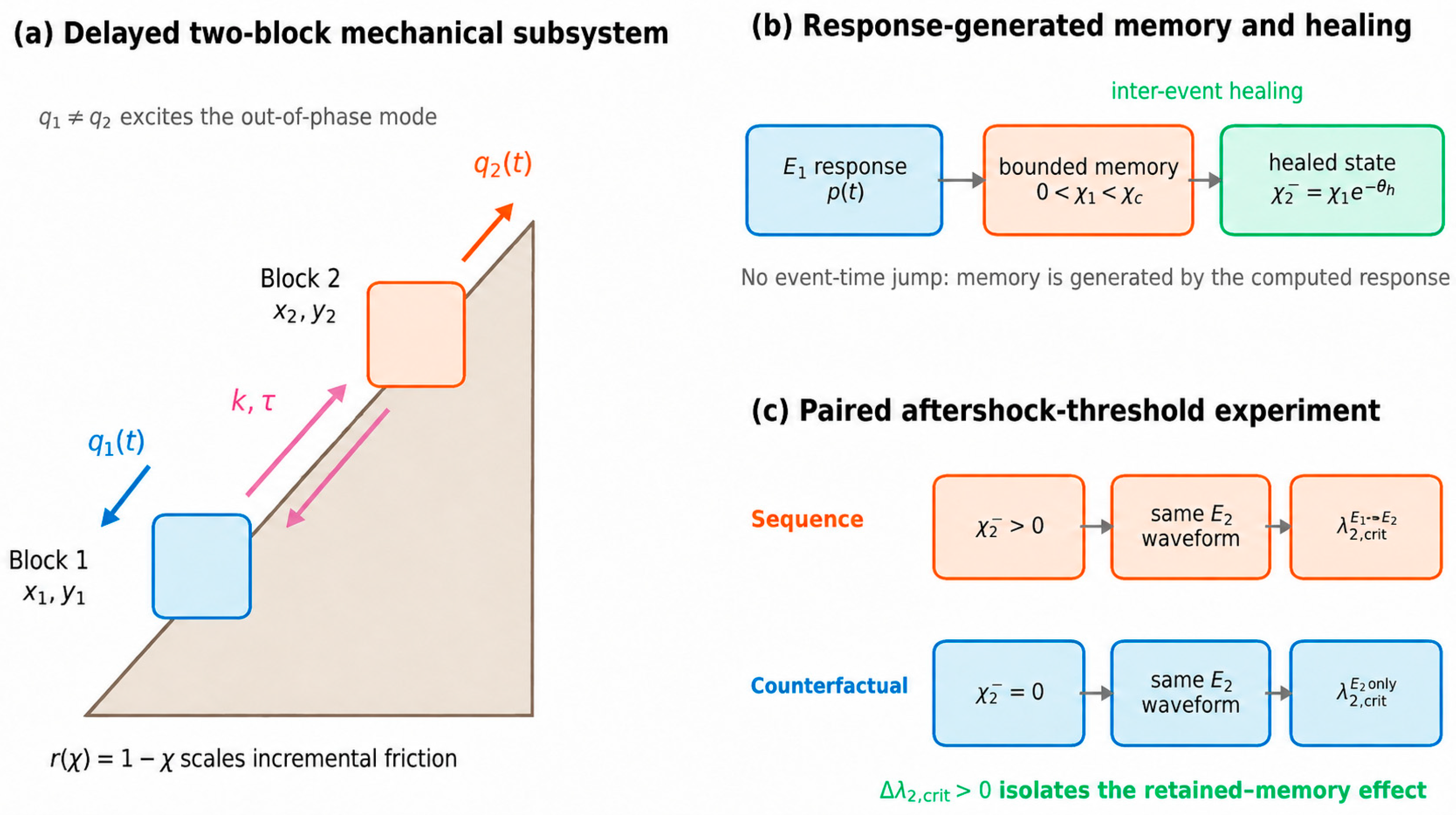
The causal structure of the model, the response-generated memory pathway, and the paired second-event counterfactual are summarised schematically in Figure 1.

2.2. Response-Generated Memory and Healing

The memory formulation is designed to satisfy three requirements essential for causal interpretation. First, memory must be generated exclusively by the computed mechanical response rather than by earthquake occurrence itself. Second, it must remain bounded so that susceptibility cannot grow without limit. Third, it must recover continuously between earthquakes, allowing transient rather than permanent preconditioning.

Accordingly, the slow state evolves as

$$\dot{\chi }={\alpha }_d\left(1-\chi \right)P\left(t\right)-{\displaystyle \frac{\chi }{T_h}}$$

(6)

where ${\alpha }_d$ is the damage-susceptibility coefficient, $T_h$ is the healing time, and

$$P\left(t\right)={\displaystyle \frac{1}{2}}{\displaystyle \sum _{i=1}^2}{\left[\Delta F_i\left(t\right)y_i\left(t\right)\right]}_{+}$$

(7)

$${\left[u\right]}_{+}=\mathrm{m}\mathrm{a}\mathrm{x}\left(u,0\right)$$

(8)

Here, P(t) denotes the non-negative dissipative-response measure that drives memory accumulation, while the positive-part operator ensures that only dissipative contributions can increase the memory state.

The positive-part operator admits only non-negative dissipative contributions, while the factor (1−χ) bounds the state below unity. Most importantly, no earthquake time, catalogue label, or peak ground acceleration (PGA) produces a discrete jump in χ. Every event enters only through q_i(t), modifies the fast mechanical response, and can change χ solely through the response-generated quantity P(t). Thus, the inherited state is an emergent dynamical coordinate rather than a prescribed damage increment.

In the present reduced-order formulation, χ is best interpreted as a normalised effective resistance-loss coordinate: its direct mechanical action is to scale the incremental frictional contribution through the factor 1 − χ. It is therefore not identified uniquely with excess pore-water pressure, crack density, cumulative shear strain, or a conventional scalar damage index. Instead, those quantities are possible material-level realisations of a common coarse-grained effect—temporary loss of effective resistance followed by recovery. Practical application would require a site- and material-specific observation operator, for example, χ = M(pw, Df, εp, …), constrained by pore-pressure, fracture, deformation, or stiffness measurements. The present study identifies the causal dynamical role of such an inherited state but does not calibrate that mapping.

When inter-event mechanical activity is negligible, the healing law has the analytical solution

$$\chi \left(t_2^{-}\right)=\chi \left(t_1^{+}\right)\mathrm{e}\mathrm{x}\mathrm{p}\left(-{\displaystyle \frac{\Delta t}{T_h}}\right)$$

(9)

This relation motivates three dimensionless coordinates used throughout the study:

$${\Theta }_h={\displaystyle \frac{\Delta t}{T_h}}$$

(10)

$${\rho }_1={\displaystyle \frac{\chi \left(t_{1,\mathrm{e}\mathrm{n}\mathrm{d}}+T_{\mathrm{d}\mathrm{y}\mathrm{n}}\right)}{{\chi }_c}}$$

(11)

$${\rho }_2^{-}={\rho }_1\mathrm{e}\mathrm{x}\mathrm{p}\left(-{\Theta }_h\right)$$

(12)

These quantities represent, respectively, the dimensionless healing interval, the post-first-event proximity to criticality, and the retained memory immediately before the second earthquake. Because they arise directly from the governing dynamics, they permit a comparison of identical external forcing applied to systems with different inherited susceptibility.

Regarding the applicability of the healing law, the single exponential recovery used here is a one-timescale closure selected to isolate the causal consequence of a continuously decaying inherited state. It is appropriate only when recovery over the interval of interest can be represented by one dominant effective timescale. Slopes in which rapid pore-pressure dissipation is followed by slower fracture closure, contact ageing, or fabric recovery may require two or more recovery timescales. A natural extension is a weighted multi-exponential or otherwise non-exponential healing law. No claim is made that the present exponential form is a universal constitutive law for postseismic healing.

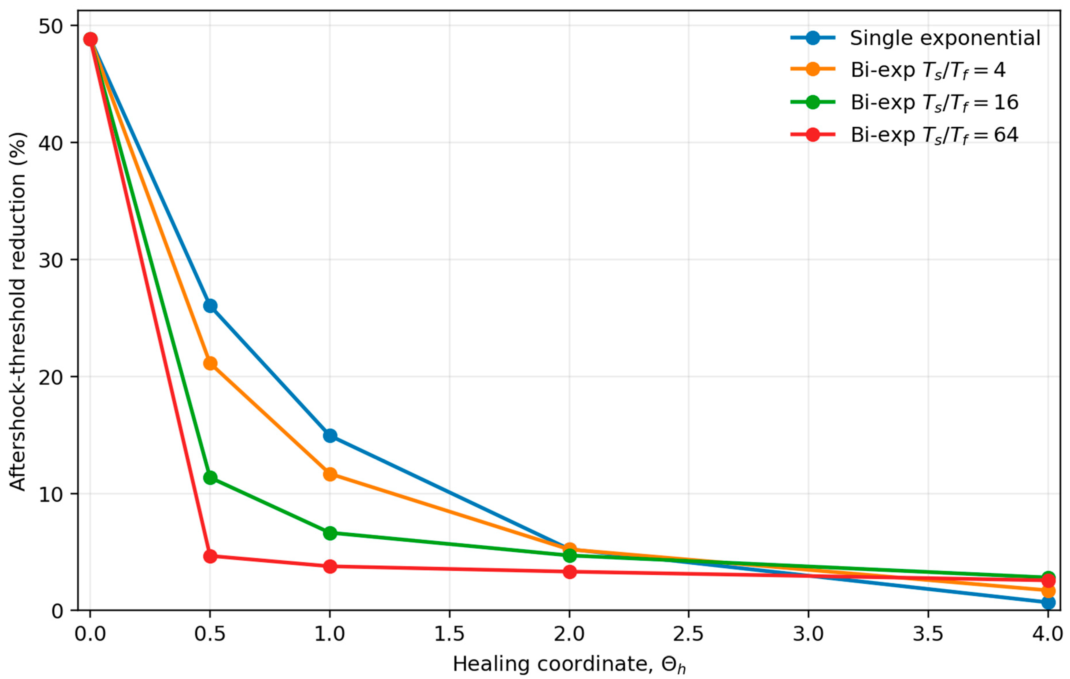
Also, to test whether the sequence effect depends qualitatively on the one-timescale closure, an auxiliary bi-exponential recovery law was evaluated while retaining the single-exponential law as the primary formulation. The reported post-first-event reference state ${\rho }_1=0.727720$ was held fixed so that only the inter-event retention map changed. The reference retention factor $h\left({\Theta }_h\right)=\mathrm{e}\mathrm{x}\mathrm{p}(-{\Theta }_h)$ was compared with $h({\Theta }_h)=w_f\mathrm{e}\mathrm{x}\mathrm{p}(-r{\Theta }_h)+w_s\mathrm{e}\mathrm{x}\mathrm{p}(-{\displaystyle \frac{{\Theta }_h}{r}})$, with $r=2,4,8,w_f={\displaystyle \frac{r}{r+1}},w_s={\displaystyle \frac{1}{r+1}}$ These choices give ${\displaystyle \frac{T_s}{T_f}}=4,16,64$ while preserving the weighted mean recovery time, $w_f{T}_f+w_s{T}_s=T_h$. The sensitivity therefore redistributes the same nominal healing timescale between a dominant fast component and a weaker slow component; no site-specific calibration of the auxiliary timescales is implied.

2.3. Objective Stability Boundary

A central requirement of the framework is that the critical memory level must not be introduced as an adjustable parameter. The activation boundary is therefore derived independently from the delayed mechanical subsystem before any earthquake-threshold experiment is performed. Subsequent simulations do not calibrate criticality; they determine how earthquake sequences move the system relative to an already established stability boundary.

With χ frozen, the tangent friction coefficient is

$$c_V=F^{\prime }\left(V\right)=3a{V}^2-2bV+c$$

(13)

Transformation into in-phase and out-of-phase modal coordinates yields the characteristic equations

$$p_{\mathrm{i}\mathrm{n}}\left(s;\chi \right)=s^2+\left(1-\chi \right)c_{V}s+k\left(1-e^{-s\tau }\right)=0$$

(14)

$$p_{\mathrm{o}\mathrm{u}\mathrm{t}}\left(s;\chi \right)=s^2+\left(1-\chi \right)c_{V}s+k\left(1+e^{-s\tau }\right)=0$$

(15)

The neutral translation root s = 0 in the in-phase mode is excluded because it represents rigid translation rather than mechanical instability. The critical state is defined as

$${\chi }_c=\mathrm{i}\mathrm{n}\mathrm{f}\left\{\chi \in [0,1):\mathrm{m}\mathrm{a}\mathrm{x}\mathrm{R}\mathrm{e}\left(s\right)\ge 0\right\}$$

(16)

where the maximum is evaluated over all non-neutral roots of both characteristic equations. If the first crossing is oscillatory with critical root $s_c$, the corresponding intrinsic dynamical time is

$$T_{\mathrm{d}\mathrm{y}\mathrm{n}}={\displaystyle \frac{2\pi }{\left|\mathrm{I}\mathrm{m}\left(s_c\right)\right|}}$$

(17)

This timescale provides the common reference for healing, noise correlation, burn-in duration, and persistence testing.

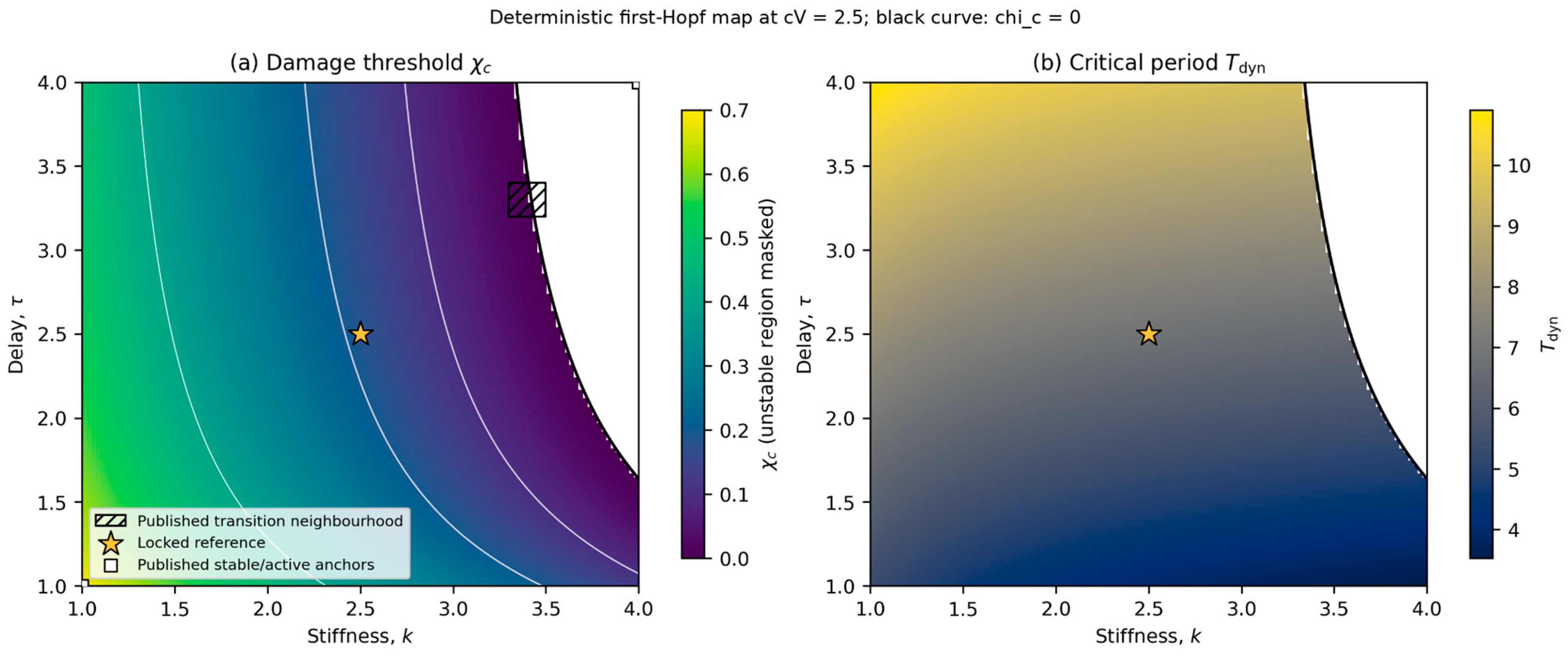
The source article did not report the numerical value of V. Rather than introducing an additional fitted parameter, the tangent-friction target was reconstructed from the published transition neighbourhood, 3.3 ≤ k ≤ 3.5 and 3.2 ≤ τ ≤ 3.4, which gives 2.445 ≤ F′(V) ≤ 2.536. The rounded midpoint F′(V) = 2.5 was adopted as the reference target. Solving this relation gives V = 0.18174 on the low-velocity creep branch used in the primary analysis and V = 1.31826 on the high branch retained for nonlinear sensitivity. Additional digits are retained only in the computational files and are not interpreted as physical accuracy.

At the locked reference k = τ = 2.5, the independently derived boundary is

$${\chi }_c=0.18445$$

(18)

$${\omega }_c=0.91814$$

(19)

$$T_{\mathrm{d}\mathrm{y}\mathrm{n}}=6.84337$$

(20)

The first loss of stability is an out-of-phase Hopf mode. The secondary in-phase crossing occurs at χ = 0.45756. These rounded values are sufficient for interpretation in the main manuscript; the calculations retain full internal floating-point precision. The stability quantities are therefore reported as dynamical characteristics of the reference model rather than as independently measured site parameters.

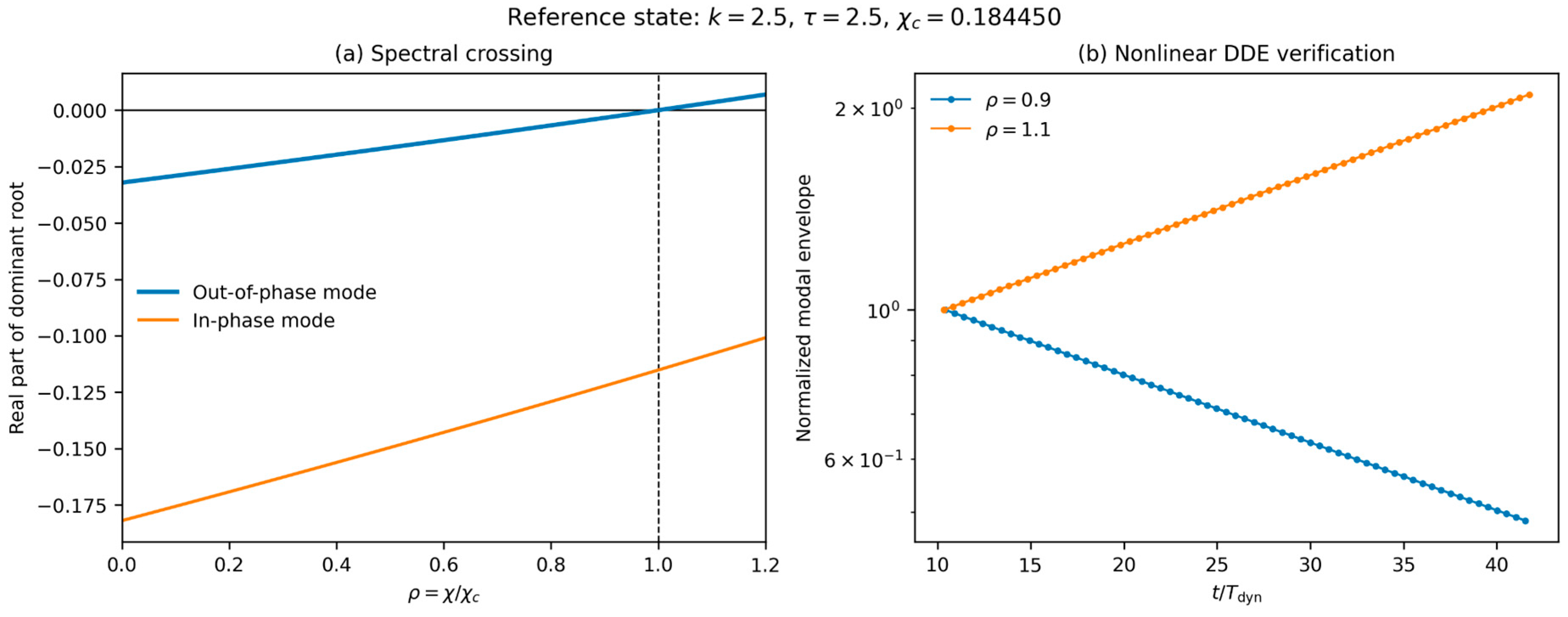
Figure 2 maps the critical memory state and the corresponding critical period over stiffness-delay space, while Figure 3 verifies the locked reference boundary by both characteristic-root crossing and direct nonlinear delayed simulation.

• Physical Interpretation of Delay and Time Mapping

The delay τ is an effective interaction delay in the reduced-order mechanical subsystem. It represents unresolved finite-time transmission and redistribution between neighbouring slope elements rather than a uniquely assigned physical process. Depending on the slope and failure mechanism, possible contributors include stress redistribution along a shear zone, progressive contact mobilisation, finite wave-mediated interaction, and hydro-mechanical lag. The present formulation does not decompose these contributions and therefore does not identify τ with a seismic travel time or a pore-pressure diffusion time.

Likewise, γt maps recorded physical time to model time and is deliberately treated as an unresolved coordinate. The reference γt = 1 is not a statement that one model-time unit equals one second. Consequently, the Hopf analysis establishes the existence and robustness of a delay-induced instability in dimensionless parameter space, but it does not by itself demonstrate that a particular natural slope occupies the corresponding physical delay range. Engineering use requires the independent calibration of γt and τ from monitoring or wave-propagation/deformation data before Tdyn or the Hopf boundary can be expressed in seconds.

2.4. Physically Documented Earthquake Forcing

The forcing protocol is designed for mechanism identification rather than site-specific calibration. Recorded ground motions provide physically documented excitation histories, while all transfer coefficients connecting the recordings to the reduced-order model remain explicit model parameters rather than fitted site properties.

For event e, the east–north–up acceleration vector is

$${\mathbf{a}}^{\left(e\right)}=\left(a_E^{\left(e\right)},a_N^{\left(e\right)},a_U^{\left(e\right)}\right)$$

(21)

For slope aspect A, measured clockwise from north, and dip β, the downslope unit vector is

$$\mathbf{s}\left(A,\beta \right)=\left(\mathrm{s}\mathrm{i}\mathrm{n}A\mathrm{c}\mathrm{o}\mathrm{s}\beta ,|\mathrm{c}\mathrm{o}\mathrm{s}A\mathrm{c}\mathrm{o}\mathrm{s}\beta ,|-\mathrm{s}\mathrm{i}\mathrm{n}\beta \right)$$

(22)

The projected downslope acceleration is

$$a_{\parallel }^{\left(e\right)}\left(t;A,\beta \right)={\mathbf{a}}^{\left(e\right)}\left(t\right)\cdot \mathbf{s}\left(A,\beta \right)$$

(23)

and the forcing of block i is

$$q_i\left(t\right)=-{\lambda }_1{\displaystyle \frac{a_{\parallel ,i}^{\left(1\right)}\left(t-t_1\right)}{g}}-{\lambda }_2{\displaystyle \frac{a_{\parallel ,i}^{\left(2\right)}\left(t-t_2\right)}{g}}$$

(24)

The multipliers ${\lambda }_1$ and ${\lambda }_2$ absorb the unresolved mapping between recorded acceleration and dimensionless local block forcing. The waveforms are not normalised event by event; their recorded relative amplitudes, durations, and frequency contents are retained in every comparison.

The primary documented pair comprises the February 2011 Christchurch earthquake (GeoNet event 3468575; M_w = 6.2; 21 February 2011 23:51:42 UTC) and the June 2011 Christchurch earthquake (GeoNet event 3528839; M_w = 6.0; 13 June 2011 02:20:49 UTC). Both belong to the 2010–2011 Canterbury earthquake sequence in New Zealand. Their separation is 9,599,347 s, or 111.104 d. Corrected Vol2 records from station HVSC were obtained from the GeoNet Strong Motion Data Products dataset [36]. The files 20110221_235142_HVSC.V2A and 20110613_022049_HVSC.V2A are both sampled at 0.02 s.

The two blocks use projections corresponding to the northeast and southeast Redcliffs faces:

$$\left(A_1,{\beta }_1\right)=\left({54}^{\circ },{67}^{\circ }\right)$$

(25)

$$\left(A_2,{\beta }_2\right)=\left({132}^{\circ },{67}^{\circ }\right)$$

(26)

Their common and differential inputs are

$$q_c={\displaystyle \frac{q_1+q_2}{2}}$$

(27)

$$q_d={\displaystyle \frac{q_1-q_2}{2}}$$

(28)

$$q_1\left(\eta \right)=q_c+\eta q_d, q_2\left(\eta \right)=q_c-\eta q_d$$

(29)

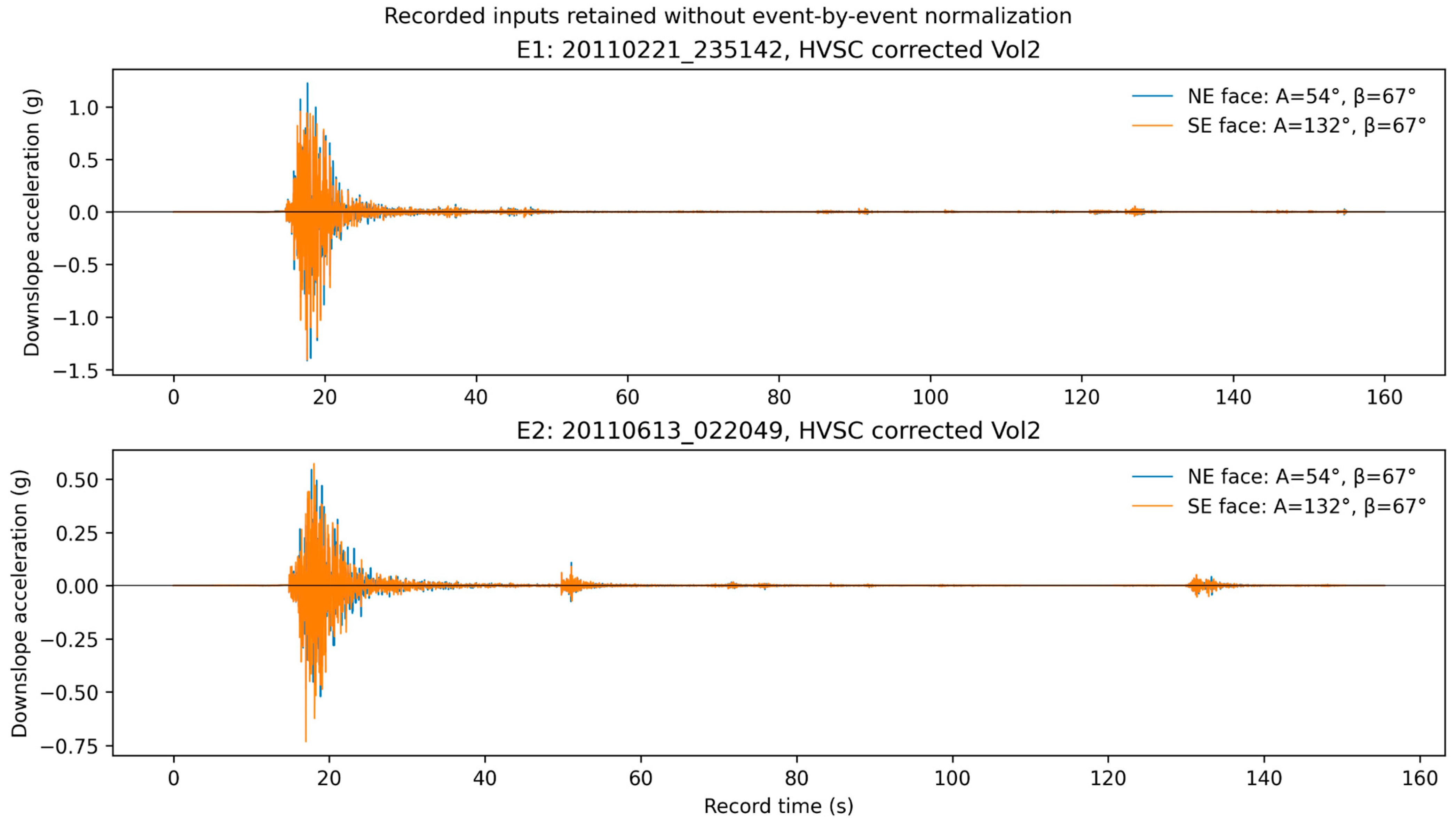
Here, $\eta =1$ is the geometry-derived projection, $\eta =0$ is the exact common-input control, and other values are sensitivity coordinates rather than fitted site parameters. The projected peak accelerations are 1.41580 g and 1.40454 g for $E_1$, and 0.54497 g and 0.73216 g for $E_2$, on the northeast and southeast faces, respectively.

The corresponding projected acceleration histories are shown in Figure 4, which demonstrates that the recorded relative amplitudes and frequency content are retained without event-wise normalisation.

For an auxiliary cross-pair robustness check, the September 2010 Darfield earthquake was additionally used as a first event before the February 2011 Christchurch event. The corrected HVSC record 20100903_163541_HVSC.V2A is sampled at 0.02 s and identifies the Darfield event as Mw 7.2 at 3 September 2010 16:35:41 UTC. Projection onto the same northeast and southeast Redcliffs faces gives absolute peak downslope accelerations of 0.27834 g and 0.28867 g, respectively. The physical interval from Darfield to the February event is 14,800,561 s, or 171.303 d. This additional pair is used only as a within-Canterbury robustness check; the February–June 2011 pair remains the primary experiment.

Descriptive statistics of all projected corrected records used in the primary and auxiliary calculations are provided in Appendix F,

Table A4. Descriptive statistics of the projected corrected accelerograms used in the primary and auxiliary calculations. Acceleration values are in g; means are near zero because the Vol2 records are corrected strong-motion products.

Event	Face	N	Duration (s)	Min (g)	Max (g)	Mean (g)	SD (g)	PGA |g|
Darfield 2010	NE	7431	148.60	−0.240921	0.278338	−6.50 × 10−8	0.024890	0.278338
Darfield 2010	SE	7431	148.60	−0.247329	0.288673	−3.48 × 10−8	0.025211	0.288673
February 2011	NE	8000	159.98	−1.415801	1.225767	−4.22 × 10−8	0.077541	1.415801
February 2011	SE	8000	159.98	−1.404536	0.954448	−4.82 × 10−8	0.076961	1.404536
June 2011	NE	7773	155.44	−0.521918	0.544969	6.25 × 10−8	0.037321	0.544969
June 2011	SE	7773	155.44	−0.732161	0.573082	6.26 × 10−8	0.040782	0.732161

Note. NE and SE denote the northeast and southeast Redcliffs face projections. The February and June 2011 records define the primary experiment; Darfield 2010 is used only in the auxiliary within-Canterbury robustness check. No event-wise normalisation was applied.

. The table reports record length, duration, minimum, maximum, mean, standard deviation, and peak absolute acceleration for each Redcliffs projection. These statistics characterise the recorded forcing histories; they are not used to calibrate the mechanical model.

The delayed mechanical, memory/healing, stability, threshold, and stochastic equations are solved in nondimensional model variables. Equations (21)–(30) provide the explicit interface from the recorded physical accelerograms to those model coordinates: the acceleration histories retain their measured amplitudes before the declared transfer mapping, while physical record time is mapped to model time according to

$$t_{\mathrm{m}\mathrm{o}\mathrm{d}\mathrm{e}\mathrm{l}}={\gamma }_t{t}_{\mathrm{r}\mathrm{e}\mathrm{c}\mathrm{o}\mathrm{r}\mathrm{d}}$$

(30)

The choice ${\gamma }_t$ = 1 is only a transparent reference convention. It does not assert physical equality between one model time unit and one second; ${\gamma }_t$ is swept as a primary phase coordinate.

2.5. Experimental Design

The experiments isolate the causal contribution of retained memory while holding the second-earthquake waveform and all model coordinates fixed. The only permitted difference between the sequence and second-event-only arms is the inherited state generated by the non-activating first earthquake. Deterministic simulations establish the threshold structure without background variability, whereas stochastic simulations test whether the same mechanism remains detectable under random excitation.

2.5.1. Deterministic Experiments

The deterministic phase map used

$${\alpha }_d\in \left\{8,8\sqrt{2},16,16\sqrt{2},32,32\sqrt{2}\right\}$$

(31)

$${\gamma }_t=0.5\hspace{0.17em}{2}^{j/4}, j=0,\dots ,8$$

(32)

$$\eta \in \left\{0,0.03,0.1,0.3,1,2\right\}$$

(33)

$${\Theta }_h\in \left\{0,0.5,1,2,4\right\}$$

(34)

The first-event multiplier was fixed at ${\lambda }_1$ = 1. A parameter cell entered the paired comparison only if $E_1$ caused no persistent stability loss and generated a non-zero but subcritical state, 0 < ${\rho }_1$ < 1. Cells violating these requirements were classified as first-event-critical and excluded from interpretation as second-event-triggered activation.

For each admissible state and healing level, the $E_2$-only threshold, ${\lambda }_{2,crit}^{E_2 only}$, and the sequence threshold, ${\lambda }_{2,crit}^{E_1\to E_2}$, were recomputed at identical ${\alpha }_d$, ${\gamma }_t$, and $\eta$.

For each threshold search, the second-event multiplier was increased until an inactive and an active solution bracketed the transition. The adaptive search was allowed to extend to 64 if necessary, after which the bracket was refined by 12 bisection iterations. Threshold reduction was defined as

$$R_{\lambda }=100\left[1-{\displaystyle \frac{{\lambda }_{2,\mathrm{c}\mathrm{r}\mathrm{i}\mathrm{t}}^{E_1\to E_2}}{{\lambda }_{2,\mathrm{c}\mathrm{r}\mathrm{i}\mathrm{t}}^{E_2\hspace{0.17em}\mathrm{o}\mathrm{n}\mathrm{l}\mathrm{y}}}}\right]$$

(35)

Severity metrics were evaluated at ${\lambda }_{2probe}$ = 1.05 ${\lambda }_{2upper}$, while threshold crossing and realised antisymmetric amplitude were retained as distinct outputs.

Regarding the local friction-law sensitivity, a one-at-a-time local constitutive sensitivity was evaluated around the inherited reference coefficients a = 3.2, b = 7.2, and c = 4.8. Each coefficient was independently perturbed by ±2.5%, with the remaining two retained at their reference values. For every perturbed parameter set, the tangent friction coefficient and characteristic-root stability boundary were recomputed before earthquake forcing; consequently, for χ_c, the critical Hopf properties, ρ₁, and ρ₂⁻ were scenario-specific. The same recorded inputs, geometry, α_d, γ_t, η, and healing coordinate were then retained. These perturbations are local robustness coordinates and are not interpreted as calibrated ranges for particular geomaterials.

As for the robustness check, the Darfield–February calculation used the same reference mechanical coordinates, geometry, λ₁ = 1, activation criterion, adaptive threshold bracketing, and 12 bisection iterations as the primary deterministic experiment. First-event admissibility was verified before the February threshold comparison. To preserve the effective healing time implicit in the primary reference calculation, Θh = 0.5 over the 111.103553 d February–June interval was mapped to Θh = 0.770915 over the 171.302789 d Darfield–February interval. A second control retained Θh = 0.5 directly, separating the waveform/pair change from the longer physical interval.

2.5.2. Stochastic Experiments

Three forcing conditions were compared. The deterministic condition has dNi = 0. White noise is represented by

$$d{N}_i=\sqrt{2D}\hspace{0.17em}d{W}_i$$

(36)

whereas Ornstein–Uhlenbeck forcing is

$$d{N}_i=z_i\hspace{0.17em}dt$$

(37)

$$d{z}_i=-{\displaystyle \frac{z_i}{{\tau }_c}}\hspace{0.17em}dt+{\displaystyle \frac{\sqrt{2D}}{{\tau }_c}}\hspace{0.17em}d{W}_i$$

(38)

This normalisation converges to the declared white-noise model as τ_c→ 0, so D denotes the same long-time diffusion intensity in both conditions. Correlation time is expressed relative to the intrinsic delayed-system period as

$${\Theta }_c={\displaystyle \frac{{\tau }_c}{T_{\mathrm{d}\mathrm{y}\mathrm{n}}}}.$$

(39)

The stochastic forcing forms are adopted from the previous random- and coloured-noise delay-model formulations [29,30], whereas the integrated-intensity normalisation, paired common-random-number design, and activation-threshold protocol are specified here for the present sequence experiment.

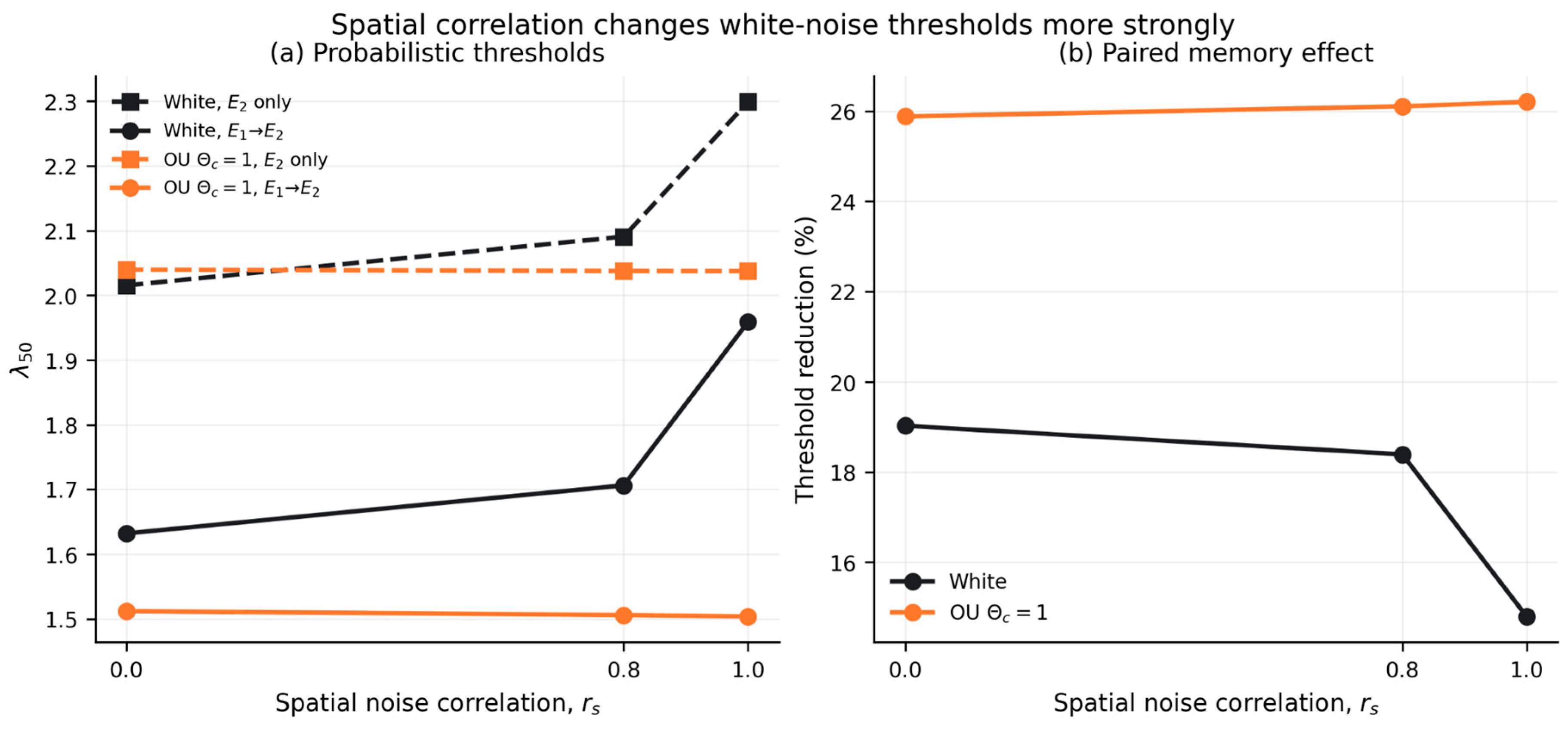
The fixed OU grid was ${\Theta }_c$ ∈ {0.05, 0.25, 1, 4}. Primary block noises were independent ($r_s=0$), while $r_s=0$.8 and $r_s=1$ were tested as spatial-correlation sensitivities.

Regarding the physical interpretation of the stochastic terms, the white-noise condition represents unresolved broadband disturbances whose correlation time is short relative to Tdyn, such as weak microseismicity, high-frequency environmental vibration, or local anthropogenic disturbance after coarse graining. OU forcing represents temporally correlated background perturbations: Θc ≪ 1 corresponds to short-memory fluctuations, Θc ≈ 1 to forcing whose persistence competes directly with the critical delayed mode, and Θc ≫ 1 to slowly varying forcing relative to the mechanical response. These are dynamical timescale classes rather than one-to-one labels for specific field processes. In particular, rainfall is not treated here as a direct random mechanical force; in a physically coupled model, it would more naturally enter through hydraulic state variables that modify resistance, effective stress, and healing.

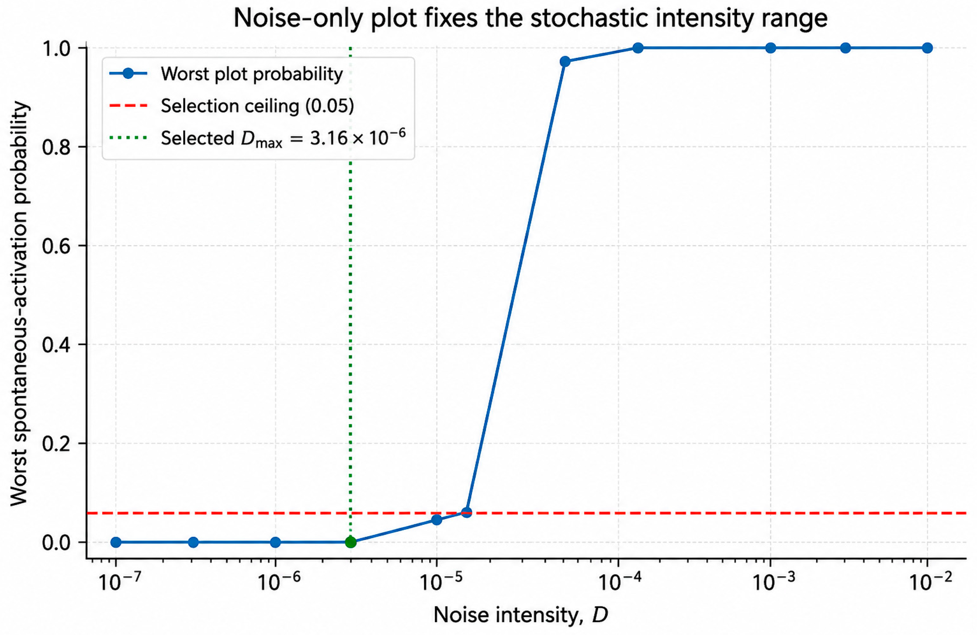
A 256-realisation no-earthquake pilot fixed D_max = 3.162 × 10⁻⁶ and the primary intensities D ∈ {1.976 × 10⁻⁷, 7.906 × 10⁻⁷, 3.162 × 10⁻⁶}. The next candidate, D = 10⁻⁵, was excluded because the worst spontaneous-control probability exceeded 0.05. No earthquake outcome was used to choose this range.

The stochastic differential equations were integrated by stochastic Heun with Δt = τ/1000 = 0.0025. Memory accumulation was disabled during burn-in and reset to the scenario-specific value at the start of the event window. Burn-in lasted 10$T_{\mathrm{d}\mathrm{y}\mathrm{n}}$ for white noise and max(10$T_{\mathrm{d}\mathrm{y}\mathrm{n}}$, 5${\tau }_c$) for OU noise. Background noise acted during burn-in, the recorded-event window, and post-event ringdown; the 111-day inter-event gap was represented analytically by the healing map rather than by continuous stochastic integration.

Primary no-event controls contained 1024 realisations, and primary event ensembles contained 512 realisations at each ${\lambda }_2$. Selected confirmation cells contained 4096 realisations per arm. Paired comparisons used identical Wiener paths. After preliminary coarse estimates were discarded, both arms were symmetrically refined until the isotonic $P_{\mathrm{a}\mathrm{c}\mathrm{t}}$ = 0.5 bracket was no wider than 1% of the deterministic $E_2$-only threshold. Common random numbers reduce Monte Carlo variance while preserving the paired causal comparison.

2.6. Activation Criterion and Statistical Inference

The activation criterion is designed to distinguish persistent delayed instability from brief threshold crossings, transient oscillation, and stochastic background motion. Let Lc denote the longest uninterrupted duration for which χ(t) ≥ χc. Persistent stability loss requires

$$L_c\ge T_{\mathrm{d}\mathrm{y}\mathrm{n}}$$

(40)

Mechanical persistence after $E_2$ is evaluated using residual kinetic activity,

$$V_{\mathrm{p}\mathrm{o}\mathrm{s}\mathrm{t}}={\left[{\displaystyle \frac{1}{4T_{\mathrm{d}\mathrm{y}\mathrm{n}}}}{\int }_{t_{2,\mathrm{e}\mathrm{n}\mathrm{d}}+T_{\mathrm{d}\mathrm{y}\mathrm{n}}}^{t_{2,\mathrm{e}\mathrm{n}\mathrm{d}}+3T_{\mathrm{d}\mathrm{y}\mathrm{n}}}{\displaystyle \sum _{i=1}^2}{y}_i^2\left(t\right)\hspace{0.17em}dt\right]}^{1/2}$$

(41)

and residual mean displacement,

$$\Delta X_{\mathrm{r}\mathrm{e}\mathrm{s}}=\bar{x}\left(t_{2,\mathrm{e}\mathrm{n}\mathrm{d}}+3T_{\mathrm{d}\mathrm{y}\mathrm{n}}\right)-\bar{x}\left(t_{2,\mathrm{e}\mathrm{n}\mathrm{d}}\right)$$

(42)

$$\bar{x}={\displaystyle \frac{x_1+x_2}{2}}$$

(43)

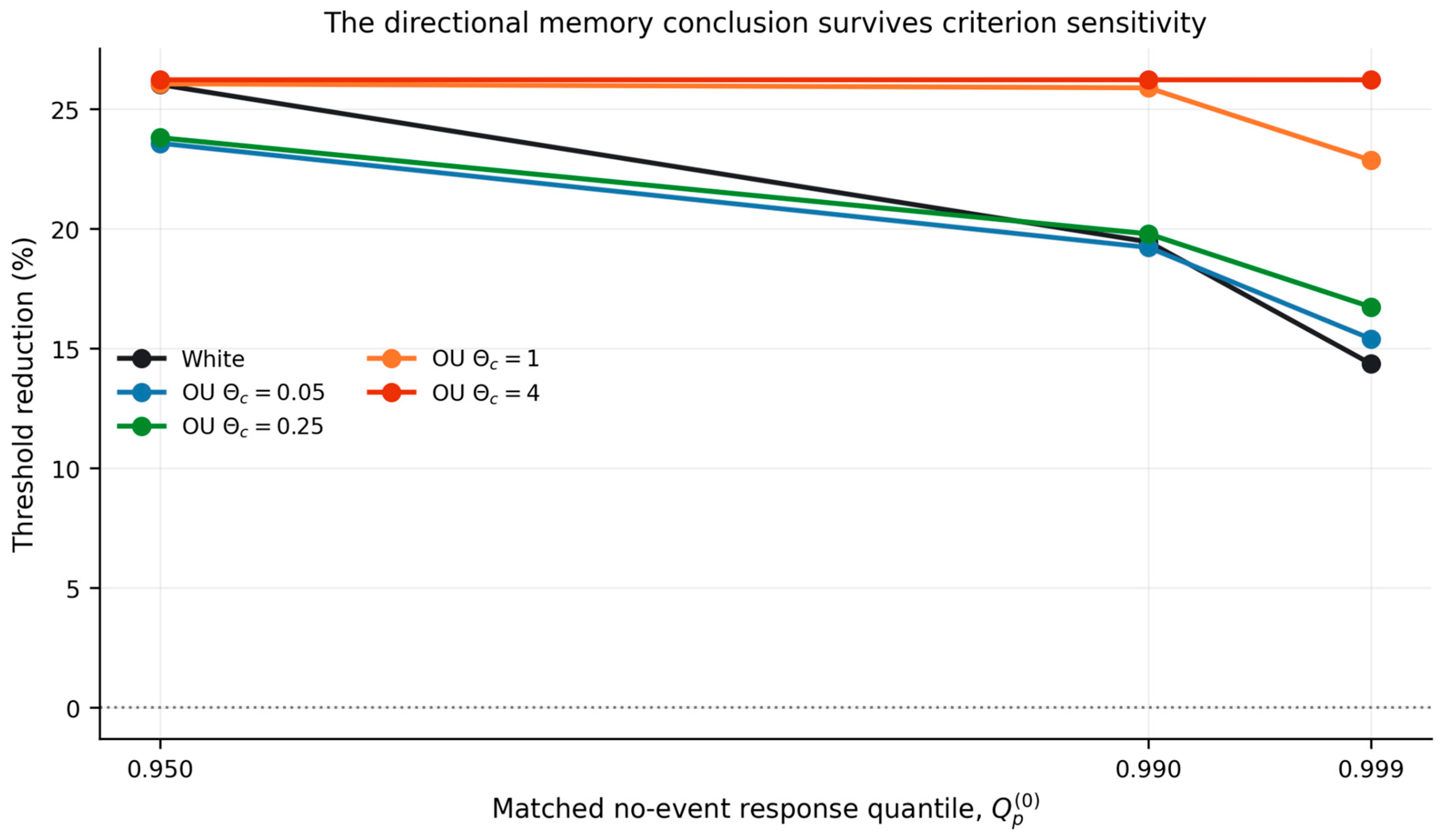
For each noise condition, matched no-earthquake ensembles define the 99th-percentile reference values $Q_{0.99}^{\left(0\right)}$. The binary activation indicator Y = 1 requires both persistent stability loss and either $V_{\mathrm{p}\mathrm{o}\mathrm{s}\mathrm{t}}$ > $Q_{0.99}^{\left(0\right)}$($V_{\mathrm{p}\mathrm{o}\mathrm{s}\mathrm{t}}$) or $\Delta X_{\mathrm{r}\mathrm{e}\mathrm{s}}$ > $Q_{0.99}^{\left(0\right)}$($\Delta X_{\mathrm{r}\mathrm{e}\mathrm{s}}$). The 0.95 and 0.999 percentiles are retained as sensitivity checks.

This criterion intentionally distinguishes mathematical activation of the reduced-order model from physical landslide failure. It identifies persistent dynamically sustained motion beyond the range expected from background fluctuations alone.

Accordingly, Lc ≥ Tdyn is not, by itself, the activation criterion. It is only the persistent-boundary-crossing requirement. Model activation additionally requires post-event residual kinetic activity or residual mean displacement to exceed the corresponding matched no-earthquake reference level. Even this combined criterion remains a reduced-order dynamical indicator rather than a prediction of physical slope failure. Permanent residual displacement in metres, cumulative shear strain within a localised shear band, excess pore-water pressure, and failed volume would require additional constitutive and geometric mappings that are outside the present mechanism-identification study.

The stochastic threshold ${\lambda }_{50}$ satisfies

$$\mathrm{P}\mathrm{r}\left(Y=1\mid {\lambda }_2={\lambda }_{50}\right)=0.5$$

(44)

Paired bootstrap intervals preserve the common-random-number structure. The sequence estimand is conditional on $E_1$ not activating.

For the deterministic dependence analysis, Spearman’s rank coefficient was calculated over all 1255 admissible paired comparisons by ranking the retained pre-second-event state ρ₂⁻ and the corresponding relative threshold reduction, using average ranks for ties, and evaluating the ordinary Pearson correlation between the two rank vectors. This gives ρS = 0.9997. A conventional two-sided null test gives an effectively vanishing p-value (p ≪ 10⁻³⁰⁰). Because the 1255 points form a structured deterministic parameter grid rather than independent random observations from a population, this p-value is reported only as a conventional measure of association strength; the physically relevant result is the near-unity monotonic rank relation across the admissible domain.

2.7. Causal Controls and Numerical Verification

The principal mechanism is challenged by controls that remove, one at a time, the components required for the proposed causal interpretation. Resetting memory immediately before $E_2$ tests whether inheritance is necessary. Setting $\tau =0$ tests whether retained susceptibility alone is sufficient or whether activation requires delayed instability. No-earthquake simulations establish spontaneous-activation rates and response percentiles. Exact common forcing ($\eta =0$), combined with fully correlated block noise, suppresses differential excitation and separates latent boundary crossing from the realisation of the antisymmetric mode.

Deterministic fourth-order Runge–Kutta (RK4) simulations with delayed-history interpolation were independently checked against a compiled implementation. The stochastic engine was compared with the deterministic solver, repeated-lambda random streams were checked for bitwise identity, and selected stochastic cells were recomputed at

$$\Delta t\in \left\{{\displaystyle \frac{\tau }{500}},{\displaystyle \frac{\tau }{1000}},{\displaystyle \frac{\tau }{2000}}\right\}$$

(45)

Together, the activation criterion, counterfactual controls, and independent numerical checks establish that measured threshold reductions arise from the interaction between response-generated memory and delayed mechanical instability rather than from numerical artefacts, stochastic variability, or prescribed event-dependent damage.

For reference,

Table 1. Principal parameters, roles, and calibration status.

Quantity	Primary Value or Grid	Role and Status
N	2	Number of blocks; fixed
a, b, c	3.2, 7.2, 4.8	Cubic friction; inherited
k, τ	2.5, 2.5	Reference coupling and delay; fixed before earthquake tests
V	0.18174	Low-velocity creep branch; high branch tested
χc	0.18445	Derived characteristic-root boundary
Tdyn	6.84337	Period of critical out-of-phase mode
αd	8 to 32√2	Swept susceptibility; not site-fitted
Θh	0, 0.5, 1, 2, 4	Dimensionless healing interval
γt	0.5 to 2, quarter-octaves	Record-to-model time mapping; unresolved
η	0 to 2	Differential input scale; $\eta =1$ geometry-derived
D	1.976 × ${10}^{-7}$ to 3.162 × ${10}^{-6}$	Noise intensity selected by no-event pilot
Θc	0.05, 0.25, 1, 4	OU correlation time relative to $T_{\mathrm{d}\mathrm{y}\mathrm{n}}$
λ1	1	First-event transfer convention
λ2	Adaptive	Second-event multiplier and threshold coordinate

summarises the principal model parameters and their calibration status, whereas

Table 2. Experimental contrasts and their identifying roles.

Contrast	Inherited State at ${\mathit{E}}_2$	Identifying Purpose
$E_2$ only	χ2− = 0	Single-event counterfactual
$E_1\to E_2$, full model	χ2− > 0	Two-event effect
Memory reset	0	Tests whether inheritance is necessary
No delay	Scenario-specific χ2−	Tests whether boundary crossing requires delayed instability
No earthquake	Noise-generated only	Defines response percentiles and false-activation rate
Exact common mode	Scenario-specific χ2−	Separates latent crossing from antisymmetric-mode realisation

lists the experimental contrasts and the specific causal role of each control.

3. Results

3.1. The Delayed System Exhibits a Memory-Dependent Hopf Boundary

At $\chi =0$, the dominant antisymmetric eigenvalue pair is

$$-0.03212\pm 0.88723i$$

(46)

confirming that the reference state is linearly stable. As $\chi$ increases, the associated reduction in incremental friction moves this pair progressively toward the imaginary axis. The pair crosses the stability boundary at

$${\chi }_{\mathrm{c}}=0.18445$$

(47)

whereas the dominant symmetric pair retains a negative real part. The first instability is therefore associated with the antisymmetric mode.

Direct simulations of the delayed system confirmed the spectral prediction. Responses at

$$\rho ={\displaystyle \frac{\chi }{{\chi }_{\mathrm{c}}}}=0.9$$

(48)

decayed, whereas those at $\rho =1.1$ grew. At a time step of $\Delta t={\displaystyle \frac{\tau }{1000}}$, the fitted numerical growth rates differed from the characteristic-root predictions by less than $1.3\times {10}^{-7}$.

The robustness grid

$$2.25\le k,\tau \le 2.75,2.3\le c_{\mathrm{V}}\le 2.7$$

(49)

contained 27 parameter combinations. All 27 states were stable, and the antisymmetric mode remained the first mode to lose stability in every case. Across this grid, they ranged from 0.0526 to 0.3018, whereas the characteristic dynamical period ranged from 6.262 to 7.439. The identified instability mechanism is therefore robust within the local parameter neighbourhood and is not a single-point bifurcation artefact.

3.2. The Mainshock Defines the Admissible Preconditioning Domain

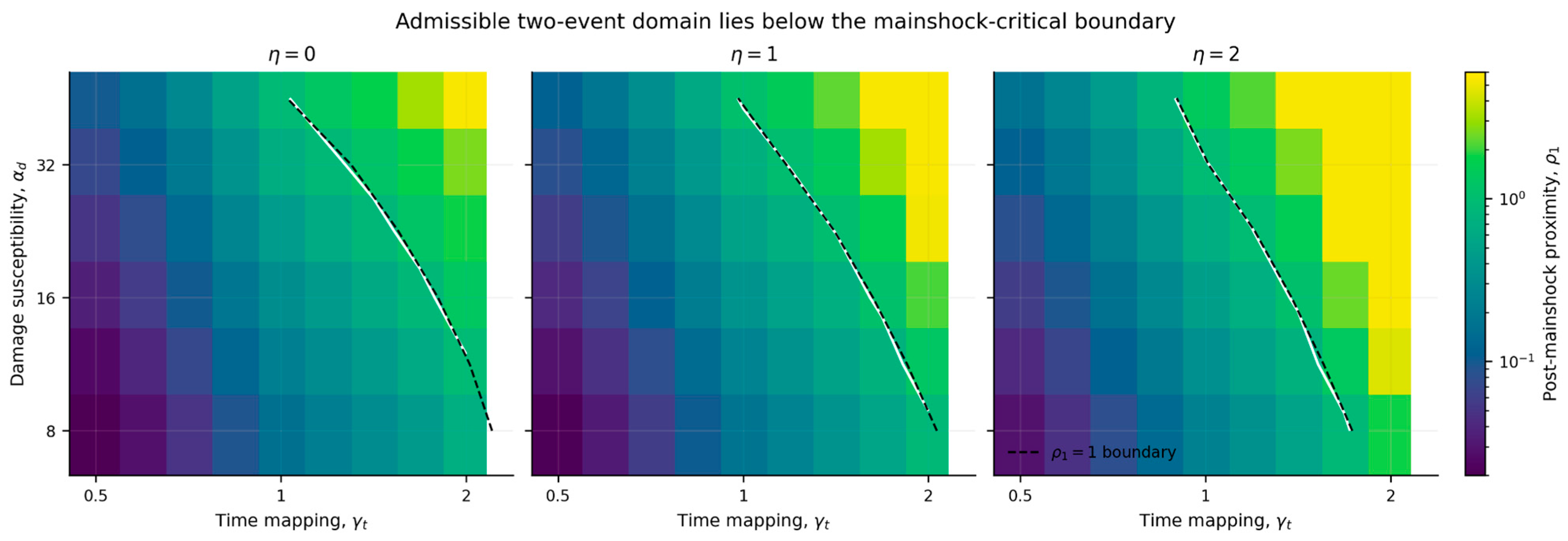
Of the 324 deterministic mainshock simulations, 251 remained non-activating and satisfied

$$0<{\rho }_1<1$$

(50)

Their post-mainshock states covered the interval

$$0.0177\le {\rho }_1\le 0.9804$$

(51)

The remaining 73 simulations reached the mainshock-critical condition and were excluded from the aftershock-triggered estimand. This exclusion ensures that all subsequent comparisons concern sequences in which $E_1$ modifies the inherited state without itself activating the model.

The admissible domain contracted as increased because the recorded ground motion then occupied a longer interval in model time. At the geometry-derived differential forcing level, the continuous-critical value decreased from 2.065 at to 0.981 at

$${\alpha }_{\mathrm{d}}=32\surd 2$$

(52)

Differential projection also shifted the admissibility boundary relative to exact common forcing. These results show that a two-event interpretation requires an explicit verification that the first earthquake remains subcritical. Apparent threshold reductions outside this domain cannot be attributed to preconditioning by a non-activating $E_1$.

Figure 5 visualises this admissible preconditioning domain and shows how the first-event-critical boundary changes with the differential projection scale.

3.3. Retained Memory Lowers the Deterministic Aftershock Threshold

The 251 admissible mainshock states generated 1255 paired threshold comparisons across five healing levels. Every midpoint estimate satisfied

$${\lambda }_{2,\mathrm{c}\mathrm{r}\mathrm{i}\mathrm{t}}^{({\mathrm{E}}_1\to {\mathrm{E}}_2)}<{\lambda }_{2,\mathrm{c}\mathrm{r}\mathrm{i}\mathrm{t}}^{\left({\mathrm{E}}_2\mathrm{o}\mathrm{n}\mathrm{l}\mathrm{y}\right)}$$

(53)

The numerical threshold intervals were strictly separated in 1235 comparisons. The remaining 20 unresolved intervals all occurred at ${\Theta }_{\mathrm{h}}=4$, where the estimated reductions were only 0.014–0.022% and the retained pre-aftershock states were

$$0.00032\le {\rho }_2^{-}\le 0.00074$$

(54)

These cases represent numerical convergence toward the aftershock-only healing limit rather than resolved evidence of a persistent threshold difference.

Across the full admissible domain, the relative threshold reduction $R_{\mathsf{\lambda }}$ ranged from 0.014% to 86.305%. The largest values occurred as ${\rho }_1\to 1^{-}$ and therefore correspond to near-critical model states rather than site-specific estimates.

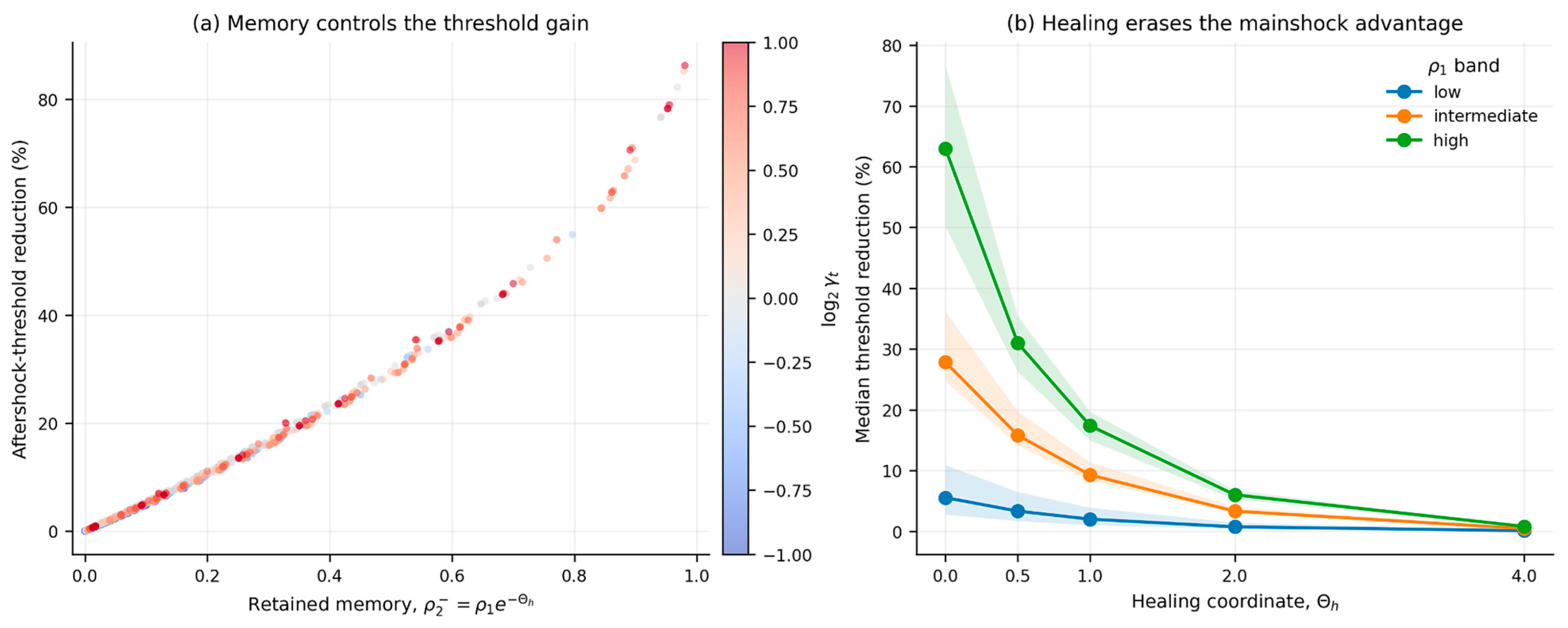
Retained memory accounted for almost all rank variation in threshold reduction:

$$\mathrm{S}\mathrm{p}\mathrm{e}\mathrm{a}\mathrm{r}\mathrm{m}\mathrm{a}\mathrm{n}({\rho }_2^{-},R_{\mathsf{\lambda }})=0.9997$$

(55)

For each of the 251 fixed $({\alpha }_{\mathrm{d}},{\gamma }_{\mathrm{t}},\eta )$ combinations, the sequence threshold increased monotonically over

$${\Theta }_{\mathrm{h}}\in \{\mathrm{0,0.5,1},\mathrm{2,4}\}$$

(56)

The median threshold reduction decreased from 11.998% in the absence of healing to 0.206% at ${\Theta }_{\mathrm{h}}=4$.

At the reference parameter combination

$$({\alpha }_{\mathrm{d}},{\gamma }_{\mathrm{t}},\mathsf{\eta },{\Theta }_{\mathrm{h}})=(\mathrm{32,1},\mathrm{1,0.5})$$

(57)

the post-mainshock and retained pre-aftershock states were

$${\rho }_1=0.72772,{\rho }_2^{-}=0.44139$$

(58)

The corresponding critical thresholds were

$${\lambda }_{2,\mathrm{c}\mathrm{r}\mathrm{i}\mathrm{t}}^{\left({\mathrm{E}}_2\mathrm{o}\mathrm{n}\mathrm{l}\mathrm{y}\right)}=2.0344,{\lambda }_{2,\mathrm{c}\mathrm{r}\mathrm{i}\mathrm{t}}^{({\mathrm{E}}_1\to {\mathrm{E}}_2)}=1.5045$$

(59)

giving a threshold reduction of 26.047%.

Figure 6 summarises these deterministic results by relating threshold reduction directly to retained pre-second-event memory and by showing the progressive loss of the sequence advantage with increasing healing.

3.3.1. Sensitivity to Multi-Timescale Healing

The bi-exponential sensitivity preserved the direction of the sequence effect but changed its magnitude. At the reference Θh = 0.5, the single-exponential control gave a 26.04% threshold reduction, within 0.01 percentage points of the reported 26.05% reference result. The corresponding reductions were 21.13%, 11.36%, and 4.67% for T_s/T_f = 4, 16, and 64, respectively, because the dominant fast component removed a larger fraction of the inherited state over this intermediate interval.

At Θh = 4, the ordering reversed: the single-exponential reduction was 0.70%, whereas the bi-exponential cases retained reductions of 1.72%, 2.82%, and 2.58%. Thus, a slow recovery tail can preserve more inherited susceptibility over sufficiently long inter-event intervals, even when the weighted mean recovery time is unchanged. In every tested two-timescale case, the sequence threshold remained lower than the corresponding second-event-only threshold.

The full healing-law sensitivity is summarised in Figure 7.

3.3.2. Local Sensitivity to the Friction-Law Coefficients

All six ±2.5% one-at-a-time perturbations remained within the admissible non-activating-first-event domain after independent recomputation of the stability boundary. The threshold reductions were 26.61% and 25.67% for a − 2.5% and a + 2.5%, 22.78% and 30.92% for b − 2.5% and b + 2.5%, and 36.84% and 20.67% for c − 2.5% and c + 2.5%, respectively. Hence λ₂, seq < λ₂, only in every local perturbation, with reductions spanning 20.67–36.84%. The 26.05% value remains the reported reference result; the sensitivity demonstrates the robustness of the direction of the effect rather than the calibration of material-specific friction parameters.

The complete six-case numerical comparison is reported in

Table 3. Local friction-law sensitivity around the reference coefficients. Each coefficient was perturbed independently by ±2.5%, with the stability boundary recomputed for each case. All six perturbations remained admissible and preserved a lower sequence threshold than the corresponding second-event-only threshold.

Case	χc	ρ1	ρ2−	λ2, Only	λ2, seq	Reduction
a − 2.5%	0.18185	0.74175	0.44989	2.0178	1.4808	26.61%
a + 2.5%	0.18703	0.71860	0.43585	2.0476	1.5221	25.66%
b − 2.5%	0.20525	0.64715	0.39252	2.1492	1.6595	22.78%
b + 2.5%	0.16253	0.84272	0.51114	1.9034	1.3148	30.92%
c − 2.5%	0.14333	0.97306	0.59019	1.7826	1.1259	36.84%
c + 2.5%	0.22180	0.59330	0.35986	2.2385	1.7758	20.67%

.

3.3.3. Auxiliary Canterbury Cross-Pair Robustness

The Darfield record remained strongly subcritical at the reference first-event multiplier, generating ρ₁ = 0.08819. With the longer Darfield–February interval represented by Θh = 0.77092, the retained pre-February state was ρ₂⁻ = 0.04080. The February-only activation threshold was λ₂, only = 1.1556, whereas the Darfield–February sequence threshold was λ₂, seq = 1.1310, corresponding to a 2.13% reduction.

The control calculation with Θh fixed at 0.5 gave ρ₂⁻ = 0.05349 and λ₂, seq = 1.1232, corresponding to a 2.81% reduction. The auxiliary pair therefore preserves the direction of the memory effect for a different first-event waveform and a longer inter-event interval, but the effect is substantially smaller than in the primary February–June case because the Darfield projection generates much less post-event memory.

3.4. Geometry Controls the Realisation of the Critical Mode

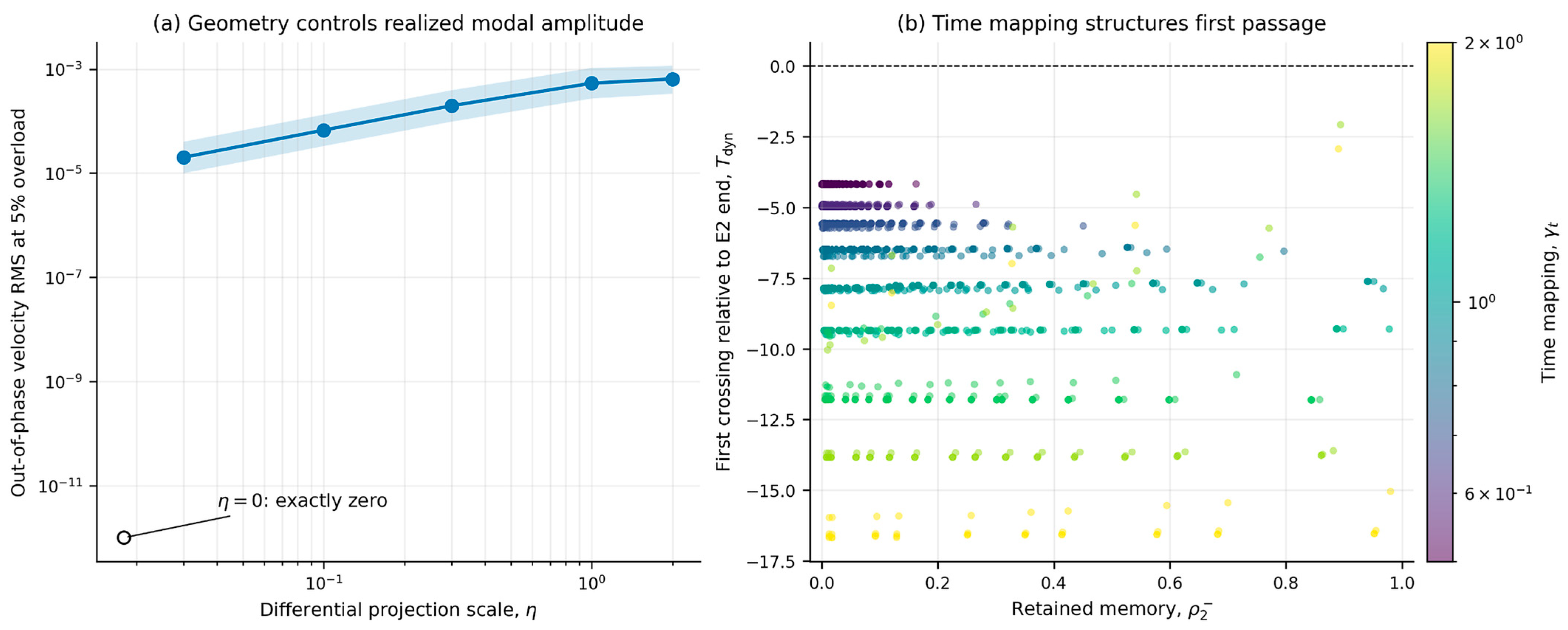
The first unstable mode is antisymmetric and therefore requires a differential forcing component for its direct excitation. In all 220 admissible exact-symmetry sequence simulations, $\eta =0$ produced zero antisymmetric amplitude to machine precision. Common forcing could still generate memory and move the frozen system beyond the antisymmetric stability boundary, but it could not realise finite antisymmetric motion in the absence of differential excitation.

For $\eta >0$, the post-event antisymmetric root-mean-square amplitude at 5% overload ranged from

$$1.371\times {10}^{-6}-7.814\times {10}^{-3}$$

(60)

Within

$$\eta \in \left\{\mathrm{0.03,0.1,0.3}\right\}$$

(61)

the median log–log slope was 0.9913, indicating an approximately linear dependence on differential forcing amplitude. No imperfection-insensitive finite-amplitude plateau was observed.

These results require a distinction between crossing the latent antisymmetric stability boundary and realising finite antisymmetric motion. They also show that the dimensionless modal amplitude cannot be interpreted as a universal prediction of physical displacement.

First-passage times formed distinct bands controlled by ${\gamma }_{\mathrm{t}}$, because this mapping parameter modifies both the duration of the accelerogram in model time and its position relative to $T_{\mathrm{d}\mathrm{y}\mathrm{n}}$. The simulations therefore do not identify a transferable physical delay, in seconds, between the onset of shaking and slope failure.

These geometry and time-mapping effects are summarised in Figure 8: panel (a) shows the dependence of realised antisymmetric amplitude on differential forcing, and panel (b) shows the corresponding first-passage-time structure.

3.5. Mainshock Memory Shifts Stochastic Activation Curves

All 33 primary stochastic parameter cells satisfied

$${\lambda }_{50}^{({\mathrm{E}}_1\to {\mathrm{E}}_2)}<{\lambda }_{50}^{\left({\mathrm{E}}_2\mathrm{o}\mathrm{n}\mathrm{l}\mathrm{y}\right)}$$

(62)

on the basis of the point estimates. Paired 95% bootstrap confidence intervals (CIs) excluded zero in 32 cells. The only unresolved case was the intentionally weak-memory white-noise sensitivity; its point estimate nevertheless retained the same direction of change. No realisation activated in either the primary or confirmation ensembles.

The 4096-realisation confirmation ensembles at

$$D={\displaystyle \frac{D_{\mathrm{m}\mathrm{a}\mathrm{x}}}{4}}=7.906\times {10}^{-7}$$

(63)

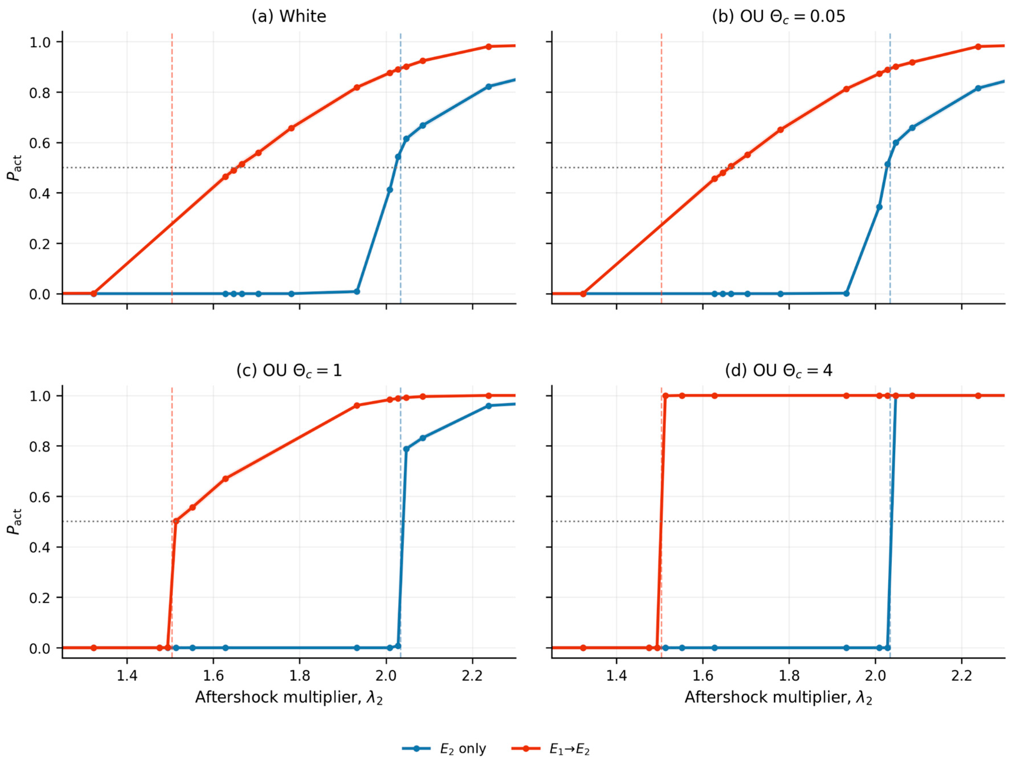
produced threshold reductions ranging from 18.00% to 26.21% (

Table 4. Confirmation stochastic thresholds and paired uncertainty.

Noise Condition	λ50, E2 Only (95% CI)	λ50, Sequence (95% CI)	Reduction (95% CI)
White	2.022 [2.018, 2.025]	1.655 [1.624, 1.682]	18.16% [16.80, 19.66]
OU, Θc = 0.05	2.027 [2.024, 2.032]	1.662 [1.631, 1.682]	18.00% [17.04, 19.52]
OU, Θc = 1	2.040 [2.040, 2.040]	1.513 [1.512, 1.534]	25.84% [24.80, 25.88]
OU, Θc = 4	2.038 [2.038, 2.038]	1.504 [1.504, 1.504]	26.21% [26.21, 26.21]

). White noise and short-correlated Ornstein–Uhlenbeck forcing with ${\Theta }_{\mathrm{c}}=0.05$ produced closely comparable thresholds. At ${\Theta }_{\mathrm{c}}=1$ and 4, the stochastic sequence thresholds approached the deterministic reference, and the corresponding reductions were close to 26%.

Figure 9 displays the corresponding confirmation activation curves, and Table 4 reports the numerical median thresholds and paired 95% bootstrap intervals for the four confirmation noise conditions.

3.6. Healing Progressively Removes the Stochastic Interaction

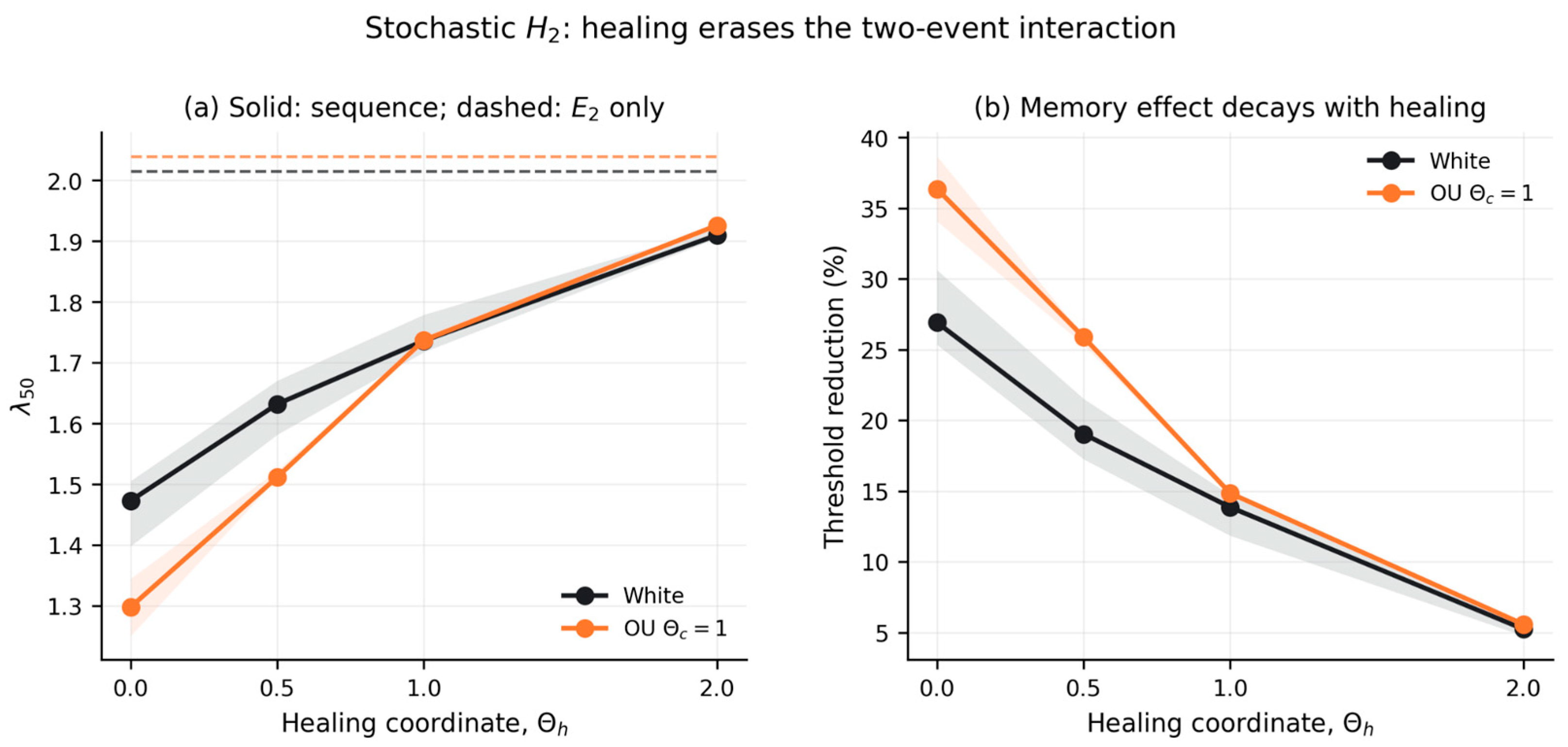
At $D={\displaystyle \frac{D_{\mathrm{m}\mathrm{a}\mathrm{x}}}{4}}$, the sequence median activation threshold ${\lambda }_{50}$ increased monotonically over

$${\Theta }_{\mathrm{h}}\in \{\mathrm{0,0.5,1},2\}$$

(64)

for both white noise and Ornstein–Uhlenbeck forcing with ${\Theta }_{\mathrm{c}}=1$.

Under white-noise forcing, the threshold reduction decreased from 26.91% to 5.24%. Under Ornstein–Uhlenbeck forcing, it decreased from 36.35% to 5.57%. In both cases, the sequence thresholds approached their respective $E_2$-only limits.

Figure 10 uses D = Dmax/4 as a representative intermediate stochastic-intensity case. This value was not selected from the earthquake outcomes: the admissible noise range was fixed beforehand by the no-earthquake pilot, and D = Dmax/4 lies between the weakest and upper admissible primary intensities. It is therefore illustrative rather than a uniquely typical field condition.

$${\rho }_1{e}^{-\mathsf{\Theta }\mathrm{ₕ}}$$

(65)

tended toward zero. The stochastic recovery trend therefore reproduces the deterministic healing limit. It is inconsistent with either a permanent event label or a simple unrelaxed addition of the two earthquake inputs.

3.7. The Influence of Noise Colour Depends on Correlation Time

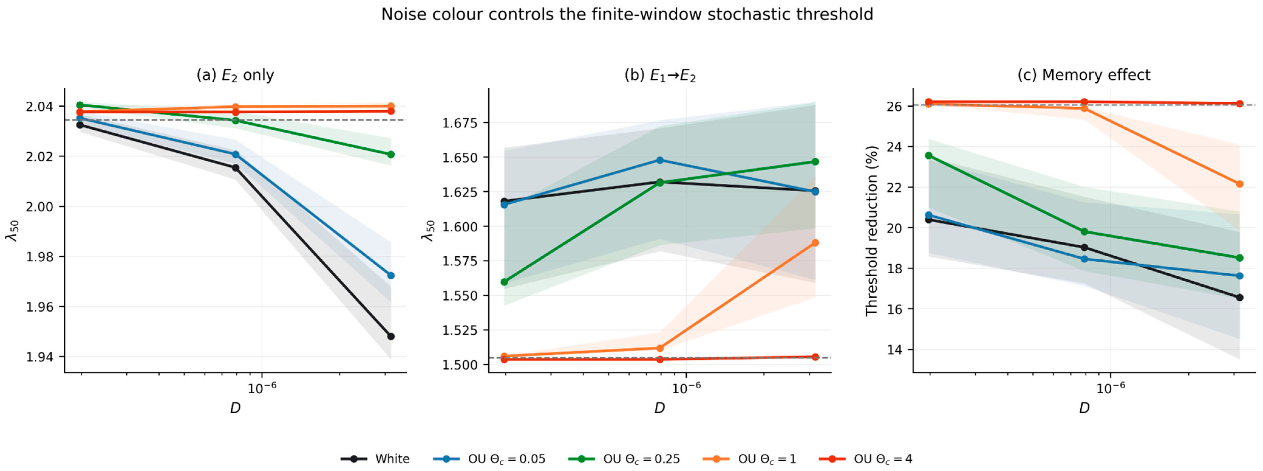
Direct paired comparisons between white-noise and Ornstein–Uhlenbeck forcing at $D={\displaystyle \frac{D_{\mathrm{m}\mathrm{a}\mathrm{x}}}{4}}$ showed no resolved difference in threshold reduction at ${\Theta }_{\mathrm{c}}=0.05$ or 0.25. The Ornstein–Uhlenbeck-minus-white differences were −0.23 percentage points, with a 95% confidence interval of −1.39 to 0.89, and +0.34 percentage points, with a 95% confidence interval of −1.45 to 1.50, respectively.

At ${\Theta }_{\mathrm{c}}=1$, the Ornstein–Uhlenbeck threshold reduction exceeded the white-noise reduction by 6.44 percentage points, with a 95% confidence interval of 2.80–7.98. At ${\Theta }_{\mathrm{c}}=4$, the difference was 6.77 percentage points, with a 95% confidence interval of 3.03–8.46.

Under the adopted fixed integrated-intensity normalisation, increasing ${\tau }_{\mathrm{c}}$ reduces the forcing variance accumulated over the finite earthquake window and produces a progressively smoother input. Long-correlated Ornstein–Uhlenbeck forcing therefore approached the deterministic thresholds in the present experiments.

This result does not imply a universal ordering between coloured and white noise. The observed contrast depends on the adopted normalisation, earthquake duration, dynamical response filter, and observation window.

Figure 11 provides the corresponding across-intensity comparison and confirms that the qualitative direction of the paired memory effect is not restricted to the D = Dmax/4 example used in Figure 10.

3.8. Control Experiments Isolate the Proposed Mechanism

Resetting the memory state after $E_1$ restored $\chi =0$ and produced an $E_2$ response that was bitwise identical to the corresponding $E_2$-only simulation. The maximum difference across all paired metrics was exactly zero.

In the no-delay control, the numerical value ${\chi }_{\mathrm{c}}$ could still be exceeded, but it no longer represented the stability boundary of the modified system. The registered probability of delayed activation was zero. Exact common forcing combined with fully correlated block noise likewise produced exactly zero antisymmetric displacement.

No-earthquake activation was absent in all primary controls, and no numerical divergences occurred.

Changing the matched no-event response percentile from 0.99 to either 0.95 or 0.999 did not reverse the direction of the memory effect, although the reference threshold reduction varied from 14.35% to 26.21%.

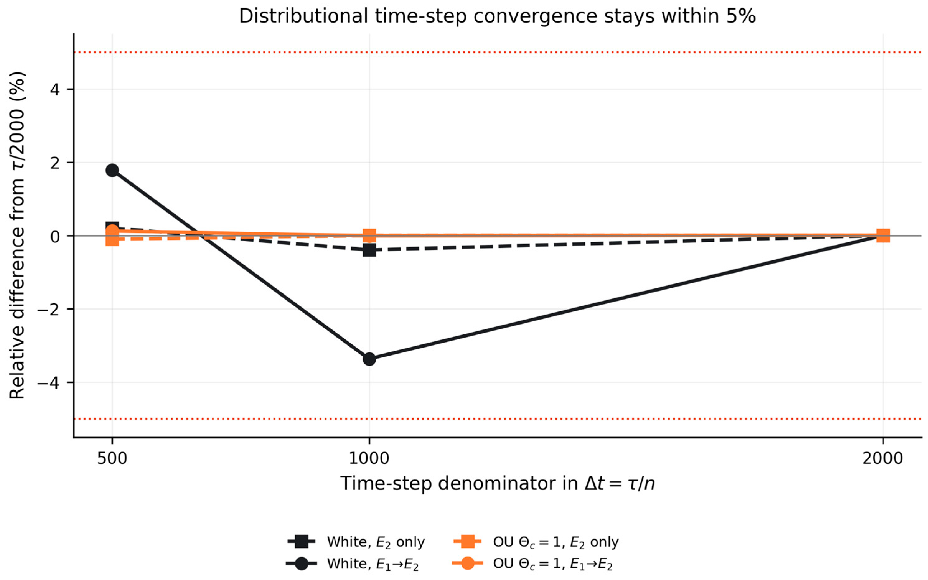
The stochastic calculations at

$$\Delta t={\displaystyle \frac{\tau }{500}},{\displaystyle \frac{\tau }{1000}},{\displaystyle \frac{\tau }{2000}}$$

(66)

remained within 3.37% of the finest-grid estimate of ${\lambda }_{50}$, satisfying the prespecified 5% convergence tolerance. The deterministic compiled and Python 3.13.5 implementations agreed to a maximum absolute metric difference of

$$2.22\times {10}^{-16}$$

(67)

Together, these controls show that the observed threshold reduction depends on the interaction between response-generated memory and delayed mechanical instability. It cannot be reproduced by earthquake concatenation alone, common-mode forcing, numerical discretisation, solver implementation, or a permanent event-specific modification.

4. Discussion

4.1. Causal Identification of Inherited Susceptibility

The principal finding of this study is that, within the proposed framework, a non-activating earthquake can transiently reduce the activation threshold of a subsequent earthquake through an inherited mechanical state generated exclusively by the intervening response. This distinction is fundamental. The first earthquake is absent when the second begins, it never satisfies the activation criterion, and it cannot influence the second event through prescribed cumulative damage or event-based parameter updates. Its only surviving effect is the response-generated memory state. Consequently, the observed threshold reduction is attributable to retained susceptibility rather than to the addition of seismic input.

Three independent observations support this causal interpretation. First, the threshold reduction is almost perfectly monotonic in the retained memory state, ${\rho }_2^{-}$. Second, progressive healing continuously restores the sequence threshold to the aftershock-only limit. Third, resetting the memory state reproduces the aftershock-only response exactly. Together, these controls distinguish inherited susceptibility from simple earthquake addition. If the observed threshold reduction resulted only from concatenating two acceleration records or from numerical inconsistencies between the paired experiments, neither continuous recovery nor exact restoration under memory reset would be expected.

This interpretation complements rather than replaces previous sequence studies. Existing investigations demonstrate that successive earthquakes can increase displacement, modify reliability, and interact through waveform characteristics such as duration, polarity, or spatial variability [8,9,10,11]. The present work addresses a different scientific question. Instead of asking how much additional displacement results from two earthquakes, it asks whether the mechanical consequences of a non-activating first event can themselves be isolated as the causal mechanism responsible for lowering the activation threshold of the second event. The distinction is therefore between cumulative forcing and inherited susceptibility.

The scalar memory coordinate $\chi$ is intentionally introduced as a coarse-grained dynamical state rather than as a material property. It summarises the mechanical consequences of prior loading—including crack evolution, pore-pressure redistribution, contact ageing, and shear-zone fabric—without attempting to resolve each mechanism individually. Its purpose is not to reproduce a specific constitutive process but to represent their shared dynamical characteristic: susceptibility increases during shaking and gradually recovers afterwards. The response-generated evolution law and continuous healing enforce this behaviour while remaining consistent with laboratory and field evidence for fatigue, weakening, metastability, and recovery [15,20,21,22]. Future site-specific formulations may replace $\chi$ with measurable state variables appropriate for particular materials and failure mechanisms without altering the causal framework developed here.

Material degradation and inelasticity therefore enter the present framework only in coarse-grained form. Repeated loading can increase χ and temporarily reduce effective resistance, but the model does not prescribe how crack density, accumulated plastic strain, stiffness, cohesion, friction angle, or pore pressure evolve individually. The added ±2.5% one-at-a-time sensitivity of a, b, and c provides a local numerical test of constitutive dependence: after recomputing the stability boundary for each perturbation, all six admissible cases retained λ₂, seq < λ₂, only, with threshold reductions of 20.673–36.842%. This supports robustness of the directional mechanism to modest constitutive changes without implying a calibrated law of material degradation or strain softening.

This distinction also defines the engineering interpretation of χ. Because χ acts only through the fractional reduction of incremental resistance, the observable quantity to be calibrated is not χ in isolation but the relationship between measurable postseismic state changes and effective resistance. For a pore-pressure-dominated soil slope, χ could be linked primarily to effective-stress loss; for a fractured rock slope, it could be linked more strongly to damage, contact degradation, or stiffness reduction. Different observation operators may therefore represent the same reduced-order state without implying that the underlying material physics are identical.

4.2. Delay Creates the Instability; Memory Controls Its Accessibility

Memory and delay perform fundamentally different dynamical functions. The memory state modifies incremental resistance and thereby controls the accessibility of instability, whereas displacement delay provides the mechanism through which the instability itself arises. This separation is essential because it prevents the proposed framework from collapsing into a generic accumulated-damage model.

The same caution applies to τ. Its role in the present paper is dynamical, not diagnostic: τ is the delay coordinate that enters the characteristic equation and permits the out-of-phase Hopf crossing. Whether field-scale delays generated by stress transfer, shear-zone processes, wave propagation, or hydrological redistribution place a particular slope in the Hopf-capable range remains an empirical calibration question. The parameter sweep therefore demonstrates a mechanism and its local robustness, not a universal engineering range of delay times.

Exceeding the numerical value of ${\chi }_c$ in the $\tau = 0$ control does not constitute evidence of the same instability, since removing delay changes the characteristic equation and therefore the underlying stability problem. The no-delay control demonstrates that memory alone is insufficient to reproduce the observed behaviour. Conversely, delay alone cannot explain the systematic threshold reduction observed after a subcritical first earthquake. Only their interaction produces the identified mechanism.

The first unstable mode is antisymmetric and therefore requires a differential forcing component for its excitation. The northeast and southeast cliff-face projections provide one physically explicit source of such differential loading. The common-mode control further demonstrates that the loss of frozen-system stability is not equivalent to finite antisymmetric motion. Likewise, the nearly linear small-$\eta$ scaling explains why the reduced-order model should not be interpreted as predicting universal displacement amplitudes. A quantitative prediction of physical displacement would require independently constrained wave propagation, topographic amplification, spatial heterogeneity, and local transfer functions.

4.3. The Conditional Influence of Noise Colour

The stochastic comparison was intentionally formulated so that Ornstein–Uhlenbeck forcing converges to the declared white-noise model as ${\tau }_c \to 0$. The close agreement observed for ${\Theta }_c = 0.05$ and ${\Theta }_c = 0.25$ therefore provides an important limiting consistency check. Differences emerge only when the correlation time becomes comparable to or exceeds the characteristic timescale of the delayed dynamics.

The direction of these differences follows directly from the adopted normalisation. At fixed long-time diffusion intensity, a strongly correlated Ornstein–Uhlenbeck process exhibits smaller finite-window variance than white noise over the duration of the recorded earthquake. Consequently, the corresponding activation thresholds remain closer to the deterministic limit. The influence of noise colour is therefore conditional rather than universal: it becomes significant only when the intrinsic timescale of the stochastic forcing competes with that of the delayed mechanical response. Future work comparing fixed stationary variance, continuous forcing throughout the inter-event period, and alternative observation windows will establish which aspects of this behaviour remain invariant across forcing conventions.

From a field perspective, Θc should therefore be read as a ratio of environmental persistence to the intrinsic mechanical period rather than as a direct proxy for a particular loading source. Short-correlated microseismic or vibrational forcing may occupy Θc ≪ 1, whereas slowly varying thermal, anthropogenic, or hydrological influences may generate much longer correlations. Hydrological effects, however, can also alter effective stress and healing kinetics and should not be reduced to additive OU forcing in a site-specific model.

4.4. Engineering Implications and Corroboration from the Redcliffs Sequence

The broader implication of the present results is that earthquake-sequence hazard may depend not only on the incoming ground motion but also on the evolving internal state of the slope. Models treating each earthquake as an independent loading event may therefore overlook an important component of transient susceptibility, even when the second earthquake is represented accurately. Sequence-aware hazard assessment would require estimating, updating, and propagating the evolving recovery state together with its uncertainty throughout the interval separating successive earthquakes.

This interpretation is consistent with post-earthquake inventories demonstrating that landslide activity evolves over time [37,38,39] and with observations showing that hydrological, thermal, and seismic processes jointly influence rock-slope susceptibility [40]. Within this broader context, the present reduced-order model should be viewed as a transparent mechanistic framework for identifying and testing the consequences of inherited susceptibility rather than as a site-specific predictive model.

The Redcliffs sequence provides a particularly appropriate demonstration because the February and June 2011 earthquakes constitute a documented earthquake pair with corrected accelerograms recorded at a common station, while the two principal cliff faces define distinct geometric projections of the same seismic input. Without independent normalisation of the individual events, the model reproduces the predicted direction of threshold change under these recorded waveforms. The agreement does not constitute site calibration, but it demonstrates compatibility between the proposed causal mechanism and realistic geometry-dependent earthquake forcing. Site-specific validation will require the joint estimation of transfer amplitudes, ${\gamma }_t$, ${\alpha }_d$, healing parameters, and wave-propagation effects before quantitative predictions of displacement, probability of failure, or failed volume are attempted.

One should note that the primary numerical experiment remains centred on the physically documented February–June 2011 Redcliffs pair. The auxiliary Darfield–February calculation tests whether the directional result persists for a different first-event waveform and a longer inter-event interval while retaining the same HVSC station, Redcliffs geometry, and reduced-order model. The auxiliary pair produced a substantially smaller threshold reduction, 2.134% compared with 26.047% in the primary reference case, but preserved the same ordering λ₂, seq < λ₂, only. This supports the within-Canterbury cross-pair robustness of the causal direction but does not establish universality across recording sites, slope geometries, or geomaterials. Independent external sequence testing remains necessary before the magnitude of the threshold reduction can be considered transferable.

4.5. Future Research Directions

The present study identifies several connected directions for developing sequence-aware landslide prediction.

First, physical calibration should establish quantitative relationships between the dimensionless memory formulation and measurable slope response. The joint inversion of local ground motion, deformation monitoring, modal response, and recovery observations could constrain transfer functions, dynamical timescales, and the mapping between model activation and observable behaviour.

Second, the present two-block formulation should be extended to higher-dimensional systems, including block chains, interaction networks, and continuum descriptions. Such models would permit heterogeneous memory evolution, travelling localisation, topographic amplification, and multiple interacting instability modes while testing whether the identified causal mechanism remains operative at larger spatial scales.

Third, the coarse-grained memory coordinate should be replaced by constitutive formulations derived from laboratory and field observations. Candidate developments include non-exponential recovery, multiple interacting state variables, contact ageing, threshold effects, and coupled friction–hydrology formulations. Ring-shear experiments, repeated dynamic loading tests, ambient-vibration monitoring, and post-earthquake deformation records offer promising routes for identifying these constitutive relationships.

The added two-timescale sensitivity further defines the applicability boundary of the single-exponential healing law. The comparison does not identify either recovery law as universally more conservative: a dominant fast component can reduce retained susceptibility more rapidly at intermediate intervals, whereas a weaker slow component can preserve more memory at long intervals. The causal ordering of the paired thresholds nevertheless persisted throughout the tested bi-exponential cases. Site-specific prediction would still require the recovery timescales and weights to be independently constrained from laboratory or postseismic monitoring observations.

Fourth, the forcing formulation should be generalised to allow continuous environmental excitation throughout the recovery interval. Background seismicity, rainfall, hydrological transients, and environmental vibrations could then modify the inherited state between major earthquakes, enabling the direct investigation of coupled seismic and hydro-mechanical preconditioning.

Hydrological coupling should be introduced as a state-dependent process rather than merely as additive noise. Rainfall infiltration can change pore pressure, effective stress, and the apparent healing rate, while drainage and suction recovery can produce the opposite effect. The local friction-law sensitivity added in this revision partially addresses dependence on the inherited coefficients a, b, and c: independent ±2.5% perturbations changed both the stability boundary and the magnitude of threshold reduction, but all six admissible cases retained a lower sequence threshold. This supports local constitutive robustness without implying material universality. The perturbation range is not assigned to clays, soft rocks, hard rocks, or fractured rock masses; such applications require independently constrained material-specific friction laws, parameter ranges, and coupled hydro-mechanical state variables.

Finally, the auxiliary Darfield–February calculation provides one additional within-Canterbury event pairing but is not an independent validation ensemble. Broader validation should still incorporate external earthquake sequences, slope materials, geometries, and recording configurations spanning different mainshock–aftershock magnitude contrasts, inter-event times, and frequency contents, with a recalibration of the physical time, resistance, and observation mappings for each site. Hierarchical calibration with uncertainty propagation and prospective post-mainshock monitoring would provide a stronger test of whether state-aware forecasts consistently outperform event-independent threshold models.

Taken together, these results demonstrate that transient susceptibility can emerge naturally as a consequence of prior mechanical response without prescribing cumulative damage. Within the limits of a reduced-order dynamical model, the proposed framework therefore identifies a causal mechanism by which a non-activating earthquake can temporarily reduce the activation threshold of a subsequent event. This distinction between cumulative forcing and inherited susceptibility provides a physically interpretable basis for incorporating earthquake-sequence effects into future state-aware models of landslide hazard.

5. Conclusions

This study identifies a path-dependent mechanism through which a non-activating earthquake can transiently increase the susceptibility of a slope to a subsequent event. In the proposed delayed two-block framework, the first earthquake generates a bounded internal state exclusively through the computed dissipative response, and heals continuously between events. The critical memory level is derived independently from the characteristic roots of the delayed mechanical subsystem. By holding the second-earthquake waveform and model coordinates fixed, the paired sequence and second-event-only experiments isolate the inherited-state effect rather than the simple addition of two acceleration records.

The deterministic calculations show that the mechanism is systematic within the admissible domain. Of 324 simulations, 251 remained non-activating and generated 1255 paired threshold comparisons across healing levels. Every comparison produced a lower sequence threshold, while the unresolved interval comparisons occurred only under strong healing and converged toward the second-event-only limit. Retained memory accounted for almost all rank variation in threshold reduction. At the reference parameter combination, the second-event activation threshold was reduced by approximately 26%, demonstrating that the operative sequence variable is the state present when the later earthquake begins.

The same directional result persisted under stochastic forcing. All 33 primary stochastic parameter cells yielded lower sequence thresholds, and 32 paired 95% bootstrap confidence intervals excluded zero. The 4096-realisation ensembles produced threshold reductions of approximately 18–26% under white-noise and Ornstein–Uhlenbeck forcing. Increasing healing progressively restored sequence thresholds toward their second-event-only limits. Resetting the memory state reproduced the second-event-only response, while removing displacement delay eliminated registered delayed activation. These controls support the interpretation that the threshold shift arises from the interaction between retained susceptibility and delayed mechanical instability.

Three targeted robustness analyses tested key modelling assumptions. A weighted bi-exponential healing law preserved the lower sequence threshold while showing that the quantitative effect depends on fast and slow recovery. Independent ±2.5% perturbations of the friction-law coefficients preserved the causal direction in all six admissible cases. An auxiliary Darfield–February Canterbury pairing also retained the same threshold ordering but produced a much smaller reduction, consistent with the smaller inherited state generated by the Darfield record. These tests support robustness of the directional mechanism without implying a universal effect magnitude.

The engineering implication is that the intensity and waveform of a later earthquake may be insufficient descriptors of sequence-dependent slope hazard when the slope has not fully recovered from previous shaking. The Redcliffs calculations demonstrate the mechanism under documented geometry-dependent forcing without event-specific normalisation. However, the model remains dimensionless and mechanism-identifying rather than site-calibrated. The reported threshold reductions should therefore not be transferred directly to other slopes, materials, or earthquake sequences.

Quantitative application will require independent constraints on the mapping between the memory coordinate and measurable postseismic state variables, together with the calibration of time mapping, delay, healing kinetics, hydrological effects, geomaterial response, local ground-motion transfer, and physical failure observables. Within these limits, the central conclusion is that earthquake-sequence landslide initiation is more appropriately viewed as a state-dependent trajectory problem than as a succession of independent event-by-event thresholds.