An Inspection-Driven Decision-Support Framework for Deterioration Prediction and Maintenance Optimization of Highway Bridges Without Historical Inspection Records

Abstract

Maintenance planning for highway bridges without historical inspection records remains challenging because conventional deterioration models typically require long-term data for calibration. This study proposes an inspection-driven decision-support framework that integrates bridge-specific engineering calibration, Markov deterioration modelling, an independent condition-rating-based Remaining Service Life (RSL) assessment, and Markov Decision Process (MDP) optimization. The framework was demonstrated on a 26-year-old six-span composite highway bridge in Türkiye. A comprehensive inspection yielded a weighted Bridge Condition Index of 2.98, which was used to calibrate the bridge-specific Markov deterioration model. The model predicted attainment of the State-4 intervention threshold after approximately 15.71 years under a do-nothing scenario, while the independent condition-rating assessment estimated an RSL of approximately 17 years for the governing pier columns. The optimized finite-horizon MDP policy reduced the expected discounted life-cycle cost by 89.75% relative to the do-nothing strategy, while sensitivity analyses confirmed the stability of the principal maintenance policy under the examined modelling and economic perturbations. The proposed framework therefore provides a practical, transparent, and progressively updateable methodology for deterioration prediction and maintenance planning for bridges with limited historical inspection information.

1. Introduction

Highway bridges are strategic components of transportation networks, and their uninterrupted serviceability is essential for economic and social continuity. As bridge stocks continue to age worldwide, infrastructure owners face the dual challenge of evaluating current structural condition and predicting future deterioration so that limited maintenance resources can be allocated effectively. Bridge Management Systems (BMSs) have been developed to support this process by integrating systematic inspection, condition assessment, deterioration modelling, and maintenance planning within a unified decision-support environment [1,2]. Among these components, periodic visual inspection remains the primary source of condition information because it is rapid, economical, non-destructive, and forms the basis for condition-state records used in bridge management practice [3,4].

Among the deterioration modelling techniques adopted in BMS applications, discrete-state Markov chains remain the most widely used stochastic approach because of their ability to represent the uncertainty associated with structural deterioration. Early studies demonstrated the applicability of Markov models for bridge performance prediction and transition probability estimation using long-term inspection records [2,5,6]. Subsequent research further established Markov models for bridge deck performance prediction [7], bridge element deterioration assessment [8], and risk-based bridge management [9]. More recent developments include non-homogeneous and continuous-time Markov formulations [10,11], semi-Markov deterioration models [12,13], bridge-type-specific deterioration models [14], optimization-assisted transition probability calibration [15], hybrid real–synthetic inspection datasets [16], and multi-model deterioration frameworks that reduce prediction uncertainty [17]. In parallel, digital-twin platforms and inspection-data-driven machine learning models have recently begun to couple inspection information directly with predictive deterioration modelling and maintenance decision-making [18,19,20,21]. Despite these methodological advances, virtually all existing approaches rely on multi-year inspection databases to establish statistically reliable deterioration models.

This dependence on historical inspection data represents one of the principal limitations of Markov-based deterioration modelling. Reliable transition probability matrices generally require repeated condition observations collected over many inspection cycles [5,22], yet such information is unavailable for a considerable number of existing highway bridges. In Türkiye, the General Directorate of Highways (KGM) has established standardized visual inspection procedures and element-based bridge evaluation methodologies, and significant progress has been achieved toward a national BMS [23,24,25,26]. However, numerous bridges owned by municipalities, universities, and other public institutions have never been incorporated into a systematic inspection program. For these structures, condition-rating-based RSL methodologies developed by Yanmaz et al. [27], Caner et al. [28], and Berk [29] provide practical engineering approaches for estimating service life from a single comprehensive condition assessment. Nevertheless, these methods do not explicitly model stochastic deterioration or maintenance optimization.

On the maintenance decision side, MDPs provide a rigorous mathematical framework for determining optimal maintenance actions under uncertain deterioration [30,31,32]. Recent studies have expanded MDP applications through seismic deterioration modelling [33,34], Bayesian inspection-maintenance integration [35], and reinforcement learning techniques for large-scale infrastructure management [36,37,38,39,40,41,42]. Although these studies demonstrate the maturity of optimization-based maintenance planning, they likewise assume the availability of calibrated deterioration models and maintenance-effect relationships derived from extensive historical datasets.

Despite the substantial progress achieved in deterioration modelling and maintenance optimization, practical decision-making remains difficult for existing highway bridges without historical inspection records. Most previous studies have focused on deterioration prediction, RSL estimation, or maintenance optimization as independent research topics, whereas relatively limited attention has been given to integrating these complementary approaches into a unified decision-support framework for bridges lacking historical inspection data. In particular, guidance remains limited on how a detailed bridge inspection can be systematically transformed into deterioration prediction and subsequently into optimized maintenance decisions when long-term condition records are unavailable.

The present study addresses this challenge by proposing an inspection-driven integrated framework for bridge deterioration prediction and maintenance optimization. The framework combines a harmonized five-state bridge condition assessment procedure, a weighted Bridge CI, bridge-specific engineering calibration of a Markov deterioration model, an independent condition-rating-based RSL assessment used as an engineering benchmark, and MDP-based maintenance optimization within a unified computational workflow. Rather than introducing new deterioration or optimization algorithms, the proposed methodology integrates established engineering techniques into a practical and transferable decision-support framework specifically designed for highway bridges without historical inspection records. The novelty of the study is therefore an integration novelty rather than an algorithmic one: the contribution lies in (i) demonstrating how a single comprehensive inspection can be systematically transformed into a calibrated stochastic deterioration model through a transparent, constraint-based engineering calibration procedure; (ii) cross-checking the resulting predictions against an independent condition-rating-based RSL assessment; and (iii) closing the loop from inspection to optimized maintenance decisions within a single reproducible computational workflow that can be progressively updated as inspection data accumulate.

The objectives of this study are to: (1) perform a systematic element-level condition assessment of an existing highway bridge without historical inspection records; (2) establish a weighted Bridge CI using a harmonized five-state condition rating system; (3) predict future deterioration through a bridge-specific Markov deterioration model developed using an inspection-driven engineering calibration procedure; (4) independently assess the RSL using a condition-rating-based engineering methodology; (5) determine the optimal maintenance policy using a MDP; and (6) demonstrate an integrated and transferable decision-support framework that can be progressively refined as additional inspection and maintenance information become available for future BMS applications.

2. Description of the Case-Study Bridge

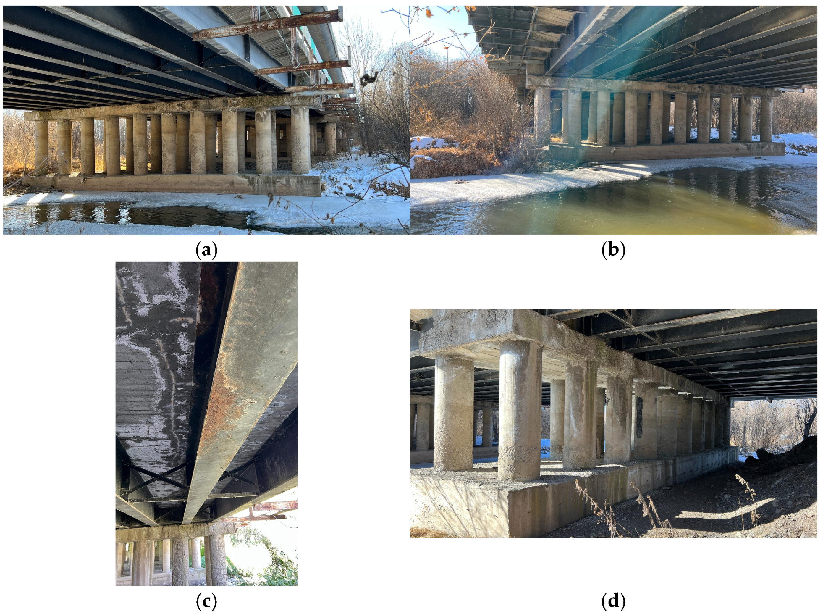
The case-study bridge is a composite highway bridge crossing the Kars River within the Kafkas University campus in Kars, northeastern Türkiye, connecting the eastern and western precincts of the campus. The bridge has been in continuous service since 2000 and carries two traffic lanes (one in each direction) without a central median, while the four-lane approach roads narrow over the bridge. General views of the bridge and its principal structural components are presented in Figure 1.

The bridge consists of a reinforced concrete deck supported by steel I-girders, reinforced concrete intermediate piers, elastomeric bearings, and steel cross-bracing systems. During the field investigation, it was confirmed that although the bridge was originally designed with seven spans, it was constructed with six spans because one intermediate pier was omitted during construction for undocumented reasons. This discrepancy between the archived design drawings and the as-built structure highlights the importance of field verification in bridge condition assessment.

The 15 m wide reinforced-concrete deck acts compositely with twelve steel I-section main girders, each approximately 700 mm deep with 300 mm wide and 20 mm thick flanges, and is laterally stabilized by steel cross-bracing provided at 6 m intervals. Each intermediate pier comprises twenty reinforced-concrete columns arranged in two rows of ten, with an approximately 2.15 m free column height beneath 450 mm deep transverse cap beams; load transfer to the substructure is provided through 35 mm thick elastomeric bearings measuring approximately 400 mm × 460 mm in plan. The substructure includes foundations and piles, while reinforced-concrete base platforms measuring approximately 3.10 m × 15 m × 1.60 m were subsequently constructed around the pier columns; the geometric information used in the study was established from archived drawings together with field measurements.

A further as-built modification was identified during the field inspection. Following ground-related stability problems reported during the early years of service, reinforced concrete base platforms (buttress blocks) were constructed around the intermediate pier columns to improve structural stability. Since neither the omitted pier nor this retrofit is documented in the original archive drawings, all geometric and structural information used in this study was established by combining archived design documents with detailed field observations.

Table 1. Element inventory of the case-study bridge.

Superstructure Elements	Substructure Elements	Service Components
Deck slab	Abutments	Wearing surface (asphalt)
Steel main girders	Intermediate piers (columns)	Expansion joints
Elastomeric bearings	Pier cap beams	Drainage system
Steel cross-bracings	Approach fill and approach slab	Curbs and sidewalks
	Slope/scour protection works	Railings and barriers
	Foundations and piles

summarizes the bridge elements considered in the condition assessment, grouped into superstructure, substructure, and service components according to standard BMS practice [4,43].

3. Methodology

3.1. Bridge Inspection and Condition Assessment

Two comprehensive visual inspection campaigns were conducted during the winter (February 2025) and summer (August 2025) to account for seasonal variations in environmental conditions and to improve the reliability of the visual condition assessment. All bridge elements, including the superstructure, substructure, and service components, were systematically inspected. Visible deterioration mechanisms, including cracking, concrete spalling and delamination, reinforcement exposure and corrosion, water leakage, efflorescence, deformation, and scour-related distress, were documented using photographs and video records. No significant differences in the assigned condition states were observed between the two inspection campaigns; therefore, the findings were consolidated into a single inspection dataset, which forms the basis of the inspection-driven deterioration assessment framework.

The condition of each bridge element was initially evaluated using the four-grade visual inspection system recommended by the Turkish General Directorate of Highways (KGM), where Grades A–D represent increasing levels of deterioration and the corresponding maintenance requirements [23]. To provide a condition-state representation compatible with the five-state Markov deterioration model adopted in this study, the KGM classification was harmonized into a five-state condition rating system. This harmonized classification preserves the engineering interpretation of the original KGM methodology while providing an appropriate condition-state definition for deterioration prediction and subsequent maintenance optimization. The adoption of a five-state representation is also consistent with previous bridge deterioration studies employing discrete-state Markov models [2,7]. The resulting harmonized condition rating system is presented in

Table 2. Harmonized five-state bridge condition rating system.

KGM Class	Condition	Description	Condition State
A	Very good	No damage, or damage at a negligible level; no defect affecting structural or functional performance	1
B	Good	Light surface deterioration; element functionality preserved; monitoring and routine maintenance only	2
C	Fair	Distinct deterioration; element performance partly affected; maintenance or repair should be planned in the near term	3
D	Poor	Advanced damage; element performance substantially reduced; priority maintenance and repair required	4
D/E *	Very poor	Element has largely lost its function or exhibits critical damage; urgent intervention or replacement required	5

* The fifth condition state was introduced to establish compatibility between the KGM visual inspection methodology and the five-state Markov deterioration framework employed in this study while preserving the engineering interpretation of the original KGM classification.

.

3.2. Bridge Condition Assessment Method

Following the element-level condition assessment described in the previous section, the current condition of the bridge was quantified using a hierarchical aggregation procedure consistent with component-oriented BMS principles. Rather than assigning equal importance to all bridge elements, the proposed methodology considers both the observed condition state and the structural significance of each component within the overall load-transfer system. Consequently, deterioration affecting primary structural members contributes more to the overall bridge condition than deterioration of secondary or service-related components, consistent with established bridge management practice [2,4,5,7,43].

The bridge condition assessment was performed using a two-level hierarchical weighting procedure. First, bridge elements within each structural subsystem were assigned relative importance coefficients according to their structural function, load-transfer role, deterioration consequences, and maintenance priority, from which subsystem condition indices were calculated. Second, the subsystem condition indices were combined using bridge-level weighting coefficients representing the relative importance of the superstructure, substructure, and service systems. This hierarchical approach preserves the influence of local deterioration while providing a quantitative measure of the overall bridge condition. The adopted weighting factors and the resulting condition indices are presented in Section 4.

The weighting coefficients were assigned directly through engineering judgement informed by established BMS principles, the structural characteristics of the investigated bridge, and the observed deterioration pattern, rather than being generated through a formal numerical scoring or multi-criteria optimization procedure. Four explicit qualitative criteria were considered for each element: (i) its role in the vertical and lateral load-transfer path; (ii) the degree of structural redundancy associated with its potential failure; (iii) the consequences of its deterioration for structural safety and serviceability; and (iv) its influence on the deterioration of adjacent components (e.g., drainage deficiencies accelerating substructure corrosion). Accordingly, no separate numerical criterion-score matrix was used to derive the adopted coefficients; the numerical weighting inputs consist of the subsystem and within-subsystem coefficients documented in Appendix A (

Table A1. Two-level derivation of the element-level weighting coefficients.

Subsystem	Element	Within-Subsystem Weight	Subsystem Weight Wk	Bridge-Level Weight wi
Superstructure	Deck slab	0.30	0.35	0.1050
Superstructure	Steel main girders	0.35	0.35	0.1225
Superstructure	Steel cross-bracings	0.15	0.35	0.0525
Superstructure	Elastomeric bearings	0.20	0.35	0.0700
Substructure	Pier columns	0.30	0.45	0.1350
Substructure	Pier cap beams	0.20	0.45	0.0900
Substructure	Abutments	0.20	0.45	0.0900
Substructure	Approach fill/slab	0.075	0.45	0.0338
Substructure	Slope protection	0.075	0.45	0.0338
Substructure	Foundations/platform	0.15	0.45	0.0675
Service	Wearing surface	0.25	0.20	0.0500
Service	Expansion joints	0.25	0.20	0.0500
Service	Drainage system	0.25	0.20	0.0500
Service	Curbs/sidewalks	0.125	0.20	0.0250
Service	Railings/barriers	0.125	0.20	0.0250

). It is acknowledged that formal multi-criteria weighting techniques, such as the Analytic Hierarchy Process (AHP), Delphi-based expert surveys, entropy weighting, or Bayesian weight elicitation, provide more systematic alternatives for weight determination; these techniques, however, require panels of independent experts or statistical samples of comparable structures, neither of which was available for the investigated single-bridge application. To compensate for the subjectivity inherent in direct weight assignment, the sensitivity of the resulting condition index to the adopted weighting coefficients was quantitatively evaluated, as reported in Section 4.2, and the framework was deliberately formulated so that alternative weighting schemes can be substituted without modifying any other component of the methodology. The complete hierarchical derivation of the element-level weights from the within-subsystem coefficients and the subsystem weights is documented in Appendix A (Table A1).

The overall Bridge CI was computed as

$$CI={\displaystyle \sum _{k=1}^m}{W}_k{CI}_k$$

(1)

where ${CI}_k$ denotes the condition index of subsystem $k,W_k$ is the corresponding bridge-level weighting coefficient, and m is the number of principal bridge subsystems. The subsystem condition indices are obtained from the weighted aggregation of the inspection-derived element condition states.

For deterioration modelling, the inspection results were further transformed into an initial condition-state probability vector, Q(0), representing the proportion of the total bridge importance associated with each condition state. Unlike a simple frequency distribution, this formulation incorporates the structural importance of each bridge element and therefore preserves the engineering significance of the observed deterioration. The initial state vector is defined as

$$q_j\left(0\right)={\displaystyle \frac{{\displaystyle {\sum }_{i=1}^n}{w}_{i}I(s_i=j)}{{\displaystyle {\sum }_{i=1}^n}{w}_i}}, j=1,\dots ,5$$

(2)

where w_i denotes the bridge-level importance weight assigned to element i, s_i is the corresponding inspection-derived condition state, and I(⋅) is the indicator function. The inspection-derived condition indices and the corresponding condition-state distribution obtained using this procedure are presented in Section 4. The Bridge Condition Index provides the observed age-condition target for the calibration described in the following section, whereas the inspection-derived distribution is used only as the initial condition for forward deterioration prediction from the inspection date.

In this formulation, Q(0) should not be interpreted as the probability that the entire bridge occupies one mutually exclusive physical condition state. It represents the proportion of the total bridge-level importance weight associated with the assessed element categories assigned to each condition state. Each category was assigned a governing condition state from the consolidated visual-inspection evidence, and its bridge-level importance weight was then allocated to that state. The resulting vector is therefore an importance-weighted distribution over assessed element categories rather than a frequency distribution over individual physical units. Quantitative deterioration-extent fractions within each category were not recorded during the inspection campaigns and were not reconstructed retrospectively; accordingly, localized deterioration was represented conservatively through the governing category-level condition assignment.

3.3. Inspection-Driven Engineering Calibration of the Markov Deterioration Model

The future deterioration of the investigated bridge was modelled using a discrete-time, discrete-state homogeneous Markov chain. Markov deterioration models have been widely adopted in bridge management systems because they provide a probabilistic framework for representing progressive transitions between condition states under material ageing, environmental exposure, and traffic loading [2,5,6,7]. Under the Markov assumption, the future condition depends on the current condition state rather than on the complete preceding deterioration history [44,45].

Bridge deterioration was represented using the five condition states defined in Table 2, where State 1 denotes very good condition and State 5 represents a critical condition requiring major rehabilitation or replacement. Under the do-nothing assumption, deterioration was considered irreversible. During each annual transition interval, an element was therefore allowed either to remain in its current state or to deteriorate to the next adjacent state, while State 5 was treated as absorbing. These assumptions preserve row stochasticity, adjacent-state deterioration, and the absence of condition improvement without maintenance intervention [7,46].

For deterioration prediction, the inspection-derived vector $Q\left(0\right)$ represents the importance-weighted distribution of the assessed bridge elements among the five condition states. Its evolution after the inspection is expressed as

$$Q\left(t\right)=Q\left(0\right)\cdot P^t$$

(3)

where $P$ is the annual do-nothing transition probability matrix and t is the number of years after the current inspection. The corresponding expected condition indicator is calculated as

$$E\left(t\right)=Q\left(t\right)\cdot S^T, S=\left[1 2 3 4 5\right]$$

(4)

Because the investigated bridge has no longitudinal inspection database, the transition probabilities cannot be statistically estimated from observed state-to-state transitions using conventional maximum-likelihood, regression-based, or Bayesian procedures [2,22]. Moreover, a single inspection-derived condition observation does not provide sufficient information to identify four independent adjacent-state transition probabilities. To avoid an underdetermined calibration problem, the deterioration model was therefore deliberately reduced to a single annual adjacent-state deterioration parameter, p, giving

$$P\left(p\right)=\left[\begin{array}{ccccc}1-p& p& 0& 0& 0\\ 0& 1-p& p& 0& 0\\ 0& 0& 1-p& p& 0\\ 0& 0& 0& 1-p& p\\ 0& 0& 0& 0& 1\end{array}\right]$$

This parsimonious parameterization enables the available scalar condition information to identify a single deterioration parameter while retaining the principal physical constraints of the Markov process.

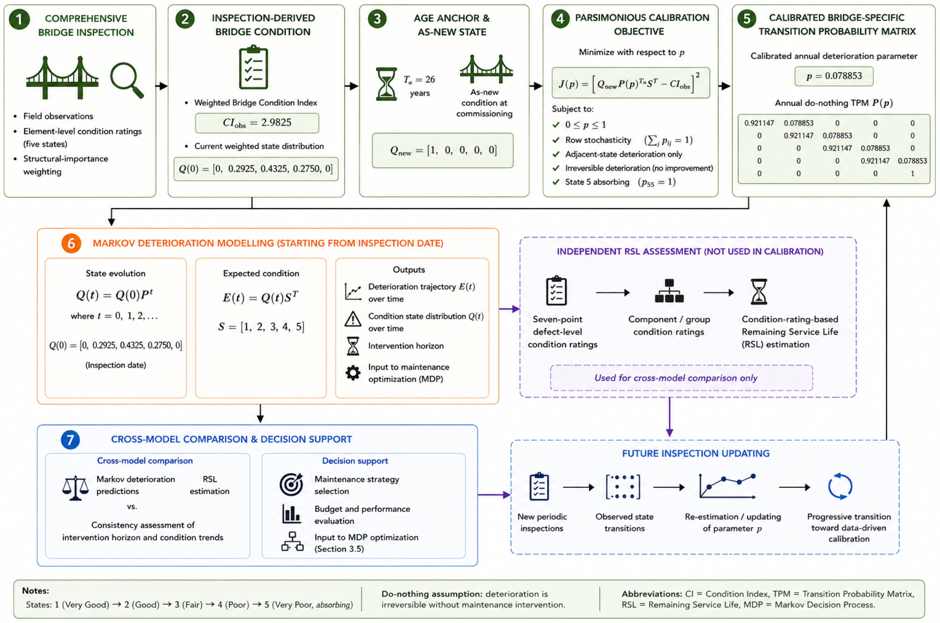
The known bridge age was then used as an explicit calibration anchor. Assuming an as-new condition at commissioning,

$$Q_{new}=\left[1 0 0 0 0\right]$$

the annual deterioration parameter was determined by minimizing the mismatch between the condition predicted at the inspection age and the observed Bridge Condition Index:

$$J(p)={\left[Q_{new}{P\left(p\right)}^{T_a}{S}^T-{CI}_{obs}\right]}^2$$

(5)

where $T_a$ = 26 years is the bridge age at inspection and ${CI}_{obs}$ = 2.9825 is the inspection-derived weighted Bridge Condition Index. The physically admissible parameter domain was restricted to 0 ≤ p ≤ 1, ensuring non-negative transition probabilities and preservation of row stochasticity. The calibration yielded $p$ = 0.078853, resulting in the bridge-specific annual do-nothing TPM

$$P\left(p\right)=\left[\begin{array}{ccccc}0.921147& 0.078853& 0& 0& 0\\ 0& 0.921147& 0.078853& 0& 0\\ 0& 0& 0.921147& 0.078853& 0\\ 0& 0& 0& 0.921147& 0.078853\\ 0& 0& 0& 0& 1\end{array}\right]$$

The calibrated model reproduces the observed Bridge CI at the known inspection age within numerical tolerance. The scalar calibration and final reproducibility check were performed in Python 3.12.13 (Python Software Foundation, Wilmington, DE, USA), using NumPy 2.3.5 for matrix operations and SciPy 1.17.0 (scipy.optimize.brentq) for root finding. The calibration equation was solved over the bracket 1 × 10⁻¹⁰ ≤ p ≤ 0.5; no user-defined starting value or multi-start procedure is required for this bracketed scalar solver. Solver tolerances and iteration limits were left at the library defaults. A numerical scan over the physical domain 0 ≤ p ≤ 1 confirmed that the age-26 expected condition is strictly increasing with p; within the numerical search bracket 1 × 10⁻¹⁰ ≤ p ≤ 0.5, a single root satisfies the calibration target, supporting uniqueness of the calibrated scalar solution under the adopted common-p model assumptions. Following calibration, the actual inspection-derived distribution,

$$Q\left(0\right)=\left[0 0.2925 0.4325 0.2750 0\right]$$

was used as the initial distribution for forward deterioration prediction from the inspection date. Importantly, the condition-rating-based Remaining Service Life (RSL) assessment described in Section 3.4 was not included in the TPM calibration objective; it was retained as an analytically independent engineering assessment for subsequent cross-model comparison.

The resulting TPM should therefore be interpreted as a parsimonious, bridge-specific engineering calibration under data scarcity rather than as a statistically estimated deterioration model. The single-bridge application is intended as a methodological demonstration of how an inspection-to-decision workflow can be established for an existing bridge with no historical condition record; it does not establish empirical transferability of the calibrated numerical parameters to other bridges. Such transferability requires validation across bridges of different structural types, ages, and exposure environments and, where available, comparison with longitudinal inspection records. As subsequent inspections of the investigated bridge become available, the engineering-calibrated parameter can be updated or replaced by observation-based transition estimates. The inspection-driven age-anchored calibration procedure is summarized in Figure 2.

3.4. Remaining Service Life Assessment

Although the inspection-driven Markov deterioration model provides a probabilistic prediction of future bridge condition, a complementary Remaining Service Life (RSL) assessment was also performed using the simplified condition-rating methodology proposed by Berk [29] and further developed by Caner et al. [28] for highway bridges without long-term periodic inspection records. This approach was specifically developed for bridge networks where historical inspection databases are unavailable, making advanced reliability-based service life prediction impractical. Under such circumstances, the current bridge condition and statistically derived deterioration trends provide a practical basis for estimating the RSL of the structure.

The method evaluates bridge performance using a seven-point condition-rating system, where a rating of 7 represents a bridge element in new condition, 5 indicates the onset of minor deterioration while preserving its intended function, 3 corresponds to the loss of the designed structural or functional performance and is regarded as the end-of-service threshold, and 1 denotes complete failure. Intermediate ratings of 6, 4, and 2 represent transitional condition levels between these principal ratings. Two additional codes, 8 and 9, are used for components that are not applicable to the bridge and components whose condition cannot be determined because of accessibility or other physical limitations, respectively; these codes do not represent additional deterioration states and are excluded from the computation of average condition ratings. Bridge elements are grouped into three functional categories: (i) main structural components, including the deck, girders, bearings, and piers; (ii) ground and earth-retaining components, including abutments, approach fills, and stabilization structures; and (iii) service components. The overall bridge condition rating is obtained using weighted averaging, in which the structural and ground component groups are assigned unit weighting factors, whereas service components receive a weighting factor of 0.5 to reflect their comparatively smaller influence on structural safety. This weighting strategy was originally established through engineering experience and adopted in the service life methodology.

The overall bridge condition rating is computed as

$$CR={\displaystyle \frac{({CR}_{main}\cdot 1.0+{CR}_{ground}\cdot 1.0+{CR}_{service}\cdot 0.5)}{2.5}}$$

(6)

where ${CR}_{main}$, ${CR}_{ground}$ and ${CR}_{service}$ denote the average condition ratings of the main structural, ground, and service component groups, respectively.

Assuming approximately linear deterioration behavior, the RSL is estimated as

$$RSL={\displaystyle \frac{\left(CR-3\right)}{DR}}$$

(7)

where $DR$ is the annual deterioration rate and the condition rating of 3 represents the limit at which the bridge is considered to have lost its intended service function. Based on statistical evaluations of comparable Turkish highway bridges, deterioration rates of 0.0403 year⁻¹, 0.0227 year⁻¹, 0.0353 year⁻¹, and 0.0319 year⁻¹ have been reported for the main structural components, ground components, service components, and the overall bridge, respectively, whereas the average deterioration trend reported for OECD bridge inventories is approximately 0.025 year⁻¹. These values provide the deterioration reference required for the simplified RSL estimation.

Although the Markov deterioration model and the RSL assessment are both informed by the same field inspection, they employ distinct condition representations for different analytical purposes. The harmonized five-state system described in Section 3.2 defines the state space used for probabilistic Markov deterioration modelling, whereas the Berk–Caner methodology [28,29] independently evaluates the observed defects using its original seven-point condition-rating scale for service-life estimation. Accordingly, no numerical state-to-state conversion was performed between the five-state Markov system and the seven-point RSL scale. Rather, the observed inspection evidence was evaluated separately within the respective condition framework of each method. As noted above, ratings of 8 and 9 in the RSL methodology are non-condition codes and were excluded from the calculation of average condition ratings. For transparency and reproducibility, the complete defect/check-item ratings, excluded non-condition codes, and element- and group-level averaging calculations used in the condition-rating-based RSL assessment are provided in Appendix A (

Table A2. Element-level condition-rating scores and averaging calculations used in the RSL assessment.

Group	Element	Included Defect/Check-Item Ratings	Excluded Code	Element CR
Main Structural	Deck slab	6, 5, 5, 6, 4	-	5.20
Main Structural	Steel girders	6, 6, 4, 5, 5	-	5.20
Main Structural	Elastomeric bearings	6, 4, 5, 6	-	5.25
Main Structural	Pier columns	3, 3, 3, 3, 5, 5	9	3.67
Ground/soil-retaining	Abutments	4, 5, 3, 3, 5, 5, 3	-	4.00
Ground/soil-retaining	Approach fill	6, 6, 6	-	6.00
Ground/soil-retaining	Slope stabilization	6, 5, 5	-	5.33
Service	Wearing surface	6, 6, 5, 5	-	5.50
Service	Steel railings	7, 5, 7	-	6.33
Service	Concrete curb	5, 6, 7	-	6.00
Service	Drainage system	4, 7, 6	-	5.67
Service	Expansion joints	6, 3, 5, 5, 6, 6	-	5.17

Note: CR values were calculated as arithmetic means of the applicable defect/check-item ratings. Code 9 denotes an inaccessible or indeterminate condition and was excluded from averaging. Steel railings and concrete curbs were combined into a single railing/curb service-element value before calculation of the service-group mean. The resulting unrounded group ratings were CR_main = 4.829167, CR_ground = 5.111111, and CR_service = 5.625000. Equation (6) gives an overall bridge rating of CR = 5.101111. Values in the main results tables are rounded to two decimal places.

).

Importantly, the condition-rating-based RSL assessment was not used as a calibration target or constraint in the Markov deterioration model described in Section 3.3. The two approaches were maintained analytically independent. The Markov model provides a probabilistic prediction of future bridge-condition evolution and the associated intervention horizon, whereas the condition-rating method provides an engineering estimate of RSL from the independently assigned seven-point ratings and externally established deterioration rates. Their results are therefore compared in Section 4 at the level of predicted time horizons as an independent cross-model consistency check, rather than through direct equivalence of their condition-state scales or as a formal validation of either model.

3.5. Markov Decision Process for Maintenance Optimization

The inspection-driven deterioration model presented in Section 3.3 predicts the probabilistic evolution of bridge condition under the do-nothing scenario, while the independent RSL assessment described in Section 3.4 provides a complementary condition-based estimate of the remaining service-life horizon. However, neither approach determines which maintenance action should be implemented or when intervention should be undertaken. To convert deterioration prediction into maintenance decisions, the calibrated bridge-specific Markov deterioration model was integrated into a discrete-time Markov Decision Process (MDP). The MDP identifies condition- and time-dependent maintenance policies by jointly considering stochastic deterioration, maintenance effects, intervention costs, and long-term condition consequences within a unified optimization framework [30,31,32,34,35].

The MDP is defined as

$$M=\left\{S,A,P^a,C,\gamma ,T\right\}$$

(8)

where S is the set of bridge condition states, A is the set of feasible maintenance actions, P^a denotes the action-dependent TPMs, C is the one-period cost function, γ is the discount factor, and T is the finite planning horizon. A one-year decision interval was adopted to maintain consistency with the annual deterioration model described in Section 3.3.

3.5.1. Condition States and Maintenance Actions

The MDP employs the harmonized five-state bridge condition assessment framework introduced in Section 3.2,

$$S=\left\{1,2,3,4,5\right\}$$

thereby ensuring consistency among inspection-based condition assessment, Markov deterioration modelling, and maintenance optimization. The five-state representation provides sufficient resolution to distinguish progressive deterioration and corresponding intervention levels while maintaining a compact and interpretable state space for stochastic deterioration modelling and dynamic maintenance decision-making.

The MDP is formulated as a representative condition-state decision model rather than as a joint physical-state model of the entire bridge or a separate multi-component MDP. Its state variable denotes the condition class to which an assessed element category is assigned, and the optimized policy maps each condition state to the corresponding maintenance-action class at each decision epoch. The bridge-level condition distribution is used to evaluate the expected trajectory and cost of this state-dependent policy. For practical interpretation, the resulting condition–action mapping is subsequently applied to each assessed element category according to its inspection-derived condition state; this does not imply that a separate element-specific optimization problem was solved for every physical bridge component.

Four maintenance actions representing progressively increasing intervention levels were considered,

$$A=\left\{A_0,A_1,A_2,A_3\right\}$$

where A₀ denotes do nothing/routine monitoring, A₁ preventive maintenance, A₂ corrective repair, and A₃ major rehabilitation. The maintenance actions and their typical engineering applications are summarized in

Table 3. Maintenance actions adopted in the MDP model.

Action	Maintenance Level	Description	Typical Applications
A0	Do nothing/monitoring	No physical intervention; the element continues to deteriorate according to the do-nothing transition matrix	Visual monitoring and periodic inspection
A1	Preventive maintenance	Minor intervention intended to arrest or slow early-stage deterioration	Drainage cleaning, joint sealing, crack sealing, protective coating, local patching
A2	Corrective repair	Repair intended to restore a moderately or severely deteriorated element to an improved condition state	Concrete repair, reinforcement treatment, bearing-seat repair, joint replacement and local strengthening
A3	Major rehabilitation	Comprehensive intervention that substantially restores structural or functional performance	Extensive pier rehabilitation, cap-beam strengthening, bearing replacement, scour protection and structural rehabilitation

.

To avoid technically impractical or economically unrealistic decisions, the feasible action set was restricted according to the current bridge condition state,

$$A\left(1\right)=\left\{A_0\right\};\hspace{0.25em}A\left(2\right)=\{A_0,A_1\};\hspace{0.25em}A\left(3\right)=\{A_0,A_1,A_2\};\hspace{0.25em}A\left(4\right)=\{A_0,A_2,A_3\};\hspace{0.25em}A\left(5\right)=\{A_0,A_3\}$$

(9)

reflecting the engineering principle that preventive maintenance is most appropriate during the early stages of deterioration, whereas advanced deterioration generally requires corrective repair or major rehabilitation.

3.5.2. Action-Dependent Transition Models

The action-dependent transition models describe the influence of maintenance interventions on the stochastic evolution of bridge condition. The bridge-specific TPM calibrated through the inspection-driven procedure described in Section 3.3 was adopted as the baseline transition model for the do-nothing action, A₀. Accordingly, P^A₀ represents the expected annual deterioration process in the absence of physical intervention and is given by

$$P^{A_0}=\left[\begin{array}{ccccc}0.921147& 0.078853& 0& 0& 0\\ 0& 0.921147& 0.078853& 0& 0\\ 0& 0& 0.921147& 0.078853& 0\\ 0& 0& 0& 0.921147& 0.078853\\ 0& 0& 0& 0& 1\end{array}\right]$$

The remaining action-dependent transition matrices were formulated as engineering-based maintenance-effect models representing the expected relative effects of preventive maintenance, corrective repair, and major rehabilitation. Because bridge-specific post-maintenance inspection histories were unavailable, these matrices were not statistically calibrated from observed intervention outcomes. They should therefore be interpreted as structured engineering assumptions used to evaluate alternative maintenance strategies within the decision-support framework.

A common condition-state transition structure was applied across the heterogeneous element categories because element-type-specific longitudinal deterioration and post-maintenance records were unavailable. This assumption does not imply that steel, reinforced-concrete, bearing, pavement, drainage, and other bridge components deteriorate or respond to maintenance at identical physical rates. It is a deliberate screening-level simplification that enables a transparent state-based decision model to be implemented under the available data conditions. The resulting transition matrices and optimized policy should therefore be interpreted as category-level decision-support representations rather than empirically identified element-specific deterioration and intervention-response models. As element-specific inspection histories become available, separate transition and maintenance-effect matrices can be introduced without changing the overall MDP architecture.

Preventive maintenance, A₁, was represented as an intervention primarily intended to slow deterioration and, where applicable, provide limited improvement in condition:

$$P^{A_1}=\left[\begin{array}{ccccc}1.00& 0.00& 0.00& 0.00& 0.00\\ 0.20& 0.75& 0.05& 0.00& 0.00\\ 0.00& 0.25& 0.65& 0.10& 0.00\\ 0.00& 0.00& 0.30& 0.60& 0.10\\ 0.00& 0.00& 0.00& 0.20& 0.80\end{array}\right]$$

Corrective repair, A₂, was represented by a stronger restorative effect, with increased probabilities of transition toward improved condition states:

$$P^{A_2}=\left[\begin{array}{ccccc}1.00& 0.00& 0.00& 0.00& 0.00\\ 0.70& 0.30& 0.00& 0.00& 0.00\\ 0.10& 0.75& 0.15& 0.00& 0.00\\ 0.00& 0.15& 0.75& 0.10& 0.00\\ 0.00& 0.00& 0.30& 0.60& 0.10\end{array}\right]$$

Major rehabilitation, A₃, was represented as the strongest intervention, with a high probability of restoring deteriorated components to good or very good condition:

$$P^{A_3}=\left[\begin{array}{ccccc}0.95& 0.05& 0.00& 0.00& 0.00\\ 0.90& 0.09& 0.01& 0.00& 0.00\\ 0.85& 0.14& 0.01& 0.00& 0.00\\ 0.85& 0.14& 0.01& 0.00& 0.00\\ 0.85& 0.14& 0.01& 0.00& 0.00\end{array}\right]$$

Each action-dependent transition matrix satisfies the stochastic requirement that the probabilities in every row sum to unity. The maintenance-effect matrices were constructed to preserve three engineering constraints: (i) intervention effectiveness increases from preventive maintenance to corrective repair and major rehabilitation; (ii) no intervention is assumed to provide deterministic restoration, thereby retaining residual deterioration and intervention-performance uncertainty; and (iii) the resulting transition structure remains physically interpretable within the five-state condition framework.

Because P^A₁, P^A₂, and P^A₃ are engineering-based rather than empirically calibrated post-maintenance transition models, their influence on the resulting maintenance decisions was explicitly examined through the sensitivity analysis described in Section 3.5.6. Accordingly, the optimization results should be interpreted as decision-support outcomes conditional on the adopted maintenance-effect assumptions rather than as uniquely identified bridge-specific intervention-response probabilities. As future post-maintenance inspection records become available, these matrices can be progressively updated or statistically recalibrated without altering the overall MDP formulation.

3.5.3. Cost Structure and Optimization Objective

The maintenance optimization problem was formulated to minimize the expected cumulative discounted life-cycle cost over the finite planning horizon while maintaining acceptable bridge condition. For a bridge in condition state s subjected to maintenance action a, the one-period cost was defined as

$$C\left(s,a\right)=C_M\left(a\right)+C_S\left(s\right)$$

(10)

where C_M(a) denotes the normalized direct cost associated with maintenance action a, and C_S(s) represents the condition-state penalty associated with deterioration-related loss of serviceability, increasing intervention urgency, and adverse consequences of remaining in deteriorated states.

Because bridge maintenance expenditures vary substantially among agencies, geographical regions, traffic conditions, economic environments, and management practices, normalized dimensionless cost coefficients were adopted instead of project-specific monetary values, consistent with their use in bridge management and MDP-based infrastructure optimization studies [30,31,35,47]. The resulting objective therefore represents a relative decision-support metric rather than an estimate of actual construction expenditure or monetary savings. This formulation enables alternative maintenance strategies to be compared consistently under identical modelling assumptions while avoiding unsupported site-specific monetary estimates.

The normalized maintenance-action costs were assigned as $C_M\left(A_0\right)=0$, $C_M\left(A_1\right)=2$, $C_M\left(A_2\right)=8$, and $C_M\left(A_3\right)=20$, representing the increasing resource requirements associated with do nothing/routine monitoring, preventive maintenance, corrective repair, and major rehabilitation, respectively. The corresponding condition-state penalties were assigned as $C_S\left(1\right)=0$, $C_S\left(2\right)=1$, $C_S\left(3\right)=4$, $C_S\left(4\right)=12$, and $C_S\left(5\right)=30$. Their nonlinear increase reflects the progressively greater serviceability loss, intervention urgency, operational concern, and consequences associated with advanced deterioration.

In particular, the relatively high penalty assigned to State 5 represents the combined consequence of allowing the bridge to remain in a critical condition requiring urgent intervention. Accordingly, a separate failure-cost term was not introduced into the executable cost function; the critical-condition consequence is incorporated directly within $C_S\left(5\right)$. This formulation maintains consistency between the mathematical description and the computational implementation of the MDP.

The adopted normalized cost structure preserves the economic hierarchy

$$C_M\left(A_0\right)<C_M\left(A_1\right)<C_M\left(A_2\right)<C_M\left(A_3\right)$$

(11)

while the convex increase in condition-state penalties discourages policies that defer intervention until severe deterioration occurs. The coefficients should therefore be interpreted as engineering decision parameters that preserve relative intervention and deterioration consequences rather than as actual agency expenditures. For practical implementation, the normalized coefficients can be replaced by agency-specific monetary values, including maintenance, inspection, traffic-management, user-delay, and other relevant consequence costs, without changing the structure of the optimization framework.

A baseline annual real discount rate of 3% was adopted, corresponding to a discount factor of

$$\mathsf{\gamma }={\displaystyle \frac{1}{1+0.03}}\cong 0.9709$$

(12)

The baseline optimization was conducted over a 50-year finite planning horizon. Because the normalized cost coefficients, discount rate, and planning horizon are modelling assumptions rather than bridge-specific observations, their influence on the resulting maintenance decisions was explicitly examined through the sensitivity analyses described in Section 3.5.6. The baseline normalized cost coefficients used in the MDP are summarized in

Table 4. Baseline normalized cost coefficients adopted in the MDP model.

Condition State	State Penalty CS(s)	Maintenance Action	Action Cost CM(a)
1	0	A0: Do nothing/monitoring	0
2	1	A1: Preventive maintenance	2
3	4	A2: Corrective repair	8
4	12	A3: Major rehabilitation	20
5	30

Note: The normalized cost coefficients are dimensionless engineering decision parameters adopted to preserve the relative economic hierarchy of maintenance interventions and the increasing consequences of deterioration. The State 5 penalty incorporates the critical-condition consequence within the state-cost structure; no separate failure-cost term is used in the computational model. These coefficients are intended for relative methodological comparison rather than direct estimation of construction expenditure and may be replaced by agency-specific monetary values without altering the optimization framework.

.

3.5.4. Dynamic Programming Solution

The optimal maintenance policy was determined using finite-horizon dynamic programming based on the Bellman optimality principle. The optimization minimizes the expected cumulative discounted normalized cost over the 50-year planning horizon while accounting for the current bridge condition, the feasible maintenance actions in each state, and the action-dependent transition probabilities defined in Section 3.5.2. A one-year decision interval was adopted, consistent with the annual deterioration process used throughout the framework. Accordingly, the 50-year horizon comprises 50 maintenance decision periods, t = 0, …, 49, followed by the terminal condition assessment at t = 50; no additional maintenance action is assigned at the terminal epoch.

Let $V_t\left(s\right)$ denote the minimum expected cumulative discounted cost from decision year t to the end of the planning horizon when the bridge is in condition state s. For t = T−1, …, 0, the finite-horizon Bellman recursion is

$$V_t\left(s\right)=\underset{a\in A\left(s\right)}{\mathrm{m}\mathrm{i}\mathrm{n}}\left[C\left(s,a\right)+\gamma \sum _{s^{\prime }\in S}{P}_{s{s}^{\prime }}^a{V}_{t+1}\left(s^{\prime }\right)\right], {\mathrm{V}}_T\left(s\right)=C_S\left(s\right)$$

(13)

where $A\left(s\right)$ is the set of feasible maintenance actions for state s, $C\left(s,a\right)$ is the normalized one-period cost defined in Equation (10), $P_{s{s}^{\prime }}^a$ is the probability of transition from state s to state s′ under action a, $\gamma$ is the annual discount factor, and T = 50 years is the finite planning horizon. The terminal value ${\mathrm{V}}_T\left(s\right)=C_S\left(s\right)$ applies the condition-state penalty at the end of the 50-year planning horizon without assigning an additional maintenance action, thereby maintaining consistency with the implemented finite-horizon cost calculation.

The recursion was solved by backward induction, beginning at the terminal year and proceeding sequentially to the initial decision year. At each state and decision epoch, all feasible actions were evaluated and the action yielding the minimum expected discounted cost was selected. The resulting time-dependent optimal policy is therefore

$${\mathsf{\pi }}_t^{*}\left(s\right)=\underset{a\in A\left(s\right)}{\begin{array}{cc}arg& min\end{array}}\left[C\left(s,a\right)+\gamma \sum _{s^{\prime }\in S}{P}_{s{s}^{\prime }}^a{V}_{t+1}\left(s^{\prime }\right)\right]$$

(14)

Unlike an infinite-horizon stationary formulation, the finite-horizon solution permits the optimal action for a given condition state to depend on the remaining planning period. Accordingly, the optimized maintenance strategy was evaluated from the bridge-specific initial condition distribution and propagated over the 50-year horizon using the corresponding action-dependent transition matrices. This procedure provides both the expected condition trajectory and the discounted normalized life-cycle cost associated with the optimized policy, enabling direct comparison with the benchmark maintenance strategies described in Section 4.

3.5.5. Computational Implementation

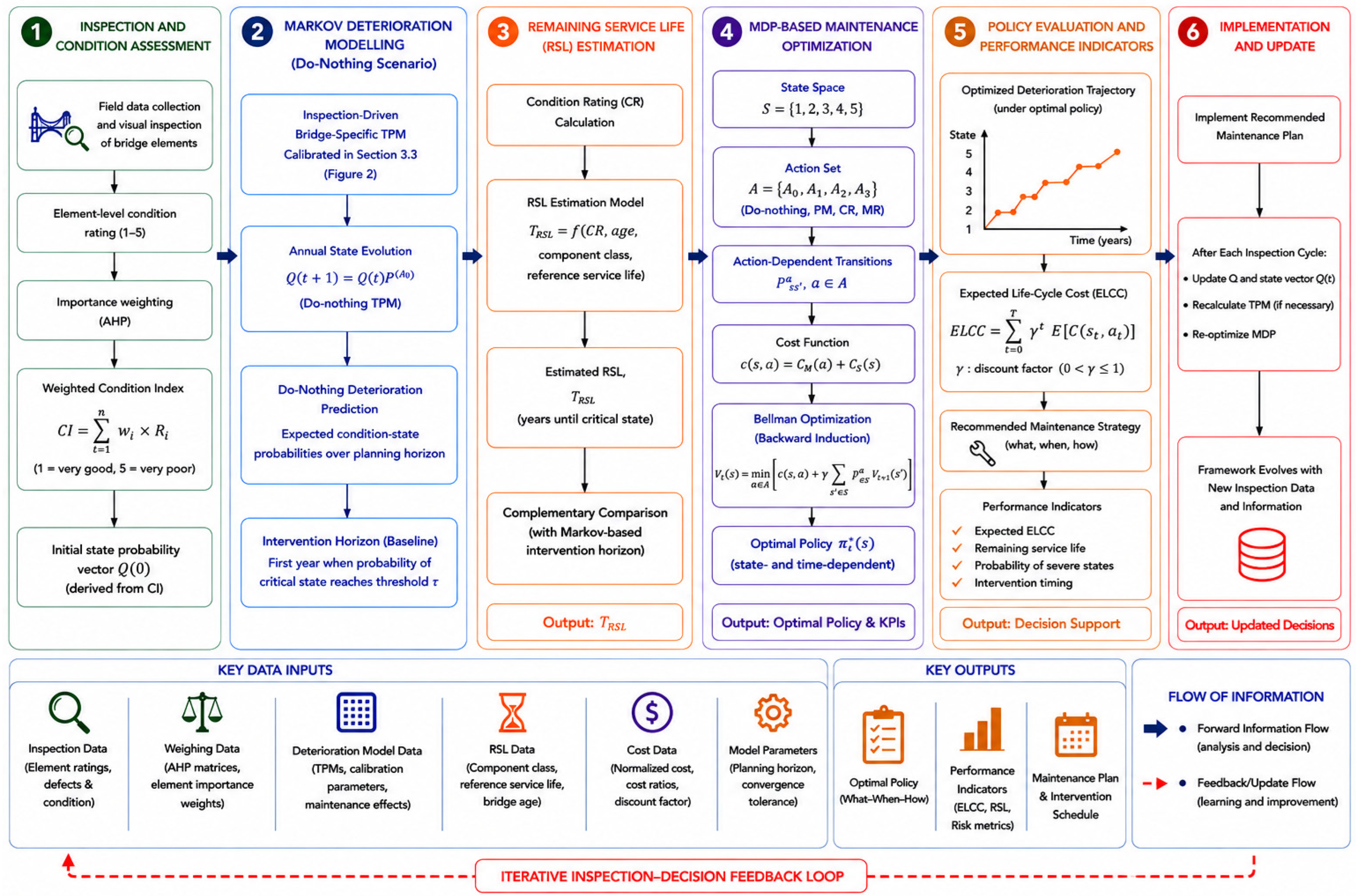
The proposed decision-support framework integrates the methodological components described in the preceding sections into a unified computational workflow for bridge condition assessment, deterioration prediction, remaining service life (RSL) assessment, and maintenance optimization. Inspection observations are first converted into element-level condition states and aggregated using the importance-weighting procedure described in Section 3.2. The resulting bridge condition information defines the initial state distribution for the inspection-driven Markov deterioration model developed in Section 3.3.

Two complementary prognostic paths are subsequently employed. The calibrated bridge-specific Markov model propagates the five-state condition distribution under the do-nothing scenario and provides the probabilistic deterioration trajectory used in the maintenance optimization framework. In parallel, the condition-rating-based procedure described in Section 3.4 provides an independent engineering estimate of RSL. The latter is not used to calibrate the Markov transition probabilities or to define the MDP state space; rather, it provides a complementary service-life estimate that can be compared with the intervention horizon inferred from the Markov deterioration prediction.

For maintenance optimization, the calibrated do-nothing transition probability matrix is combined with the engineering-based action-dependent transition models, feasible action sets, and normalized cost structure defined in Section 3.5.1, Section 3.5.2 and Section 3.5.3. The resulting finite-horizon MDP is solved over a 50-year planning horizon by backward induction according to Equation (13). The finite-horizon MDP was implemented in Python using NumPy-based array and matrix operations; at each decision year and condition state, all feasible actions were evaluated directly and the minimum-cost action was selected, so no iterative optimization solver or convergence tolerance was required. At each annual decision epoch, the model determines the state- and time-dependent action that minimizes the expected cumulative discounted normalized cost. Propagation of the condition-state probabilities under the resulting policy provides the optimized deterioration trajectory and the associated decision-performance indicators.

The overall computational workflow is illustrated in Figure 3.

The framework is deliberately modular: condition assessment, deterioration modelling, RSL assessment, maintenance-effect assumptions, cost parameters, and optimization settings can be independently updated as new inspection or maintenance information becomes available. Following subsequent inspection cycles, the condition assessment can therefore be updated and, where sufficient evidence becomes available, the deterioration and maintenance-effect models can be recalibrated before the maintenance policy is re-optimized. This iterative architecture is particularly relevant to bridges with limited or no historical inspection records because the initial engineering-informed model can progressively evolve toward a data-supported bridge-specific decision model.

3.5.6. Sensitivity and Uncertainty Analysis

To evaluate the robustness of the proposed maintenance optimization framework to the principal engineering and modelling assumptions, a series of scenario-based sensitivity analyses was performed. The examined parameters included the normalized maintenance-action costs, condition-state penalties, engineering-based maintenance-effect transition probabilities, discount rate, planning horizon, do-nothing deterioration intensity, and the structural shape of the transition probability matrix (TPM). These parameters influence either the finite-horizon maintenance decisions, the predicted deterioration trajectory, or the associated life-cycle performance indicators.

First, the normalized maintenance-action costs and condition-state penalties were examined in separate scenario groups. Within the maintenance-cost scenarios, all nonzero action costs, $C_M\left(A_1\right)$, $C_M\left(A_2\right)$, and $C_M\left(A_3\right)$, were scaled collectively to 0.8 and 1.2 times their baseline values, while $C_M\left(A_0\right)$ = 0 remained unchanged. Within the state-penalty scenarios, all nonzero penalties, $C_S\left(2\right)$–$C_S\left(5\right)$, were likewise scaled collectively to 0.8 and 1.2 times their baseline values, while $C_S\left(1\right)$ = 0 remained unchanged. Thus, the coefficients within each parameter group were not perturbed individually; each group was scaled collectively while preserving the baseline action-cost and deterioration-severity hierarchies. For every scenario, the finite-horizon MDP and the corresponding matched do-nothing solution were recomputed.

Second, maintenance-effect sensitivity was evaluated by scaling the improvement probabilities in the preventive-maintenance, corrective-repair, and major-rehabilitation transition matrices. Using row i for the current state and column j for the next state, the below-diagonal entries with j < i represent transitions to improved condition states. Here, ${\mathrm{P}}^{\mathrm{P}\mathrm{M}}={\mathrm{P}}_{{\mathrm{A}}_1}$, ${\mathrm{P}}^{\mathrm{C}\mathrm{R}}={\mathrm{P}}_{{\mathrm{A}}_2}$, and ${\mathrm{P}}^{\mathrm{M}\mathrm{R}}={\mathrm{P}}_{{\mathrm{A}}_3}$ denote the preventive-maintenance, corrective-repair, and major-rehabilitation transition matrices defined in Section 3.5.2, respectively; their entries correspond to the action-dependent transition probabilities $P_{s{s}^{\prime }}^a$ used in the Bellman recursion in Equation (13). The entries varied were $P_{21}^{PM}$, $P_{32}^{PM}$, $P_{43}^{PM}$, and $P_{54}^{PM}$; $P_{21}^{CR}$, $P_{31}^{CR}$, $P_{32}^{CR}$, $P_{42}^{CR}$, $P_{43}^{CR}$, $P_{53}^{CR}$, and $P_{54}^{CR}$; and $P_{21}^{MR}$, $P_{31}^{MR}$, $P_{32}^{MR}$, $P_{41}^{MR}$, $P_{42}^{MR}$, $P_{51}^{MR}$, and $P_{52}^{MR}$. These improvement probabilities were multiplied collectively by factors of 0.8 and 1.2 in the reduced- and increased-effectiveness scenarios, respectively. Entries representing deterioration to poorer states (j > i) were left unchanged. After perturbation, the diagonal entry of each affected row was set equal to one minus the sum of its off-diagonal entries. If the 1.2 scaling caused the total improvement probability to exceed the probability mass available after retaining the poorer-state transitions, the total improvement probability was capped at that available mass and its original distribution among the improved states was preserved proportionally. This procedure maintained non-negativity and unit row sums. The resulting matrices were also checked to preserve the relative intervention-effectiveness hierarchy among preventive maintenance, corrective repair, and major rehabilitation. The finite-horizon MDP was then re-solved using each perturbed matrix set.

Third, the influence of the economic discounting assumption was evaluated by varying the annual real discount rate from 1% to 5%, with 3% adopted as the baseline value. For each discount-rate scenario, the finite-horizon MDP was re-evaluated using the same state space, feasible-action structure, transition models, cost formulation, and planning horizon. This allows the effect of alternative long-term economic perspectives on the timing and selection of maintenance interventions and on the expected discounted life-cycle cost to be assessed consistently.

Additional scenarios were used to examine the effects of the planning horizon and uncertainty in the deterioration-model assumptions. The planning horizon was varied between 25 and 75 years relative to the 50-year baseline, while the do-nothing deterioration intensity was scaled to 0.8 and 1.2 times its baseline level. The structural form of the do-nothing TPM was also stress-tested using alternative state-dependent deterioration patterns while preserving non-negativity, row stochasticity, and the monotonic deterioration structure. These scenarios were intended to assess model-form robustness rather than to represent statistically estimated parameter distributions.

For each sensitivity scenario, the finite-horizon MDP was re-solved and the resulting optimized discounted cost, cost reduction relative to the corresponding do-nothing solution, expected condition and State-1 probability at Year 16, initial optimal policy, and policy agreement over Years 0–12 were compared with the baseline solution. The sensitivity analysis was interpreted as an engineering scenario-based robustness assessment rather than as a statistical uncertainty or confidence analysis.

The adopted OAT procedure should therefore be interpreted as a first-order robustness assessment rather than a full probabilistic uncertainty quantification. The present study does not assign probability distributions to the maintenance-effect parameters or cost coefficients and does not propagate their joint uncertainty through the optimization model. Such analyses would require additional empirical information that is not available for the investigated bridge. As repeated inspection and post-maintenance observations become available, the modular framework can accommodate more formal uncertainty treatments, including probabilistic parameter sampling, Monte Carlo propagation, or Bayesian updating of deterioration and maintenance-effect parameters. The results of the present sensitivity analyses and their implications for the stability of the maintenance recommendations are presented in Section 4.

4. Results and Discussion

4.1. Inspection Findings and Element Condition States

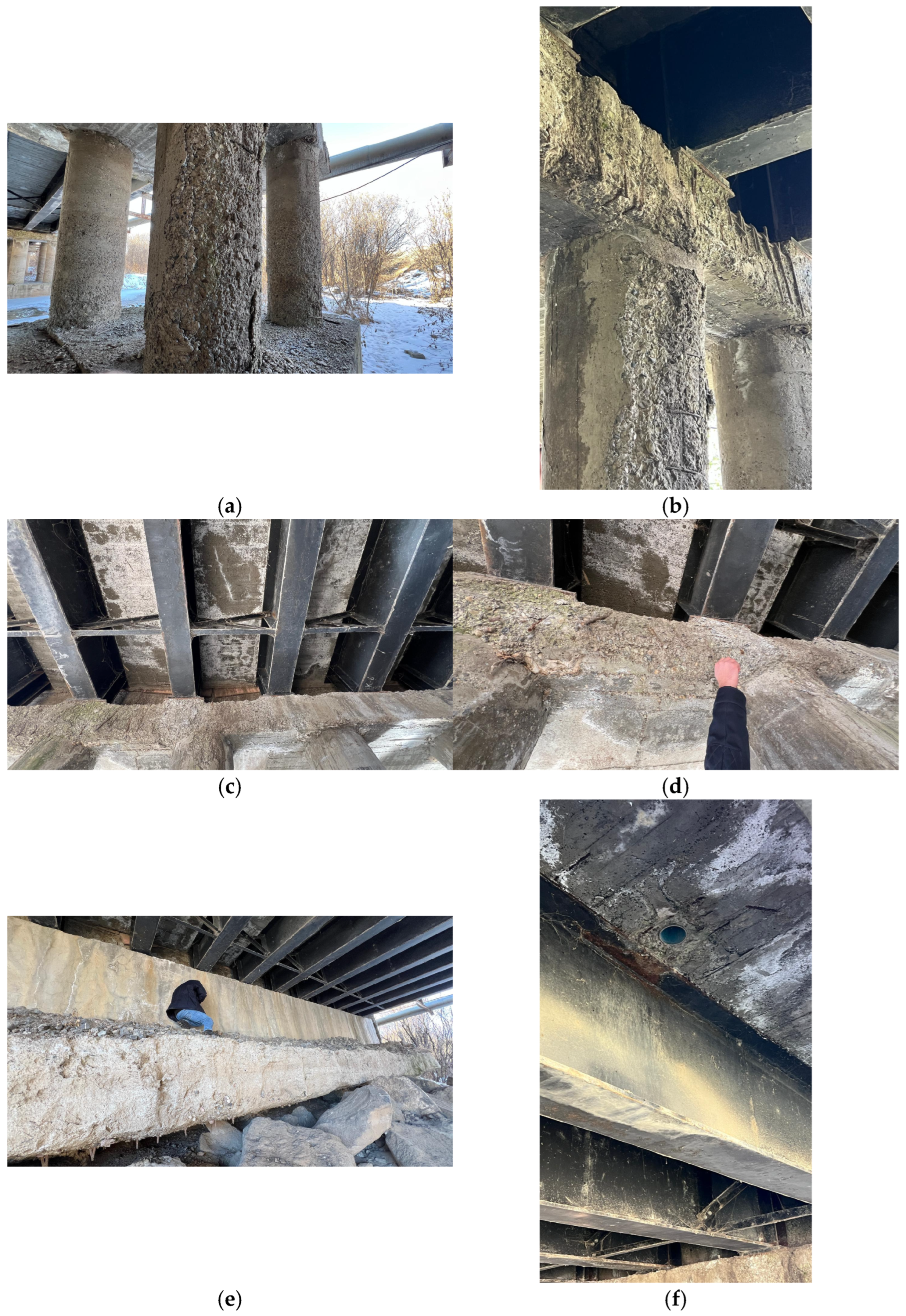
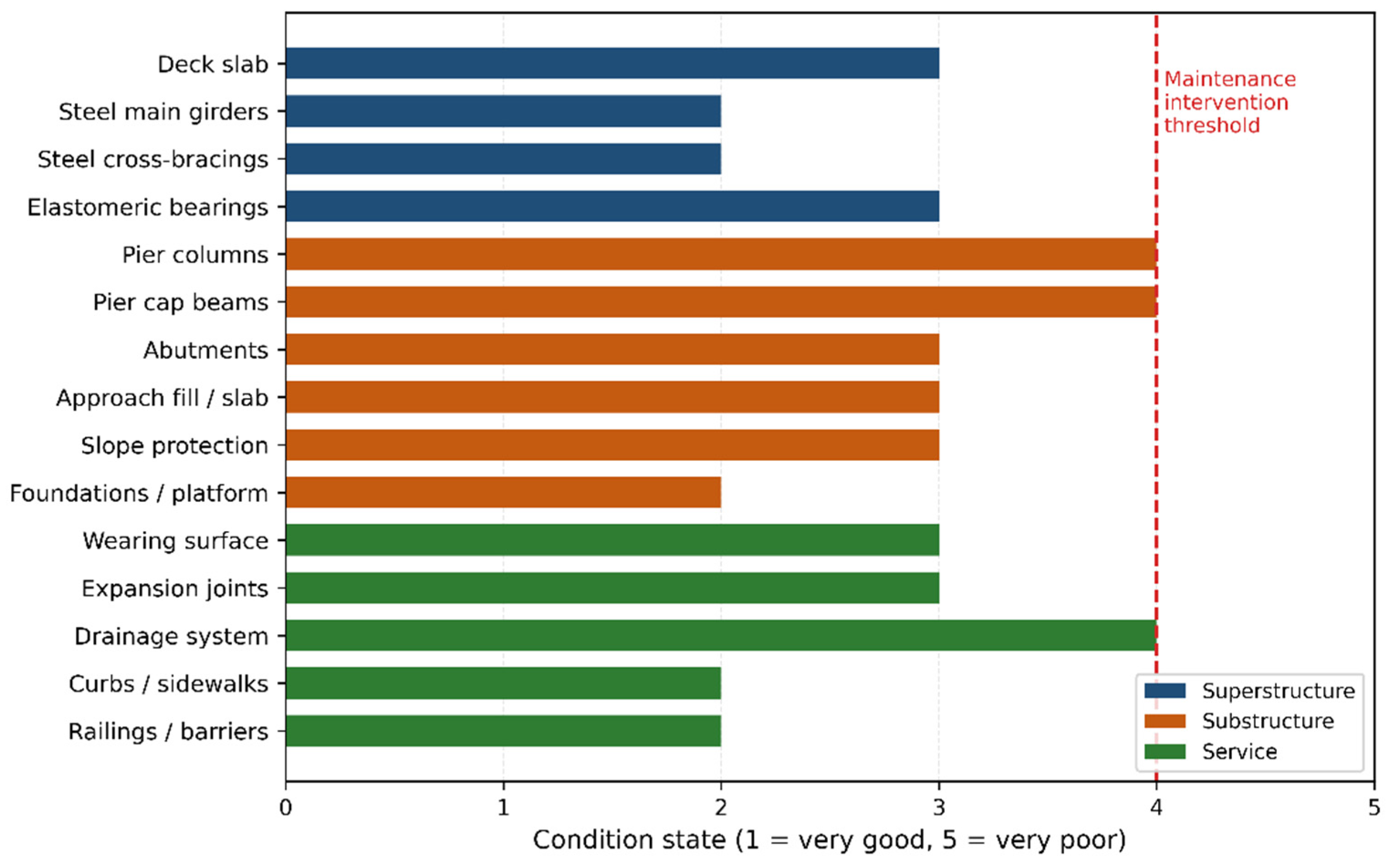
The consolidated inspection results are summarized in

Table 5. Element-level damage observations, condition states, and bridge-level weights.

Group	Element	Principal Observed Damage	State	Weight (Bridge)
Superstructure	Deck slab	Moisture/leakage traces, efflorescence, local cracks, reinforcement exposure	3	0.1050
Superstructure	Steel main girders	Paint loss, local superficial corrosion, oxidation near bearings	2	0.1225
Superstructure	Steel cross-bracings	Soiling, local rust, superficial corrosion at connections	2	0.0525
Superstructure	Elastomeric bearings	Wide cracks and concrete disintegration at bearing seats, moisture	3	0.0700
Substructure	Pier columns	Cover loss, exposed/corroded reinforcement, section loss, long cracks	4	0.1350
Substructure	Pier cap beams	Advanced spalling, segregation, exposed reinforcement cage, leakage	4	0.0900
Substructure	Abutments	Surface deterioration, delamination, suspected scour/void at west abutment	3	0.0900
Substructure	Approach fill/slab	Irregular surface, material loss, suspected voids near abutments	3	0.0338
Substructure	Slope protection	Displaced riprap, slope degradation by river action, scour risk	3	0.0338
Substructure	Foundations/platform	No visible settlement or rotation; water action and debris present	2	0.0675
Service	Wearing surface	Cracks, patches, local raveling, surface deterioration	3	0.0500
Service	Expansion joints	Surface discontinuity, longitudinal crack lines, probable loss of function	3	0.0500
Service	Drainage system	Inadequate discharge, widespread leakage and moisture under deck	4	0.0500
Service	Curbs/sidewalks	Superficial deterioration, cracking, local delamination	2	0.0250
Service	Railings/barriers	Paint loss, local corrosion; structural continuity preserved	2	0.0250

, representative damage observations are presented in Figure 4, and the element-level condition-state distribution is illustrated in Figure 5. The most severe deterioration was observed in the pier columns and pier cap beams, both classified as State 4. These elements exhibited extensive concrete cover loss, severe segregation, exposed and corroded reinforcement with local section loss, and longitudinal cracking, indicating advanced deterioration of the reinforced-concrete substructure. In addition, rounded river gravel observed within some spalled concrete fragments may indicate unfavorable aggregate characteristics that could have contributed to the observed material degradation.

The deck slab was classified as State 3 because of widespread moisture traces, efflorescence, calcium deposits, local cracking, and reinforcement exposure. The steel main girders and cross-bracings remained in comparatively good observed condition (State 2), exhibiting primarily localized coating deterioration and superficial corrosion, whereas the elastomeric bearing regions were assigned State 3 because of cracking and concrete deterioration around the bearing seats. These observations indicate that the most advanced visible deterioration is concentrated in the reinforced-concrete substructure, while the steel superstructure exhibits comparatively limited observable deterioration under the current exposure conditions.

The western abutment exhibited displaced riprap and indications consistent with possible local scour, leaving portions of the footing protection locally deficient despite the presence of deep foundation piles. Because the foundation and underwater conditions could not be fully observed during the inspection, the presence and extent of scour should be verified through a dedicated hydraulic and substructure investigation. The drainage system was classified as State 4 because inadequate scupper geometry allows runoff to discharge directly onto the steel girders and substructure instead of being effectively conveyed away from the bridge. Persistent moisture, together with leakage through deteriorated expansion-joint lines, exposes the deck soffit, bearing regions, and cap beams to repeated wetting and was therefore identified as a major deterioration pathway. Overall, the inspection indicates that the observed deterioration is governed primarily by moisture-related mechanisms and localized substructure deficiencies, establishing the engineering basis for the subsequent condition assessment, deterioration modelling, and maintenance optimization.

4.2. Weighted Bridge Condition Index

To integrate the element-level condition states into a single bridge-level indicator, importance weights were assigned according to each component’s structural function, contribution to load transfer, redundancy, potential consequences of failure, and influence on bridge serviceability, following established Bridge Management System (BMS) principles [2,4,5,7,43]. Reflecting these engineering considerations, group-level weighting factors of 0.35, 0.45, and 0.20 were assigned to the superstructure, substructure, and service components, respectively. Within each group, element weights were distributed according to their relative structural and functional significance. Consequently, the pier columns and pier cap beams received the highest weights within the substructure because of their direct role in the vertical load-transfer system, whereas the drainage system received the highest service-component weight because of its influence on moisture-related deterioration of adjacent bridge elements. The complete element-level weighting scheme is presented in Table 5.

Application of the weighted condition assessment procedure described in Section 3.2 yielded an overall CI of 2.9825 (≈2.98), with subsystem indices of 2.50, 3.35, and 3.00 for the superstructure, substructure, and service components, respectively. The resulting bridge-level index corresponds to State 3 (moderate condition). However, the presence of State 4 deterioration in the pier columns, pier cap beams, and drainage system demonstrates that maintenance priorities cannot be determined from the global bridge condition alone. These locally advanced deterioration states identify the components requiring the greatest maintenance attention despite the moderate bridge-level classification. The calculated CI therefore provides a quantitative baseline for the subsequent Markov deterioration modelling, while the element-level states retain the local condition information required for maintenance prioritization and decision support.

To evaluate the influence of subjectivity associated with the adopted weighting scheme, a dedicated weight-sensitivity analysis was performed. Each subsystem-level weighting coefficient (0.35, 0.45, and 0.20 for the superstructure, substructure, and service groups, respectively) was independently perturbed by ±20%, and the complete subsystem weight vector was renormalized before recomputing the condition index. The resulting CI values ranged from 2.95 to 3.02, corresponding to a maximum deviation of approximately ±1.2% from the baseline value of 2.98. The bridge remained classified as State 3 (moderate condition) in every scenario. Moreover, the identification of the pier columns, pier cap beams, and drainage system as the principal maintenance priorities remained unchanged because these priorities are governed primarily by their observed element-level condition states rather than by moderate variations in the weighting coefficients. The limited variation in the bridge-level CI and the unchanged condition classification indicate stability with respect to the examined subsystem-level weight perturbations only. Because the within-subsystem element weights were not varied and joint or probabilistic weight uncertainty was not propagated, this analysis should be interpreted as a first-order local sensitivity check rather than as general validation of the complete engineering-judgement-based weighting hierarchy.

4.3. Markov Chain Prediction of Future Condition and Intervention Horizon

The initial Markov state vector was established from the importance-weighted distribution of the assessed bridge elements among the five condition states,

Q(0) = [0, 0.2925, 0.4325, 0.2750, 0]

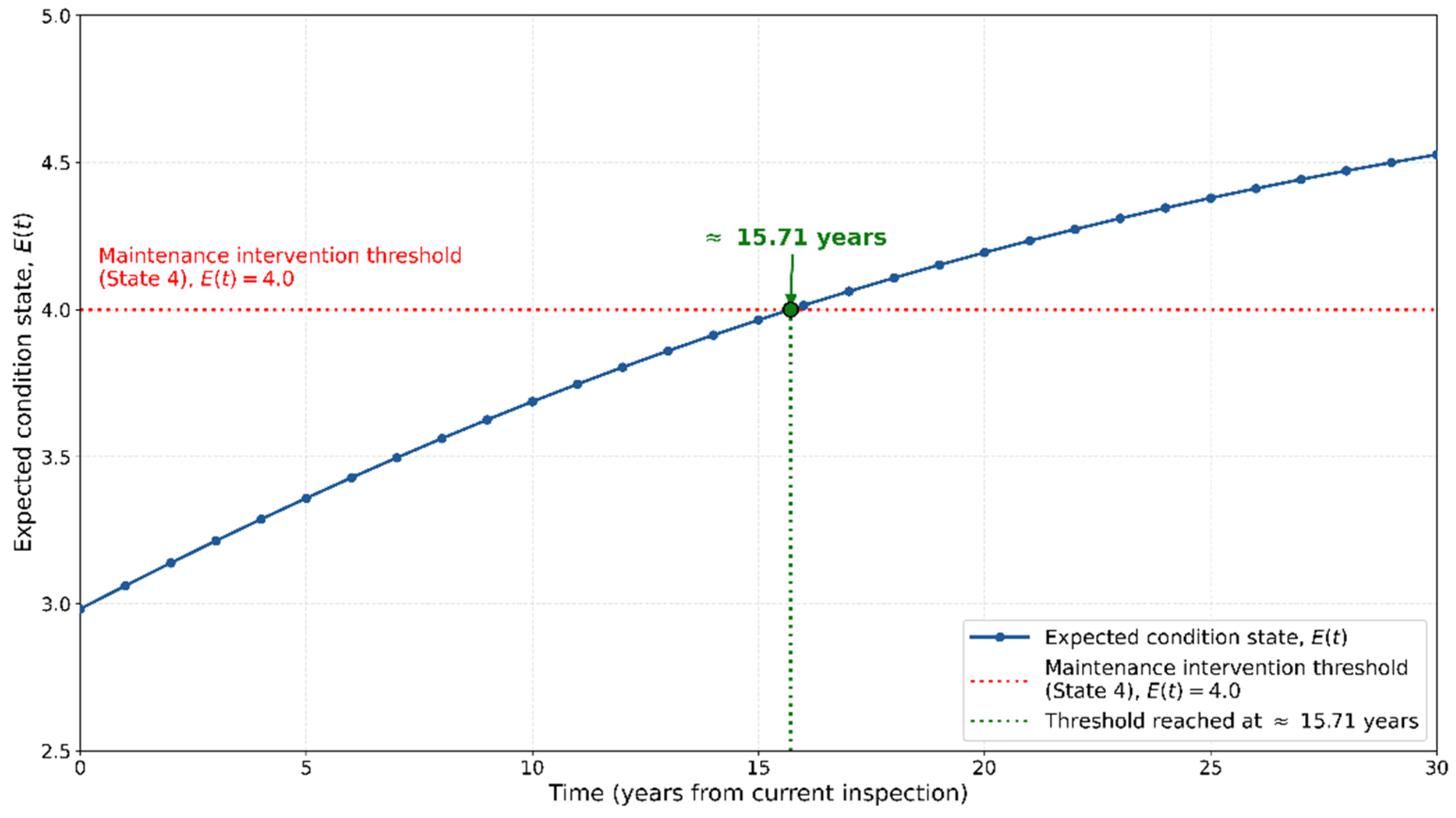
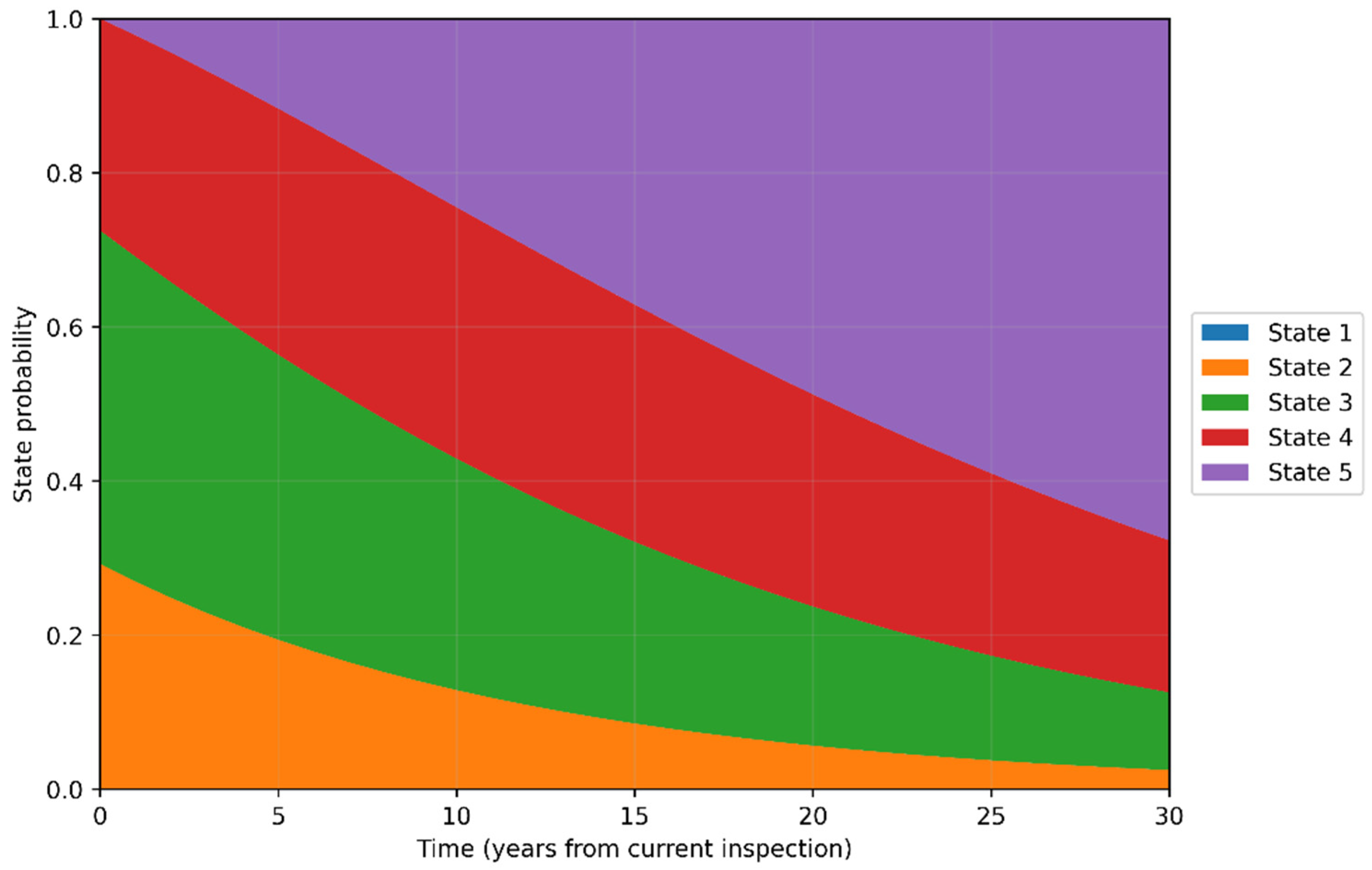
corresponding to an initial expected condition indicator of E(0) = 2.9825. Application of the bridge-specific transition probability matrix calibrated in Section 3.3 produced the predicted evolution of the expected bridge condition and the corresponding condition-state probability distribution under the do-nothing scenario, as presented in Figure 6 and Figure 7.

The expected condition indicator increases progressively from 2.9825 at the current inspection to 3.6871 after 10 years, 3.9647 after 15 years, and 4.0143 after 16 years. Interpolation between Years 15 and 16 indicates that the maintenance intervention threshold, defined by E(t) = 4.0, is reached after approximately 15.71 years. Because the Markov model operates at annual decision intervals, Year 16 represents the first discrete prediction at which the expected bridge condition exceeds the State 4 intervention threshold. This horizon should be interpreted as a planning benchmark under the do-nothing scenario rather than as a deterministic failure time.

The accompanying probability evolution demonstrates the progressive redistribution of the assessed bridge elements toward the poorer condition states. At the current inspection, the distribution is concentrated in States 2–4, with no assigned probability in State 5. Under continued do-nothing deterioration, the probability associated with State 5 increases to approximately 0.245 after 10 years, 0.371 after 15 years, and 0.395 after 16 years. Over the same period, the combined probability associated with States 4 and 5 increases from 0.275 at the current inspection to approximately 0.571 at Year 10 and 0.698 at Year 16. These results indicate a progressive concentration of the condition distribution in severe deterioration states when intervention is deferred.

The predicted intervention horizon is governed by the evolution of the bridge-level expected condition indicator and should not be interpreted as the time at which every bridge element simultaneously reaches State 4 or State 5. Rather, it represents the point at which the importance-weighted condition distribution yields an expected condition corresponding to the adopted State 4 maintenance intervention threshold. This distinction is important because individual elements already classified as State 4, particularly the pier columns, pier cap beams, and drainage system, require maintenance attention based on their current observed condition even though the bridge-level expected condition remains within State 3.

The recalibrated deterioration trajectory therefore provides a bridge-specific planning baseline for evaluating the consequences of continued inaction. The condition-rating-based RSL assessment presented in Section 4.4 is analytically independent of the Markov calibration and is subsequently compared with this Markov-derived intervention horizon at the level of predicted time scales. Agreement or divergence between the two estimates is interpreted as a cross-model consistency assessment rather than as formal validation of one model by the other.

4.4. Condition-Rating-Based Assessment and Remaining Service Life

The condition ratings obtained using the independent seven-point assessment method are summarized in

Table 6. Summary of condition ratings obtained using the condition-rating-based assessment method.

Component	Condition Rating (CR)
Main structural elements	4.83
Ground/soil-retaining elements	5.11
Service elements	5.63
Overall bridge	5.10
Pier columns (critical element)	3.67

Note: Bold text indicates the critical governing element and its condition rating.

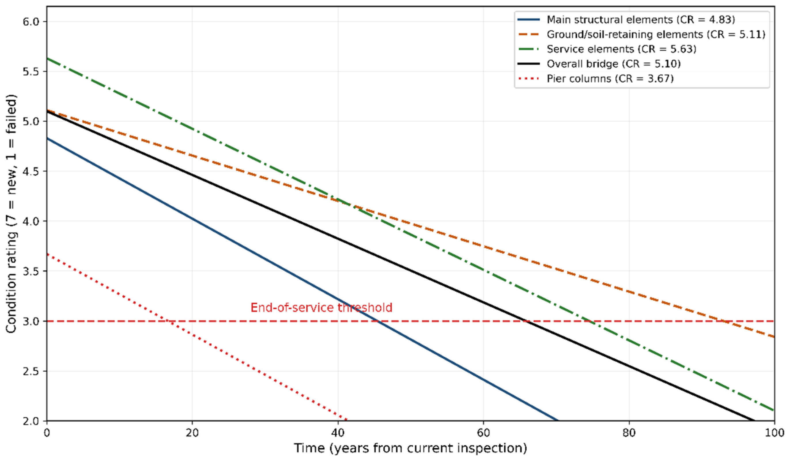
, while the complete element-level ratings and averaging calculations are documented in Appendix A (Table A2). The main structural elements achieved the lowest group rating (CR = 4.83), primarily because the pier columns were rated at only CR = 3.67, placing them close to the end-of-service threshold (CR = 3). In comparison, the ground/soil-retaining and service element groups achieved ratings of 5.11 and 5.63, respectively, resulting in a weighted overall bridge rating of CR = 5.10. These results indicate that, although the bridge remains in an acceptable overall condition, deterioration is concentrated in the most structurally critical load-carrying components.

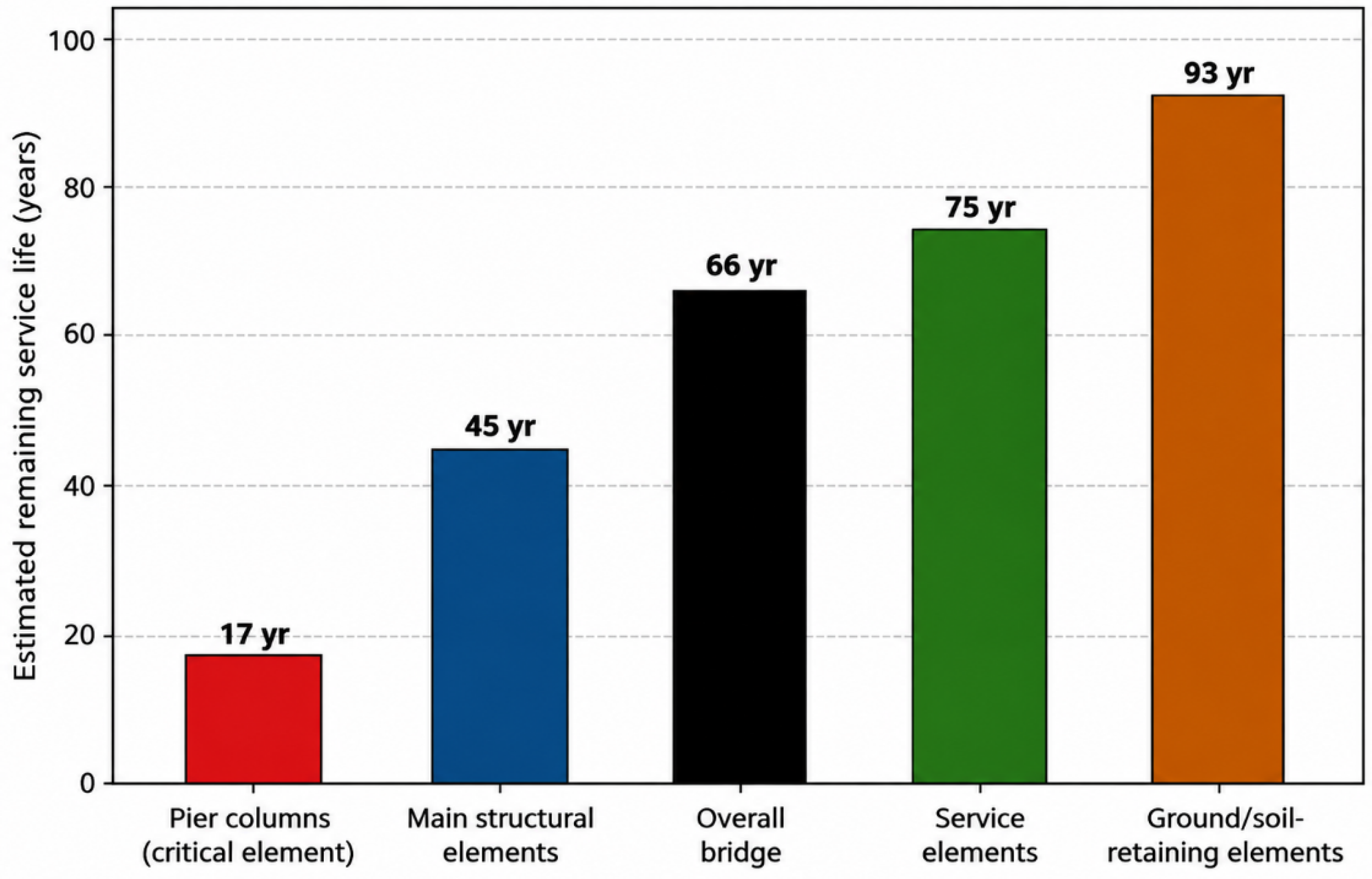
Application of the calibrated deterioration rates described in Section 3.4 converted the condition ratings into the linear deterioration trajectories shown in Figure 8 and the RSL estimates presented in Figure 9 and

Table 7. Remaining service life estimates obtained using the condition-rating-based assessment method.

Component	Rating CR	Rate DR (1/yr)	RSL (Years)
Main structural elements	4.83	0.0403	45
Ground/soil-retaining elements	5.11	0.0227	93
Service elements	5.63	0.0353	75
Overall bridge	5.10	0.0319	66
Pier columns (critical element)	3.67	0.0403	≈17

Note: Bold text indicates the critical governing element and its condition rating, deterioration rate, and remaining service life.

. In Figure 8, the horizontal threshold (CR = 3) denotes the end of economic service life. In addition, as shown in Figure 8, the effective service life of the bridge is governed by the critical pier columns rather than by the overall bridge condition.

The RSL values were calculated using Equation (7). The estimated RSL is 66 years for the overall bridge, 93 years for the ground/soil-retaining elements, 75 years for the service elements, and 45 years for the main structural elements. In contrast, the pier columns retain an estimated service life of only 17 years when evaluated individually using the deterioration rate of the main structural group. Because failure of the pier columns would directly compromise the structural stability of the bridge, the governing service life is controlled by this critical component rather than by the weighted average bridge condition.

The condition-rating-based assessment provides a complementary engineering perspective by explicitly identifying the structural components that govern the effective service life of the bridge. The substantial difference between the overall bridge RSL (66 years) and the pier-column RSL (17 years) demonstrates that maintenance priorities should be governed by the deterioration of critical load-carrying elements rather than by global bridge condition indicators alone. This component-oriented assessment establishes the basis for the comparative evaluation of the deterministic and stochastic deterioration approaches presented in the following section.

4.5. Comparison of Markov- and Condition Rating-Based Remaining Service Life Prediction

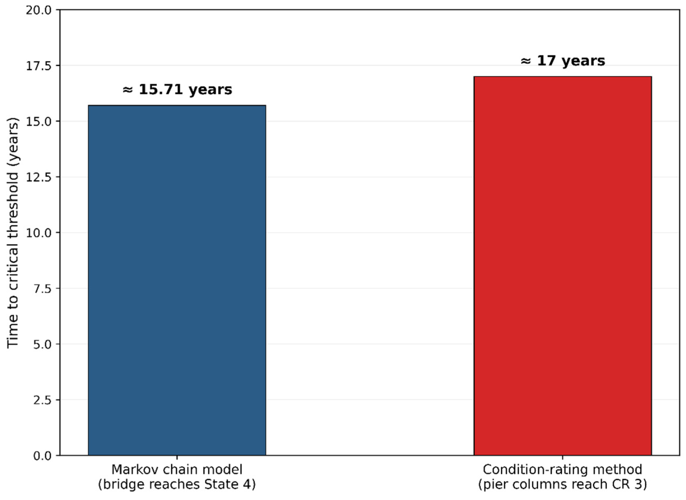
The intervention horizons predicted by the two independent deterioration assessment approaches are compared in Figure 10. The Markov deterioration model indicates that the bridge reaches the critical maintenance threshold (State 4) after approximately 15.71 years, with Year 16 representing the first discrete annual prediction exceeding the threshold, whereas the condition-rating-based assessment predicts that the governing pier columns reach the end-of-service threshold (CR = 3) after approximately 17 years. Although the two approaches are based on fundamentally different analytical principles (a probabilistic state-transition process and a deterministic deterioration-rate model), they consistently identify the need for maintenance intervention within the same decision-making period. This agreement increases confidence in the predicted intervention horizon under limited-data conditions. Importantly, this agreement was not imposed through the calibration procedure because the condition-rating-based RSL assessment was not used as a calibration target or constraint in the Markov model. The two indicators quantify different phenomena: the condition-rating-based estimate concerns the time at which the governing pier columns reach the seven-point end-of-service threshold, whereas the Markov prediction concerns the time at which the importance-weighted overall bridge condition reaches State 4. Because the two measures are defined on different scales, aggregated over different structural scopes, and driven by different deterioration formulations (a deterministic fleet-average rate versus a bridge-specific stochastic process), their close correspondence provides an independent cross-model consistency check rather than a calibration-imposed agreement. The close agreement between the two estimates, despite these methodological differences, indicates that the deterioration information extracted from the single inspection is internally consistent.

The two approaches also provide complementary decision-support information. The Markov model describes the temporal evolution of deterioration and the increasing probability of transition to poorer condition states (Figure 7), thereby supporting network-level deterioration forecasting and risk-informed maintenance planning. In contrast, the condition-rating-based approach estimates the remaining service life of individual bridge components (Figure 9), enabling maintenance prioritization according to the deterioration of critical structural elements. For bridges lacking historical inspection records, the combined application of both approaches following a single detailed inspection offers a practical and cost-effective framework by integrating stochastic deterioration prediction with component-level engineering assessment.

The predicted intervention horizons assume that current environmental exposure and deterioration mechanisms remain unchanged. However, deterioration may progress more rapidly because of potential scour beneath the western abutment and around the mid-river pier platforms, where underwater regions could not be directly inspected, as well as extreme hydraulic or ice-loading events acting on the already deteriorated pier columns. Conversely, timely rehabilitation of the drainage and expansion-joint systems would be expected to reduce moisture-related deterioration and delay the progression toward critical condition states. Since destructive testing was administratively prohibited during the present study, future investigations should complement the proposed assessment framework with code-compliant structural performance (load-rating) evaluations to further improve the reliability of long-term deterioration predictions.

4.6. MDP-Based Maintenance Optimization Results

The maintenance optimization was performed using the computational workflow presented in Figure 3. The Markov Decision Process (MDP) was solved over a 50-year planning horizon by backward dynamic programming using the bridge-specific deterioration model, action-dependent transition probability matrices, maintenance-effect models, normalized intervention costs, and the initial bridge condition distribution obtained from the inspection results. The initial condition vector, Q(0) = [0, 0.2925, 0.4325, 0.2750, 0], corresponds to an expected bridge condition of E(0) = 2.98, consistent with the weighted bridge condition index obtained in Section 4.2.

At the beginning of the planning horizon, the optimal maintenance policy follows a clear condition-dependent strategy (

Table 8. Initial optimal maintenance actions by bridge condition state.

Condition State	Condition Description	Optimal Action	Recommended Intervention Level
1	Very good	A0	Do nothing and continue routine inspection
2	Good	A1	Preventive maintenance
3	Fair	A2	Corrective repair
4	Poor	A3	Major rehabilitation
5	Very poor/critical	A3	Major rehabilitation or replacement-level intervention

): routine monitoring is selected for State 1, preventive maintenance for State 2, corrective repair for State 3, and major rehabilitation for States 4 and 5. This initial policy remains unchanged over most of the 50-year horizon. Because the optimization is finite-horizon, however, the optimal action becomes time-dependent near the terminal years; therefore, Table 8 should be interpreted as the initial and principal state-dependent intervention rule rather than as a stationary policy applying identically throughout the entire planning horizon. This hierarchy demonstrates that delaying intervention until advanced deterioration is reached is not economically optimal under the adopted life-cycle cost structure. Preventive maintenance is preferred in State 2 because relatively low intervention costs reduce future deterioration, whereas corrective repair becomes more beneficial in State 3 and major rehabilitation is preferred for States 4 and 5.

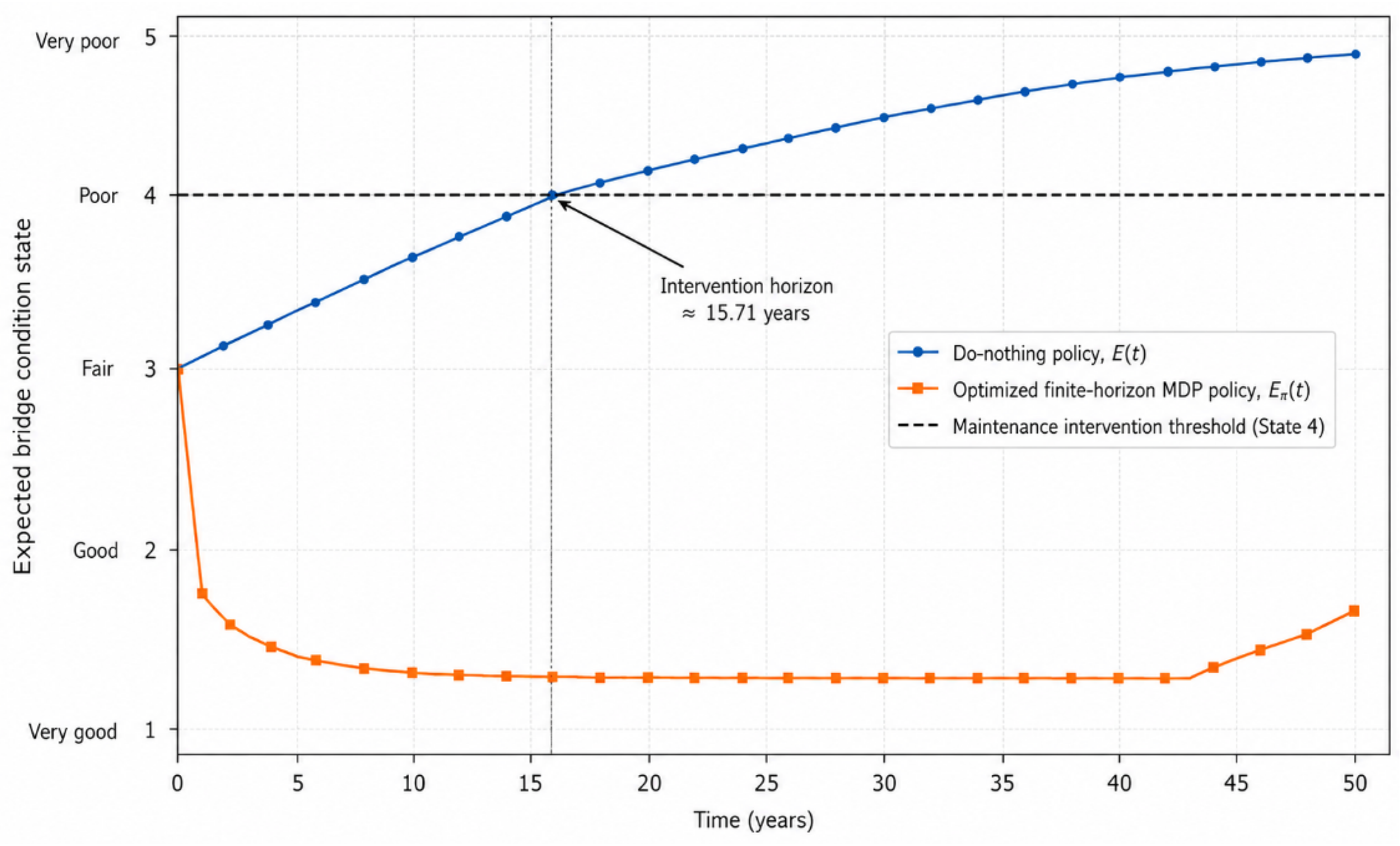
Application of the optimized policy substantially changes the long-term deterioration trajectory compared with the do-nothing scenario. Under the do-nothing policy, the expected bridge condition increases from 2.98 to 4.014 at Year 16, consistent with the Markov deterioration prediction presented in Section 4.3 and with the interpolated State-4 intervention threshold of approximately 15.71 years. In contrast, implementation of the optimized policy reduces the expected condition to approximately 1.75 after the first decision cycle because the existing State-3 and State-4 portions receive corrective repair and major rehabilitation, respectively. The expected condition subsequently remains within the State 1–State 2 range over most of the planning horizon, as preventive, corrective, and rehabilitation actions limit the accumulation of probability in the poorer states. The corresponding deterioration trajectories are presented in Figure 11 and summarized in

Table 9. Expected bridge condition under the do-nothing and optimized finite-horizon MDP policies.

Year	Do-Nothing Policy, E(t)	Optimized Policy, Eπ(t)
0	2.98	2.98
1	3.06	1.75
3	3.21	1.52
5	3.36	1.42
10	3.69	1.33
16	4.01	1.31
20	4.19	1.31
50	4.85	1.71

.

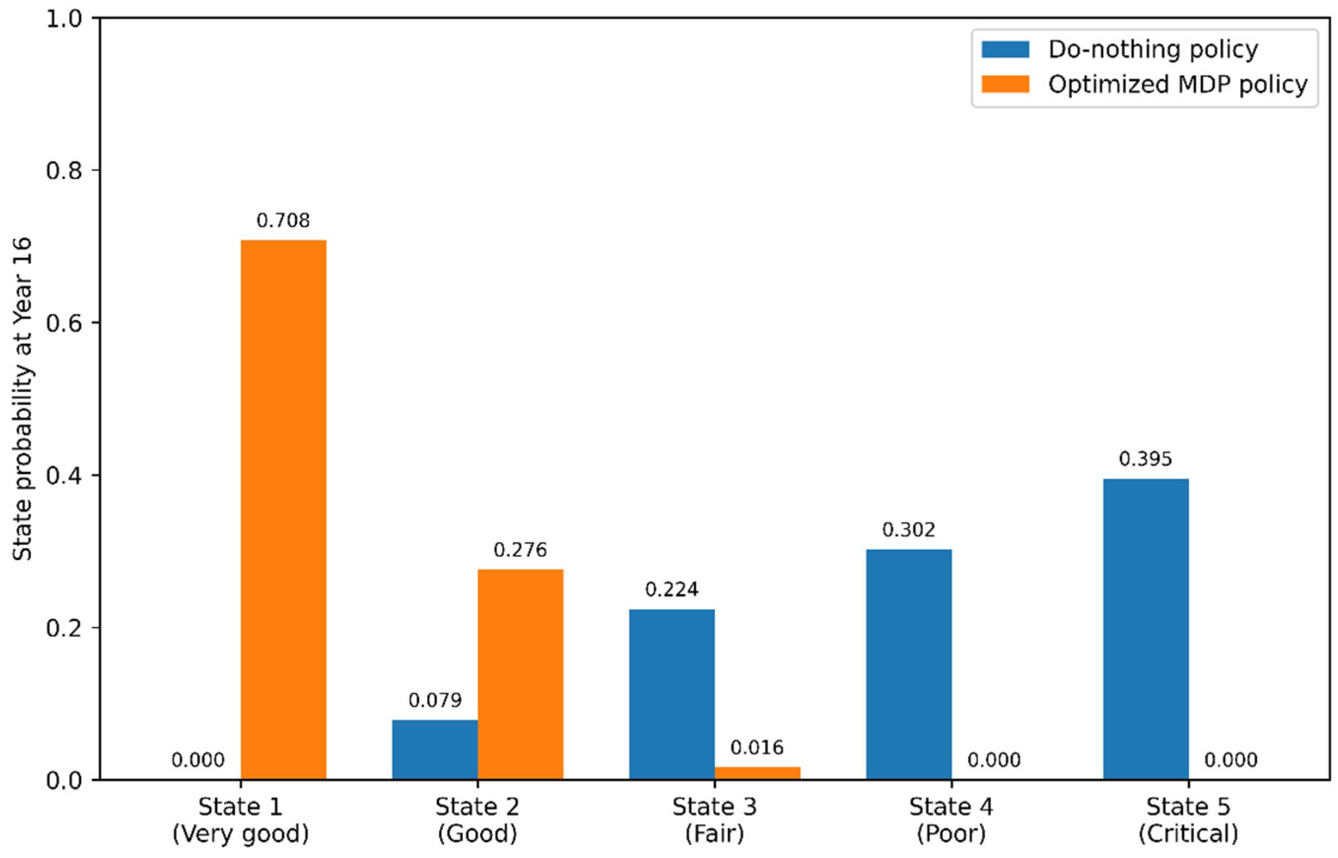
The optimized maintenance strategy also produces a fundamentally different condition-state distribution. At Year 16, the optimized finite-horizon MDP policy concentrates approximately 70.8% of the bridge condition probability in State 1 and 27.6% in State 2, with only 1.6% remaining in State 3 and no probability assigned to States 4 and 5. Under the do-nothing policy, however, approximately 69.8% of the bridge-weighted probability accumulates in States 4 and 5, including approximately 39.5% in State 5. Figure 12 and

Table 10. Condition-state probability distribution at Year 16.

Policy	State 1	State 2	State 3	State 4	State 5
Do nothing	0.000	0.079	0.224	0.302	0.395
Optimized finite-horizon MDP policy	0.708	0.276	0.016	0.000	0.000

demonstrate that the optimized finite-horizon policy redirects the condition distribution toward the better condition states and prevents the accumulation of probability in the poor and critical states.

The corresponding life-cycle cost analysis further highlights the effectiveness of the optimized policy. Using the normalized maintenance-cost structure and a 3% annual discount rate, the expected discounted 50-year cost decreases from 442.21 under the do-nothing strategy to 45.32 under the optimized finite-horizon MDP policy, corresponding to an approximately 89.75% reduction (

Table 11. Fifty-year life-cycle performance comparison.

Performance Measure	Do-Nothing Policy	Optimized Finite-Horizon MDP Policy
Expected discounted cost	442.21	45.32
Relative cost reduction	—	89.75%
Expected condition at Year 16	4.01	1.31
Probability of State 5 at Year 16	0.395	0.000
Probability of States 4–5 at year 16	0.698	0.000
Critical threshold reached	≈15.71 years	Not reached within the 50-year horizon
Dominant condition at Year 16	States 4–5	States 1–2

). Because normalized costs were adopted, this value should be interpreted as an indicator of relative economic efficiency rather than a project-specific monetary saving. Nevertheless, the comparison clearly demonstrates that early preventive and corrective interventions substantially reduce long-term deterioration penalties and produce more economical maintenance strategies than deferring intervention until severe deterioration develops.

Overall, the optimization results demonstrate that integrating inspection-based condition assessment, stochastic deterioration modelling, and optimization-based decision-making enables maintenance actions to be scheduled according to their expected long-term structural and economic consequences rather than fixed deterioration thresholds alone. The resulting optimal policy therefore provides the quantitative basis for translating bridge-level maintenance decisions into element-level intervention strategies, as presented in the following section.

4.6.1. Initial Optimized Intervention for the Case-Study Bridge

Application of the initial optimized maintenance policy to the case-study bridge results in a differentiated intervention program because the current bridge condition includes elements classified in States 2, 3, and 4. Accordingly, preventive maintenance is assigned to the State 2 components, corrective repair to the State 3 components, and major rehabilitation to the State 4 components. The resulting translation of the optimized policy into element-level maintenance actions is summarized in

Table 12. Translation of the initial optimized maintenance policy into element-level intervention measures.

Current State	Bridge Elements	MDP Action	Principal Recommended Measures
2	Steel girders, cross-bracings, foundations/platform, curbs, sidewalks, railings and barriers	Preventive maintenance	Cleaning, corrosion treatment, protective coating, minor sealing and routine inspection
3	Deck slab, bearings, abutments, approach fill/slab, slope protection, wearing surface and expansion joints	Corrective repair	Concrete repair, reinforcement protection, crack treatment, joint repair, surfacing and stabilization works
4	Pier columns, pier cap beams and drainage system	Major rehabilitation	Structural concrete rehabilitation, reinforcement repair or strengthening, drainage reconstruction and moisture-control measures

.

The State 4 pier columns, pier cap beams, and drainage system constitute the highest maintenance priority because field inspections identified advanced concrete deterioration, reinforcement exposure, corrosion, leakage, and ineffective surface-water drainage. The optimized MDP policy therefore directly reflects the deterioration mechanisms observed during the bridge inspection, demonstrating the consistency between the optimization results and the engineering assessment.

Although the western abutment was assigned to State 3, the suspected scour beneath the abutment requires separate consideration because the potential consequences of foundation instability are not fully represented by the bridge-level condition-state cost model. Therefore, underwater inspection together with detailed hydraulic and geotechnical investigations should be undertaken as an immediate risk-control measure independently of the optimized maintenance policy.

4.6.2. Comparison with Conventional Threshold-Based Maintenance

Conventional threshold-based maintenance typically postpones intervention until bridge components reach a predefined deterioration state, commonly State 4, thereby reducing short-term expenditure but allowing deterioration to progress through intermediate condition states. As deterioration accumulates, the probability of requiring major rehabilitation increases together with the associated life-cycle costs. In contrast, the optimized MDP policy recommends preventive maintenance in State 2 and corrective repair in State 3 whenever the expected long-term reduction in deterioration and rehabilitation costs exceeds the immediate intervention cost. Consequently, maintenance decisions are based on anticipated future system performance rather than solely on the current condition state.

For the case-study bridge, this difference is particularly evident for the drainage system and expansion joints. Although these service components are not the primary load-carrying elements, deficiencies in drainage accelerate moisture ingress, reinforcement corrosion, concrete deterioration, and subsequent degradation of adjacent structural members. By explicitly accounting for future deterioration pathways and maintenance effects, the optimized policy prioritizes timely intervention for these components before severe structural damage develops, demonstrating the practical engineering value of the proposed decision framework.

To provide a quantitative benchmark beyond the do-nothing comparison, the optimized finite-horizon MDP policy was also evaluated against two conventional reactive strategies under identical transition, cost, discount-rate, and planning-horizon assumptions. A fixed-threshold policy applying major rehabilitation upon reaching States 4–5 produced an expected discounted 50-year cost of 79.97 normalized units, while a reactive policy applying corrective repair in State 4 and major rehabilitation in State 5 produced a cost of 122.47 units. The corresponding optimized MDP cost was 45.32 units, compared with 442.21 units under the do-nothing strategy. Thus, although both threshold-based strategies substantially improved performance relative to no intervention, the optimized policy achieved the lowest expected discounted cost by allowing preventive and corrective actions to be selected before severe deterioration became dominant. These values are scenario-relative outcomes under the adopted normalized cost assumptions and should not be interpreted as project-specific monetary savings.

Table 13. Comparison between conventional threshold-based maintenance and the proposed inspection-driven Markov–RSL–MDP framework.

Criterion	Conventional Threshold-Based Maintenance	Proposed Inspection-Driven Markov–RSL–MDP Framework	Evidence from the Present Study
Decision principle	Fixed intervention threshold	Dynamic optimization based on the Bellman optimality principle	State-dependent optimal maintenance policy obtained by backward dynamic programming
Maintenance timing	Reactive	Proactive	Preventive and corrective actions initiated before severe deterioration becomes dominant
Future deterioration	Not explicitly considered	Explicitly predicted using the bridge-specific Markov deterioration model	Critical intervention threshold predicted after approximately 15.71 years
Maintenance effects	Generally assumed	Explicitly represented through action-dependent transition models	Preventive, corrective, and rehabilitation actions evaluated independently
Remaining service life	Usually evaluated separately or omitted	Independently assessed and used as a complementary decision-support benchmark	Estimated RSL: 66 years (overall bridge), 45 years (main structural system), and approximately 17 years (pier columns)
Life-cycle cost	Not optimized	Explicitly minimized	50-year discounted normalized cost: 45.32 for the optimized MDP, compared with 79.97 for fixed-threshold rehabilitation, 122.47 for reactive repair/rehabilitation, and 442.21 for do nothing
Adaptability	Limited	High	Transition probabilities and maintenance policies can be updated following future inspections

summarizes the principal differences between conventional threshold-based maintenance and the proposed inspection-driven Markov–RSL–MDP framework together with the corresponding evidence obtained from the present case study.

The comparison demonstrates that the principal advantage of the proposed framework is not the replacement of conventional engineering judgment, but its quantitative support. By integrating inspection results, bridge-specific deterioration modelling, remaining service life prediction, maintenance-effect modelling, and life-cycle cost optimization within a unified decision framework, maintenance actions can be prioritized according to their expected long-term structural and economic consequences. This provides a systematic transition from fixed threshold-based maintenance toward condition-dependent, optimization-based intervention planning, particularly for bridges where historical inspection data are limited.

4.7. Sensitivity Analysis and Robustness Assessment

To evaluate the robustness of the proposed inspection-driven Markov–RSL–MDP framework, a quantitative sensitivity analysis was performed by varying the principal economic, maintenance-effect, deterioration, and transition-model assumptions. The examined scenarios included variations in maintenance action costs (±20%), state penalties (±20%), maintenance-effect probabilities (±20%), discount rate (1–5%), planning horizon (25–75 years), do-nothing deterioration intensity (0.8–1.2 times the baseline level), and the structural shape of the transition probability matrix (TPM). For each scenario, the finite-horizon MDP was re-solved and the resulting maintenance policy, predicted bridge condition, and life-cycle cost were compared with the baseline solution. The quantitative results are summarized in

Table 14. Quantitative sensitivity and robustness assessment of the optimized finite-horizon MDP policy.

Parameter Group	Scenario	Optimized Discounted Cost	Cost Reduction Relative to Do Nothing (%)	Expected Condition at Year 16	State 1 Probability at Year 16	Initial Optimal Policy	Policy Agreement, Years 0–12 (%)
Baseline	Baseline	45.32	89.75	1.308	0.708	DN–PM–CR–MR–MR	100
Maintenance action cost	−20%	39.47	91.07	1.308	0.708	DN–PM–CR–MR–MR	100
Maintenance action cost	+20%	51.14	88.43	1.308	0.708	DN–PM–CR–MR–MR	100
State penalties	−20%	42.07	88.11	1.308	0.708	DN–PM–CR–MR–MR	100
State penalties	+20%	48.54	90.85	1.308	0.708	DN–PM–CR–MR–MR	100
Maintenance effectiveness	−20%	54.09	87.77	1.369	0.655	DN–PM–CR–MR–MR	100
Maintenance effectiveness	+20%	40.62	90.81	1.265	0.747	DN–PM–CR–MR–MR	100
Discount rate	1%	58.44	92.12	1.308	0.708	DN–PM–CR–MR–MR	100
Discount rate	5%	37.80	86.76	1.308	0.708	DN–PM–CR–MR–MR	100
Planning horizon	25 years	36.31	84.61	1.308	0.708	DN–PM–CR–MR–MR	100
Planning horizon	75 years	49.63	91.08	1.308	0.708	DN–PM–CR–MR–MR	100
Do-nothing deterioration intensity	px0.8	42.20	89.41	1.264	0.750	DN–PM–CR–MR–MR	100
Do-nothing deterioration intensity	px1.2	48.16	89.94	1.348	0.670	DN–PM–CR–MR–MR	100
TPM structural shape	State-dependent mild	40.62	91.32	1.240	0.773	DN–PM–CR–MR–MR	100
TPM structural shape	State-dependent strong	37.97	92.05	1.202	0.809	DN–PM–CR–MR–MR	100

Note: DN = do nothing/monitoring; PM = preventive maintenance; CR = corrective repair; MR = major rehabilitation. The probabilities of States 4 and 5 at Year 16 were effectively zero in all examined optimized scenarios. Cost-reduction percentages were calculated relative to the corresponding do-nothing solution under the same discount rate and planning horizon. The sensitivity analysis represents an engineering scenario-based robustness assessment rather than a statistical uncertainty or confidence analysis.

.

The analysis indicates that the optimized maintenance strategy remained stable throughout the examined parameter ranges, with 100% agreement in the initial optimal policy over Years 0–12 across all sensitivity scenarios. Variations in maintenance action costs, state penalties, discount rate, and planning horizon primarily affected the economic outcomes, whereas changes in maintenance effectiveness, do-nothing deterioration intensity, and TPM structural shape produced moderate variations in the predicted post-intervention condition. Despite these variations, the recommended state-dependent intervention sequence remained unchanged. These findings demonstrate that the proposed framework is robust to reasonable perturbations in the principal economic, deterioration, maintenance-effect, and transition-model assumptions considered in the analysis.

To provide a more informative assessment of policy stability than the initial policy mapping alone, the baseline time-dependent switching boundaries were also examined. State 1 retained do nothing/monitoring throughout decision Years 0–49, while State 5 retained major rehabilitation throughout the same period. For State 2, preventive maintenance was optimal in Years 0–42 and changed to do nothing/monitoring in Years 43–49. For State 3, corrective repair was optimal in Years 0–47 and changed to do nothing/monitoring in Years 48–49. For State 4, major rehabilitation was optimal in Years 0–47 and changed to corrective repair in Years 48–49. These late-horizon switches reflect the decreasing opportunity to recover the future benefits of intervention as the terminal epoch approaches. Across the examined sensitivity scenarios, policy agreement with the baseline was 100% over Years 0–12, whereas full common-horizon agreement ranged from 91.2% to 100.0%, with the differences concentrated near the terminal years. The reported 100% early-policy agreement should therefore not be interpreted as complete policy invariance over the entire finite horizon.

To address the epistemic uncertainty associated with the engineering-calibrated deterioration model itself (Section 3.3), the robustness assessment was further extended beyond economic and maintenance parameters to the deterioration and transition-model assumptions. The do-nothing deterioration intensity was varied to 0.8 and 1.2 times its baseline level, and additional state-dependent TPM shapes were examined as structural stress tests of the calibrated transition model. As shown in Table 14, these perturbations changed the predicted Year-16 condition and State-1 probability but did not alter the initial optimal condition–action mapping, for which policy agreement over Years 0–12 remained 100% in every examined scenario. This stability is particularly relevant because the baseline do-nothing trajectory reaches the State-4 intervention threshold at approximately 15.71 years, whereas the optimized policy is state-dependent rather than triggered by a fixed calendar year. The sensitivity results therefore indicate that reasonable perturbations of the deterioration intensity and TPM structure affect the predicted condition trajectory without changing the principal early- and medium-term maintenance strategy.

Overall, the sensitivity analysis indicates that the principal maintenance recommendations remain stable under the examined variations in economic, maintenance, deterioration, and transition-model assumptions. Although the numerical values of the predicted costs and condition indicators vary among scenarios, the optimized decision strategy remains consistent, supporting its applicability to practical bridge management under limited historical deterioration information.

4.8. Implications for Bridge Management, Limitations, and Future Research

Many existing bridges, particularly those managed by local authorities, lack the long-term inspection records required by conventional Bridge Management Systems. The proposed framework addresses this limitation by converting the results of an initial comprehensive inspection directly into optimized maintenance decisions. By combining stochastic deterioration prediction, an independent Remaining Service Life assessment, and MDP-based optimization, it extends condition assessment into actionable intervention planning. For the investigated bridge, the optimized policy prioritizes the drainage system, expansion joints, pier columns, and cap beams, indicating that maintenance should address not only severely deteriorated elements but also components that accelerate system-level deterioration.

The optimization results should nevertheless be interpreted as decision-support recommendations rather than automatic maintenance instructions. Their implementation must also consider structural safety, hydraulic and scour conditions, constructability, traffic management, available budgets, and agency-specific constraints. In addition, the transition probabilities were derived from engineering judgement supported by published deterioration characteristics because systematic inspection records were unavailable. The maintenance-effect matrices and normalized costs likewise represent transparent engineering assumptions used for decision-support demonstration rather than statistically calibrated or project-specific values. The present screening-level formulation also assigns one governing condition state to each assessed element category and applies a common condition-state transition structure across heterogeneous component types. Quantitative deterioration-extent fractions within individual categories and element-type-specific deterioration or intervention-response matrices could not be established from the available inspection records. Consequently, the resulting bridge-level distribution and element-level action assignments should be interpreted as importance-weighted category representations rather than as a unit-by-unit physical-state model of the bridge. A further limitation is that visual inspection constituted the sole condition-information source; non-destructive testing techniques such as ultrasonic pulse velocity, rebound hammer, half-cell corrosion potential mapping, and ground-penetrating radar were beyond the administrative scope of the present campaign and would provide valuable quantitative refinement of the element condition states in future applications. Deterioration was assumed stationary, while time-dependent mechanisms, environmental and traffic variability, extreme events, user costs, sustainability, resilience, and network-level budget allocation were outside the scope of the present single-bridge application.

These limitations provide clear directions for further development. The model components may be progressively recalibrated using periodic inspection data through frequency-based estimation, Bayesian updating, maximum-likelihood methods, hidden Markov models, and machine learning-assisted estimation. Integration with structural health monitoring, digital twin, and UAV-based inspection technologies could further improve prediction and updating capabilities [18,19,21], while inspection-data-driven machine learning models offer complementary means of estimating remaining service life directly from condition records [20]. Reinforcement learning, approximate dynamic programming, and POMDP formulations also offer promising extensions for asset- and network-level maintenance under uncertainty and partial observability [36,37,38,40,42,48,49], while multi-objective formulations incorporating sustainability, resilience, and user costs provide a natural extension of the present cost-based objective [41,50]. In this context, the purpose of the single-bridge application should be stated explicitly: it is methodological demonstration rather than statistical generalization. The case study establishes that the complete inspection-to-decision chain can be executed, audited, and stress-tested on a real structure; it does not claim that its numerical outcomes generalize to other bridges. Because the demonstration is limited to a single case-study bridge, the transferability of the framework has not yet been established empirically. Systematic application to multiple bridges of different structural types, ages, and exposure environments (ideally including structures for which longitudinal inspection records exist, so that the engineering-calibrated predictions can be benchmarked directly against statistically estimated deterioration models) constitutes the most direct route to such validation. It should nevertheless be noted that the computational architecture of the framework is bridge-agnostic. Application to a different structure requires bridge-specific inspection and condition-state data, element and subsystem weighting information, deterioration-calibration inputs, feasible maintenance actions and their transition effects, intervention costs, and the relevant economic and planning parameters; these inputs should be adapted to the structural system, deterioration mechanisms, exposure conditions, and agency-specific maintenance practice rather than transferred directly from the present case study.

With respect to external validation, an explicit staged protocol is proposed. In the short term, the calibrated model produces falsifiable predictions for the investigated bridge itself: under the do-nothing scenario, the expected condition is predicted to increase from 2.98 to approximately 3.06 after one year and 3.21 after three years (Table 9). The first scheduled follow-up inspection will therefore provide a direct out-of-sample test of the calibrated deterioration model, after which the transition probabilities can be re-estimated with the new observation included, for example through the Bayesian updating scheme outlined above. In the medium term, application of the framework to bridges for which longitudinal inspection records already exist would allow the engineering-calibrated predictions to be benchmarked directly against statistically estimated deterioration models, providing external validation at the methodological rather than the single-structure level.

5. Conclusions

This study presented an integrated framework that combines inspection-based condition assessment, a five-state Markov deterioration model, an independent condition-rating-based Remaining Service Life (RSL) assessment, and Markov Decision Process (MDP)-based maintenance optimization for existing highway bridges without historical inspection records. The principal findings and contributions are summarized as follows:

• Application of the framework to a 26-year-old composite highway bridge demonstrated that a rational, fully quantitative deterioration assessment can be achieved from a single comprehensive inspection. The weighted Bridge Condition Index (CI = 2.98) classified the bridge as moderately deteriorated, with the pier columns, cap beams, drainage system, and expansion joints identified as the governing components, and this classification was shown to be robust to ±20% variations in the weighting coefficients.
• The calibrated Markov model predicted attainment of the State-4 intervention threshold after approximately 15.71 years under the do-nothing strategy, while the independent condition-rating-based assessment estimated a remaining service life of approximately 17 years for the governing pier columns (66 years for the overall bridge). The close correspondence between these independent estimates, together with the sojourn-time and deterioration-rate plausibility checks, supports the engineering plausibility of the predicted intervention window under limited-data conditions.
• Integrating the finite-horizon MDP transformed deterioration prediction into an optimization-based decision-support process. The resulting state-dependent policy—routine inspection in State 1, preventive maintenance in State 2, corrective repair in State 3, and major rehabilitation in States 4 and 5—reduced the expected discounted 50-year life-cycle cost from 442.21 to 45.32 in normalized cost units, corresponding to an 89.75% reduction relative to the do-nothing strategy. At Year 16, the optimized trajectory maintained an expected condition of 1.31, compared with 4.01 under do nothing, while the probability of occupying States 4–5 was effectively zero under the optimized policy.
• The quantitative sensitivity analysis demonstrated that the optimized maintenance strategy remained stable across the examined variations in maintenance action costs, state penalties, maintenance effectiveness, discount rates, planning horizons, do-nothing deterioration intensity, and TPM structural shape. The initial optimal policy showed 100% agreement over Years 0–12 in all examined scenarios, although the predicted costs and post-intervention condition indicators varied. These results support the robustness of the principal state-dependent maintenance strategy to the engineering and economic perturbations considered in the analysis.
• The principal contribution of this study is the development of an inspection-driven computational framework that systematically integrates bridge inspection, stochastic deterioration prediction, independent RSL estimation, and optimization-based maintenance planning into a transparent and reproducible decision-support methodology. The framework provides a practical solution for bridge inventories with limited historical deterioration information, while its modular architecture enables progressive refinement as new inspection data become available, offering a practical pathway toward more data-driven Bridge Management Systems.