QueryFieldNet: A Query-Conditioned Surrogate Model for Multi-Beam Reflectarray Principal-Cut Gain Prediction

Abstract
1. Introduction
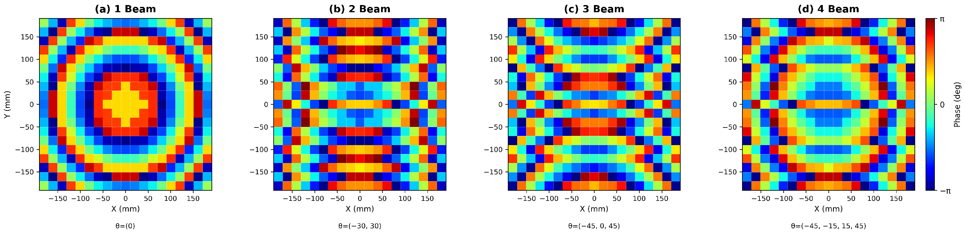
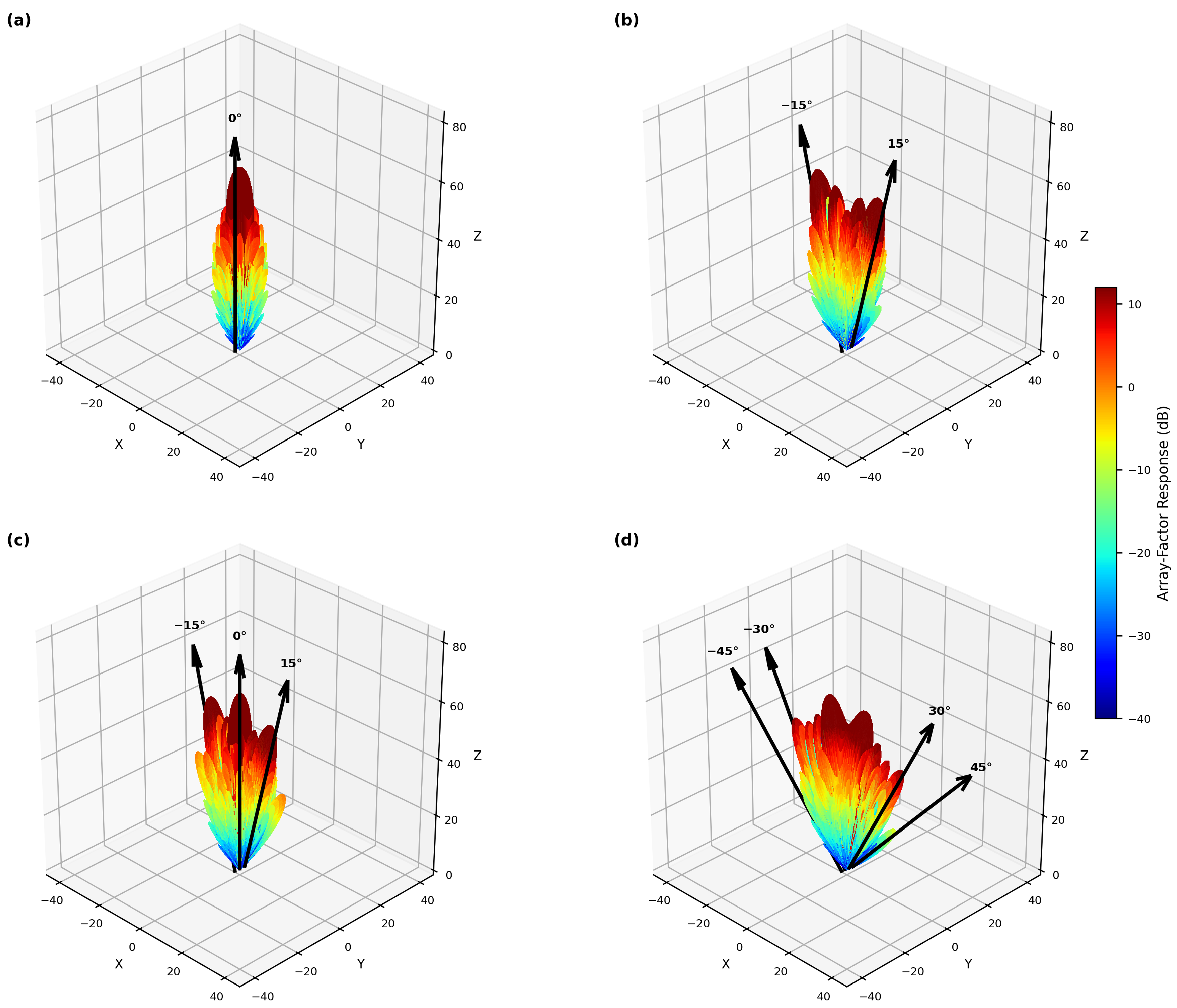
- A fixed--grid multi-beam reflectarray dataset is constructed for phase quantization levels from 1-bit to 5-bit. For each bit depth, 2000 phase maps and two orthogonal principal-cut wide-angle gain curves are generated.
- Multi-Beam HPBW RMSE, Multi-Beam Main-Lobe RMSE, and Beam-Peak RMSE are defined to address the limitation that conventional HPBW RMSE and Main-Lobe RMSE are primarily suited to single-beam evaluation.
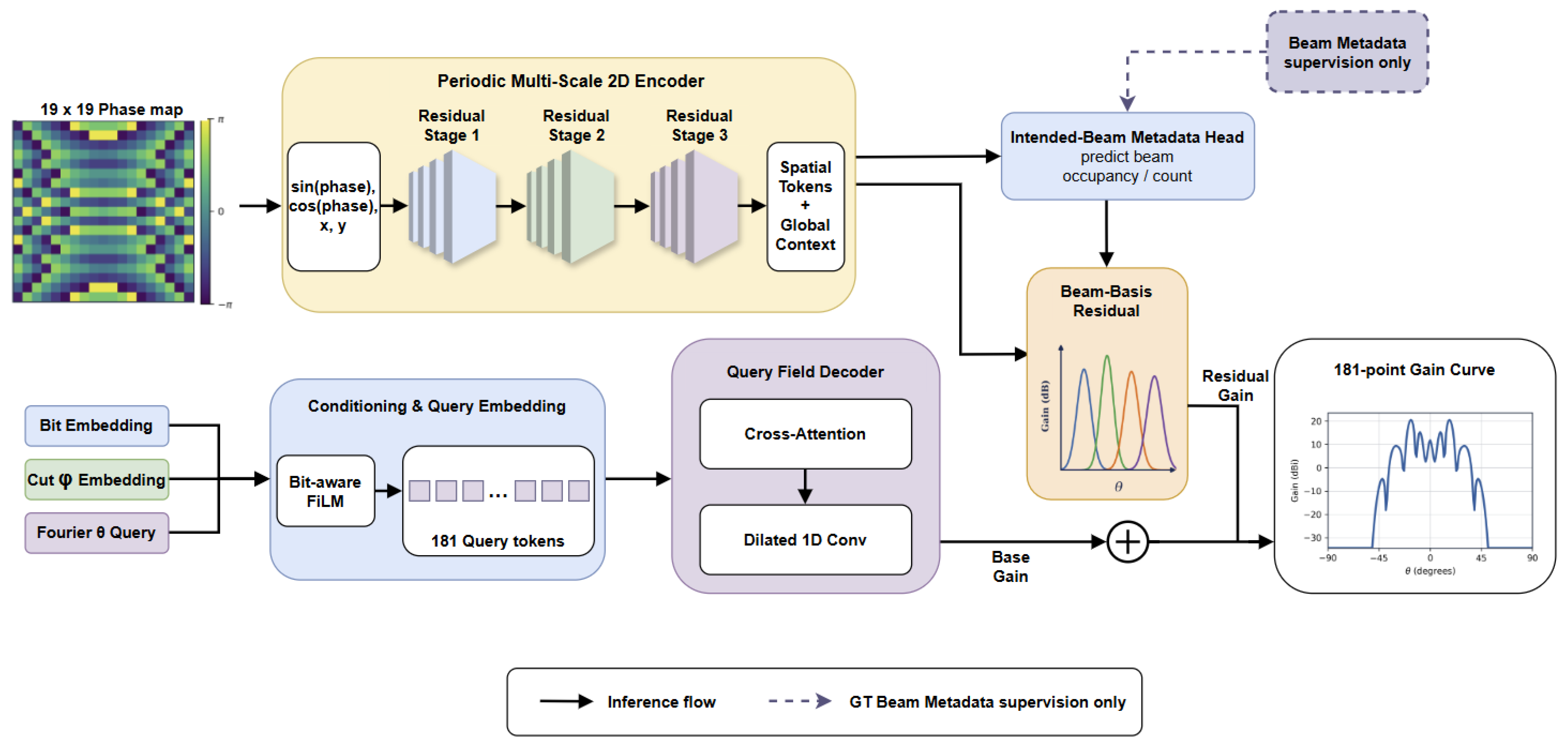
- QueryFieldNet is proposed to predict wide-angle gain fields by combining 2D phase maps and angular queries. The proposed model incorporates local multi-beam structures through an intended-beam metadata head and a beam-basis residual branch.
- QueryFieldNet is compared with adapted baselines reconstructed from published machine-learning and antenna surrogate modeling approaches for the phase-map-based 181-point gain-curve prediction setting. Detailed bit-depth, beam-count, and -position analyses are provided under fixed--grid multi-beam conditions.
2. Method
2.1. Problem Formulation
2.2. Multi-Beam Reflectarray Dataset Generation
2.3. Algorithmic Description of Dataset Generation
| Algorithm 1 Sample-Specific b-bit Phase-Level LUT Generation |
| Require: bit depth b, target sample count N, LUT template Ensure: N sample-specific b-bit phase-level lookup tables
|
| Algorithm 2 Balanced Fixed-Grid Multi-Beam Target Sampling |
| Require: theta grid , beam-count range Ensure: multi-beam target list B
|
| Algorithm 3 Multi-Beam Phase Map and Gain Curve Generation |
| Require: bit depth b, phase-level LUT, beam target list B, MRA array-factor-level reflectarray simulator Ensure: phase maps, principal-cut gain curves, and sample metadata Fixed parameters: frequency = 8 GHz; square reflectarray phase-map grid; cell pitch = 20.1 mm aperture-mask side length mm; all cell centers retained feed position mm; phase-map size output to ; output cut
|
2.4. HPBW, Main-Lobe, and Proposed Multi-Beam Metrics
2.4.1. Multi-Beam HPBW RMSE
2.4.2. Multi-Beam Main-Lobe RMSE
2.4.3. Beam-Peak RMSE
2.5. QueryFieldNet Architecture
2.5.1. Periodic Phase Input Encoding
2.5.2. Periodic Multi-Scale 2D Encoder
2.5.3. Query and Conditioning Module
2.5.4. Query Field Decoder
2.5.5. Intended-Beam Metadata Head and Beam-Basis Residual
2.6. QueryFieldNet Training Objective
3. Experimental Results
3.1. Experimental Settings
3.2. Performance Comparison by Bit Depth
3.3. Beam Count-Based Performance Comparison
3.4. Model Complexity
3.5. Beam-Center |θ|-Based Performance Comparison
3.6. Ablation Study
3.7. Intended-Beam Metadata Head Diagnostics
3.8. Joint Auxiliary-Loss Scale Sensitivity
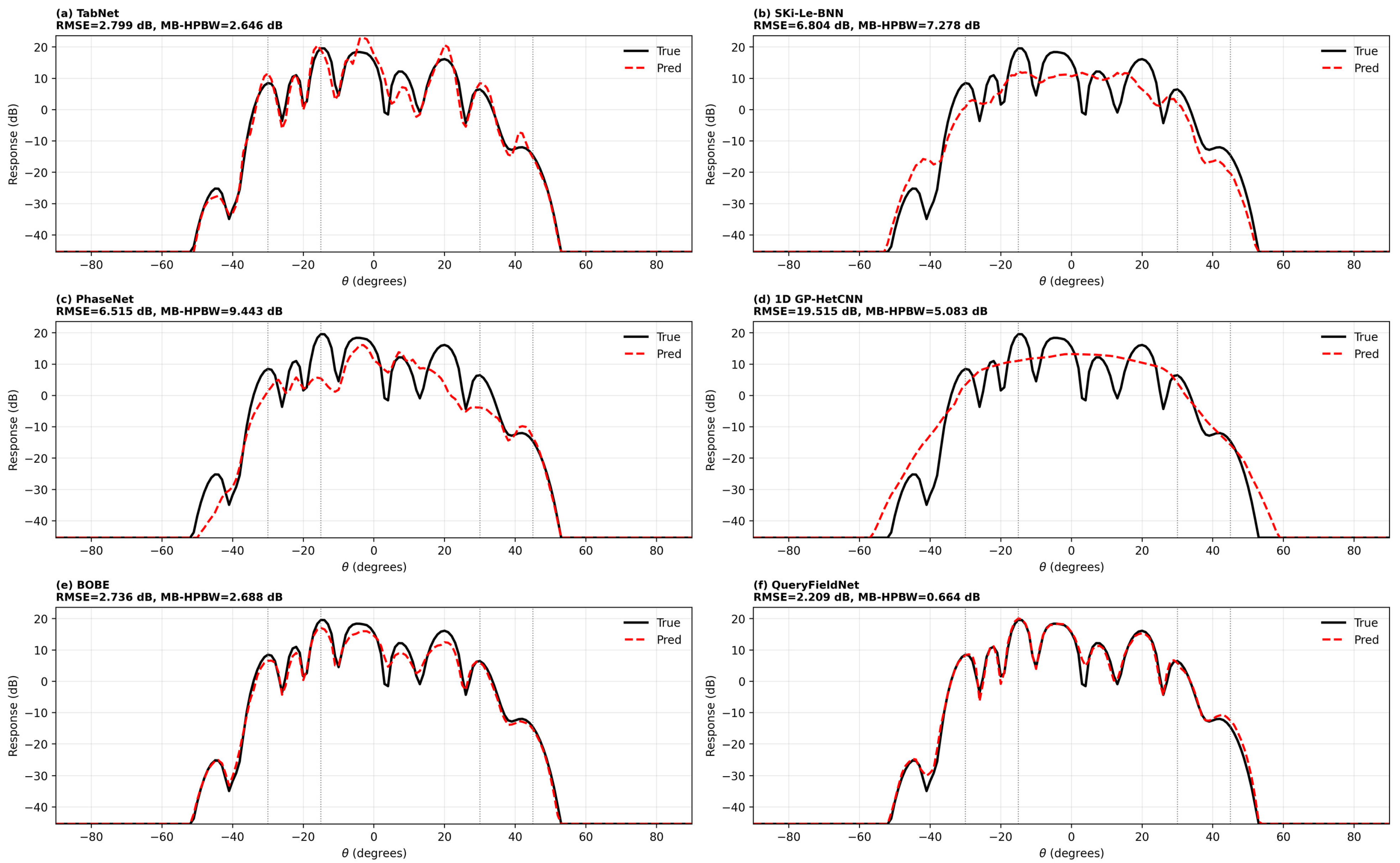
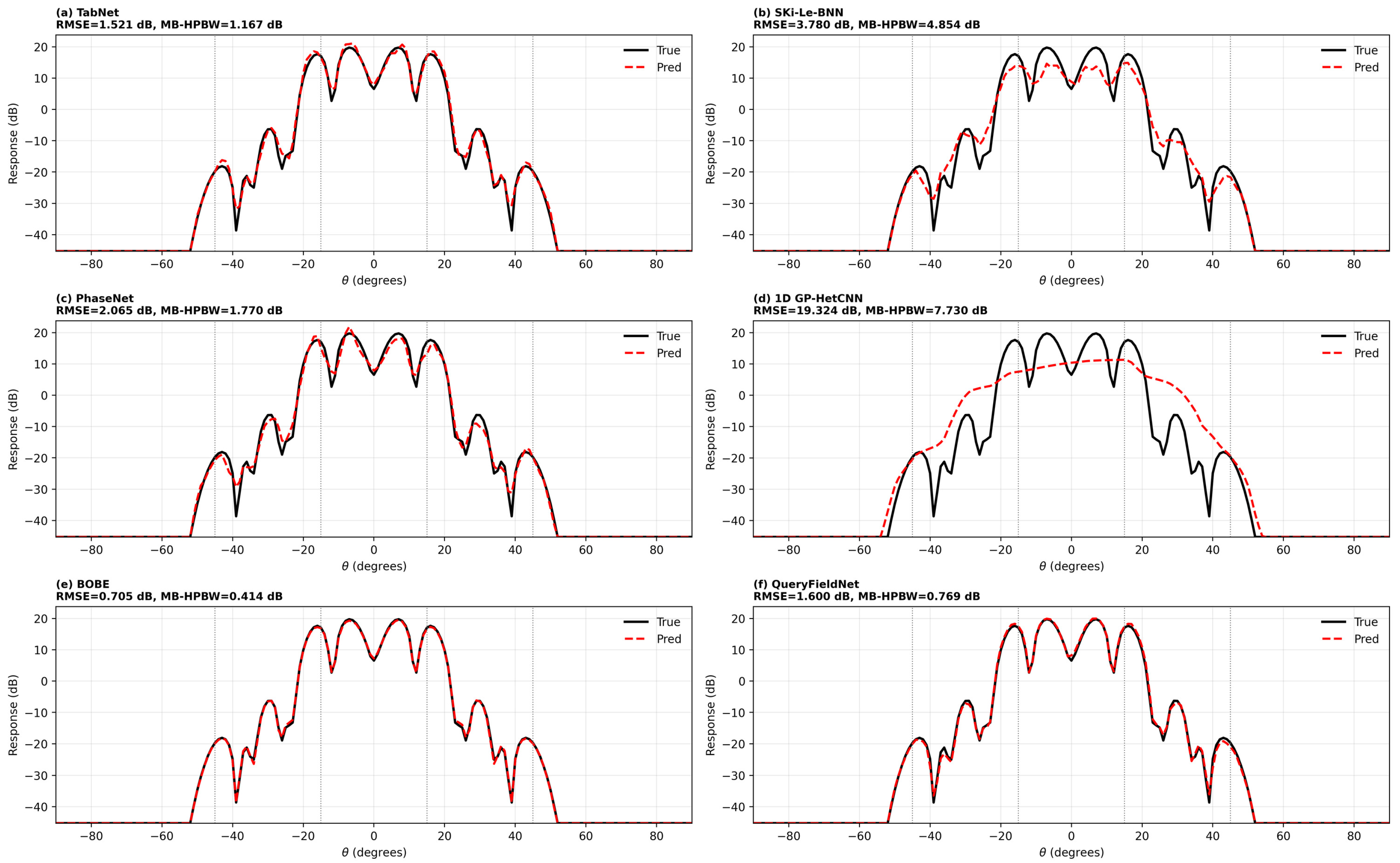
3.9. Qualitative Model Comparison
4. Discussion
5. Conclusions
Author Contributions
Funding
Institutional Review Board Statement
Informed Consent Statement
Data Availability Statement
Conflicts of Interest
Appendix A. Verified Model and Training Details

| Aspect | Adapted PhaseNet | QueryFieldNet |
|---|---|---|
| Input representation | Two-dimensional phase map with condition features | sin/cos phase channels, spatial coordinates, and bit/cut conditions |
| Output definition | Direct regression of a 181-point curve | 181 angle-conditioned query outputs |
| Angular decoding | Fixed output-vector decoder | Fourier-angle queries, cross-attention, and dilated 1D convolution |
| Intended-beam metadata | Not used | Auxiliary occupancy/count head and metadata-gated residual branch |
| Training objective | Full-curve MSE | Composite full-curve, local-region, shape, peak, and metadata losses |
| Evaluation | Global and local-window metrics under the common protocol | Same output and metric definitions |
| Setting | Value |
|---|---|
| Training scope | One joint model trained on the pooled 1-bit to 5-bit training split |
| Optimizer/batch size | AdamW/256 |
| Initial learning rate/weight decay | / |
| Maximum budget/early stopping | 15,000 epochs/patience 250; final runs stopped after 312–589 epochs |
| Learning-rate scheduler | ReduceLROnPlateau with patience 60 |
| Loss weights | , , , , , , and |
| Curriculum/teacher forcing | 180-epoch loss warm-up; occupancy teacher forcing decays from 0.2 to 0 over 500 epochs |
| Training/evaluation radius | intended-beam training region/ evaluation window |
| Checkpoint criterion | Minimum composite validation score in Equation (26) |
References
- Berry, D.G.; Malech, R.G.; Kennedy, W.A. The Reflectarray Antenna. IEEE Trans. Antennas Propag. 1963, 11, 645–651. [Google Scholar] [CrossRef] [Scilit]
- Huang, J.; Encinar, J.A. Reflectarray Antennas; IEEE Press/Wiley: Hoboken, NJ, USA, 2008. [Google Scholar] [CrossRef] [Scilit]
- Balanis, C.A. Antenna Theory: Analysis and Design, 4th ed.; Wiley: Hoboken, NJ, USA, 2016; ISBN 978-1-118-64206-1. [Google Scholar]
- Pozar, D.M.; Targonski, S.D.; Syrigos, H.D. Design of Millimeter Wave Microstrip Reflectarrays. IEEE Trans. Antennas Propag. 1997, 45, 287–296. [Google Scholar] [CrossRef] [Scilit]
- Nayeri, P.; Yang, F.; Elsherbeni, A.Z. Reflectarray Antennas: Theory, Designs, and Applications; Wiley: Hoboken, NJ, USA, 2018. [Google Scholar] [CrossRef] [Scilit]
- El Misilmani, H.M.; Naous, T.; Al Khatib, S.K. A Review on the Design and Optimization of Antennas Using Machine Learning Algorithms and Techniques. Int. J. Rf Microw.-Comput.-Aided Eng. 2020, 30, e22356. [Google Scholar] [CrossRef] [Scilit]
- Khan, M.M.; Hossain, S.; Mozumdar, P.; Akter, S.; Ashique, R.H. A Review on Machine Learning and Deep Learning for Various Antenna Design Applications. Heliyon 2022, 8, e09317. [Google Scholar] [CrossRef] [Scilit] [PubMed]
- Sarker, N.; Podder, P.; Mondal, M.R.H.; Shafin, S.S.; Kamruzzaman, J. Applications of Machine Learning and Deep Learning in Antenna Design, Optimization, and Selection: A Review. IEEE Access 2023, 11, 103890–103915. [Google Scholar] [CrossRef] [Scilit]
- Vaswani, A.; Shazeer, N.; Parmar, N.; Uszkoreit, J.; Jones, L.; Gomez, A.N.; Kaiser, Ł.; Polosukhin, I. Attention Is All You Need. Adv. Neural Inf. Process. Syst. 2017, 30, 5998–6008. [Google Scholar]
- Zhu, Z.; Tian, Y.; Sun, J. Antenna Modeling Based on Image-CNN-LSTM. IEEE Antennas Wirel. Propag. Lett. 2024, 23, 2738–2742. [Google Scholar] [CrossRef] [Scilit]
- Wei, Z.; Zhou, Z.; Wang, P.; Ren, J.; Yin, Y.; Pedersen, G.F.; Shen, M. Fast and Automatic Parametric Model Construction of Antenna Structures Using CNN-LSTM Networks. IEEE Trans. Antennas Propag. 2024, 72, 1319–1328. [Google Scholar] [CrossRef] [Scilit]
- Reddy, V.; Singh, P.; Kumar, J. A Hybrid BOBE Framework for Scattering Parameter Prediction of Wideband Crescent Slot Microstrip Antenna. Array 2026, 30, 100872. [Google Scholar] [CrossRef] [Scilit]
- Oh, S.; Pyo, S.; Jang, H. PhaseNet: A Deep Learning Framework for Reflectarray Antenna Gain Prediction by Integrating 2D Phase Maps and Angular Embeddings. Mathematics 2025, 13, 3509. [Google Scholar] [CrossRef] [Scilit]
- Mildenhall, B.; Srinivasan, P.P.; Tancik, M.; Barron, J.T.; Ramamoorthi, R.; Ng, R. NeRF: Representing Scenes as Neural Radiance Fields for View Synthesis. In Proceedings of the European Conference on Computer Vision; Springer: Cham, Switzerland, 2020; pp. 405–421. [Google Scholar] [CrossRef] [Scilit]
- Chen, Y.; Liu, S.; Wang, X. Learning Continuous Image Representation with Local Implicit Image Function. In Proceedings of the IEEE/CVF Conference on Computer Vision and Pattern Recognition, Nashville, TN, USA, 20–25 June 2021; pp. 8628–8638. [Google Scholar] [CrossRef] [Scilit]
- Carion, N.; Massa, F.; Synnaeve, G.; Usunier, N.; Kirillov, A.; Zagoruyko, S. End-to-End Object Detection with Transformers. In Proceedings of the European Conference on Computer Vision; Springer: Cham, Switzerland, 2020; pp. 213–229. [Google Scholar] [CrossRef] [Scilit]
- Jaegle, A.; Borgeaud, S.; Alayrac, J.-B.; Doersch, C.; Ionescu, C.; Ding, F.; Koppula, S.; Zoran, D.; Brock, A.; Shelhamer, E.; et al. Perceiver IO: A General Architecture for Structured Inputs & Outputs. In Proceedings of the International Conference on Learning Representations (ICLR), Virtual, 25–29 April 2022; Available online: https://iclr.cc/virtual/2022/poster/6269 (accessed on 25 April 2022).
- Arik, S.O.; Pfister, T. TabNet: Attentive Interpretable Tabular Learning. Proc. Aaai Conf. Artif. Intell. 2021, 35, 6679–6687. [Google Scholar] [CrossRef] [Scilit]
- Tian, Y.; Sun, J.; Zhu, Z. Skip-Connected CNN Exploiting BNN Surrogate for Antenna Modelling. Int. J. Antennas Propag. 2025, 2025, 4999463. [Google Scholar] [CrossRef] [Scilit]
- Yang, X.; Nan, J.; Wang, M. Antenna Modeling and Optimization Based on 1D GP-HetCNN Surrogates and Intelligent Methods. Discov. Appl. Sci. 2026, 8, 119. [Google Scholar] [CrossRef] [Scilit]
- Chen, T.; Guestrin, C. XGBoost: A Scalable Tree Boosting System. In Proceedings of the 22nd ACM SIGKDD International Conference on Knowledge Discovery and Data Mining; Association for Computing Machinery: New York, NY, USA, 2016; pp. 785–794. [Google Scholar] [CrossRef] [Scilit]
- Breiman, L. Random Forests. Mach. Learn. 2001, 45, 5–32. [Google Scholar] [CrossRef] [Scilit]
- Geurts, P.; Ernst, D.; Wehenkel, L. Extremely Randomized Trees. Mach. Learn. 2006, 63, 3–42. [Google Scholar] [CrossRef] [Scilit]
- Prokhorenkova, L.; Gusev, G.; Vorobev, A.; Dorogush, A.V.; Gulin, A. CatBoost: Unbiased Boosting with Categorical Features. Adv. Neural Inf. Process. Syst. 2018, 31, 6638–6648. [Google Scholar]
- Akiba, T.; Sano, S.; Yanase, T.; Ohta, T.; Koyama, M. Optuna: A Next-Generation Hyperparameter Optimization Framework. In Proceedings of the 25th ACM SIGKDD International Conference on Knowledge Discovery and Data Mining; Association for Computing Machinery: New York, NY, USA, 2019; pp. 2623–2631. [Google Scholar] [CrossRef] [Scilit]



| Item | Configuration |
|---|---|
| Aperture/frequency | Square reflectarray phase-map grid, 8 GHz |
| Forward-model aperture mask | Continuous square mask with side length mm; all 19 × 19 cell centers are retained in the aperture summation |
| Cell/feed | 20.1 mm unit-cell pitch, feed = (0, 0, 250) mm |
| Phase map/bit depth | 19 × 19 phase map, 1-bit to 5-bit |
| Beam condition | 1 to 4 beams, , intended-beam azimuth |
| Balanced sampling | 500 phase maps per beam count for each bit depth; positions sampled as evenly as possible |
| Output condition | principal cuts and , output to , 181 points |
| Dataset size | 2000 phase maps per bit, 4000 CSV rows per bit |
| Split | 80/10/10 at the phase-map level: 1600/200/200 phase maps (3200/400/400 cut rows) |
| Bit Depth | Model (Year) | RMSE | MAE | MB-HPBW RMSE | MB-Main-Lobe RMSE | Beam-Peak RMSE | |
|---|---|---|---|---|---|---|---|
| 1 | TabNet (2021) | 3.313 ± 0.018 | 2.169 ± 0.009 | 0.99791 ± 0.00002 | 2.501 ± 0.103 | 2.584 ± 0.091 | 2.250 ± 0.048 |
| SKi-Le-BNN (2025) | 5.060 ± 0.063 | 3.560 ± 0.084 | 0.99513 ± 0.00012 | 6.097 ± 0.097 | 5.459 ± 0.062 | 5.093 ± 0.141 | |
| PhaseNet (2025) | 3.342 ± 0.054 | 2.125 ± 0.037 | 0.99788 ± 0.00007 | 2.666 ± 0.067 | 2.661 ± 0.032 | 2.446 ± 0.203 | |
| 1D GP-HetCNN (2026) | 15.296 ± 1.799 | 10.934 ± 0.471 | 0.95511 ± 0.01069 | 6.922 ± 0.832 | 6.919 ± 0.820 | 7.250 ± 0.952 | |
| BOBE (2026) | 3.172 ± 0.036 | 1.996 ± 0.035 | 0.99809 ± 0.00004 | 2.190 ± 0.140 | 2.231 ± 0.136 | 2.066 ± 0.181 | |
| QueryFieldNet-Lite | 2.987 ± 0.036 | 1.884 ± 0.033 | 0.99830 ± 0.00004 | 1.481 ± 0.085 | 1.749 ± 0.062 | 1.468 ± 0.115 | |
| QueryFieldNet | 2.456 ± 0.200 | 1.486 ± 0.173 | 0.99885 ± 0.00018 | 1.211 ± 0.061 | 1.422 ± 0.085 | 1.041 ± 0.076 | |
| 2 | TabNet (2021) | 4.311 ± 0.032 | 3.007 ± 0.025 | 0.99640 ± 0.00005 | 3.504 ± 0.077 | 3.633 ± 0.092 | 3.108 ± 0.098 |
| SKi-Le-BNN (2025) | 5.836 ± 0.018 | 4.448 ± 0.022 | 0.99339 ± 0.00004 | 7.798 ± 0.055 | 6.868 ± 0.050 | 6.226 ± 0.042 | |
| PhaseNet (2025) | 4.289 ± 0.045 | 2.999 ± 0.023 | 0.99643 ± 0.00008 | 3.490 ± 0.046 | 3.561 ± 0.051 | 2.981 ± 0.018 | |
| 1D GP-HetCNN (2026) | 16.620 ± 2.590 | 12.958 ± 1.839 | 0.94552 ± 0.01607 | 10.615 ± 2.660 | 10.364 ± 2.417 | 10.964 ± 2.611 | |
| BOBE (2026) | 3.728 ± 0.147 | 2.536 ± 0.117 | 0.99729 ± 0.00023 | 2.770 ± 0.285 | 2.815 ± 0.227 | 2.528 ± 0.244 | |
| QueryFieldNet-Lite | 3.702 ± 0.054 | 2.432 ± 0.047 | 0.99734 ± 0.00008 | 2.028 ± 0.069 | 2.346 ± 0.053 | 2.038 ± 0.055 | |
| QueryFieldNet | 3.277 ± 0.170 | 2.074 ± 0.151 | 0.99791 ± 0.00021 | 1.709 ± 0.129 | 1.992 ± 0.128 | 1.721 ± 0.150 | |
| 3 | TabNet (2021) | 4.390 ± 0.049 | 2.995 ± 0.023 | 0.99623 ± 0.00008 | 3.715 ± 0.224 | 3.769 ± 0.145 | 3.211 ± 0.104 |
| SKi-Le-BNN (2025) | 5.623 ± 0.382 | 4.309 ± 0.315 | 0.99380 ± 0.00085 | 6.457 ± 1.283 | 5.976 ± 1.022 | 5.090 ± 0.812 | |
| PhaseNet (2025) | 4.326 ± 0.081 | 2.963 ± 0.031 | 0.99634 ± 0.00014 | 3.609 ± 0.157 | 3.677 ± 0.125 | 2.938 ± 0.048 | |
| 1D GP-HetCNN (2026) | 18.780 ± 3.291 | 14.488 ± 1.719 | 0.92956 ± 0.02383 | 11.184 ± 2.068 | 10.784 ± 2.156 | 11.376 ± 2.292 | |
| BOBE (2026) | 3.730 ± 0.041 | 2.436 ± 0.059 | 0.99727 ± 0.00006 | 2.677 ± 0.171 | 2.792 ± 0.162 | 2.431 ± 0.102 | |
| QueryFieldNet-Lite | 3.937 ± 0.078 | 2.570 ± 0.066 | 0.99697 ± 0.00012 | 2.440 ± 0.090 | 2.716 ± 0.054 | 2.223 ± 0.041 | |
| QueryFieldNet | 3.618 ± 0.159 | 2.264 ± 0.130 | 0.99744 ± 0.00022 | 2.194 ± 0.012 | 2.480 ± 0.068 | 2.030 ± 0.049 | |
| 4 | TabNet (2021) | 3.975 ± 0.084 | 2.586 ± 0.046 | 0.99690 ± 0.00013 | 3.218 ± 0.099 | 3.313 ± 0.091 | 2.748 ± 0.070 |
| SKi-Le-BNN (2025) | 4.405 ± 0.217 | 3.176 ± 0.209 | 0.99619 ± 0.00038 | 3.945 ± 0.373 | 4.094 ± 0.289 | 3.111 ± 0.239 | |
| PhaseNet (2025) | 4.026 ± 0.031 | 2.633 ± 0.037 | 0.99682 ± 0.00005 | 3.341 ± 0.055 | 3.466 ± 0.086 | 2.832 ± 0.084 | |
| 1D GP-HetCNN (2026) | 19.279 ± 3.919 | 14.266 ± 2.533 | 0.92509 ± 0.03092 | 9.758 ± 2.632 | 9.402 ± 2.472 | 9.885 ± 2.693 | |
| BOBE (2026) | 3.637 ± 0.028 | 2.232 ± 0.007 | 0.99740 ± 0.00004 | 2.634 ± 0.152 | 2.738 ± 0.161 | 2.400 ± 0.060 | |
| QueryFieldNet-Lite | 3.710 ± 0.042 | 2.362 ± 0.058 | 0.99730 ± 0.00006 | 2.420 ± 0.088 | 2.694 ± 0.077 | 2.261 ± 0.059 | |
| QueryFieldNet | 3.475 ± 0.078 | 2.098 ± 0.097 | 0.99763 ± 0.00011 | 2.229 ± 0.097 | 2.468 ± 0.041 | 1.982 ± 0.054 | |
| 5 | TabNet (2021) | 3.676 ± 0.139 | 2.240 ± 0.046 | 0.99734 ± 0.00020 | 2.584 ± 0.101 | 2.804 ± 0.097 | 2.314 ± 0.111 |
| SKi-Le-BNN (2025) | 3.683 ± 0.122 | 2.399 ± 0.125 | 0.99733 ± 0.00018 | 2.749 ± 0.172 | 2.998 ± 0.177 | 2.248 ± 0.126 | |
| PhaseNet (2025) | 3.705 ± 0.022 | 2.303 ± 0.024 | 0.99730 ± 0.00003 | 2.518 ± 0.048 | 2.820 ± 0.059 | 2.235 ± 0.068 | |
| 1D GP-HetCNN (2026) | 24.217 ± 3.765 | 17.433 ± 2.546 | 0.88302 ± 0.03477 | 9.329 ± 0.322 | 9.052 ± 0.302 | 9.393 ± 0.346 | |
| BOBE (2026) | 3.195 ± 0.111 | 1.824 ± 0.061 | 0.99799 ± 0.00014 | 2.247 ± 0.248 | 2.353 ± 0.117 | 1.839 ± 0.107 | |
| QueryFieldNet-Lite | 3.594 ± 0.085 | 2.204 ± 0.047 | 0.99746 ± 0.00012 | 2.042 ± 0.138 | 2.375 ± 0.115 | 2.041 ± 0.026 | |
| QueryFieldNet | 3.375 ± 0.130 | 1.954 ± 0.127 | 0.99776 ± 0.00017 | 2.018 ± 0.076 | 2.307 ± 0.105 | 1.876 ± 0.046 | |
| Mean | TabNet (2021) | 3.933 ± 0.034 | 2.599 ± 0.008 | 0.99696 ± 0.00005 | 3.104 ± 0.009 | 3.221 ± 0.019 | 2.726 ± 0.015 |
| SKi-Le-BNN (2025) | 4.922 ± 0.091 | 3.579 ± 0.085 | 0.99517 ± 0.00020 | 5.409 ± 0.294 | 5.079 ± 0.231 | 4.354 ± 0.136 | |
| PhaseNet (2025) | 3.938 ± 0.033 | 2.605 ± 0.018 | 0.99695 ± 0.00005 | 3.125 ± 0.029 | 3.237 ± 0.016 | 2.687 ± 0.042 | |
| 1D GP-HetCNN (2026) | 18.838 ± 1.950 | 14.016 ± 1.043 | 0.92766 ± 0.01517 | 9.562 ± 0.934 | 9.304 ± 0.837 | 9.774 ± 0.980 | |
| BOBE (2026) | 3.492 ± 0.003 | 2.205 ± 0.015 | 0.99761 ± 0.00001 | 2.504 ± 0.081 | 2.586 ± 0.038 | 2.253 ± 0.050 | |
| QueryFieldNet-Lite | 3.586 ± 0.050 | 2.290 ± 0.049 | 0.99747 ± 0.00007 | 2.082 ± 0.078 | 2.376 ± 0.065 | 2.006 ± 0.038 | |
| QueryFieldNet | 3.240 ± 0.143 | 1.975 ± 0.134 | 0.99792 ± 0.00017 | 1.872 ± 0.015 | 2.134 ± 0.047 | 1.730 ± 0.065 |
| (a) | |||||||
|---|---|---|---|---|---|---|---|
| Beam Count | Model (Year) | RMSE | MAE | MB-HPBW RMSE | MB-Main-Lobe RMSE | Beam-Peak RMSE | |
| 1 | TabNet (2021) | 3.008 ± 0.075 | 1.975 ± 0.039 | 0.99827 ± 0.00009 | 2.295 ± 0.135 | 2.390 ± 0.061 | 1.920 ± 0.023 |
| SKi-Le-BNN (2025) | 5.194 ± 0.067 | 3.642 ± 0.081 | 0.99484 ± 0.00013 | 9.422 ± 0.113 | 8.597 ± 0.108 | 6.848 ± 0.142 | |
| PhaseNet (2025) | 2.875 ± 0.018 | 1.826 ± 0.040 | 0.99842 ± 0.00002 | 2.132 ± 0.148 | 2.189 ± 0.136 | 1.811 ± 0.097 | |
| 1D GP-HetCNN (2026) | 15.176 ± 1.871 | 10.866 ± 0.519 | 0.95599 ± 0.01071 | 7.428 ± 0.298 | 7.339 ± 0.321 | 7.505 ± 0.428 | |
| BOBE (2026) | 2.510 ± 0.274 | 1.529 ± 0.236 | 0.99878 ± 0.00027 | 1.949 ± 0.204 | 1.917 ± 0.103 | 1.663 ± 0.127 | |
| QueryFieldNet-Lite | 2.693 ± 0.070 | 1.671 ± 0.057 | 0.99861 ± 0.00007 | 1.127 ± 0.121 | 1.295 ± 0.118 | 1.149 ± 0.162 | |
| QueryFieldNet | 2.350 ± 0.083 | 1.431 ± 0.063 | 0.99894 ± 0.00007 | 1.041 ± 0.082 | 1.232 ± 0.095 | 1.043 ± 0.051 | |
| 2 | TabNet (2021) | 3.435 ± 0.079 | 2.264 ± 0.040 | 0.99776 ± 0.00010 | 2.428 ± 0.162 | 2.521 ± 0.187 | 2.267 ± 0.163 |
| SKi-Le-BNN (2025) | 5.321 ± 0.061 | 3.768 ± 0.080 | 0.99462 ± 0.00012 | 6.658 ± 0.087 | 5.901 ± 0.051 | 5.593 ± 0.145 | |
| PhaseNet (2025) | 3.298 ± 0.038 | 2.171 ± 0.007 | 0.99793 ± 0.00005 | 2.636 ± 0.119 | 2.551 ± 0.084 | 2.271 ± 0.092 | |
| 1D GP-HetCNN (2026) | 15.782 ± 1.833 | 11.230 ± 0.452 | 0.95246 ± 0.01114 | 7.248 ± 0.644 | 7.175 ± 0.612 | 7.515 ± 0.733 | |
| BOBE (2026) | 3.467 ± 0.148 | 2.149 ± 0.183 | 0.99772 ± 0.00020 | 2.341 ± 0.295 | 2.319 ± 0.129 | 1.988 ± 0.263 | |
| QueryFieldNet-Lite | 3.111 ± 0.031 | 1.996 ± 0.014 | 0.99816 ± 0.00004 | 1.536 ± 0.019 | 1.800 ± 0.044 | 1.530 ± 0.078 | |
| QueryFieldNet | 2.781 ± 0.045 | 1.757 ± 0.020 | 0.99853 ± 0.00005 | 1.385 ± 0.111 | 1.668 ± 0.125 | 1.342 ± 0.094 | |
| 3 | TabNet (2021) | 3.604 ± 0.029 | 2.353 ± 0.030 | 0.99754 ± 0.00004 | 2.873 ± 0.064 | 2.848 ± 0.030 | 2.408 ± 0.048 |
| SKi-Le-BNN (2025) | 5.011 ± 0.068 | 3.553 ± 0.087 | 0.99524 ± 0.00013 | 5.761 ± 0.095 | 5.016 ± 0.064 | 4.868 ± 0.150 | |
| PhaseNet (2025) | 3.780 ± 0.278 | 2.422 ± 0.125 | 0.99728 ± 0.00041 | 3.098 ± 0.120 | 2.978 ± 0.069 | 2.785 ± 0.158 | |
| 1D GP-HetCNN (2026) | 15.295 ± 1.762 | 10.960 ± 0.513 | 0.95504 ± 0.01076 | 6.841 ± 0.768 | 6.819 ± 0.784 | 7.225 ± 0.885 | |
| BOBE (2026) | 3.343 ± 0.250 | 2.193 ± 0.199 | 0.99787 ± 0.00032 | 2.137 ± 0.340 | 2.252 ± 0.274 | 2.089 ± 0.369 | |
| QueryFieldNet-Lite | 3.190 ± 0.080 | 2.037 ± 0.050 | 0.99807 ± 0.00010 | 1.641 ± 0.162 | 1.935 ± 0.112 | 1.566 ± 0.163 | |
| QueryFieldNet | 2.949 ± 0.137 | 1.854 ± 0.085 | 0.99835 ± 0.00015 | 1.427 ± 0.107 | 1.783 ± 0.106 | 1.422 ± 0.168 | |
| 4 | TabNet (2021) | 3.270 ± 0.056 | 2.146 ± 0.045 | 0.99797 ± 0.00007 | 2.342 ± 0.093 | 2.480 ± 0.102 | 2.225 ± 0.059 |
| SKi-Le-BNN (2025) | 4.549 ± 0.060 | 3.185 ± 0.095 | 0.99608 ± 0.00010 | 4.317 ± 0.123 | 3.928 ± 0.082 | 4.070 ± 0.140 | |
| PhaseNet (2025) | 3.544 ± 0.205 | 2.204 ± 0.030 | 0.99761 ± 0.00028 | 2.529 ± 0.035 | 2.624 ± 0.093 | 2.450 ± 0.543 | |
| 1D GP-HetCNN (2026) | 14.919 ± 1.742 | 10.681 ± 0.407 | 0.95693 ± 0.01024 | 6.676 ± 1.142 | 6.750 ± 1.093 | 7.056 ± 1.274 | |
| BOBE (2026) | 3.263 ± 0.106 | 2.095 ± 0.135 | 0.99798 ± 0.00014 | 2.178 ± 0.183 | 2.219 ± 0.222 | 2.128 ± 0.229 | |
| QueryFieldNet-Lite | 3.021 ± 0.073 | 1.898 ± 0.040 | 0.99827 ± 0.00008 | 1.431 ± 0.062 | 1.713 ± 0.051 | 1.451 ± 0.124 | |
| QueryFieldNet | 2.767 ± 0.117 | 1.723 ± 0.099 | 0.99855 ± 0.00012 | 1.194 ± 0.021 | 1.519 ± 0.016 | 1.265 ± 0.056 | |
| (b) | |||||||
| Beam Count | Model (Year) | RMSE | MAE | MB-HPBW RMSE | MB-Main-Lobe RMSE | Beam-Peak RMSE | |
| 1 | TabNet (2021) | 3.869 ± 0.014 | 2.720 ± 0.020 | 0.99708 ± 0.00002 | 3.295 ± 0.173 | 3.256 ± 0.100 | 3.161 ± 0.222 |
| SKi-Le-BNN (2025) | 5.810 ± 0.022 | 4.292 ± 0.031 | 0.99341 ± 0.00005 | 12.192 ± 0.196 | 10.941 ± 0.190 | 8.002 ± 0.130 | |
| PhaseNet (2025) | 3.767 ± 0.083 | 2.609 ± 0.058 | 0.99723 ± 0.00012 | 2.606 ± 0.126 | 2.827 ± 0.069 | 2.489 ± 0.165 | |
| 1D GP-HetCNN (2026) | 16.533 ± 2.543 | 13.010 ± 1.912 | 0.94550 ± 0.01560 | 11.297 ± 2.662 | 10.832 ± 2.420 | 11.346 ± 2.817 | |
| BOBE (2026) | 3.534 ± 0.047 | 2.373 ± 0.081 | 0.99754 ± 0.00007 | 2.565 ± 0.920 | 2.684 ± 0.650 | 2.521 ± 0.812 | |
| QueryFieldNet-Lite | 3.465 ± 0.107 | 2.279 ± 0.086 | 0.99765 ± 0.00015 | 1.758 ± 0.188 | 1.999 ± 0.143 | 2.016 ± 0.273 | |
| QueryFieldNet | 3.229 ± 0.039 | 2.081 ± 0.009 | 0.99796 ± 0.00005 | 1.655 ± 0.190 | 1.947 ± 0.140 | 1.766 ± 0.335 | |
| 2 | TabNet (2021) | 4.206 ± 0.105 | 2.943 ± 0.071 | 0.99658 ± 0.00017 | 3.045 ± 0.107 | 3.291 ± 0.164 | 2.797 ± 0.091 |
| SKi-Le-BNN (2025) | 6.011 ± 0.011 | 4.526 ± 0.008 | 0.99301 ± 0.00003 | 8.279 ± 0.072 | 7.283 ± 0.071 | 6.657 ± 0.055 | |
| PhaseNet (2025) | 4.273 ± 0.047 | 2.979 ± 0.026 | 0.99647 ± 0.00008 | 3.201 ± 0.152 | 3.389 ± 0.187 | 2.870 ± 0.181 | |
| 1D GP-HetCNN (2026) | 16.691 ± 2.832 | 12.983 ± 1.979 | 0.94519 ± 0.01789 | 11.089 ± 2.826 | 10.747 ± 2.553 | 11.477 ± 2.803 | |
| BOBE (2026) | 3.858 ± 0.307 | 2.562 ± 0.197 | 0.99710 ± 0.00048 | 2.613 ± 0.337 | 2.696 ± 0.330 | 2.378 ± 0.265 | |
| QueryFieldNet-Lite | 3.751 ± 0.021 | 2.465 ± 0.029 | 0.99728 ± 0.00003 | 1.932 ± 0.094 | 2.373 ± 0.101 | 2.019 ± 0.074 | |
| QueryFieldNet | 3.475 ± 0.077 | 2.267 ± 0.054 | 0.99766 ± 0.00010 | 1.898 ± 0.120 | 2.245 ± 0.071 | 2.020 ± 0.102 | |
| 3 | TabNet (2021) | 4.395 ± 0.165 | 3.051 ± 0.104 | 0.99625 ± 0.00028 | 3.318 ± 0.114 | 3.443 ± 0.204 | 2.932 ± 0.074 |
| SKi-Le-BNN (2025) | 5.823 ± 0.024 | 4.470 ± 0.042 | 0.99343 ± 0.00006 | 7.189 ± 0.057 | 6.377 ± 0.054 | 5.969 ± 0.027 | |
| PhaseNet (2025) | 4.406 ± 0.024 | 3.096 ± 0.031 | 0.99624 ± 0.00004 | 3.554 ± 0.125 | 3.618 ± 0.035 | 2.976 ± 0.101 | |
| 1D GP-HetCNN (2026) | 16.567 ± 2.554 | 12.879 ± 1.810 | 0.94569 ± 0.01609 | 10.421 ± 2.594 | 10.242 ± 2.359 | 10.792 ± 2.490 | |
| BOBE (2026) | 3.834 ± 0.218 | 2.669 ± 0.117 | 0.99713 ± 0.00033 | 2.958 ± 0.216 | 2.980 ± 0.107 | 2.664 ± 0.131 | |
| QueryFieldNet-Lite | 3.764 ± 0.082 | 2.472 ± 0.040 | 0.99725 ± 0.00012 | 1.977 ± 0.081 | 2.271 ± 0.013 | 2.125 ± 0.131 | |
| QueryFieldNet | 3.589 ± 0.127 | 2.333 ± 0.092 | 0.99750 ± 0.00018 | 1.927 ± 0.029 | 2.232 ± 0.077 | 2.035 ± 0.079 | |
| 4 | TabNet (2021) | 4.681 ± 0.041 | 3.281 ± 0.046 | 0.99576 ± 0.00007 | 3.912 ± 0.095 | 4.010 ± 0.037 | 3.356 ± 0.167 |
| SKi-Le-BNN (2025) | 5.713 ± 0.020 | 4.495 ± 0.012 | 0.99369 ± 0.00004 | 6.441 ± 0.080 | 5.716 ± 0.052 | 5.744 ± 0.115 | |
| PhaseNet (2025) | 4.611 ± 0.109 | 3.269 ± 0.060 | 0.99589 ± 0.00019 | 3.769 ± 0.053 | 3.743 ± 0.072 | 3.131 ± 0.111 | |
| 1D GP-HetCNN (2026) | 16.680 ± 2.472 | 12.961 ± 1.717 | 0.94567 ± 0.01510 | 10.343 ± 2.621 | 10.146 ± 2.391 | 10.731 ± 2.548 | |
| BOBE (2026) | 3.686 ± 0.099 | 2.527 ± 0.129 | 0.99738 ± 0.00015 | 2.709 ± 0.391 | 2.736 ± 0.341 | 2.429 ± 0.508 | |
| QueryFieldNet-Lite | 3.797 ± 0.038 | 2.500 ± 0.045 | 0.99721 ± 0.00006 | 2.183 ± 0.101 | 2.479 ± 0.079 | 1.972 ± 0.072 | |
| QueryFieldNet | 3.717 ± 0.071 | 2.403 ± 0.047 | 0.99733 ± 0.00010 | 2.001 ± 0.064 | 2.293 ± 0.027 | 1.962 ± 0.159 | |
| (c) | |||||||
| Beam Count | Model (Year) | RMSE | MAE | MB-HPBW RMSE | MB-Main-Lobe RMSE | Beam-Peak RMSE | |
| 1 | TabNet (2021) | 4.205 ± 0.128 | 2.949 ± 0.068 | 0.99651 ± 0.00021 | 3.404 ± 0.266 | 3.708 ± 0.287 | 3.117 ± 0.300 |
| SKi-Le-BNN (2025) | 5.110 ± 0.534 | 3.861 ± 0.378 | 0.99481 ± 0.00110 | 8.539 ± 3.428 | 8.036 ± 2.815 | 6.600 ± 1.814 | |
| PhaseNet (2025) | 3.927 ± 0.080 | 2.707 ± 0.043 | 0.99696 ± 0.00012 | 2.728 ± 0.063 | 3.084 ± 0.041 | 2.590 ± 0.037 | |
| 1D GP-HetCNN (2026) | 17.997 ± 3.748 | 13.826 ± 1.864 | 0.93483 ± 0.02622 | 12.619 ± 1.342 | 11.860 ± 1.287 | 12.532 ± 1.669 | |
| BOBE (2026) | 3.627 ± 0.170 | 2.440 ± 0.182 | 0.99739 ± 0.00024 | 2.330 ± 0.360 | 2.502 ± 0.242 | 2.331 ± 0.574 | |
| QueryFieldNet-Lite | 3.550 ± 0.133 | 2.396 ± 0.087 | 0.99751 ± 0.00019 | 1.532 ± 0.102 | 2.030 ± 0.037 | 1.613 ± 0.112 | |
| QueryFieldNet | 3.313 ± 0.041 | 2.204 ± 0.037 | 0.99783 ± 0.00005 | 1.543 ± 0.124 | 2.027 ± 0.170 | 1.730 ± 0.098 | |
| 2 | TabNet (2021) | 4.422 ± 0.172 | 2.991 ± 0.092 | 0.99617 ± 0.00029 | 3.941 ± 0.373 | 4.037 ± 0.211 | 3.330 ± 0.211 |
| SKi-Le-BNN (2025) | 5.785 ± 0.361 | 4.493 ± 0.308 | 0.99343 ± 0.00083 | 7.024 ± 1.309 | 6.620 ± 1.065 | 5.576 ± 0.922 | |
| PhaseNet (2025) | 4.334 ± 0.131 | 2.946 ± 0.067 | 0.99632 ± 0.00022 | 3.508 ± 0.203 | 3.747 ± 0.244 | 3.027 ± 0.130 | |
| 1D GP-HetCNN (2026) | 18.890 ± 3.167 | 14.545 ± 1.650 | 0.92844 ± 0.02386 | 11.523 ± 2.214 | 11.136 ± 2.286 | 11.630 ± 2.391 | |
| BOBE (2026) | 3.803 ± 0.078 | 2.433 ± 0.056 | 0.99716 ± 0.00011 | 2.740 ± 0.199 | 2.806 ± 0.259 | 2.563 ± 0.287 | |
| QueryFieldNet-Lite | 4.028 ± 0.079 | 2.609 ± 0.075 | 0.99682 ± 0.00013 | 2.552 ± 0.122 | 2.844 ± 0.100 | 2.483 ± 0.141 | |
| QueryFieldNet | 4.012 ± 0.093 | 2.543 ± 0.082 | 0.99685 ± 0.00015 | 2.452 ± 0.160 | 2.768 ± 0.152 | 2.381 ± 0.227 | |
| 3 | TabNet (2021) | 4.424 ± 0.052 | 3.017 ± 0.038 | 0.99618 ± 0.00009 | 3.615 ± 0.195 | 3.721 ± 0.157 | 3.237 ± 0.060 |
| SKi-Le-BNN (2025) | 5.609 ± 0.381 | 4.322 ± 0.313 | 0.99384 ± 0.00084 | 6.043 ± 1.166 | 5.620 ± 0.937 | 4.758 ± 0.716 | |
| PhaseNet (2025) | 4.466 ± 0.102 | 3.074 ± 0.060 | 0.99610 ± 0.00018 | 3.626 ± 0.115 | 3.680 ± 0.116 | 2.955 ± 0.169 | |
| 1D GP-HetCNN (2026) | 18.945 ± 3.403 | 14.667 ± 1.872 | 0.92823 ± 0.02446 | 10.825 ± 2.178 | 10.474 ± 2.225 | 11.076 ± 2.354 | |
| BOBE (2026) | 3.752 ± 0.132 | 2.406 ± 0.085 | 0.99724 ± 0.00020 | 2.576 ± 0.479 | 2.672 ± 0.268 | 2.345 ± 0.193 | |
| QueryFieldNet-Lite | 3.926 ± 0.110 | 2.558 ± 0.079 | 0.99699 ± 0.00017 | 2.349 ± 0.095 | 2.645 ± 0.101 | 2.228 ± 0.042 | |
| QueryFieldNet | 3.786 ± 0.117 | 2.452 ± 0.089 | 0.99720 ± 0.00017 | 2.179 ± 0.074 | 2.633 ± 0.121 | 2.195 ± 0.117 | |
| 4 | TabNet (2021) | 4.453 ± 0.064 | 3.012 ± 0.033 | 0.99614 ± 0.00011 | 3.728 ± 0.278 | 3.672 ± 0.226 | 3.142 ± 0.148 |
| SKi-Le-BNN (2025) | 5.835 ± 0.305 | 4.448 ± 0.277 | 0.99336 ± 0.00070 | 5.886 ± 0.721 | 5.393 ± 0.561 | 4.752 ± 0.591 | |
| PhaseNet (2025) | 4.446 ± 0.069 | 3.051 ± 0.024 | 0.99615 ± 0.00012 | 3.809 ± 0.237 | 3.741 ± 0.108 | 2.937 ± 0.065 | |
| 1D GP-HetCNN (2026) | 19.241 ± 2.939 | 14.908 ± 1.634 | 0.92678 ± 0.02139 | 10.876 ± 2.195 | 10.533 ± 2.344 | 11.150 ± 2.432 | |
| BOBE (2026) | 3.762 ± 0.055 | 2.493 ± 0.042 | 0.99723 ± 0.00007 | 2.815 ± 0.167 | 2.945 ± 0.159 | 2.444 ± 0.257 | |
| QueryFieldNet-Lite | 4.126 ± 0.035 | 2.674 ± 0.048 | 0.99669 ± 0.00006 | 2.608 ± 0.153 | 2.827 ± 0.084 | 2.177 ± 0.115 | |
| QueryFieldNet | 3.963 ± 0.092 | 2.495 ± 0.048 | 0.99694 ± 0.00014 | 2.452 ± 0.167 | 2.645 ± 0.098 | 2.231 ± 0.098 | |
| (d) | |||||||
| Beam Count | Model (Year) | RMSE | MAE | MB-HPBW RMSE | MB-Main-Lobe RMSE | Beam-Peak RMSE | |
| 1 | TabNet (2021) | 3.621 ± 0.064 | 2.361 ± 0.045 | 0.99740 ± 0.00009 | 2.194 ± 0.303 | 2.318 ± 0.198 | 2.019 ± 0.326 |
| SKi-Le-BNN (2025) | 3.740 ± 0.087 | 2.621 ± 0.089 | 0.99723 ± 0.00013 | 3.117 ± 0.326 | 3.252 ± 0.292 | 2.272 ± 0.205 | |
| PhaseNet (2025) | 3.701 ± 0.153 | 2.362 ± 0.087 | 0.99728 ± 0.00022 | 3.130 ± 0.190 | 3.051 ± 0.191 | 2.692 ± 0.237 | |
| 1D GP-HetCNN (2026) | 18.737 ± 4.048 | 13.691 ± 2.425 | 0.92835 ± 0.03091 | 12.007 ± 3.468 | 11.417 ± 3.326 | 11.751 ± 3.639 | |
| BOBE (2026) | 3.628 ± 0.197 | 2.286 ± 0.181 | 0.99737 ± 0.00030 | 2.139 ± 0.184 | 2.584 ± 0.037 | 2.312 ± 0.274 | |
| QueryFieldNet-Lite | 3.458 ± 0.031 | 2.184 ± 0.055 | 0.99763 ± 0.00004 | 1.799 ± 0.155 | 2.049 ± 0.186 | 1.998 ± 0.290 | |
| QueryFieldNet | 3.321 ± 0.081 | 2.036 ± 0.026 | 0.99782 ± 0.00011 | 1.856 ± 0.143 | 2.137 ± 0.197 | 1.883 ± 0.178 | |
| 2 | TabNet (2021) | 4.192 ± 0.109 | 2.751 ± 0.047 | 0.99654 ± 0.00018 | 3.652 ± 0.321 | 3.581 ± 0.325 | 3.109 ± 0.075 |
| SKi-Le-BNN (2025) | 4.504 ± 0.261 | 3.307 ± 0.272 | 0.99600 ± 0.00047 | 4.063 ± 0.375 | 4.058 ± 0.258 | 3.276 ± 0.092 | |
| PhaseNet (2025) | 4.176 ± 0.072 | 2.743 ± 0.052 | 0.99657 ± 0.00012 | 3.863 ± 0.113 | 3.715 ± 0.173 | 3.188 ± 0.139 | |
| 1D GP-HetCNN (2026) | 19.018 ± 3.936 | 14.093 ± 2.510 | 0.92666 ± 0.03130 | 9.990 ± 2.893 | 9.637 ± 2.740 | 10.030 ± 3.044 | |
| BOBE (2026) | 4.008 ± 0.066 | 2.451 ± 0.083 | 0.99685 ± 0.00012 | 3.448 ± 0.429 | 3.425 ± 0.280 | 2.984 ± 0.445 | |
| QueryFieldNet-Lite | 3.966 ± 0.083 | 2.574 ± 0.058 | 0.99691 ± 0.00013 | 2.916 ± 0.062 | 2.898 ± 0.053 | 2.711 ± 0.114 | |
| QueryFieldNet | 3.847 ± 0.090 | 2.398 ± 0.049 | 0.99709 ± 0.00014 | 2.581 ± 0.250 | 2.654 ± 0.165 | 2.438 ± 0.211 | |
| 3 | TabNet (2021) | 3.984 ± 0.043 | 2.628 ± 0.023 | 0.99689 ± 0.00007 | 3.396 ± 0.040 | 3.577 ± 0.032 | 3.038 ± 0.206 |
| SKi-Le-BNN (2025) | 4.573 ± 0.287 | 3.327 ± 0.262 | 0.99589 ± 0.00052 | 3.956 ± 0.401 | 4.170 ± 0.307 | 3.095 ± 0.238 | |
| PhaseNet (2025) | 4.022 ± 0.097 | 2.673 ± 0.087 | 0.99683 ± 0.00015 | 3.342 ± 0.089 | 3.680 ± 0.052 | 3.029 ± 0.076 | |
| 1D GP-HetCNN (2026) | 19.620 ± 3.903 | 14.590 ± 2.569 | 0.92301 ± 0.03084 | 9.488 ± 2.539 | 9.124 ± 2.410 | 9.662 ± 2.627 | |
| BOBE (2026) | 3.532 ± 0.256 | 2.152 ± 0.134 | 0.99754 ± 0.00035 | 2.545 ± 0.318 | 2.735 ± 0.221 | 2.474 ± 0.255 | |
| QueryFieldNet-Lite | 3.677 ± 0.055 | 2.335 ± 0.081 | 0.99735 ± 0.00008 | 2.391 ± 0.246 | 2.873 ± 0.154 | 2.222 ± 0.129 | |
| QueryFieldNet | 3.570 ± 0.110 | 2.218 ± 0.078 | 0.99750 ± 0.00015 | 2.023 ± 0.137 | 2.601 ± 0.186 | 1.963 ± 0.082 | |
| 4 | TabNet (2021) | 4.065 ± 0.212 | 2.608 ± 0.111 | 0.99679 ± 0.00033 | 3.081 ± 0.034 | 3.174 ± 0.046 | 2.521 ± 0.142 |
| SKi-Le-BNN (2025) | 4.684 ± 0.217 | 3.408 ± 0.216 | 0.99574 ± 0.00040 | 4.062 ± 0.369 | 4.206 ± 0.293 | 3.201 ± 0.322 | |
| PhaseNet (2025) | 4.163 ± 0.085 | 2.737 ± 0.077 | 0.99664 ± 0.00014 | 3.115 ± 0.057 | 3.284 ± 0.111 | 2.572 ± 0.049 | |
| 1D GP-HetCNN (2026) | 19.710 ± 3.867 | 14.686 ± 2.677 | 0.92242 ± 0.03099 | 9.208 ± 2.328 | 8.929 ± 2.142 | 9.446 ± 2.293 | |
| BOBE (2026) | 3.409 ± 0.158 | 2.086 ± 0.117 | 0.99774 ± 0.00021 | 2.312 ± 0.315 | 2.368 ± 0.245 | 2.021 ± 0.211 | |
| QueryFieldNet-Lite | 3.728 ± 0.068 | 2.362 ± 0.059 | 0.99730 ± 0.00010 | 2.304 ± 0.098 | 2.591 ± 0.120 | 2.132 ± 0.056 | |
| QueryFieldNet | 3.518 ± 0.123 | 2.149 ± 0.067 | 0.99760 ± 0.00017 | 2.084 ± 0.019 | 2.395 ± 0.038 | 2.109 ± 0.061 | |
| (e) | |||||||
| Beam Count | Model (Year) | RMSE | MAE | MB-HPBW RMSE | MB-Main-Lobe RMSE | Beam-Peak RMSE | |
| 1 | TabNet (2021) | 3.710 ± 0.132 | 2.200 ± 0.020 | 0.99726 ± 0.00020 | 2.091 ± 0.102 | 2.528 ± 0.144 | 2.386 ± 0.090 |
| SKi-Le-BNN (2025) | 3.586 ± 0.076 | 2.209 ± 0.065 | 0.99744 ± 0.00011 | 2.476 ± 0.288 | 2.739 ± 0.175 | 2.529 ± 0.156 | |
| PhaseNet (2025) | 3.698 ± 0.082 | 2.204 ± 0.041 | 0.99728 ± 0.00012 | 2.127 ± 0.106 | 2.694 ± 0.078 | 2.148 ± 0.062 | |
| 1D GP-HetCNN (2026) | 23.585 ± 3.879 | 16.843 ± 2.638 | 0.88743 ± 0.03510 | 11.579 ± 0.522 | 11.054 ± 0.466 | 11.323 ± 0.452 | |
| BOBE (2026) | 3.568 ± 0.277 | 2.113 ± 0.207 | 0.99746 ± 0.00039 | 1.850 ± 0.154 | 2.288 ± 0.394 | 1.661 ± 0.307 | |
| QueryFieldNet-Lite | 3.733 ± 0.104 | 2.255 ± 0.062 | 0.99723 ± 0.00015 | 1.951 ± 0.099 | 2.414 ± 0.066 | 2.294 ± 0.108 | |
| QueryFieldNet | 3.592 ± 0.035 | 2.098 ± 0.039 | 0.99743 ± 0.00005 | 1.911 ± 0.053 | 2.289 ± 0.014 | 2.303 ± 0.156 | |
| 2 | TabNet (2021) | 3.587 ± 0.172 | 2.156 ± 0.065 | 0.99747 ± 0.00024 | 2.712 ± 0.123 | 3.054 ± 0.083 | 2.506 ± 0.132 |
| SKi-Le-BNN (2025) | 3.633 ± 0.086 | 2.372 ± 0.121 | 0.99741 ± 0.00012 | 2.767 ± 0.174 | 3.179 ± 0.154 | 2.420 ± 0.120 | |
| PhaseNet (2025) | 3.586 ± 0.071 | 2.224 ± 0.041 | 0.99748 ± 0.00010 | 2.564 ± 0.112 | 3.026 ± 0.116 | 2.594 ± 0.189 | |
| 1D GP-HetCNN (2026) | 24.162 ± 3.812 | 17.515 ± 2.604 | 0.88409 ± 0.03574 | 9.776 ± 0.425 | 9.519 ± 0.373 | 9.754 ± 0.437 | |
| BOBE (2026) | 3.174 ± 0.147 | 1.772 ± 0.116 | 0.99801 ± 0.00020 | 2.203 ± 0.424 | 2.530 ± 0.311 | 2.054 ± 0.409 | |
| QueryFieldNet-Lite | 3.581 ± 0.093 | 2.179 ± 0.026 | 0.99748 ± 0.00013 | 2.236 ± 0.202 | 2.688 ± 0.139 | 2.293 ± 0.014 | |
| QueryFieldNet | 3.450 ± 0.061 | 2.021 ± 0.031 | 0.99766 ± 0.00008 | 2.188 ± 0.019 | 2.738 ± 0.077 | 2.271 ± 0.054 | |
| 3 | TabNet (2021) | 3.932 ± 0.166 | 2.407 ± 0.055 | 0.99697 ± 0.00025 | 2.761 ± 0.144 | 2.854 ± 0.158 | 2.036 ± 0.203 |
| SKi-Le-BNN (2025) | 3.870 ± 0.192 | 2.550 ± 0.179 | 0.99706 ± 0.00030 | 2.848 ± 0.182 | 2.968 ± 0.205 | 2.021 ± 0.147 | |
| PhaseNet (2025) | 3.918 ± 0.148 | 2.458 ± 0.069 | 0.99699 ± 0.00023 | 2.684 ± 0.112 | 2.776 ± 0.112 | 1.900 ± 0.051 | |
| 1D GP-HetCNN (2026) | 24.375 ± 3.713 | 17.553 ± 2.503 | 0.88164 ± 0.03409 | 9.019 ± 0.366 | 8.744 ± 0.367 | 9.090 ± 0.453 | |
| BOBE (2026) | 3.099 ± 0.107 | 1.740 ± 0.080 | 0.99812 ± 0.00013 | 2.345 ± 0.229 | 2.441 ± 0.275 | 1.770 ± 0.510 | |
| QueryFieldNet-Lite | 3.625 ± 0.056 | 2.260 ± 0.037 | 0.99742 ± 0.00008 | 1.929 ± 0.185 | 2.095 ± 0.137 | 1.566 ± 0.084 | |
| QueryFieldNet | 3.601 ± 0.071 | 2.155 ± 0.025 | 0.99746 ± 0.00010 | 1.798 ± 0.071 | 2.017 ± 0.066 | 1.475 ± 0.068 | |
| 4 | TabNet (2021) | 3.530 ± 0.119 | 2.239 ± 0.044 | 0.99756 ± 0.00016 | 2.517 ± 0.138 | 2.688 ± 0.097 | 2.337 ± 0.154 |
| SKi-Le-BNN (2025) | 3.684 ± 0.167 | 2.501 ± 0.149 | 0.99734 ± 0.00024 | 2.747 ± 0.201 | 2.967 ± 0.199 | 2.202 ± 0.126 | |
| PhaseNet (2025) | 3.666 ± 0.057 | 2.368 ± 0.042 | 0.99737 ± 0.00008 | 2.487 ± 0.093 | 2.753 ± 0.049 | 2.229 ± 0.040 | |
| 1D GP-HetCNN (2026) | 24.734 ± 3.682 | 17.822 ± 2.469 | 0.87886 ± 0.03436 | 8.667 ± 0.364 | 8.476 ± 0.333 | 8.883 ± 0.398 | |
| BOBE (2026) | 2.887 ± 0.073 | 1.654 ± 0.068 | 0.99837 ± 0.00007 | 2.214 ± 0.680 | 2.127 ± 0.461 | 1.776 ± 0.393 | |
| QueryFieldNet-Lite | 3.442 ± 0.099 | 2.138 ± 0.066 | 0.99768 ± 0.00013 | 2.006 ± 0.098 | 2.330 ± 0.126 | 2.071 ± 0.051 | |
| QueryFieldNet | 3.363 ± 0.036 | 1.992 ± 0.034 | 0.99779 ± 0.00005 | 1.897 ± 0.105 | 2.232 ± 0.079 | 1.989 ± 0.158 | |
| Model | Parameters (M) | FLOPs (M) |
|---|---|---|
| TabNet (2021) | 0.66 | 1.93 |
| SKi-Le-BNN (2025) | 0.29 | 0.52 |
| PhaseNet (2025) | 0.18 | 1.50 |
| 1D GP-HetCNN (2026) | 0.33 | 71.66 |
| BOBE (2026) | 338.09 | 4.99 |
| QueryFieldNet-Lite | 0.62 | 56.01 |
| QueryFieldNet | 6.06 | 542.59 |
| (a) | |||||||
|---|---|---|---|---|---|---|---|
| Beam Center | Model (Year) | RMSE | MAE | MB-HPBW RMSE | MB-Main-Lobe RMSE | Beam-Peak RMSE | |
| TabNet (2021) | 3.355 ± 0.050 | 2.208 ± 0.033 | 0.99785 ± 0.00006 | 2.329 ± 0.207 | 2.491 ± 0.122 | 2.197 ± 0.165 | |
| SKi-Le-BNN (2025) | 4.812 ± 0.061 | 3.462 ± 0.090 | 0.99558 ± 0.00011 | 5.204 ± 0.166 | 4.648 ± 0.135 | 7.006 ± 0.232 | |
| PhaseNet (2025) | 3.497 ± 0.184 | 2.214 ± 0.088 | 0.99766 ± 0.00024 | 2.734 ± 0.172 | 2.748 ± 0.078 | 2.727 ± 0.259 | |
| 1D GP-HetCNN (2026) | 15.164 ± 1.738 | 10.876 ± 0.499 | 0.95566 ± 0.01050 | 7.129 ± 0.514 | 6.839 ± 0.511 | 7.791 ± 0.531 | |
| BOBE (2026) | 3.186 ± 0.081 | 2.050 ± 0.058 | 0.99806 ± 0.00010 | 1.988 ± 0.242 | 2.013 ± 0.204 | 2.045 ± 0.167 | |
| QueryFieldNet-Lite | 1.860 ± 0.103 | 1.216 ± 0.070 | 0.99933 ± 0.00008 | 0.456 ± 0.018 | 0.528 ± 0.040 | 0.480 ± 0.067 | |
| QueryFieldNet | 1.559 ± 0.212 | 0.953 ± 0.164 | 0.99952 ± 0.00013 | 0.271 ± 0.021 | 0.351 ± 0.039 | 0.257 ± 0.019 | |
| TabNet (2021) | 3.318 ± 0.001 | 2.143 ± 0.011 | 0.99790 ± 0.00000 | 2.305 ± 0.130 | 2.267 ± 0.079 | 2.030 ± 0.134 | |
| SKi-Le-BNN (2025) | 4.924 ± 0.059 | 3.439 ± 0.089 | 0.99539 ± 0.00011 | 6.032 ± 0.120 | 4.736 ± 0.070 | 5.612 ± 0.255 | |
| PhaseNet (2025) | 3.417 ± 0.073 | 2.166 ± 0.043 | 0.99778 ± 0.00009 | 2.517 ± 0.105 | 2.301 ± 0.035 | 2.150 ± 0.062 | |
| 1D GP-HetCNN (2026) | 15.441 ± 1.673 | 11.078 ± 0.444 | 0.95415 ± 0.00999 | 5.665 ± 0.446 | 5.731 ± 0.401 | 5.905 ± 0.453 | |
| BOBE (2026) | 3.283 ± 0.057 | 2.082 ± 0.042 | 0.99794 ± 0.00008 | 2.090 ± 0.187 | 1.970 ± 0.098 | 1.991 ± 0.135 | |
| QueryFieldNet-Lite | 2.750 ± 0.061 | 1.763 ± 0.057 | 0.99855 ± 0.00007 | 0.697 ± 0.050 | 0.981 ± 0.082 | 0.657 ± 0.069 | |
| QueryFieldNet | 2.179 ± 0.240 | 1.336 ± 0.199 | 0.99908 ± 0.00020 | 0.580 ± 0.006 | 0.766 ± 0.064 | 0.556 ± 0.023 | |
| TabNet (2021) | 3.514 ± 0.044 | 2.341 ± 0.034 | 0.99766 ± 0.00006 | 2.780 ± 0.232 | 2.940 ± 0.219 | 2.208 ± 0.121 | |
| SKi-Le-BNN (2025) | 5.023 ± 0.063 | 3.547 ± 0.085 | 0.99522 ± 0.00012 | 6.721 ± 0.076 | 5.963 ± 0.061 | 3.998 ± 0.049 | |
| PhaseNet (2025) | 3.647 ± 0.144 | 2.355 ± 0.029 | 0.99747 ± 0.00020 | 2.669 ± 0.098 | 2.778 ± 0.127 | 2.258 ± 0.176 | |
| 1D GP-HetCNN (2026) | 15.226 ± 1.809 | 10.875 ± 0.495 | 0.95552 ± 0.01072 | 6.769 ± 0.837 | 7.043 ± 0.936 | 6.870 ± 1.038 | |
| BOBE (2026) | 3.384 ± 0.055 | 2.176 ± 0.028 | 0.99782 ± 0.00006 | 2.335 ± 0.148 | 2.361 ± 0.077 | 1.950 ± 0.181 | |
| QueryFieldNet-Lite | 3.103 ± 0.013 | 1.981 ± 0.010 | 0.99817 ± 0.00001 | 1.140 ± 0.117 | 1.333 ± 0.076 | 1.010 ± 0.091 | |
| QueryFieldNet | 2.609 ± 0.155 | 1.584 ± 0.145 | 0.99870 ± 0.00015 | 1.018 ± 0.061 | 1.249 ± 0.015 | 0.879 ± 0.072 | |
| TabNet (2021) | 3.276 ± 0.053 | 2.139 ± 0.029 | 0.99796 ± 0.00007 | 2.720 ± 0.245 | 2.814 ± 0.117 | 2.514 ± 0.107 | |
| SKi-Le-BNN (2025) | 4.976 ± 0.069 | 3.467 ± 0.086 | 0.99531 ± 0.00013 | 6.325 ± 0.141 | 7.039 ± 0.185 | 4.053 ± 0.035 | |
| PhaseNet (2025) | 3.339 ± 0.091 | 2.092 ± 0.051 | 0.99788 ± 0.00012 | 2.896 ± 0.275 | 3.101 ± 0.207 | 2.660 ± 0.293 | |
| 1D GP-HetCNN (2026) | 15.065 ± 1.871 | 10.734 ± 0.429 | 0.95628 ± 0.01117 | 8.192 ± 1.871 | 8.260 ± 1.673 | 8.354 ± 2.056 | |
| BOBE (2026) | 3.160 ± 0.160 | 2.018 ± 0.110 | 0.99810 ± 0.00020 | 2.443 ± 0.123 | 2.771 ± 0.236 | 2.207 ± 0.389 | |
| QueryFieldNet-Lite | 3.044 ± 0.047 | 1.908 ± 0.040 | 0.99825 ± 0.00005 | 1.095 ± 0.044 | 1.411 ± 0.056 | 1.058 ± 0.119 | |
| QueryFieldNet | 2.487 ± 0.222 | 1.509 ± 0.184 | 0.99882 ± 0.00021 | 0.918 ± 0.054 | 1.176 ± 0.059 | 0.883 ± 0.095 | |
| (b) | |||||||
| Beam Center | Model (Year) | RMSE | MAE | MB-HPBW RMSE | MB-Main-Lobe RMSE | Beam-Peak RMSE | |
| TabNet (2021) | 4.378 ± 0.046 | 3.070 ± 0.005 | 0.99629 ± 0.00008 | 2.811 ± 0.051 | 2.950 ± 0.082 | 2.613 ± 0.196 | |
| SKi-Le-BNN (2025) | 5.803 ± 0.006 | 4.520 ± 0.008 | 0.99348 ± 0.00001 | 7.968 ± 0.149 | 6.885 ± 0.105 | 8.561 ± 0.159 | |
| PhaseNet (2025) | 4.319 ± 0.064 | 3.050 ± 0.041 | 0.99639 ± 0.00011 | 2.769 ± 0.256 | 3.046 ± 0.128 | 2.503 ± 0.324 | |
| 1D GP-HetCNN (2026) | 16.733 ± 2.555 | 13.131 ± 1.850 | 0.94507 ± 0.01574 | 12.402 ± 4.319 | 11.402 ± 4.049 | 12.906 ± 4.323 | |
| BOBE (2026) | 3.614 ± 0.175 | 2.449 ± 0.126 | 0.99747 ± 0.00025 | 2.340 ± 0.527 | 2.394 ± 0.373 | 2.311 ± 0.538 | |
| QueryFieldNet-Lite | 3.427 ± 0.234 | 2.305 ± 0.171 | 0.99767 ± 0.00032 | 0.293 ± 0.143 | 0.333 ± 0.106 | 0.280 ± 0.138 | |
| QueryFieldNet | 3.200 ± 0.235 | 2.068 ± 0.205 | 0.99797 ± 0.00030 | 0.127 ± 0.030 | 0.136 ± 0.020 | 0.157 ± 0.089 | |
| TabNet (2021) | 4.434 ± 0.010 | 3.073 ± 0.025 | 0.99618 ± 0.00002 | 3.262 ± 0.146 | 3.526 ± 0.065 | 2.605 ± 0.120 | |
| SKi-Le-BNN (2025) | 5.778 ± 0.028 | 4.398 ± 0.016 | 0.99351 ± 0.00006 | 8.072 ± 0.117 | 6.494 ± 0.089 | 7.095 ± 0.225 | |
| PhaseNet (2025) | 4.442 ± 0.042 | 3.105 ± 0.027 | 0.99616 ± 0.00007 | 3.384 ± 0.070 | 3.414 ± 0.081 | 2.568 ± 0.092 | |
| 1D GP-HetCNN (2026) | 16.866 ± 2.475 | 13.183 ± 1.791 | 0.94376 ± 0.01570 | 9.481 ± 2.974 | 9.044 ± 2.432 | 9.662 ± 2.959 | |
| BOBE (2026) | 3.719 ± 0.193 | 2.527 ± 0.150 | 0.99730 ± 0.00029 | 2.653 ± 0.367 | 2.619 ± 0.340 | 2.054 ± 0.358 | |
| QueryFieldNet-Lite | 3.660 ± 0.105 | 2.450 ± 0.117 | 0.99737 ± 0.00015 | 0.918 ± 0.068 | 1.383 ± 0.083 | 0.865 ± 0.027 | |
| QueryFieldNet | 3.128 ± 0.163 | 2.003 ± 0.158 | 0.99807 ± 0.00020 | 0.840 ± 0.082 | 1.247 ± 0.141 | 0.768 ± 0.104 | |
| TabNet (2021) | 4.454 ± 0.046 | 3.110 ± 0.025 | 0.99616 ± 0.00008 | 3.790 ± 0.135 | 3.880 ± 0.202 | 3.159 ± 0.060 | |
| SKi-Le-BNN (2025) | 5.798 ± 0.014 | 4.452 ± 0.025 | 0.99349 ± 0.00003 | 8.015 ± 0.084 | 7.115 ± 0.057 | 4.826 ± 0.019 | |
| PhaseNet (2025) | 4.398 ± 0.081 | 3.094 ± 0.043 | 0.99626 ± 0.00014 | 3.709 ± 0.163 | 3.703 ± 0.086 | 3.004 ± 0.188 | |
| 1D GP-HetCNN (2026) | 16.597 ± 2.596 | 12.904 ± 1.758 | 0.94597 ± 0.01604 | 8.657 ± 1.338 | 8.688 ± 1.173 | 8.696 ± 1.226 | |
| BOBE (2026) | 3.847 ± 0.099 | 2.652 ± 0.081 | 0.99713 ± 0.00016 | 2.890 ± 0.215 | 2.876 ± 0.172 | 2.605 ± 0.152 | |
| QueryFieldNet-Lite | 3.472 ± 0.054 | 2.243 ± 0.019 | 0.99766 ± 0.00007 | 1.147 ± 0.028 | 1.596 ± 0.060 | 0.994 ± 0.024 | |
| QueryFieldNet | 3.098 ± 0.151 | 1.930 ± 0.119 | 0.99813 ± 0.00018 | 0.941 ± 0.046 | 1.378 ± 0.050 | 0.800 ± 0.037 | |
| TabNet (2021) | 4.454 ± 0.066 | 3.113 ± 0.058 | 0.99617 ± 0.00011 | 3.999 ± 0.173 | 3.974 ± 0.059 | 3.689 ± 0.256 | |
| SKi-Le-BNN (2025) | 5.859 ± 0.026 | 4.533 ± 0.036 | 0.99337 ± 0.00006 | 6.265 ± 0.168 | 6.939 ± 0.181 | 4.456 ± 0.047 | |
| PhaseNet (2025) | 4.458 ± 0.062 | 3.134 ± 0.024 | 0.99616 ± 0.00011 | 3.961 ± 0.095 | 3.991 ± 0.065 | 3.544 ± 0.181 | |
| 1D GP-HetCNN (2026) | 16.386 ± 2.634 | 12.655 ± 1.822 | 0.94719 ± 0.01609 | 12.399 ± 2.666 | 12.614 ± 2.723 | 12.876 ± 2.682 | |
| BOBE (2026) | 3.739 ± 0.203 | 2.576 ± 0.154 | 0.99729 ± 0.00031 | 3.113 ± 0.286 | 3.354 ± 0.252 | 3.002 ± 0.286 | |
| QueryFieldNet-Lite | 3.828 ± 0.062 | 2.530 ± 0.049 | 0.99717 ± 0.00009 | 1.420 ± 0.034 | 1.830 ± 0.023 | 0.990 ± 0.118 | |
| QueryFieldNet | 3.393 ± 0.182 | 2.162 ± 0.167 | 0.99777 ± 0.00024 | 1.381 ± 0.093 | 1.604 ± 0.077 | 1.017 ± 0.058 | |
| (c) | |||||||
| Beam Center | Model (Year) | RMSE | MAE | MB-HPBW RMSE | MB-Main-Lobe RMSE | Beam-Peak RMSE | |
| TabNet (2021) | 3.967 ± 0.057 | 2.670 ± 0.021 | 0.99697 ± 0.00009 | 2.217 ± 0.379 | 2.158 ± 0.237 | 2.092 ± 0.295 | |
| SKi-Le-BNN (2025) | 5.482 ± 0.385 | 4.126 ± 0.324 | 0.99419 ± 0.00082 | 4.931 ± 1.504 | 4.913 ± 1.120 | 4.603 ± 1.599 | |
| PhaseNet (2025) | 3.922 ± 0.007 | 2.649 ± 0.028 | 0.99703 ± 0.00001 | 2.071 ± 0.192 | 2.291 ± 0.189 | 1.954 ± 0.154 | |
| 1D GP-HetCNN (2026) | 19.018 ± 3.468 | 14.777 ± 1.853 | 0.92850 ± 0.02496 | 14.505 ± 2.471 | 13.213 ± 2.384 | 14.748 ± 2.512 | |
| BOBE (2026) | 3.465 ± 0.079 | 2.242 ± 0.086 | 0.99766 ± 0.00011 | 1.008 ± 0.260 | 1.291 ± 0.341 | 1.034 ± 0.308 | |
| QueryFieldNet-Lite | 2.358 ± 0.055 | 1.534 ± 0.031 | 0.99891 ± 0.00005 | 0.199 ± 0.105 | 0.223 ± 0.086 | 0.216 ± 0.133 | |
| QueryFieldNet | 2.005 ± 0.286 | 1.222 ± 0.209 | 0.99920 ± 0.00023 | 0.108 ± 0.006 | 0.116 ± 0.015 | 0.122 ± 0.022 | |
| TabNet (2021) | 4.463 ± 0.094 | 3.046 ± 0.042 | 0.99608 ± 0.00017 | 3.677 ± 0.209 | 3.741 ± 0.117 | 2.561 ± 0.024 | |
| SKi-Le-BNN (2025) | 5.751 ± 0.337 | 4.401 ± 0.272 | 0.99347 ± 0.00077 | 7.980 ± 1.567 | 6.905 ± 1.074 | 6.527 ± 1.344 | |
| PhaseNet (2025) | 4.443 ± 0.078 | 3.070 ± 0.039 | 0.99611 ± 0.00013 | 3.565 ± 0.247 | 3.672 ± 0.127 | 2.470 ± 0.200 | |
| 1D GP-HetCNN (2026) | 18.951 ± 3.061 | 14.743 ± 1.675 | 0.92804 ± 0.02231 | 10.277 ± 1.175 | 9.561 ± 1.119 | 10.400 ± 1.240 | |
| BOBE (2026) | 3.818 ± 0.082 | 2.501 ± 0.027 | 0.99713 ± 0.00012 | 2.397 ± 0.461 | 2.546 ± 0.382 | 1.617 ± 0.315 | |
| QueryFieldNet-Lite | 3.690 ± 0.237 | 2.498 ± 0.161 | 0.99726 ± 0.00036 | 0.499 ± 0.077 | 1.382 ± 0.014 | 0.518 ± 0.050 | |
| QueryFieldNet | 3.311 ± 0.226 | 2.173 ± 0.155 | 0.99779 ± 0.00030 | 0.455 ± 0.089 | 1.511 ± 0.056 | 0.405 ± 0.067 | |
| TabNet (2021) | 4.541 ± 0.079 | 3.080 ± 0.053 | 0.99598 ± 0.00014 | 4.022 ± 0.316 | 4.007 ± 0.215 | 3.513 ± 0.186 | |
| SKi-Le-BNN (2025) | 5.719 ± 0.362 | 4.400 ± 0.314 | 0.99361 ± 0.00082 | 5.994 ± 1.346 | 5.524 ± 1.109 | 4.325 ± 0.540 | |
| PhaseNet (2025) | 4.526 ± 0.114 | 3.089 ± 0.046 | 0.99600 ± 0.00020 | 4.011 ± 0.193 | 3.959 ± 0.244 | 3.140 ± 0.117 | |
| 1D GP-HetCNN (2026) | 18.971 ± 3.074 | 14.643 ± 1.558 | 0.92856 ± 0.02221 | 8.771 ± 1.463 | 8.728 ± 1.730 | 8.611 ± 1.646 | |
| BOBE (2026) | 3.748 ± 0.054 | 2.436 ± 0.054 | 0.99726 ± 0.00007 | 3.076 ± 0.165 | 3.067 ± 0.079 | 2.790 ± 0.202 | |
| QueryFieldNet-Lite | 3.911 ± 0.067 | 2.527 ± 0.055 | 0.99703 ± 0.00010 | 1.424 ± 0.029 | 1.916 ± 0.150 | 1.209 ± 0.037 | |
| QueryFieldNet | 3.672 ± 0.214 | 2.268 ± 0.146 | 0.99737 ± 0.00031 | 1.174 ± 0.098 | 1.677 ± 0.099 | 1.045 ± 0.109 | |
| TabNet (2021) | 4.446 ± 0.052 | 3.042 ± 0.021 | 0.99614 ± 0.00009 | 4.070 ± 0.189 | 4.190 ± 0.136 | 3.827 ± 0.074 | |
| SKi-Le-BNN (2025) | 5.730 ± 0.356 | 4.432 ± 0.310 | 0.99356 ± 0.00081 | 5.771 ± 0.898 | 5.818 ± 0.956 | 4.295 ± 0.208 | |
| PhaseNet (2025) | 4.416 ± 0.088 | 3.049 ± 0.031 | 0.99618 ± 0.00015 | 3.807 ± 0.316 | 3.897 ± 0.258 | 3.470 ± 0.243 | |
| 1D GP-HetCNN (2026) | 18.934 ± 3.297 | 14.516 ± 1.821 | 0.92831 ± 0.02421 | 12.146 ± 4.076 | 12.357 ± 4.152 | 12.481 ± 4.410 | |
| BOBE (2026) | 3.806 ± 0.094 | 2.501 ± 0.066 | 0.99716 ± 0.00014 | 3.196 ± 0.222 | 3.323 ± 0.113 | 3.115 ± 0.290 | |
| QueryFieldNet-Lite | 4.049 ± 0.064 | 2.653 ± 0.059 | 0.99679 ± 0.00010 | 1.858 ± 0.129 | 2.269 ± 0.045 | 1.258 ± 0.042 | |
| QueryFieldNet | 3.709 ± 0.134 | 2.333 ± 0.121 | 0.99731 ± 0.00019 | 2.009 ± 0.077 | 2.237 ± 0.065 | 1.279 ± 0.048 | |
| (d) | |||||||
| Beam Center | Model (Year) | RMSE | MAE | MB-HPBW RMSE | MB-Main-Lobe RMSE | Beam-Peak RMSE | |
| TabNet (2021) | 3.475 ± 0.084 | 2.222 ± 0.044 | 0.99766 ± 0.00011 | 1.324 ± 0.044 | 1.471 ± 0.074 | 1.313 ± 0.027 | |
| SKi-Le-BNN (2025) | 4.089 ± 0.257 | 2.905 ± 0.235 | 0.99675 ± 0.00041 | 2.655 ± 0.497 | 3.405 ± 0.380 | 2.271 ± 0.409 | |
| PhaseNet (2025) | 3.495 ± 0.045 | 2.273 ± 0.028 | 0.99763 ± 0.00006 | 1.431 ± 0.050 | 1.660 ± 0.116 | 1.265 ± 0.142 | |
| 1D GP-HetCNN (2026) | 19.419 ± 4.077 | 14.413 ± 2.597 | 0.92511 ± 0.03185 | 13.202 ± 5.372 | 12.082 ± 5.092 | 13.335 ± 5.427 | |
| BOBE (2026) | 2.821 ± 0.182 | 1.712 ± 0.099 | 0.99845 ± 0.00020 | 0.549 ± 0.063 | 0.623 ± 0.081 | 0.473 ± 0.074 | |
| QueryFieldNet-Lite | 2.004 ± 0.091 | 1.173 ± 0.070 | 0.99921 ± 0.00007 | 0.191 ± 0.105 | 0.221 ± 0.086 | 0.193 ± 0.133 | |
| QueryFieldNet | 1.737 ± 0.089 | 0.980 ± 0.100 | 0.99940 ± 0.00006 | 0.108 ± 0.008 | 0.112 ± 0.014 | 0.115 ± 0.026 | |
| TabNet (2021) | 4.037 ± 0.088 | 2.618 ± 0.047 | 0.99679 ± 0.00014 | 2.670 ± 0.153 | 3.035 ± 0.107 | 1.799 ± 0.079 | |
| SKi-Le-BNN (2025) | 4.589 ± 0.231 | 3.311 ± 0.224 | 0.99585 ± 0.00042 | 3.914 ± 0.423 | 4.088 ± 0.304 | 2.556 ± 0.281 | |
| PhaseNet (2025) | 4.108 ± 0.093 | 2.688 ± 0.073 | 0.99668 ± 0.00015 | 2.654 ± 0.093 | 3.083 ± 0.006 | 1.936 ± 0.136 | |
| 1D GP-HetCNN (2026) | 19.329 ± 3.736 | 14.451 ± 2.514 | 0.92447 ± 0.02971 | 9.516 ± 3.097 | 8.917 ± 2.790 | 9.646 ± 3.149 | |
| BOBE (2026) | 3.561 ± 0.111 | 2.180 ± 0.071 | 0.99749 ± 0.00017 | 2.135 ± 0.199 | 2.451 ± 0.377 | 1.240 ± 0.223 | |
| QueryFieldNet-Lite | 3.465 ± 0.078 | 2.165 ± 0.067 | 0.99759 ± 0.00011 | 0.449 ± 0.037 | 0.594 ± 0.041 | 0.443 ± 0.034 | |
| QueryFieldNet | 3.263 ± 0.076 | 1.946 ± 0.101 | 0.99786 ± 0.00010 | 0.320 ± 0.042 | 0.418 ± 0.035 | 0.298 ± 0.029 | |
| TabNet (2021) | 4.137 ± 0.171 | 2.749 ± 0.093 | 0.99664 ± 0.00028 | 3.981 ± 0.189 | 3.932 ± 0.159 | 3.405 ± 0.143 | |
| SKi-Le-BNN (2025) | 4.620 ± 0.222 | 3.407 ± 0.214 | 0.99582 ± 0.00040 | 4.463 ± 0.328 | 4.416 ± 0.259 | 3.619 ± 0.196 | |
| PhaseNet (2025) | 4.194 ± 0.079 | 2.807 ± 0.070 | 0.99655 ± 0.00013 | 4.036 ± 0.104 | 4.004 ± 0.073 | 3.343 ± 0.015 | |
| 1D GP-HetCNN (2026) | 19.589 ± 3.745 | 14.545 ± 2.479 | 0.92345 ± 0.02976 | 7.937 ± 1.488 | 7.809 ± 1.396 | 7.729 ± 1.542 | |
| BOBE (2026) | 3.734 ± 0.126 | 2.299 ± 0.064 | 0.99728 ± 0.00019 | 3.290 ± 0.086 | 3.248 ± 0.129 | 3.268 ± 0.151 | |
| QueryFieldNet-Lite | 3.500 ± 0.008 | 2.278 ± 0.030 | 0.99760 ± 0.00001 | 1.506 ± 0.199 | 1.925 ± 0.069 | 1.019 ± 0.084 | |
| QueryFieldNet | 3.314 ± 0.083 | 2.061 ± 0.072 | 0.99784 ± 0.00011 | 1.572 ± 0.322 | 2.171 ± 0.438 | 1.089 ± 0.053 | |
| TabNet (2021) | 4.222 ± 0.116 | 2.730 ± 0.058 | 0.99653 ± 0.00019 | 3.681 ± 0.018 | 3.630 ± 0.049 | 3.368 ± 0.109 | |
| SKi-Le-BNN (2025) | 4.679 ± 0.239 | 3.406 ± 0.238 | 0.99573 ± 0.00044 | 4.106 ± 0.370 | 4.101 ± 0.289 | 3.481 ± 0.231 | |
| PhaseNet (2025) | 4.290 ± 0.056 | 2.819 ± 0.069 | 0.99641 ± 0.00009 | 4.025 ± 0.351 | 3.996 ± 0.402 | 3.625 ± 0.247 | |
| 1D GP-HetCNN (2026) | 19.450 ± 4.137 | 14.336 ± 2.753 | 0.92353 ± 0.03303 | 9.457 ± 1.493 | 9.636 ± 1.528 | 9.833 ± 1.613 | |
| BOBE (2026) | 3.748 ± 0.079 | 2.308 ± 0.032 | 0.99725 ± 0.00012 | 2.826 ± 0.198 | 2.979 ± 0.021 | 2.739 ± 0.108 | |
| QueryFieldNet-Lite | 3.955 ± 0.067 | 2.551 ± 0.071 | 0.99695 ± 0.00010 | 1.406 ± 0.032 | 2.103 ± 0.042 | 1.226 ± 0.080 | |
| QueryFieldNet | 3.696 ± 0.090 | 2.254 ± 0.114 | 0.99733 ± 0.00013 | 1.510 ± 0.066 | 2.078 ± 0.160 | 1.121 ± 0.129 | |
| (e) | |||||||
| Beam Center | Model (Year) | RMSE | MAE | MB-HPBW RMSE | MB-Main-Lobe RMSE | Beam-Peak RMSE | |
| TabNet (2021) | 2.561 ± 0.127 | 1.529 ± 0.033 | 0.99873 ± 0.00012 | 1.049 ± 0.102 | 1.324 ± 0.134 | 1.077 ± 0.221 | |
| SKi-Le-BNN (2025) | 2.781 ± 0.176 | 1.771 ± 0.137 | 0.99850 ± 0.00019 | 1.616 ± 0.261 | 2.099 ± 0.350 | 1.224 ± 0.196 | |
| PhaseNet (2025) | 2.638 ± 0.018 | 1.633 ± 0.022 | 0.99866 ± 0.00002 | 1.070 ± 0.090 | 1.495 ± 0.125 | 0.967 ± 0.072 | |
| 1D GP-HetCNN (2026) | 24.116 ± 3.829 | 17.313 ± 2.608 | 0.88628 ± 0.03373 | 10.917 ± 0.817 | 10.019 ± 0.748 | 11.014 ± 0.796 | |
| BOBE (2026) | 2.198 ± 0.080 | 1.217 ± 0.070 | 0.99907 ± 0.00007 | 0.317 ± 0.077 | 0.400 ± 0.102 | 0.254 ± 0.074 | |
| QueryFieldNet-Lite | 1.617 ± 0.092 | 0.860 ± 0.054 | 0.99949 ± 0.00006 | 0.192 ± 0.079 | 0.230 ± 0.066 | 0.188 ± 0.115 | |
| QueryFieldNet | 1.384 ± 0.097 | 0.730 ± 0.033 | 0.99962 ± 0.00005 | 0.116 ± 0.007 | 0.118 ± 0.016 | 0.120 ± 0.025 | |
| TabNet (2021) | 3.831 ± 0.119 | 2.417 ± 0.063 | 0.99708 ± 0.00018 | 2.378 ± 0.105 | 2.732 ± 0.057 | 1.742 ± 0.194 | |
| SKi-Le-BNN (2025) | 3.876 ± 0.131 | 2.606 ± 0.136 | 0.99701 ± 0.00020 | 2.695 ± 0.129 | 3.012 ± 0.166 | 1.736 ± 0.168 | |
| PhaseNet (2025) | 3.919 ± 0.063 | 2.504 ± 0.049 | 0.99695 ± 0.00010 | 2.474 ± 0.207 | 2.833 ± 0.152 | 1.999 ± 0.197 | |
| 1D GP-HetCNN (2026) | 23.866 ± 3.542 | 17.328 ± 2.425 | 0.88544 ± 0.03292 | 9.460 ± 0.588 | 8.969 ± 0.424 | 9.503 ± 0.555 | |
| BOBE (2026) | 3.092 ± 0.094 | 1.766 ± 0.068 | 0.99811 ± 0.00011 | 1.659 ± 0.151 | 1.832 ± 0.117 | 0.839 ± 0.160 | |
| QueryFieldNet-Lite | 3.395 ± 0.119 | 2.105 ± 0.069 | 0.99767 ± 0.00016 | 0.477 ± 0.049 | 0.533 ± 0.055 | 0.476 ± 0.067 | |
| QueryFieldNet | 3.185 ± 0.101 | 1.912 ± 0.096 | 0.99795 ± 0.00013 | 0.281 ± 0.051 | 0.332 ± 0.058 | 0.245 ± 0.056 | |
| TabNet (2021) | 3.785 ± 0.142 | 2.352 ± 0.039 | 0.99719 ± 0.00021 | 2.899 ± 0.166 | 3.038 ± 0.097 | 2.584 ± 0.169 | |
| SKi-Le-BNN (2025) | 3.828 ± 0.163 | 2.547 ± 0.160 | 0.99713 ± 0.00025 | 2.922 ± 0.161 | 3.124 ± 0.146 | 2.512 ± 0.153 | |
| PhaseNet (2025) | 3.821 ± 0.041 | 2.420 ± 0.034 | 0.99714 ± 0.00006 | 2.701 ± 0.059 | 2.984 ± 0.103 | 2.345 ± 0.050 | |
| 1D GP-HetCNN (2026) | 24.681 ± 3.878 | 17.786 ± 2.607 | 0.87921 ± 0.03626 | 7.547 ± 0.418 | 7.491 ± 0.331 | 7.291 ± 0.373 | |
| BOBE (2026) | 3.273 ± 0.119 | 1.887 ± 0.060 | 0.99790 ± 0.00016 | 2.540 ± 0.136 | 2.650 ± 0.158 | 2.246 ± 0.203 | |
| QueryFieldNet-Lite | 3.726 ± 0.189 | 2.253 ± 0.069 | 0.99728 ± 0.00028 | 1.024 ± 0.068 | 1.507 ± 0.095 | 1.087 ± 0.079 | |
| QueryFieldNet | 3.526 ± 0.207 | 2.013 ± 0.166 | 0.99756 ± 0.00028 | 0.943 ± 0.027 | 1.451 ± 0.047 | 1.083 ± 0.038 | |
| TabNet (2021) | 3.836 ± 0.167 | 2.388 ± 0.061 | 0.99709 ± 0.00025 | 3.131 ± 0.278 | 3.194 ± 0.177 | 2.924 ± 0.091 | |
| SKi-Le-BNN (2025) | 3.831 ± 0.117 | 2.567 ± 0.125 | 0.99711 ± 0.00018 | 3.272 ± 0.225 | 3.270 ± 0.191 | 2.769 ± 0.085 | |
| PhaseNet (2025) | 3.876 ± 0.026 | 2.475 ± 0.034 | 0.99704 ± 0.00004 | 3.068 ± 0.163 | 3.203 ± 0.081 | 2.767 ± 0.138 | |
| 1D GP-HetCNN (2026) | 24.781 ± 3.730 | 17.768 ± 2.485 | 0.87774 ± 0.03516 | 9.873 ± 0.952 | 10.029 ± 0.963 | 10.137 ± 1.131 | |
| BOBE (2026) | 3.232 ± 0.104 | 1.854 ± 0.069 | 0.99795 ± 0.00014 | 2.932 ± 0.860 | 2.931 ± 0.423 | 2.433 ± 0.180 | |
| QueryFieldNet-Lite | 3.721 ± 0.067 | 2.346 ± 0.079 | 0.99728 ± 0.00010 | 1.253 ± 0.107 | 1.609 ± 0.012 | 1.217 ± 0.132 | |
| QueryFieldNet | 3.486 ± 0.114 | 2.064 ± 0.125 | 0.99761 ± 0.00016 | 1.281 ± 0.088 | 1.607 ± 0.085 | 1.110 ± 0.022 | |
| Variant | Configuration | RMSE | MAE | MB-HPBW RMSE | MB-Main-Lobe RMSE | Beam-Peak RMSE | |
|---|---|---|---|---|---|---|---|
| A0 | Base 2D CNN | 3.5166 ± 0.0619 | 2.2375 ± 0.0611 | 0.997567 ± 0.000082 | 2.0580 ± 0.0675 | 2.3583 ± 0.0604 | 1.9514 ± 0.0418 |
| A1 | A0 + periodic phase encoding | 3.5467 ± 0.1081 | 2.2292 ± 0.1007 | 0.997524 ± 0.000142 | 2.0620 ± 0.0730 | 2.3506 ± 0.0466 | 1.9561 ± 0.0469 |
| A2 | A1 + query cross-attention | 3.2412 ± 0.1238 | 1.9592 ± 0.1052 | 0.997919 ± 0.000154 | 1.9581 ± 0.0289 | 2.2183 ± 0.0745 | 1.7915 ± 0.0472 |
| A3 | A2 + intended-beam metadata head | 3.3835 ± 0.2616 | 2.1043 ± 0.2424 | 0.997733 ± 0.000331 | 1.9578 ± 0.1111 | 2.2586 ± 0.1422 | 1.9005 ± 0.1705 |
| A4 | Final QueryFieldNet: A3 + beam-basis residual | 3.2400 ± 0.1433 | 1.9754 ± 0.1336 | 0.997918 ± 0.000174 | 1.8721 ± 0.0154 | 2.1339 ± 0.0471 | 1.7299 ± 0.0654 |
| Beam Count | Variant | Configuration | MB-HPBW RMSE | MB-Main-Lobe RMSE | Beam-Peak RMSE |
|---|---|---|---|---|---|
| 1 | A2 | Query cross-attention | 0.970 ± 0.032 | 1.188 ± 0.036 | 0.858 ± 0.036 |
| 1 | A3 | + Metadata head | 1.143 ± 0.112 | 1.338 ± 0.141 | 1.062 ± 0.167 |
| 1 | A4 | + Beam-basis residual | 1.015 ± 0.028 | 1.215 ± 0.038 | 0.907 ± 0.031 |
| 2 | A2 | Query cross-attention | 1.423 ± 0.051 | 1.703 ± 0.089 | 1.261 ± 0.083 |
| 2 | A3 | + Metadata head | 1.508 ± 0.135 | 1.823 ± 0.170 | 1.391 ± 0.148 |
| 2 | A4 | + Beam-basis residual | 1.379 ± 0.007 | 1.664 ± 0.042 | 1.220 ± 0.039 |
| 3 | A2 | Query cross-attention | 1.435 ± 0.045 | 1.753 ± 0.092 | 1.224 ± 0.064 |
| 3 | A3 | + Metadata head | 1.541 ± 0.161 | 1.885 ± 0.228 | 1.367 ± 0.169 |
| 3 | A4 | + Beam-basis residual | 1.395 ± 0.043 | 1.707 ± 0.083 | 1.219 ± 0.050 |
| 4 | A2 | Query cross-attention | 1.463 ± 0.061 | 1.782 ± 0.088 | 1.263 ± 0.060 |
| 4 | A3 | + Metadata head | 1.551 ± 0.168 | 1.894 ± 0.214 | 1.417 ± 0.212 |
| 4 | A4 | + Beam-basis residual | 1.433 ± 0.101 | 1.745 ± 0.113 | 1.260 ± 0.130 |
| Subset | Occupancy Exact Match | Occupancy Micro F1 | Beam-Count Accuracy | Beam-Count MAE | Joint Topology Accuracy |
|---|---|---|---|---|---|
| All bits | 0.981 ± 0.002 | 0.9938 ± 0.0009 | 0.977 ± 0.007 | 0.028 ± 0.007 | 0.971 ± 0.007 |
| 1-bit | 0.920 ± 0.005 | 0.9718 ± 0.0028 | 0.912 ± 0.028 | 0.113 ± 0.026 | 0.887 ± 0.021 |
| 2-bit | 0.985 ± 0.005 | 0.9951 ± 0.0020 | 0.975 ± 0.017 | 0.027 ± 0.020 | 0.968 ± 0.020 |
| 3–5-bit | 1.000 ± 0.000 | 1.0000 ± 0.0000 | 1.000 ± 0.000 | 0.000 ± 0.000 | 1.000 ± 0.000 |
| Scale | RMSE | MAE | MB-HPBW RMSE | MB-Main-Lobe RMSE | Beam-Peak RMSE | |
|---|---|---|---|---|---|---|
| 0.5× | 3.251 ± 0.132 | 1.968 ± 0.116 | 0.99790 ± 0.00017 | 1.873 ± 0.045 | 2.165 ± 0.066 | 1.798 ± 0.083 |
| 1.0× | 3.240 ± 0.143 | 1.975 ± 0.134 | 0.99792 ± 0.00017 | 1.872 ± 0.015 | 2.134 ± 0.047 | 1.730 ± 0.065 |
| 1.5× | 3.248 ± 0.116 | 1.980 ± 0.120 | 0.99791 ± 0.00014 | 1.928 ± 0.050 | 2.203 ± 0.072 | 1.795 ± 0.074 |
| Grouping | RMSE | MB-HPBW RMSE | MB-Main-Lobe RMSE | Beam-Peak RMSE |
|---|---|---|---|---|
| Bit depth | 3/5 | 5/5 | 5/5 | 4/5 |
| Bit depth × beam count | 10/20 | 19/20 | 16/20 | 16/20 |
| Bit depth × beam-center | 17/20 | 20/20 | 20/20 | 20/20 |
Disclaimer/Publisher’s Note: The statements, opinions and data contained in all publications are solely those of the individual author(s) and contributor(s) and not of MDPI and/or the editor(s). MDPI and/or the editor(s) disclaim responsibility for any injury to people or property resulting from any ideas, methods, instructions or products referred to in the content. |
© 2026 by the authors. Licensee MDPI, Basel, Switzerland. This article is an open access article distributed under the terms and conditions of the Creative Commons Attribution (CC BY) license.
Share and Cite
Kim, D.; Pyo, S.; Oh, S.; Jang, H.; Lee, D.-H. QueryFieldNet: A Query-Conditioned Surrogate Model for Multi-Beam Reflectarray Principal-Cut Gain Prediction. Mathematics 2026, 14, 3080. https://doi.org/10.3390/math14173080
Kim D, Pyo S, Oh S, Jang H, Lee D-H. QueryFieldNet: A Query-Conditioned Surrogate Model for Multi-Beam Reflectarray Principal-Cut Gain Prediction. Mathematics. 2026; 14(17):3080. https://doi.org/10.3390/math14173080
Chicago/Turabian StyleKim, Dabin, Seongmin Pyo, Seoyeon Oh, Haneol Jang, and Dong-Hyo Lee. 2026. "QueryFieldNet: A Query-Conditioned Surrogate Model for Multi-Beam Reflectarray Principal-Cut Gain Prediction" Mathematics 14, no. 17: 3080. https://doi.org/10.3390/math14173080
APA StyleKim, D., Pyo, S., Oh, S., Jang, H., & Lee, D.-H. (2026). QueryFieldNet: A Query-Conditioned Surrogate Model for Multi-Beam Reflectarray Principal-Cut Gain Prediction. Mathematics, 14(17), 3080. https://doi.org/10.3390/math14173080